water balance and climatic classification of a tropical
TRANSCRIPT

American Journal of Water Resources, 2015, Vol. 3, No. 5, 124-146 Available online at http://pubs.sciepub.com/ajwr/3/5/1 © Science and Education Publishing DOI:10.12691/ajwr-3-5-1
Water Balance and Climatic Classification of a Tropical City Delhi - India
Yashvant Das*
Research and Modeling Division, AIR Worldwide India Private Limited, Hyderabad, India *Corresponding author: [email protected]
Abstract Water balance is a concept used to understand the availability and the overall state of water resources in a hydrological system which forms the basis of the principle of mass conservation applied to exchanges of water and ensures the magnitudes of the various water exchange processes. Urbanization results in tremendous land cover change dynamics along with subsequent changes in the water and energy balance relationship of earth-atmospheric system. In this paper an attempt has been made to illustrate the small-scale spatial and temporal characteristics of the water balance components and to classify the climate of the tropical city Delhi through the application of the water balance model. In the modeling processes, the potential evapotranspiration (PE) was computed using Thornthwaite’s method and compared with the Penmen’s for the representative station. The complete water balance is evaluated by following an elegant book-keeping procedure given by Thornthwaite. Thornthwaite and Mather’s modified moisture index scheme, which is widely used and accepted by scientific community, is adopted to classify the climate of Delhi. According to the moisture indices, the entire city falls under the semiarid category of climate, except at a location, where it shifted to dry sub humid. This could be a freak occurrence.
Keywords: water balance model, moisture indices, climatic classification, semiarid, Delhi
Cite This Article: Yashvant Das, “Water Balance and Climatic Classification of a Tropical City Delhi - India.” American Journal of Water Resources, vol. 3, no. 5 (2015): 124-146. doi: 10.12691/ajwr-3-5-1.
1. Introduction Studies of the water balance that forms the basis of the
principle of mass conservation applied to exchanges of water, which ensures the magnitudes of the various water exchange processes, and allows investigation of the interaction between the elements of the hydrological cycles [25]. It is the comparative study of precipitation (P) and evapotranspiration and plays an important role in agro-meteorology, micrometeorology and many earth science fields, especially, water resources development and applied climatology [58]. Despite the presence of artificial surfaces like pavements and buildings, the evapotranspiration remains a significant component of the water balance in urban areas [24]. However, evapotranspiration has been often neglected in hydrological studies, mainly because the hydrologists usually focus on the hydraulic design of sewers networks and consequently on the simulation of the catchments response to intense rain events. However, evapotranspiration is given due importance in operational practices which opt more sustainable approaches, limiting outflows by the construction of storage and infiltration facilities [1,45]. Valipour, M. [62] has analyzed the potential evapotranspiration using limited weather data. Also the comparative evaluation of radiation-based methods for estimation of PE has been carried out by Valipour, M. [68,69]. In this context, infiltration and water motion in urban subsoil, interactions between surface waters and
evapotranspiration in urban areas become an important and challenging research issues [61]. It is evidenced that, evapotranspiration fluxes act as an important input for humidity and latent heat sources, which have a large impact on the meteorological fields and on the mixing height of earth-atmospheric interface. Moreover, indirectly, evaporative fluxes may reduce the urban heat island effect and improve the urban air quality [5]. However, quantitative information on how urbanization changes water balances and corresponding water availability is generally unknown. Yet knowledge of water availability is needed to manage ecosystem impacts, maintain in-stream flow requirements for biota, and manage water supply for potable consumption and potential reuse [8]. Urbanization produces radical changes in the nature of surface and atmospheric properties of a region. These result in tremendous land cover change dynamics along with subsequent changes in the earth-atmospheric energy and water balance relationship. That is, interference in natural energy and hydrologic cycles often affects the whole system including feedback effects. Thus urbanization affects all components of the hydrologic cycle; however, P and evapotranspiration are the most important terms from the climatological point of view in water balance studies. Urbanization affects urban streams to rainfall inputs; urban streams are flashier, with higher peak flow rates and greater total runoff volumes, than their non-urban counterparts [36]. Other well-known effects are, reduced infiltration, groundwater recharge from leaking water supply pipes, changes to evapotranspiration due to decreases in vegetative land cover and increases in lawn

125 American Journal of Water Resources
irrigation and increases in P as a result of the urban heat island effect [8,57]. The effect of cities upon type and amount of P, interception and storage of P and release of water vapor through combustion are prominent. Several studies have been made on the urban effects on P. In particular, the project METROMEX [13,14] in St. Louis provided the important insight to the urban effects on P. In his studies, Changnon [12] reported the outputs concerning the effect of the Chicago-Gary Urban –Industrial complex on P in the downwind region prior to METROMEX. He noticed the anomalously high P; thunderstorm and hail occurrences especially at LaPorte, Industrial complexes [2,15,16,27,28,29,46]. Further to enhance the knowledge in this field; extensive review work was presented by Landsberg [33]. Huff and Changnon [30], Changnon [17] also noted the increase in rain and convective activities in their research preparatory to METROMEX. Changnon [17] also reported greater summer hail and rain intensity in the downwind region of the study area. Beebe and Morgon [6] conducted synoptic analysis on the 1971 St. Louis rainfall data, confirming the urban enhancement results and showed that this is most likely to occur in the warm sectors ahead of frontal zones. This is related to maximization of downwind rain increases at time of instability with large mixing depths and free availability of heat, water vapor and aerosols from the urban boundary. Evaporation is especially important because the energy release as uptake associated with water phase changes is often large. This term also links the hydrologic and solar energy cascades (and thereby the water and energy balances), and helps determine the level of atmospheric moisture (humidity). Several attempts have been made to estimate evapotranspiration for the urban areas. Muller [44] estimated that, if half of the basin in New Jersey were urbanized, evaporation would decrease by 50%. Lull and Sopper [38] estimated that annual potential evapotranspiration (PE) would be reduced by 19, 38 and 59%, if forested water shed were converted to 25, 50 and 75% impervious cover respectively. It is pointed out that interception and storage of P by building materials may be an important source of vapor, which includes the fact that in an area of London which was 95% paved, only 50% of the rainfall was reconducted as runoff Watkins [72]. Givoni [22] also suggests that building materials absorb 'appreciable quantities of water'. Grimmond and Oke [26] determined the magnitude and variability of the rate of evapotranspiration from urban areas of North American cities on different surfaces and noticed their clear differences with land use. Also the effect of urbanization on the piped in water supply, runoff and to a lesser extent on storage in water balance equation are well covered by Leopold [36], Lull and Sopper [38], Moore and Morgon [43] and Schaakel [56] who dealt almost with the surface and subsurface hydrological aspects of urban water. Grimmond and Oke [25] have described in detail on these terms in urban water balance studies at Vancouver, British Columbia.
Several studies have been carried out in India and abroad on the water balance aspects using the Thornthwaite's book-keeping procedure. Padmanabhamurty et al. [50] evaluated the water balances by book-keeping procedure of some Indian stations situated in various climatic zones. They used the PE values computed by Thornthwaite’s and Penman’s method and a comparison have been made. Mather [41] used extensively Thornthwaite’s method for
computation of PE and book-keeping procedure for evaluating the water balance and climatic classification of Wilmington, Delaware. Rao et al. [54] computed water balance of India taking about 300 stations of diverse climatic zones following Thornthwaite’s book-keeping procedure. They computed PE using Penman’s method. Subrahmanyam [58] conducted extensive water balance studies in India. Using Thornthwaite’s book-keeping procedure Padmanabhamurty [47] evaluated the water balance components at some urban/industrial complexes in India and reported their variations. In his studies Padmanabhamurty ([48,49] - Final Report, DST Project) used Thornthwaite's book-keeping water budgeting procedure and evaluated the water balance of Delhi. Kyuma [31,32] computed the water balance and applied the climatic classification method of Thornthwaite [59] to Thailand as part of the South and Southeast Asian climate studies and pointed out that inner Thailand is the driest area in Southeast Asia. Maruyama [40] drew distributions of rainfall, soil moisture storage, water deficiency, and water surplus calculated by Thornthwaite’s method for Thailand. According to his studies, water deficiency in February, March and April was striking in the continental part of Thailand, except for the highlands. On the other hand, soil moisture storage reaches the high values of more than 100 mm in the mountain areas in the northern part of Thailand in July, August, and September. Grimmond and Oke [25] and Grimmond et al. [23] studied the urban water balance in the suburb Oakridge of Vancouver, B.C. on daily, monthly, seasonal and annual basis to investigate the relative importance of the suburban water balance components. To name a few, some well cited studies on urban water balance studies are Bell [7], in Sydney, Australia on annual basis, in order to predict the feature requirements for disposal of sewage effluent. In his study he used measured P and modeled PE (Penman's method). L'vovich and Chernogayeva [39], at Moscow, USSR studied the urban water balance in order to determine the influence of urbanization of water balance components. In their study they used measured P, and computed PE by residual method. In Hong Kong, Aston [3] carried out urban water balance studies. Purpose of the study emphasized on prediction of future water requirements for the city. He used Pan evaporation and measured P in his water budget computation. Lindh [37], studied urban water balance in a total urbanized area of Sweden, as a part of the International Hydrological Decade research program. Campbell [11] evaluated the annual water balance of Mexico city, Mexico as a part of a study Mexico city as an ecosystem. In Topeka and Kansas City, Eagleman [20] computed values of PE via climatological methods although their data were of short period. Many studies in the United States have shown that relatively simple models can be successful in explaining the water balance of a region [73,55], New Zealand [4], and Australia [21] at mean annual scale. A related water balance model was developed by Woods [74] with more extensive process descriptions, particularly canopy and saturated zone sub models. The seasonal changes in water supply and demand of a region contribute to the mean and overall water balance. As a part of hydrological research, Valipour, M. and Eslamian, S. [71] have estimated the evapotranspiration using 11 temperature-based models and compared with the FAO Penman-Monteith model.
American Journal of Water Resources 126
They concluded that the modified Hargreaves-Samani model estimate the evapotranspiration better than the other models in the most provinces of Iran. Valipour, M. [64] has discussed the importance of solar radiation, temperature, relative humidity, and wind speed for calculation of reference evapotranspiration. He has compared the two form of Valiantzas’ evapotranspiration methods (one of the newest models) to detect the best method under different weather conditions, which have the application on the water balance studies.
The water balance studies in the urban complexes are meager. The importance and need of urban hydrology and flood as an interdisciplinary theme of urban climate was discussed during 9 th International Conference on Urban Climate (ICUC-9), held at Toulouse France in July 2015. This was jointly organized by the International Association for Urban Climate (IAUC) and the American Meteorological Society (AMS). In the conference, it has been emphasized and recommended to carryout more research on different aspects of water balances and their exchange processes of the urban agglomerations of the world. The water balance studies in the urban cities of India have not been carried out in proportionate to its importance. In this paper an attempt has been made to evaluate the water balance to classify the climate of Delhi, the capital city of India. The alteration of the morphology or material properties of urban surface of a tropical city like Delhi, consequently alteration in the moisture balances, in relation to microclimate makes the study important.Thus, one of the major objectives of the water balance approach in characterizing climate is to arrive at a better way of determining whether a climate is moist or arid by comparing the moisture supply with the moisture needs. Water balance estimations also have been quite useful for correlating some climatic characteristics of a region that are important in soil formation, in distribution and in determination of soil moisture regimes and crop water needs [http://southwest.library.arizona.edu/azso/front.1_div.7.html].
The outline of the paper is as follows. Introduction is presented in section I. Section II describes on the study area. In section III, the material and methods are provided in which the Data sources and PE computation methods plus water balance evaluation methods are illustrated. Section IV describes about climatic classification using moisture indices, and the results of the study are presented in section V. In section VI, the conclusions are given.
2. Delhi- The Study Area The study area, Delhi (latitude 280 25/ -280 53/ (N),
longitude 760 50/ - 770 22/ (E) and altitude of 216-m (m.s.l.) sprawls over 1483-sq km is situated in the north of North Indian great plain, and influenced by the great Thar Desert in the west and the great Himalayan ranges in the north (Figure 1). The Gangetic Plain and Aravalli Ridge converge at Delhi, giving mixed geological character with alluvial plains as well as quartzite bedrock.
Delhi is situated at the considerable distance from the sea. The climate of the region is controlled mainly by its inland position and continental air prevailing over most part of the year. Delhi encounters extreme climatic conditions. Winter is foggy with severe cold associated
with cold waves due to western disturbances and summer with intense hot, sometimes heat wave called (‘luh’) also makes the life threaten. In summer dust clouds make the entire city poor in visibility. Perhaps the dust from Rajasthan desert reaches to Delhi and reduces the visibility. The hot summer extends from the end of March to the end of June. Day length in this latitude ranges approximately between 10.5 hrs in winter to 13.5 hrs in summer. Maximum Global radiation occurs in May and minimum in January-February (India Meteorological Department (IMD), New Delhi). The temperature is usually between 21.1° C to 40.5° C during these months. The average annual temperature recorded in Delhi is 31.5° C based on the records over the period of 70 years maintained by IMD. Winters are usually cold and night temperatures often fall to 6.5° C during the period between December and February. Predominant wind direction is generally W-NW but during Monsoon E-SE, with a range of average speed varying from 2.5 to 3 ms-1. Unseasonal rain sometimes with gusty winds is a common feature in Delhi. Southwest - Monsoon brings good amount of rainfall to the city. The predominant wind direction in most part of the year is northwesterly except during the Monsoon season (July to mid-September) when it reverses to southeasterly. Average annual rainfall of Delhi is 625 mm, of which 95% occurs during the Monsoon season (July to September). On an average, rain of 2.5 mm or more falls on 27 days in a year. Of these, 21.4 days are during Monsoon months. The cold season begins at the end of November, and extends to the late February. The mean relative humidity of the city is 66% (IMD, New Delhi).
Because of the human migrant influx, the city is dominated by a mixture of human settlements, Government offices, residential and commercial complexes with some vegetated areas. The urban agglomeration of Delhi has a population of 16.3 million inhabitants (Census of India, 2011). It is estimated that more than 25 million people live in the metropolitan area (2014) of Delhi. Conversion of water bodies into constructional land is the visible impact of urbanization in Delhi [52]. Depletion of ground water due to excessive withdrawal for industrial and domestic use to fulfill the growing demand, posing an additional environmental problem. The Delhi Metro Railway Project has also done harm to the ground water level because thousands of heavy stones have been filled into the pores alongside the river that prevents the water movement beneath the land and results in the depletion of ground water level [52]. Delhi is basically an administrative center, with Government offices, agricultural, medical institutions etc. Lot of trading and commercial activities takes place in the city. Being a capital of the country it is linked by rails and national highways with different parts of the country. Major industries like thermal power plants (at Badarpur, Rajghat and Indraprastha), chemicals, engineering, glass and ceramics, foundries and ceramics and small industries like stone crushing, baking machine, food processing industries etc. causing air pollution. Delhi has the highest number of motor vehicles in India. The number is increasing at the rate of 14,000 per month. The vehicular population has increased phenomenally, from 2.35 lakhs in 1975 to 26.29 lakhs in 1996, and it touched 60 lakhs in 2011. Vehicular pollution contributes 67% of the total air pollution load (approximately 3,000 mt per day) in Delhi.
127 American Journal of Water Resources
Peripheral region of the city is characterized by rural population whereas, green spaces and forest areas are
being scattered in southern and east central parts (Ministry of Environment and Forest (MOEF), New Delhi).
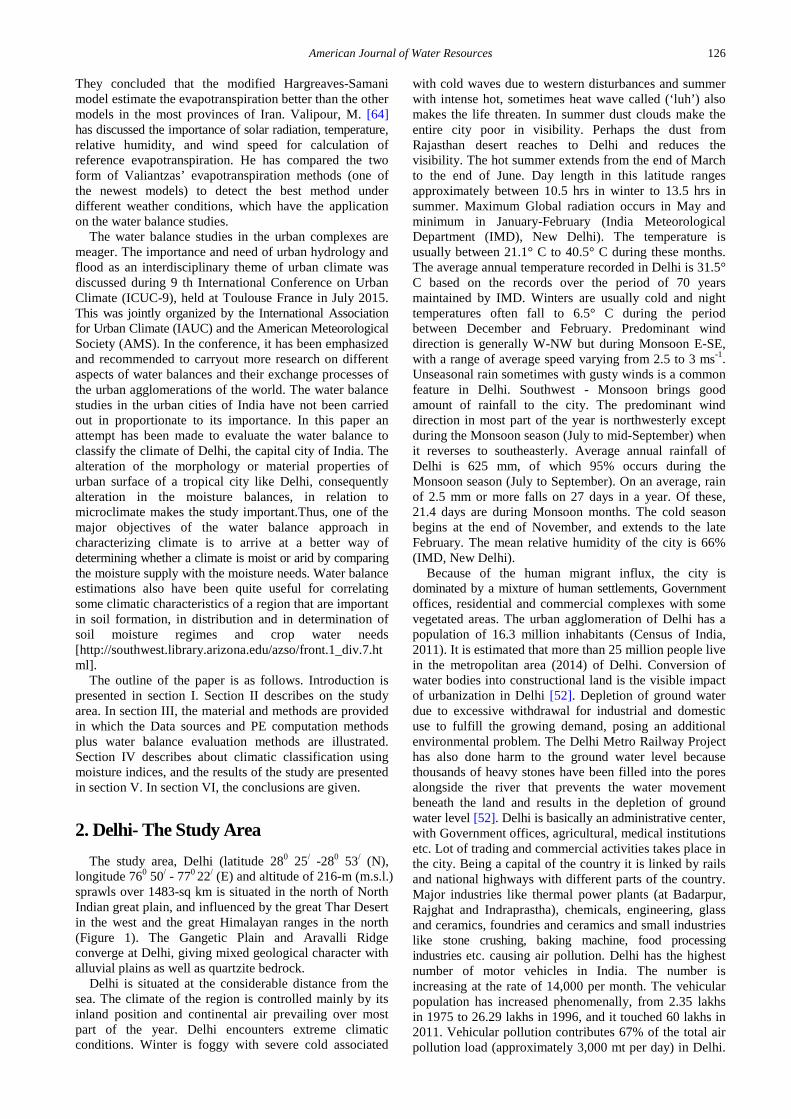
Figure 1. Map of a tropical city Delhi, the study area
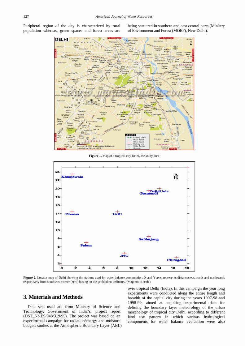
Figure 2. Locator map of Delhi showing the stations used for water balance computation. X and Y axes represents distances eastwards and northwards respectively from southwest corner (zero) basing on the gridded co-ordinates. (Map not to scale)
3. Materials and Methods Data sets used are from Ministry of Science and
Technology, Government of India’s, project report (DST_No.ES/048/319/95). The project was based on an experimental campaign for radiation/energy and moisture budgets studies at the Atmospheric Boundary Layer (ABL)
over tropical Delhi (India). In this campaign the year long experiments were conducted along the entire length and breadth of the capital city during the years 1997-98 and 1998-99, aimed at acquiring experimental data for defining the boundary layer meteorology of the urban morphology of tropical city Delhi, according to different land use pattern in which various hydrological components for water balance evaluation were also
American Journal of Water Resources 128
collected and procured from different Government nodal agencies. Details are described by Padmanabhamurty [48,49], Das [18] Das et al., [19]. The P and mean temperature (for the computation of PE) data are obtained from different Government nodal agencies, namely India Meteorological Department (IMD), Indian Agricultural Research Institute (IARI) and Jawaharlal Nehru University (JNU) / Centre for the Regional Studies (CSRD). Meteorological stations for which data were collected are Safdarjung Airport, Palam Airport, IARI, JNU, Delhi University (DU), ChiragDelhi, Gurmandi, Dhansa and Kanjhawala for the years 1997 and 1998. Locator map of all the meteorological stations are shown in Figure 2. The P data was available for all the meteorological stations as mentioned above. But the temperature data was only available for Safdarjung Airport, Palam Airport, IARI and JNU, therefore, temperature was spatially interpolated to fill the gap in the data sparse stations. Using these interpolated temperatures only PE was computed for those stations where temperature data was not available. Also, for the station Kanjhawala, the P data was available from June to December only for 1997, hence, P values at Safdarjung Airport as reported in Climatological Table (1951-80) published by IMD is utilized for filling the missing months data.
3.1. Water Balance Model Monthly water balance models have been used as a
means to examine the various components of the hydrologic cycle (e.g., P, evapotranspiration, and runoff), to estimate the global water balance [35,42]; and to develop climate classifications [59]. The water-balance model analyzes the allocation of water among various components of the hydrologic system using a accounting procedure based on the methodology originally presented by Thornthwaite [42,59]. Water balance model based on simple approach by Thornthwaite is widely used in different land use categories in wide and even small areas and regions.
The water balance model is expressed by the so-called ‘storage equation’ of the hydrologist as
P PE R S= + + ∆ Where, P = water supply to the region as precipitation in all its forms or from other sources, PE = total water loss by evaporation and transpiration, (Potential evapotranspiration) R = runoff from the area by subsurface or overload flow, and ∆S = change in the moisture status of the soil, (Soil moisture storage).
3.2. Methods of PE Evaluation for Water Balance Computation
Several methods have been described in literature for determining the PE [19,50]. Valipour, M. [66,70] has assessed the radiation-based, temperature based and MODIS data based models versus the FAO Penman–Monteith (FPM) model to determine the best model using linear regression under different weather conditions for PE and AE. Valipour, M. [67] has noted that Penman model estimates reference crop evapotranspiration better than other models in most provinces of Iran (15 provinces).
To compute the water balance at a place it is necessary to have i) Mean monthly/daily PE, ii) Mean monthly/daily P, and iii) Information on the water holding capacity of the depth of soil for which the balance is to be computed.
3.2.1. Thornthwaite's Formulae for PE According to the method of Thornthwaite the relation
between mean monthly temperature and PE (thermal efficiency) adjusted to a standard mean of 30 days each having 12 hours of possible sunshine is given by the equation:
101.6
aaT
PEI
=
Where, PE = Monthly potential evapotranspiration in Cms. Ta = Mean monthly air temperature (o C) a = Cubic function of I, given as,
( )
( )7 3 5 2
3
(6.75 10 ) 7.71 10
1.792 10 0.49
a I I
I
− −
−
= × × − × ×
+ × × +
I =Annual heat Index, given by
1.514 1.51412
1 5 5
.
na a
N
T TI i
mean heat index of the nth month
=
=
= ⋅ =
=
∑
This formulae gives unadjusted values of PE or thermal efficiency since the number of days in a month ranges from 28 to 31 (nearly 11%) and the number of hours of such as in the day between sunrise and sunset (when evapotranspiration principally takes place) varies with the latitude and seasons of the year, it becomes necessary to reduce or increase the unadjusted PE by a factor that varies with the latitude and the month under question.
3.2.2. Penman’s Formulae for PE The Penman’s formula describes evaporation (E) from
an open water surface, and was developed by Howard Penman in 1948. Penman's formulae requires daily mean temperature, wind speed, air pressure, and solar radiation to predict E. Simpler Hydrometeorological equations continue to be used where obtaining such data is impractical, to give comparable results within specific contexts, e.g. humid vs arid climates. Penman’s formula is widely used in computation of PE [19,50]. Valipour, M. [63] has applied the new mass transfer formulae for computation of evapotranspiration in Iran. He evidenced that the Penman model estimates the PE better than other models. The formula is,
( )
( )
( )
4
1
0.56 0.092 0.1 0.9
0.35 1100
1
A
d
a d
nR a bN
nT eN
ue eE
γ
γσ
γ
− + ∆ − + +
+ − +
=∆+
129 American Journal of Water Resources
Where, PE = Potential evapotranspiration in mm/day with surface reflection of 5% to open water, RA = Incident radiation outside the atmosphere on a horizontal surface expressed in mm of evaporable water per day, n = Duration of sunshine during the interval of estimate, N= Maximum duration of sunshine during the same time, σ = Stefan-Boltzmann constant, T= Temperature in degrees absolute, ed = Vapour pressure in mm of mercury, es = Saturation vapour pressure in mm of mercury, u = Daily wind run at 2 m above the ground in statute miles, γ = Psychometric constant, ∆ = rate of change with temperature of s.v.p.
These values are reduced by factor 0.7 as suggested by Penman to obtain PE.
The values of PE computed by Penman's method [18,50] for the representative station of Delhi has been compared with Thornthwaite’s method. On comparison with Thornthwaite's, it was found to be about 0.8% deviation from Penman’s method. The percentage departure of 1.68% from Penman was found for Delhi for Climatological normal data (IMD). Padmanabhamurty et al. [50] found the departure of about 2.34% in their water balance studies for some major cities of India.
3.3. Water Balance Evaluation Method
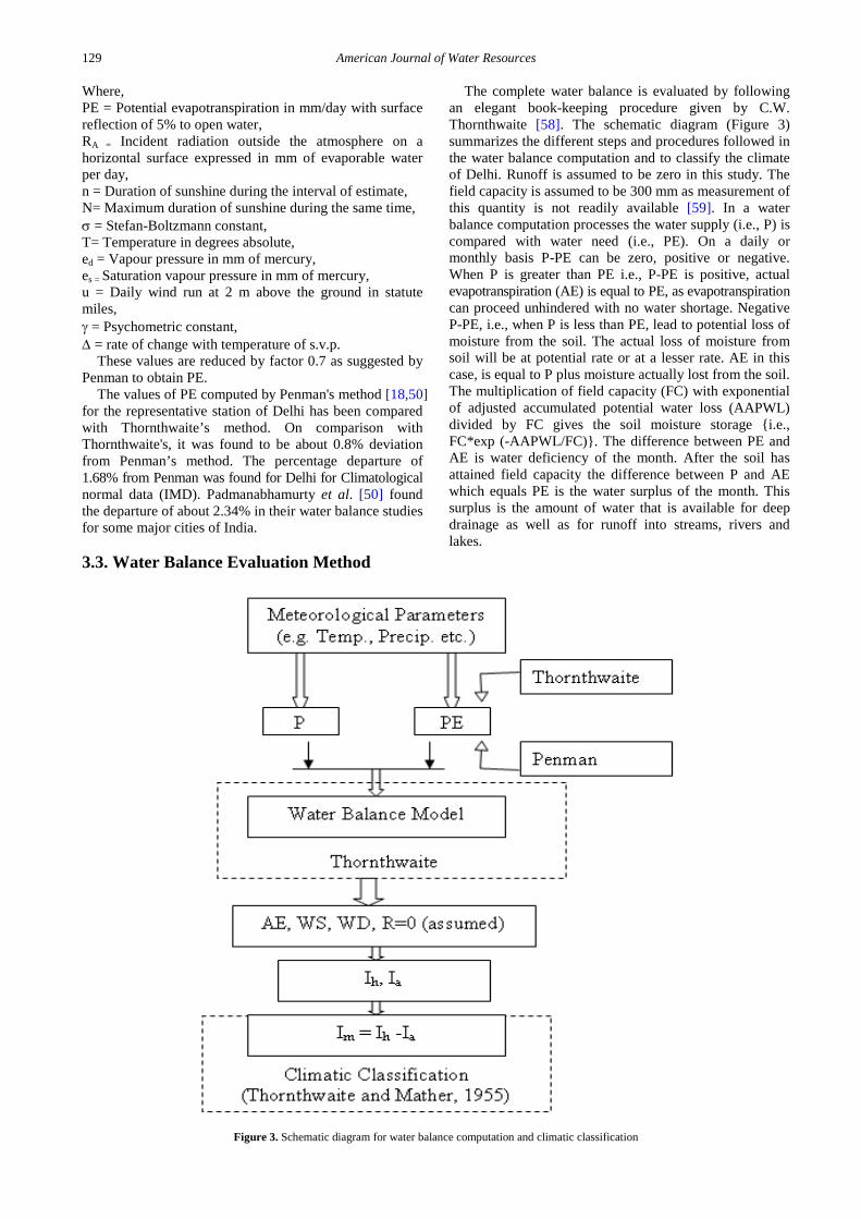
The complete water balance is evaluated by following an elegant book-keeping procedure given by C.W. Thornthwaite [58]. The schematic diagram (Figure 3) summarizes the different steps and procedures followed in the water balance computation and to classify the climate of Delhi. Runoff is assumed to be zero in this study. The field capacity is assumed to be 300 mm as measurement of this quantity is not readily available [59]. In a water balance computation processes the water supply (i.e., P) is compared with water need (i.e., PE). On a daily or monthly basis P-PE can be zero, positive or negative. When P is greater than PE i.e., P-PE is positive, actual evapotranspiration (AE) is equal to PE, as evapotranspiration can proceed unhindered with no water shortage. Negative P-PE, i.e., when P is less than PE, lead to potential loss of moisture from the soil. The actual loss of moisture from soil will be at potential rate or at a lesser rate. AE in this case, is equal to P plus moisture actually lost from the soil. The multiplication of field capacity (FC) with exponential of adjusted accumulated potential water loss (AAPWL) divided by FC gives the soil moisture storage {i.e., FC*exp (-AAPWL/FC)}. The difference between PE and AE is water deficiency of the month. After the soil has attained field capacity the difference between P and AE which equals PE is the water surplus of the month. This surplus is the amount of water that is available for deep drainage as well as for runoff into streams, rivers and lakes.
Figure 3. Schematic diagram for water balance computation and climatic classification

American Journal of Water Resources 130
4. Computation of Moisture Indices and Climatic Classification
Many scientists have studied the problem of how to express the daily or seasonal water balance of a site or region. The ability of scientists to describe water balance have been advanced significantly within the last few decades or so by the work of Penman [51] in England, Budyko [9] in the Soviet Union, Thornthwaite [59] in the United States and Grimmond et al. [25] in Canada. Each approach is quite different from the other and each has certain limitations. Thornthwaite's [59] procedure makes it possible to estimate soil moisture conditions of a site from the gains and losses of soil moisture over a certain interval of time, day, week or month. Thornthwaite and Mather [60] proposed a moisture index as part of a water balance model for a new classification system for climate. The formula developed by Thornthwaite [59], as modified by Thornthwaite and Mather [60], is used here, not necessarily because it is superior, but because it has been widely used worldwide by scientific community. The importance of this climatic classification has been recognized in many areas of knowledge and practice worldwide [34]. Although past climate research was focused on developing adequate methods for climate classification, current research is more concerned with understanding the patterns of climate change. However, the use of moisture indices as the indicator for climate change is still an incipient area of research [34].
The purpose of water balance studies is to investigate climate shift and to classify the region into climatic categories based on availability of WS and WD through water balance analysis. Moisture indices determine the moisture status and climatic type of a region. The moisture index (Im), humidity index (Ih) and aridity index (Ia) are computed as
12
1100h
i
WSIPE=
= ×
∑
12
1100a
i
WDIPE=
= ×
∑
and
( )m h aI I I= − [60]
Where, i = months The total annual WS is the summation of the entire
monthly WS’s during the year. Similarly, the annual WD and annual PE are obtained by summing the respective monthly values for the whole year from the book-keeping procedure for water balance.
The climate of Delhi is classified following the scheme of Thornthwaite and Mather [60] with the following limits of Im %.
Classification Type Limits of Im % Perhumid A 100 and above Humid B 20 to 100 Moist subhumid C2 0 to 20 Dry subhumid C1 -33.3 to 0 Semi-arid D -66.7 to -33.3
Arid E -100 to -66.7 The moisture indices may be positive or negative; the
positive values indicate moist/humid climates while the negative dry climates.
5. Results and Discussion The primary controls on the mean annual evapotranspiration
from a warm region are P and PE. Mean annual evapotranspiration cannot exceed the minimum of mean annual P and mean annual PE. Budyko [9,10] showed that the ratio of AE to P of a region is, in general, an increasing function of the aridity, or the dryness index, of the region. When P is equal to water need or potentialevaporation, the soil is at field capacity and no leaching takes place. When the soil water supply is greater than the need, there is a WS over time. When it is less, the soil moisture in the root zone is drawn upon by vegetation until the wilting point is reached and the moisture budget encounters WD. After the dry season, the soil-moisture reservoir must be replenished to field capacity before there can be a surplus again http://southwest.library.arizona.edu/azso/front.1_div.7.html). This study illustrates the small-scale spatial and temporal characteristics of water balance components over a tropical city Delhi to classify the climate of the city. The tables of water balance components for the different meteorological stations (Figure 2) are presented in the appendix I. However, the graphs illustrating the temporal variation of water balance components are shown only for five representative stations comprising Safdarjung and Palam Airports, JNU, DU and IARI, for rest of the stations the water balance component tables plus graphs are not shown for brevity and simplicity of the manuscript (can be produced upon request).
5.1. Temporal Variation of Water Balance Components
5.1.1. Station: Safdarjung Airport Temporal variations of water balance components at
Safdarjung Airport are shown in Figure 4a and Figure 4b. From the graphs it is evident that the variation of PE was almost symmetrical in both the years with maximum value (202 mm) during July and May (209.4 mm) in 1997 and 1998, respectively. The temporal variation patterns of P, AE and WD have showed erratic in nature. The values of P and AE both showed almost similar temporal variation pattern in 1997, but P was higher (maximum) in September month compared to AE in 1998. The values of P were lower in January, April and December. From the graphs it is clear that when P and AE were higher and lower, the WD was lower and higher, respectively. The WD value has shown the inverse variation pattern in relation to P and AE in both the years. On analyzing the monthly variation, it could be seen that WD showed lower values in January, August, November and December in 1997; again lower value of WD was noticed in January, February, August, September, November and December in 1998 also. The value of WD became less as the station gets recharged by monsoon rains. The March, April and May months show higher WD due to strong insolation and depletion of water from the surface cover of the locality. On an annual basis PE was higher by about 6.21% in 1998
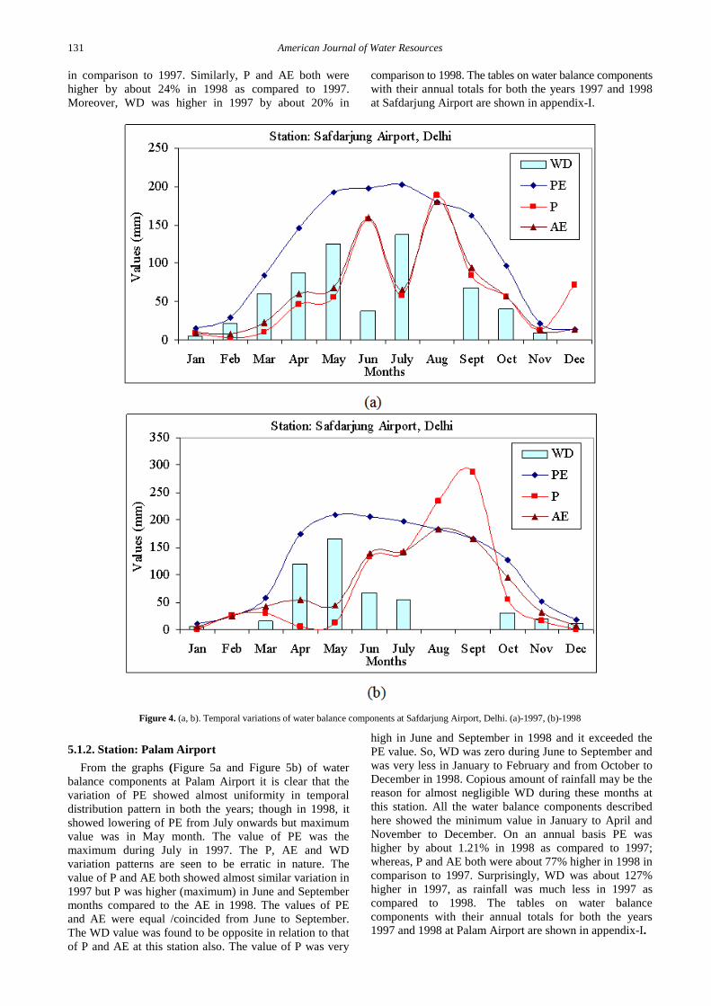
131 American Journal of Water Resources
in comparison to 1997. Similarly, P and AE both were higher by about 24% in 1998 as compared to 1997. Moreover, WD was higher in 1997 by about 20% in
comparison to 1998. The tables on water balance components with their annual totals for both the years 1997 and 1998 at Safdarjung Airport are shown in appendix-I.
Figure 4. (a, b). Temporal variations of water balance components at Safdarjung Airport, Delhi. (a)-1997, (b)-1998
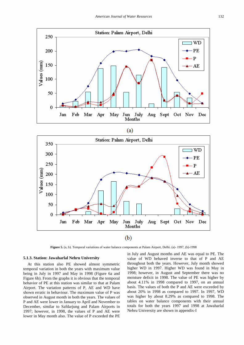
5.1.2. Station: Palam Airport From the graphs (Figure 5a and Figure 5b) of water
balance components at Palam Airport it is clear that the variation of PE showed almost uniformity in temporal distribution pattern in both the years; though in 1998, it showed lowering of PE from July onwards but maximum value was in May month. The value of PE was the maximum during July in 1997. The P, AE and WD variation patterns are seen to be erratic in nature. The value of P and AE both showed almost similar variation in 1997 but P was higher (maximum) in June and September months compared to the AE in 1998. The values of PE and AE were equal /coincided from June to September. The WD value was found to be opposite in relation to that of P and AE at this station also. The value of P was very
high in June and September in 1998 and it exceeded the PE value. So, WD was zero during June to September and was very less in January to February and from October to December in 1998. Copious amount of rainfall may be the reason for almost negligible WD during these months at this station. All the water balance components described here showed the minimum value in January to April and November to December. On an annual basis PE was higher by about 1.21% in 1998 as compared to 1997; whereas, P and AE both were about 77% higher in 1998 in comparison to 1997. Surprisingly, WD was about 127% higher in 1997, as rainfall was much less in 1997 as compared to 1998. The tables on water balance components with their annual totals for both the years 1997 and 1998 at Palam Airport are shown in appendix-I.
American Journal of Water Resources 132
Figure 5. (a, b). Temporal variations of water balance components at Palam Airport, Delhi. (a)- 1997, (b)-1998
5.1.3. Station: Jawaharlal Nehru University At this station also PE showed almost symmetric
temporal variation in both the years with maximum value being in July in 1997 and May in 1998 (Figure 6a and Figure 6b). From the graphs it is obvious that the temporal behavior of PE at this station was similar to that at Palam Airport. The variation patterns of P, AE and WD have shown erratic in behaviour. The maximum value of P was observed in August month in both the years. The values of P and AE were lower in January to April and November to December, similar to Safdarjung and Palam Airports in 1997; however, in 1998, the values of P and AE were lower in May month also. The value of P exceeded the PE
in July and August months and AE was equal to PE. The value of WD behaved inverse to that of P and AE throughout both the years. However, July month showed higher WD in 1997. Higher WD was found in May in 1998; however, in August and September there was no moisture deficit in 1998. The value of PE was higher by about 4.11% in 1998 compared to 1997, on an annual basis. The values of both the P and AE were exceeded by about 20% in 1998 as compared to 1997. In 1997, WD was higher by about 8.29% as compared to 1998. The tables on water balance components with their annual totals for both the years 1997 and 1998 at Jawaharlal Nehru University are shown in appendix-I

133 American Journal of Water Resources
Figure 6. (a, b). Temporal variations of water balance components at Jawaharlal Nehru University, Delhi. (a)- 1997, (b)-1998
5.1.4. Station: Delhi University The temporal variation pattern of PE depicted almost
uniform in nature in both the years with higher values during July and May in 1997 and 1998, respectively; and lower values in January-February and November- December (Figure 7a and Figure 7b). It is evident from the graphs that the variation patterns of P, AE and WD have followed the asymmetrical behavior in 1997 and 1998. The values of P and AE both have followed the similar variation patterns in both the years. The values of P and AE were higher (maximum) in August month in 1997; but during 1998, higher values were seen from July to September. During April and May months, the P and AE values were found to be lower in 1998. As expected at this
station also WD was higher on those months when P and AE were lower and vice-versa. During September in 1998, when P exceeded the PE; the value of WD was almost negligible or zero in August and September months, due to the replenish of surface strata by rainfall. February and March also showed zero WD in 1998. January-February and November-December are the months usually when water balance components were at their lower values. At this station the values of PE, P and AE were found to be higher by about 3%, 7.3% and 7.3%, respectively during 1998 as compared to 1997, on an annual basis. But, WD was higher in 1997 as compared to 1998 by about 3.5%. The tables on water balance components with their annual totals for both the years 1997 and 1998 at Delhi University are shown in appendix-I.

American Journal of Water Resources 134
Figure 7. (a, b). Temporal variations of water balance components at Delhi University, Delhi. (a)- 1997, (b)-1998
5.1.5. Station: Indian Agricultural Research Institute From the graph (Figure 8a and Figure 8b) the temporal
variation of PE is obvious. The maximum value of PE amounting to about 200 mm was observed in July in 1997; but in 1998, PE was maximum (about 208 mm) in May. The variation patterns of P, AE and WD have shown erratic in nature at this station also. The values of both the P and AE have shown similar temporal behavior in both the respective years. The P and AE have shown maximum values in August in 1997. In 1998, higher values of P and AE were seen in June with secondary maxima in August.
During August in 1997; when the P was maximum, there was less WD; however May month showed higher WD in 1998 indicating drier condition (lower P). There was less WD in June, August and September also in 1998, due to surface water recharge by rainfall. The values of PE, P and AE were found to be higher by about 3.01%, 21.46% and 21.46%, respectively during 1998 as compared to 1997, on an annual basis. The value of WD was higher by about 17.6% in 1997 on compared with 1998. The tables on water balance components with their annual totals for both the years 1997 and 1998 at Indian Agricultural Research Institute are shown in appendix-I.

135 American Journal of Water Resources
Figure 8. (a, b). Temporal variations of water balance components at Indian Agricultural Research Institute, Delhi. (a)- 1997, (b)-1998
5.2. Spatial Distribution of Water Balance Components
5.2.1. Precipitation (P) The spatial distribution of annual P over Delhi during
1997 and 1998 is obvious from isohyets (Figure 9a, and Figure 9b). Unseasonal rain due to western disturbances sometimes associated with thunder and gusty wind is a common feature in Delhi. Delhi gets a good amount of rainfall during South-West monsoon season. Distribution pattern of P over Delhi is uneven with high and low values in different localities. However, it is clear from the isohyets that during 1997 the urban areas with congested and densely built-up locations comprising Safdarjung Airport and DU showed areas of higher P than the
peripheral and rural areas like Khanjawala, Dhansa, Palam, JNU and ChiragDelhi. This may be due to augmentation of P by urban agglomeration that generate more condensation nuclei and thermal convection for cloud formation and hence P.
During 1998 the spatial distribution pattern was different than 1997. In 1998, the areas of higher P lay over Safdarjung and Palam Airport areas, whereas, the rural and peripheral regions viz. Khanjawala, Dhansa and JNU received lower rainfall.
The annual mean rainfall in different localities of Delhi in 1998 (795 mm) exceeded that in 1997 (612 mm) by about 30%. This could be perhaps in 1998; western disturbances rendered more P than previous year. The maximum annual P occurred at Safdarjung Airport (751 mm) in 1997 and at Palam Airport in 1998 (1057 mm).

American Journal of Water Resources 136
Minimum P was at Khanjawala in both the years amounting to 469 mm and 627 mm respectively. Percentage departure of P from mean of 1997 was maximum at Palam Airport and minimum at DU. During
1997 and 1998, Khanjawala received least P, whereas, Safdarjung Airport the highest in 1997 and Palam airport in 1998. It was found that P was more in the urban and suburban stations than their rural counterparts.
Figure 9. (a, b). Spatial distribution of Precipitation (P) mm over Delhi. (a)- Year 1997, (b) - Year 1998. X and Y axes represents distances eastwards and northwards respectively from southwest corner (zero) basing on the gridded co-ordinates
5.2.2. Potential Evapotranspiration (PE) The spatial distribution patterns of PE are shown in
(Figure 10a and Figure 10b). Thermal factor is the main
determinant of PE. The PE is the maximum amount of evaporation from the soil surfaces and transpiration from the plant cover when there is no dearth of moisture for full use.

137 American Journal of Water Resources
The spatial distribution patterns of PE over Delhi (Figure 10a and Figure 10b) are similar in 1997 and 1998 but differ in quantity. Spatial variation of PE indicates that higher values occurred in southern parts compared to northwest. The annual mean PE of all the stations in 1997 (1316 mm) exceeded that in 1998 (1369 mm) by 4%. Maximum PE in 1998 was 1457 mm at JNU and minimum at IARI amounting to 1299 mm. In 1997 also it was maximum at JNU (1400 mm) and minimum at IARI (1261 mm). Percentage departure of PE from the mean of
1997 was maximum at Safdarjung Airport, and minimum at Palam Airport. In both the years it is found that PE was more in the rural locations compared to their urban/semi-urban counterparts. This could be perhaps due to the less availability of surfaces from which evaporation takes places, that is, reduction of the evaporating surfaces in the urban areas due to their concrete, rocky, built-up and paved natured surfaces with scanty of vegetation, which reduces the PE.
Figure 10. (a, b). Spatial distribution of PE (mm) over Delhi. (a)- Year 1997, (b) - Year 1998. X and Y axes represents distances eastwards and northwards respectively from southwest corner (zero) basing on the gridded co-ordinates
5.2.3. Actual Evapotranspiration (AE) The Spatial distribution of AE is shown in Figure11a
and Figure 11b. Besides P, thermal conditions also affect
the AE. The AE is the quantity of water that is actually removed from a surface due to the processes of evaporation and transpiration.
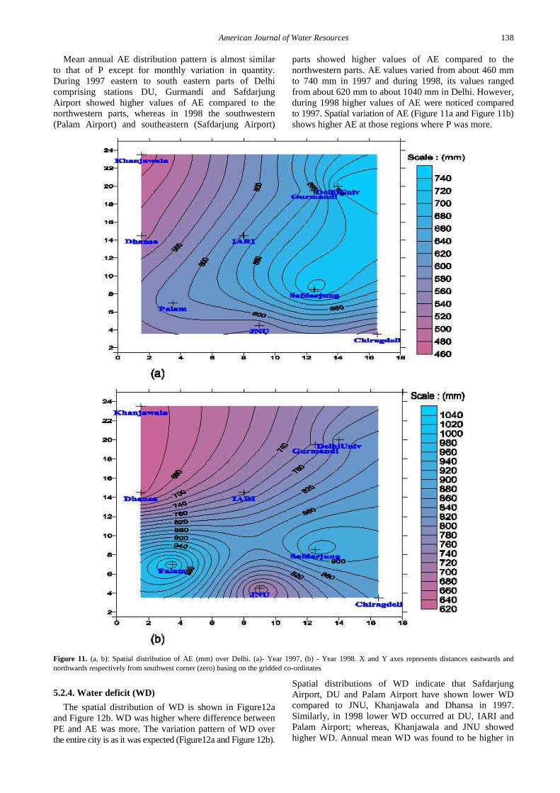
American Journal of Water Resources 138
Mean annual AE distribution pattern is almost similar to that of P except for monthly variation in quantity. During 1997 eastern to south eastern parts of Delhi comprising stations DU, Gurmandi and Safdarjung Airport showed higher values of AE compared to the northwestern parts, whereas in 1998 the southwestern (Palam Airport) and southeastern (Safdarjung Airport)
parts showed higher values of AE compared to the northwestern parts. AE values varied from about 460 mm to 740 mm in 1997 and during 1998, its values ranged from about 620 mm to about 1040 mm in Delhi. However, during 1998 higher values of AE were noticed compared to 1997. Spatial variation of AE (Figure 11a and Figure 11b) shows higher AE at those regions where P was more.
Figure 11. (a, b): Spatial distribution of AE (mm) over Delhi. (a)- Year 1997, (b) - Year 1998. X and Y axes represents distances eastwards and northwards respectively from southwest corner (zero) basing on the gridded co-ordinates
5.2.4. Water deficit (WD) The spatial distribution of WD is shown in Figure12a
and Figure 12b. WD was higher where difference between PE and AE was more. The variation pattern of WD over the entire city is as it was expected (Figure12a and Figure 12b).
Spatial distributions of WD indicate that Safdarjung Airport, DU and Palam Airport have shown lower WD compared to JNU, Khanjawala and Dhansa in 1997. Similarly, in 1998 lower WD occurred at DU, IARI and Palam Airport; whereas, Khanjawala and JNU showed higher WD. Annual mean WD was found to be higher in

139 American Journal of Water Resources
1997 than in 1998 by 23%. The maximum WD of 750 mm was at JNU and minimum of 346 mm was noticed at Palam Airport in 1998. Corresponding values in 1997 were 813 mm at JNU and 504 mm at DU. Higher values of WD were also found in rural locations than at the urban
and semi–urban locations. This may be due to uneven rainfall distribution combined with open wastewater drains spread over the entire urban and semi–urban areas, which outweigh the rural moisture conditions. There was no WS at any station either in 1997 or 1998.
Figure 12 (a, b): Spatial distribution of WD (mm) over Delhi. (a)- Year 1997, (b) - Year 1998. X and Y axes represents distances eastwards and northwards respectively from southwest corner (zero) basing on the gridded co-ordinates
5.3. Moisture Indices and Climatic Classification of Delhi
Water balance study in relation to climate is one of the important disciplines of applied climatology. Temperature and P alone are poor descriptors of climate. The amount of P does not indicate whether a climate is moist or dry
unless the water need of the site can be compared with it. And temperature does not really reveal the energy that is available for plant growth and development unless the moisture condition of the soil is known (http://southwest.library.arizona.edu/azso/front.1_div.7.html).
The purpose of moisture balance studies is to classify the region into climatic categories based on availability of

American Journal of Water Resources 140
WS and WD. Climatic classification requires computation of Ia, Ih and finally Im. Ia is the percentage ratio of the total annual WD to the total annual water need or PE. Similarly, Ih is the percentage ratio of the total annual WS to the total annual water need or PE, and finally Im is obtained by subtracting Ia from the Ih, that is, Im = (Ih - Ia ).
All the required indices have been calculated for all the locations comprising diverse land-use pattern for the year 1997 and 1998. Ih was found to be zero for all the stations as there was no water surplus. The spatial distribution pattern of Ia (Figure 13a and Figure 13b) indicates that northeastern parts of the city shown lower Ia values;
whereas, the entire southern and northwestern regions showed higher values in 1997. But in 1998 the spatial distribution pattern of Ia was quite different than 1997. The southwestern part showed lower aridity indices than other parts of the city. It was found that Ia was higher in 1997 than 1998 by 26%. The maximum value of Ia was 62% at Khanjawala and minimum was 39% at DU in 1997. Again it was maximum (51.7%) at Khanjawala and minimum (24%) at Palam Airport in 1998. On the whole in tropical mega city Delhi, Ia was found to be higher in 1997 as compared to 1998.
Figure 13. (a, b). Spatial distribution of Ia (%) over Delhi. (a)- Year 1997, (b)- Year 1998. X and Y axes represents distances eastwards and northwards respectively from southwest corner (zero) basing on the gridded co-ordinates
It is clear that, Im have been computed for all the stations as indicated in locator map for both the years
1997 and 1998. From the spatial distribution patterns of Im (Figure 14a and Figure 14b) for the year 1997, it is
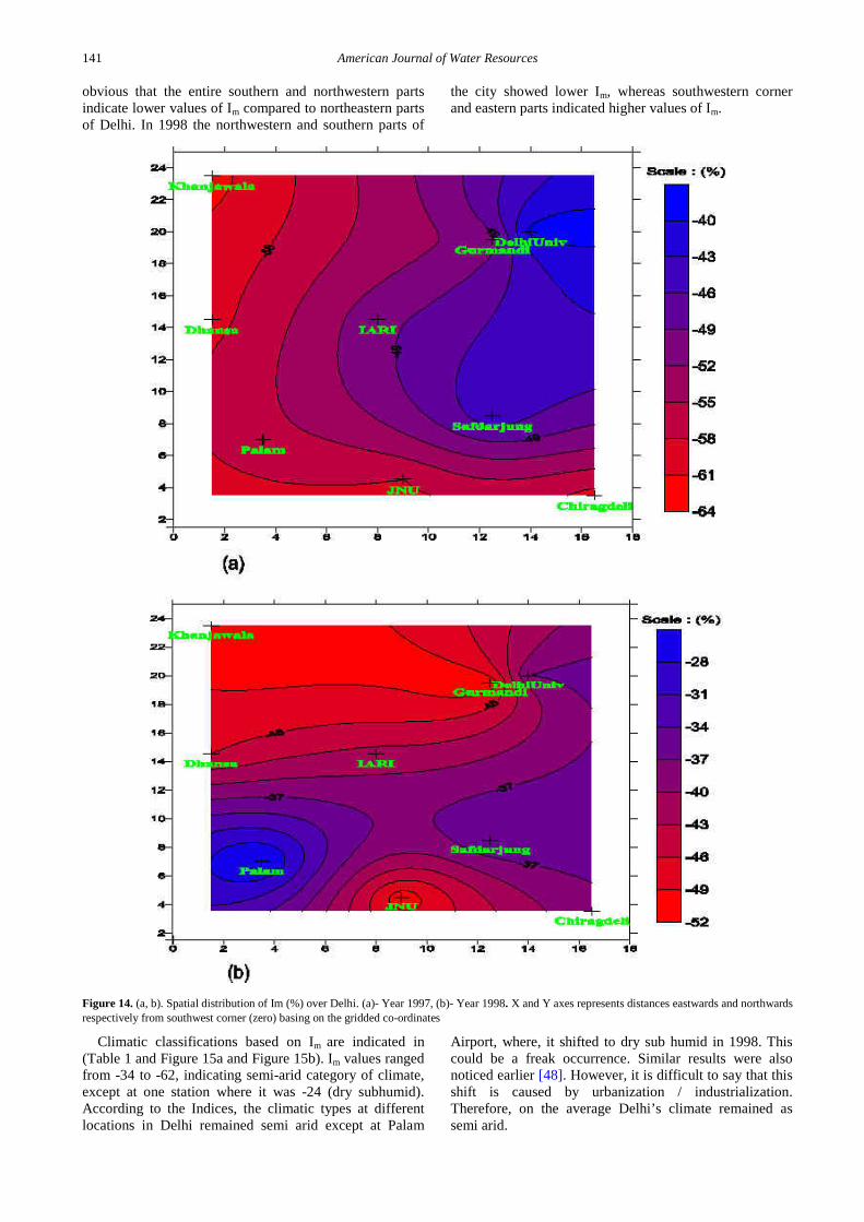
141 American Journal of Water Resources
obvious that the entire southern and northwestern parts indicate lower values of Im compared to northeastern parts of Delhi. In 1998 the northwestern and southern parts of
the city showed lower Im, whereas southwestern corner and eastern parts indicated higher values of Im.
Figure 14. (a, b). Spatial distribution of Im (%) over Delhi. (a)- Year 1997, (b)- Year 1998. X and Y axes represents distances eastwards and northwards respectively from southwest corner (zero) basing on the gridded co-ordinates
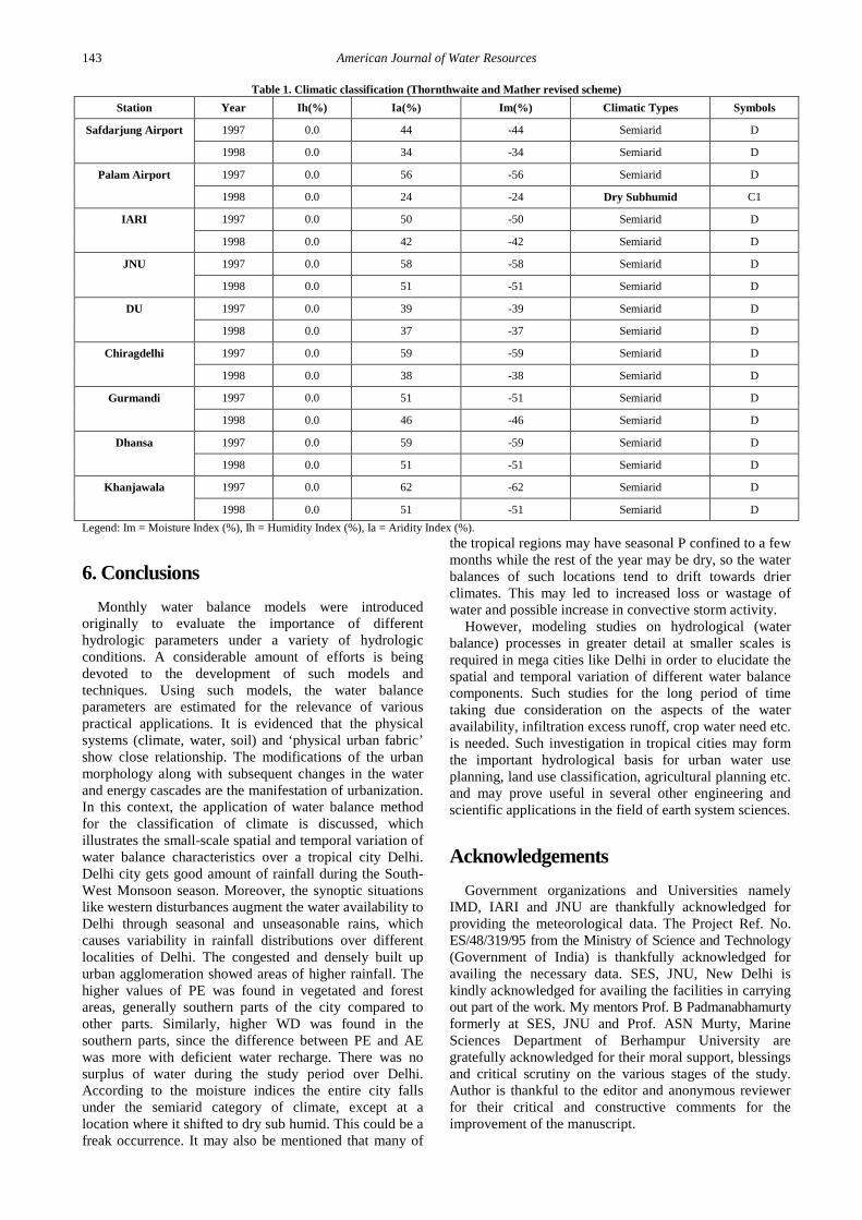
Climatic classifications based on Im are indicated in (Table 1 and Figure 15a and Figure 15b). Im values ranged from -34 to -62, indicating semi-arid category of climate, except at one station where it was -24 (dry subhumid). According to the Indices, the climatic types at different locations in Delhi remained semi arid except at Palam
Airport, where, it shifted to dry sub humid in 1998. This could be a freak occurrence. Similar results were also noticed earlier [48]. However, it is difficult to say that this shift is caused by urbanization / industrialization. Therefore, on the average Delhi’s climate remained as semi arid.

American Journal of Water Resources 142
Figure 15. (a, b). Climatic types at different stations over Delhi. (a)-Year 1997, (b) - Year 1998. X and Y axes represents distances eastwards and northwards respectively from southwest corner (zero) basing on the gridded co-ordinates
143 American Journal of Water Resources
Table 1. Climatic classification (Thornthwaite and Mather revised scheme) Station Year Ih(%) Ia(%) Im(%) Climatic Types Symbols
Safdarjung Airport 1997 0.0 44 -44 Semiarid D
1998 0.0 34 -34 Semiarid D
Palam Airport 1997 0.0 56 -56 Semiarid D
1998 0.0 24 -24 Dry Subhumid C1
IARI 1997 0.0 50 -50 Semiarid D
1998 0.0 42 -42 Semiarid D
JNU 1997 0.0 58 -58 Semiarid D
1998 0.0 51 -51 Semiarid D
DU 1997 0.0 39 -39 Semiarid D
1998 0.0 37 -37 Semiarid D
Chiragdelhi 1997 0.0 59 -59 Semiarid D
1998 0.0 38 -38 Semiarid D
Gurmandi 1997 0.0 51 -51 Semiarid D
1998 0.0 46 -46 Semiarid D
Dhansa 1997 0.0 59 -59 Semiarid D
1998 0.0 51 -51 Semiarid D
Khanjawala 1997 0.0 62 -62 Semiarid D
1998 0.0 51 -51 Semiarid D Legend: Im = Moisture Index (%), Ih = Humidity Index (%), Ia = Aridity Index (%).
6. Conclusions Monthly water balance models were introduced
originally to evaluate the importance of different hydrologic parameters under a variety of hydrologic conditions. A considerable amount of efforts is being devoted to the development of such models and techniques. Using such models, the water balance parameters are estimated for the relevance of various practical applications. It is evidenced that the physical systems (climate, water, soil) and ‘physical urban fabric’ show close relationship. The modifications of the urban morphology along with subsequent changes in the water and energy cascades are the manifestation of urbanization. In this context, the application of water balance method for the classification of climate is discussed, which illustrates the small-scale spatial and temporal variation of water balance characteristics over a tropical city Delhi. Delhi city gets good amount of rainfall during the South-West Monsoon season. Moreover, the synoptic situations like western disturbances augment the water availability to Delhi through seasonal and unseasonable rains, which causes variability in rainfall distributions over different localities of Delhi. The congested and densely built up urban agglomeration showed areas of higher rainfall. The higher values of PE was found in vegetated and forest areas, generally southern parts of the city compared to other parts. Similarly, higher WD was found in the southern parts, since the difference between PE and AE was more with deficient water recharge. There was no surplus of water during the study period over Delhi. According to the moisture indices the entire city falls under the semiarid category of climate, except at a location where it shifted to dry sub humid. This could be a freak occurrence. It may also be mentioned that many of
the tropical regions may have seasonal P confined to a few months while the rest of the year may be dry, so the water balances of such locations tend to drift towards drier climates. This may led to increased loss or wastage of water and possible increase in convective storm activity.
However, modeling studies on hydrological (water balance) processes in greater detail at smaller scales is required in mega cities like Delhi in order to elucidate the spatial and temporal variation of different water balance components. Such studies for the long period of time taking due consideration on the aspects of the water availability, infiltration excess runoff, crop water need etc. is needed. Such investigation in tropical cities may form the important hydrological basis for urban water use planning, land use classification, agricultural planning etc. and may prove useful in several other engineering and scientific applications in the field of earth system sciences.
Acknowledgements Government organizations and Universities namely
IMD, IARI and JNU are thankfully acknowledged for providing the meteorological data. The Project Ref. No. ES/48/319/95 from the Ministry of Science and Technology (Government of India) is thankfully acknowledged for availing the necessary data. SES, JNU, New Delhi is kindly acknowledged for availing the facilities in carrying out part of the work. My mentors Prof. B Padmanabhamurty formerly at SES, JNU and Prof. ASN Murty, Marine Sciences Department of Berhampur University are gratefully acknowledged for their moral support, blessings and critical scrutiny on the various stages of the study. Author is thankful to the editor and anonymous reviewer for their critical and constructive comments for the improvement of the manuscript.

American Journal of Water Resources 144
References [1] Andrieu, H., Chocat, B. (2004): Introduction to the special issue
on urban hydrology. Journal of Hydrology, 299 (3–4), 163-165. [2] Ashby, W.C., Fritts, H.C. (1972): Tree growth, air pollution, and
Climate near La Porte, Ind. Bull. Amer. Metreol., Soc., 53, 246-251.
[3] Aston, A. (1977): Water resources and consumption in Hong Kong. Urban Ecol., 2, 327-353.
[4] Atkinson, S. E., Woods, R. A., Sivapalan, M. (2002), Climate and landscape controls on water balance model complexity over changing timescales. Water Resour. Res., 38(12), 1314.
[5] Baik, J.-J., Kim, J.-J. (1999): A numerical study of flow and pollutant dispersion characteristics in urban street canyons. Journal of Applied Meteorology, 38, 1576-1589.
[6] Beebe, R.C.,. Morgan, Jr., G. M (1972): Synoptic analysis of summer rainfall periods exhibiting urban effects. Preprints conf. On urban environ. and second conf. Biometeorol. Amer. Meteorol. Soc., 173-176.
[7] Bell, F.C. (1972): The acquisition, consumption and elimination of water by Sydney urban system. Proc. Ecol. Soc. Aust., 7,160-176.
[8] Bhaskar, A. S., Welty, C. (2012): Water Balances along an Urban-to-Rural Gradient of Metropolitan Baltimore, 2001-2009. Environmental & Engineering Geoscience, Vol. XVIII, No. 1, 37-50.
[9] Budyko, M. I. (1974): Climate and Life, Elsevier, New York. [10] Budyko, M.I. (1982): The Earth’s Climate: Past and future.
Academic Press Inc. London, 307 pp. [11] Campbell, T. (1982): La ciudad de Mexico como ecosistema.
Ciencias Urbanas, 1, 28-35. [12] Changnon, S.A. Jr. (1968): The Laporte anomaly – fact or fiction?
Bull Amer. Meteorol. Soc., 49, 4-11. [13] Changnon, S.A. Jr., Huff, F.A., Semolina, R.G. (1971):
METROMEX: an investigation on inadvertent weather modification. Bull. Amer. Meteorol. Soc., 52, 958-967.
[14] Changnon, S.A. Jr., Semolina, R.G., Lowery, W.P.(1972): Inadvertent modifications of urban environments. Preprints conf. urban environs. and second conf. Biometeorol., Amer. Meteorol. Soc., 165-172.
[15] Changnon, S.A.Jr. (1970): Reply, Bull. Amer. Meteorol. Soc., 51, 337-343.
[16] Changnon, S.A.Jr. (1971): Comments on the effect on rainfall of a large steel works. J. Appl. Metreol., 10, 165-168.
[17] Changnon, S.A.Jr. (1972): Urban effect on thunderstorm and hailstorm frequencies. Conf. on urban environ. and second conf. on Biometeorol., Amer. Meteorol. Soc., 177-184.
[18] Das, Y. (2002): Spatial and temporal distribution of radiation/energy/moisture budgets over Delhi, Ph.D. Thesis, Berhampur University, Berhampur, India, 125.
[19] Das, Y., Padmanabhamurty, B., Murty, A.S.N. (2009): Energy and water balance studies in the boundary layer over Delhi (India). Contributions to Geophysics and Geodesy, 39 (2), 163-185.
[20] Eagleman, J. R. (1967): Pan evaporation, potential and actual evaporation. Journal of Applied Meteorology, 6 (3), 482-488.
[21] Farmer, D., Sivapalan, M., Jothityangkoon, C. (2003): Climate, soil, and vegetation controls upon the variability of water balance in temperate and semiarid landscapes: Downward approach to water balance analysis. Water Resour. Res., 39(2), 1035.
[22] Givoni, B. (1969): Man, Climate and Architecture. Elsevier Pub.Co. Ltd. 364.
[23] Grimmond, C.S.B., Oke, T. R., Styen, D.G. (1986): Urban water balance I: A model for daily totals. Water Resources Research, 22, 1397-1403.
[24] Grimmond, C.S.B., Oke, T.R (2002): Turbulent heat fluxes in urban areas: observations and a Local-scale Urban Meteorological Parameterization Scheme (LUMPS). Journal of Applied Meteorology, 41, 792-810.
[25] Grimmond, C.S.B., Oke, T.R. (1986): Urban water balance-II: Results from a suburb of Vancouver, British Columbia. Water resource research, 22, 10, 1404-1412.
[26] Grimmond, C.S.B., Oke, T.R. (1999): Evapotranspiration rates in urban areas. Impacts of Urban growth on surface water and groundwater quality (Proceedings of IUGG '99 Symposium HS5, Birmingham, July 1999). IAHS Publ, no. 259.
[27] Hidore, J.F. (1971): The effects of accidental weather on the flow of the Kankakee River. Bull Amer. Meteorol. Soc., 52, 99-103.
[28] Holzman, B.G. (1971b): More on the La Porte fallacy (with reply by Hidore). Bull. Amer. Meteorol. Soc., 52, 572-574.
[29] Holzman, B.G., Thom, H.C.S. (1970): The La Porte precipitation anomaly. Bull. Amer. Metreol. Soc., 51, 335-337.
[30] Huff, F.A., Changnon Jr. S.A. (1972a): Inadvertent precipitation modification by major urban area. Proc. Third conf. Weath. Modf., Amer. Meteorol. Soc., 73-78.
[31] Kyuma, K. (1971): 'Climate of South and Southeast Asia According to Thornthwaite's Classification Scheme. Southeast Asian Studies (Kyoto), .9 (1): 1 36 1 58.
[32] Kyuma, K. (1972): Numerical Classification of the Climate of South and Southeast Asia. Southeast Asian Studies (Kyoto), 9 (4): 502-521.
[33] Landsberg, H.E. (1972): Inadvertent atmospheric modifications through urbanization. Tech. Note No. BN 741, Instit. Fluid Dyn. Appl. Math., Univ. Maryland, 73.
[34] Leao, S. (2014): Mapping 100 Years of Thornthwaite Moisture Index: Impact of Climate Change in Victoria, Australia. Geographical Research, 52 (3), 309-327.
[35] Legates, D.R., McCabe, G.J. (2005): A re-evaluation of the average annual global water balance: Physical Geography, v. 26, 467-479.
[36] Leopold, L. B. (1968): Hydrology for Urban Land Planning—A Guidebook on the Hydrologic Effects of Urban Land Use: U.S. Geological Survey, Circular, 554, 18.
[37] Lindh, G. (1978): Urban hydrological modeling and catchment research in Swede. [In Research on Urban Hydrology], Edited by B. McPherson, 2 229-265. UNESCO, Paris.
[38] Lull, H.W., Sopper, W.E. (1969): Hydrologic effects from urbanization of forested watersheds in the Northeast, USDA, Forest Service Research Paper, NE-146, 31.
[39] L'vovich, M.I., Chernogayeva, G.M. (1977): Transformation of the water balance within the city of Moscow. Sov. Geogr., 18, 302-312.
[40] Maruyama, E. (1978): Fluctuation of Paddy Yield and Water Resources in Southeast Asia. In: Climatic Change and Food Production (Eds.K. Takahashi and M. M. Yoshin), 155-166. Tokyo: University of Tokyo Press.
[41] Mather, J.R. (1974): Climatology: Fundamental and Application. McGraw-Hill Book Company. USA.
[42] McCabe, G.J., Markstrom, S.L. (2007): A monthly water-balance model driven by a graphical user interface: U.S. Geological Survey Open-File report -1088, 6.
[43] Moore, W.L. Morgan, C.W (1969): Effects of watershed changes on Stream flow, Univ. of Texas Press, Austin.
[44] Muller, R.D. (1968): Some effects of urbanization on runoff as evaluated by Thornthwaite water balance models. Proc. 3rd. Ann. Conf. Amer. Water Resources Asso. 245.
[45] Novotny, V. (1995): Non-point pollution and Urban Stormwater Management. Technomic Publishing Co., Lancaster, PA.
[46] Ogden, T.L. (1969): The effect of rainfall on a large steel works. J. Appl. Meteorol, 8, 585-591.
[47] Padmanabhamurty, B. (1981): Inadvertent modification of water balance- A problem of urban hydrology. Vayu Mandal, 36-39.
[48] Padmanabhamurty, B. (1994): 'Urban-rural energy and moisture balance studies': Final Report on DST Project. Ref. No. ES/63/018/86., (Govt. of India).
[49] Padmanabhamurty, B. (1999): ' Spatial and temporal variations of radiation, energy and moisture budgets in the boundary layer at Delhi': Final Report on DST Project. Ref. No. ES/48/319/95, (Govt. of India).
[50] Padmanabhamurty, B., Satyanarayana, C.V.V. Rao., Dakshinamurti, J. (1970): On the water balances of some Indian stations. Journal of Hydrology, 11, 169-184.
[51] Penman, H.L. (1948): Natural evaporation from open waters, bare soil and grass. Proc. Roy. Soc. London, A 193, 120.
[52] Pushpam, (2004): Ecosystem Services of Floodplains: An Exploration of Water Recharge Potential of the Yamuna Floodplain for Delhi. Paper Presented at the conference on Market Development of Water & Waste Technologies through Environmental Economics, 28th-29th May 2004, Paris.
[53] Rahimi, S., Sefidkouhi, M.A.G, Raeini-Sarjaz, M. Valipour, M. (2015f): Estimation of actual evapotranspiration by using MODIS images (a case study: Tajan catchment. Archives of Agronomy and Soil Science, 61(5), 695-709.
[54] Rao, K.N., George, C. J., Ramasastri, K.S. (1976): The climatic water balance of India. Vol. XXXII, Part II, (IMD, Publication).

145 American Journal of Water Resources
[55] Sankarasubramanian, A., Vogel, R.M.(2002): Annual hydroclimatology of the United States. Water Resour. Res., 38(6), 1083.
[56] Schaakel, J.C. Jr. (1972): Water and the city; in urbanization and Environment, Detwyler, T.R. and M.G. Marcus (eds.), Duxbury Press, 97-134.
[57] Shepherd, J. M. (2005): A review of current investigations of urban-induced rainfall and recommendations for the future: Earth Interactions, 9, 1-27.
[58] Subrahmanyam, V.P. (1982): Water balance and its application. (With special reference to India). Monograph, Andhra University Press, Waltair, Visakhapatnam, India, 102.
[59] Thornthwaite, C.W. (1948): An Approach toward a Rational Classification of Climate. Geog. Rev., 38: 55-94.
[60] Thornthwaite, C.W. Mather, J.R (1955): Water balance publication in climatology. Drexel Ins. of Tech., 8(1).
[61] Trauth, R., Xanthopoulos, C. (1997): Non-point pollution of groundwater in urban areas. Water Research, 31, 2711-2718.
[62] Valipour, M. (2014a): Analysis of potential evapotranspiration using limited weather data. Appl. Water Sci..
[63] Valipour, M. (2014b): Application of new mass transfer formulae for computation of evapotranspiration. Journal of Applied Water Engineering and Research,2(1), 33-46.
[64] Valipour, M. (2014c): Importance of solar radiation, temperature, relative humidity, and wind speed for calculation of reference evapotranspiration. Archives of Agronomy and Soil Science, 61(2).
[65] Valipour, M. (2014d): Investigation of Valiantzas’ evapotranspiration equation in Iran. Theoretical and Applied Climatology, 121(1-2), 267-278.
[66] Valipour, M. (2015a): Study of different climatic conditions to assess the role of solar radiation in reference crop evapotranspiration equations. Archives of Agronomy and Soil Science, 61(5), 679-694.
[67] Valipour, M. (2015b): Calibration of mass transfer-based models to predict reference crop evapotranspiration. Appl Water Sci.
[68] Valipour, M. (2015c): Comparative Evaluation of Radiation-Based Methods for Estimation of Potential Evapotranspiration. Journal of Hydrologic Engineering, 20(5):04014068.
[69] Valipour, M. (2015d): Evaluation of radiation methods to study potential evapotranspiration of 31 provinces. Meteorology and Atmospheric Physics, 127(3), 289-303.
[70] Valipour, M. (2015e): Temperature analysis of reference evapotranspiration models. Meteorological Applications, 22(3), 385-394.
[71] Valipour, M. Eslamian, S. (2014e): Analysis of potential evapotranspiration using 11 modified temperature-based models. Int. J. of Hydrology Science and Technology, 4(3)192-207.
[72] Watkins (1963): Research on surface –water drainage. Proc. Instit. Civil Engin., 24, 305-330.
[73] Wolock, D. M., McCabe, G. J. (1999): Explaining spatial variability in mean annual runoff in the conterminous United States. Clim. Res., 11, 149-159.
[74] Woods, R. (2003): The relative roles of climate, soil, vegetation and topography in determining seasonal and long-term catchment dynamics. Adv. Water Resour., 26, 295-309.
Appendix –I 1. Water Balance computation table at Safdarjung Airport (28.5844° N, 77.2058° E), Delhi.
Height (amsl)=216 m. Field capacity=300 mm (assumed). Year: 1997
Item Jan Feb Mar Apr May Jun July Aug Sept Oct Nov Dec Annual PE 15.0 28.5 83.8 146.0 192.3 197.2 202.0 180.2 162.1 96.9 21.0 13.2 1338.2 P 9.0 2.3 10.4 46.6 55.2 157.0 57.8 187.9 84.3 56.0 12.6 71.8 750.9
AE 10.3 7.7 23.2 59.7 67.4 159.6 64.8 180.2 94.6 57.1 12.8 13.2 750.7 WD 4.7 20.8 60.6 86.3 124.9 37.6 137.2 0.0 67.5 39.8 8.2 0.0 587.5 WS 0.0 0.0 0.0 0.0 0.0 0.0 0.0 0.0 0.0 0.0 0.0 0.0 0.0
Year:1998 Item Jan Feb Mar Apr May Jun July Aug Sept Oct Nov Dec Annual PE 10.5 24.9 57.6 174.1 209.4 205.6 197.1 183.1 164.5 125.8 51.1 17.7 1421.4 P 0.0 26.0 30.0 5.0 13.1 131.2 138.1 234.2 286.7 54.7 15.0 0.0 934.0
AE 4.4 24.9 42.0 53.7 44.0 138.5 142.8 183.1 164.5 95.8 32.4 7.8 934.0 WD 6.1 0.0 15.6 120.4 165.4 67.1 54.3 0.0 0.0 30.0 18.7 9.9 487.4 WS 0.0 0.0 0.0 0.0 0.0 0.0 0.0 0.0 0.0 0.0 0.0 0.0 0.0
2. Water Balance computation table at Palam Airport (8.5686° N, 77.1122° E), Delhi. Height (amsl)=216 m. Field capacity=300 mm (assumed).
Year: 1997 Item Jan Feb Mar Apr May Jun July Aug Sept Oct Nov Dec Annual PE 14.0 27.3 75.7 157.0 198.6 199.8 204.3 182.3 167.8 96.5 48.5 14.9 1386.7 P 6.3 1.2 14.2 8.5 43.8 144.3 85.8 168.5 23.9 41.8 14.4 48.5 601.2
AE 7.2 4.1 20.1 18.7 50.2 145.9 88.4 168.7 25.8 42.3 14.7 14.9 601.2 WD 6.8 23.2 55.6 138.3 148.4 53.9 115.9 13.6 142.0 54.2 33.8 0.0 785.6 WS 0.0 0.0 0.0 0.0 0.0 0.0 0.0 0.0 0.0 0.0 0.0 0.0 0.0
Year: 1998 Item Jan Feb Mar Apr May Jun July Aug Sept Oct Nov Dec Annual PE 11.3 25.8 62 174.1 213.2 206.5 198.2 176.4 165.2 92.9 57.8 20.2 1403.6 P 1 23 16.7 4.4 6.1 279.1 226.1 186.6 260.1 45 9.5 0 1057.6
AE 6.6 24.5 38.9 63.4 44.7 206.5 198.2 176.4 165.2 81.1 40.5 11.5 1057.5 WD 4.7 1.3 23.1 110.7 168.5 0 0 0 0 11.8 17.3 8.7 346.1 WS 0 0 0 0 0 0 0 0 0 0 0 0 0

American Journal of Water Resources 146
3. Water Balance computation table at Jawaharlal Nehru University (28.5458° N, 77.1703° E), Delhi. Height (amsl)=216 m. Field capacity=300 mm (assumed).
Year: 1997 Item Jan Feb Mar Apr May Jun July Aug Sept Oct Nov Dec Annual PE 19.2 33.6 93.6 149.8 172.4 193.7 202.6 180.9 168.5 118.8 53.1 14.2 1400.0 P 0.0 0.0 8.4 4.0 58.0 92.0 54.6 176.0 69.6 42.6 12.8 69.4 587.0
AE 3.6 5.8 20.6 18.2 65.2 96.5 58.9 176.1 71.5 43.7 13.3 14.2 587.0 WD 15.6 27.8 73.0 131.6 107.2 97.3 143.7 4.8 97.0 75.1 39.8 0.0 813.0 WS 0.0 0.0 0.0 0.0 0.0 0.0 0.0 0.0 0.0 0.0 0.0 0.0 0.0
Year: 1998 Item Jan Feb Mar Apr May Jun July Aug Sept Oct Nov Dec Annual PE 14.0 30.9 69.5 182.6 209.0 195.5 192.7 181.6 163.3 138.1 61.7 18.8 1457.6 P 0.0 30.4 21.4 7.2 2.6 42.2 145.6 212.3 190.8 46.8 8.4 0.0 707.7
AE 1.6 30.5 26.4 20.0 10.6 45.5 146.3 181.6 163.3 63.0 15.8 2.3 706.9 WD 12.3 0.4 43.0 162.6 198.4 150.0 46.4 0.0 0.0 75.2 45.9 16.5 750.7 WS 0.0 0.0 0.0 0.0 0.0 0.0 0.0 0.0 0.0 0.0 0.0 0.0 0.0
4. Water Balance computation table at Delhi University (28.5833° N, 77.1667° E), Delhi. Height (amsl)=216 m. Field capacity=300 mm (assumed).
Year: 1997 Item Jan Feb Mar Apr May Jun July Aug Sept Oct Nov Dec Annual
PE 15.1 21.3 59.8 120.6 184.3 190.8 200.6 176.4 159.9 96.5 27.5 8.2 1261.0 P 6.0 2.3 17.9 49.0 55.9 109.9 114.1 167.3 48.8 63.1 54.0 68.6 756.9
AE 9.0 8.3 29.9 66.0 77.8 119.6 121.9 168.0 55.9 64.8 27.5 8.2 756.9 WD 6.1 13.0 29.9 54.6 106.5 71.2 78.7 8.4 104.0 31.7 0.0 0.0 504.1 WS 0.0 0.0 0.0 0.0 0.0 0.0 0.0 0.0 0.0 0.0 0.0 0.0 0.0
Year: 1998 Item Jan Feb Mar Apr May Jun July Aug Sept Oct Nov Dec Annual
PE 16.2 22.7 46.3 106.7 208.0 205.4 194.1 160.3 156.2 113.2 50.4 19.6 1299.1 P 0.0 32.7 56.7 2.2 10.0 111.0 160.1 158.9 190.8 64.1 26.2 0.0 812.7
AE 1.6 22.7 46.3 31.0 19.8 113.8 160.9 158.9 156.2 70.3 28.9 2.0 812.4 WD 14.6 0.0 0.0 75.7 188.2 91.6 33.2 1.4 0.0 42.9 21.5 17.6 486.7 WS 0.0 0.0 0.0 0.0 0.0 0.0 0.0 0.0 0.0 0.0 0.0 0.0 0.0
5. Water Balance computation table at Indian Agricultural Research Institute (28.0800° N, 77.1200° E), Delhi. Height (amsl)=216 m. Field capacity=300 mm (assumed).
Year: 1997 Item Jan Feb Mar Apr May Jun July Aug Sept Oct Nov Dec Annual PE 15.1 21.3 59.8 120.6 184.3 190.8 200.6 176.4 159.9 96.5 27.5 8.2 1261 P 3 4 12 42.4 49.3 108.6 59.4 154.1 31.6 65.8 18.2 74 622.4
AE 5.9 7.9 21.7 55.3 65 115.2 67.3 155 35.8 66.6 18.4 8.2 622.4 WD 9.2 13.4 38.1 65.3 119.3 75.6 133.3 21.4 124.1 29.9 9.1 0 638.6 WS 0 0 0 0 0 0 0 0 0 0 0 0 0
Year: 1998 Item Jan Feb Mar Apr May Jun July Aug Sept Oct Nov Dec Annual PE 16.2 22.7 46.3 106.7 208.0 205.4 194.1 160.3 156.2 113.2 50.4 19.6 1299.0 P 0.0 29.7 40.4 1.4 7.4 195.2 116.3 158.9 136.7 44.1 26.2 0.0 756.0
AE 0.1 22.7 40.6 4.0 10.5 195.3 117.0 158.9 136.9 44.6 26.3 0.1 756.0 WD 16.1 0.0 5.7 102.7 197.6 10.1 77.1 1.4 19.4 68.6 24.1 19.5 543.0 WS 0.0 0.0 0.0 0.0 0.0 0.0 0.0 0.0 0.0 0.0 0.0 0.0 0.0
Legend: PE= Potential evapotranspiration P=Precipitation AE= Actual evapotranspiration WD=Water deficit WS=Water surplus; all values are in mm.