waste heat recovery on ic engines using organic rankine cycle · pdf filewaste heat recovery...
TRANSCRIPT

DOI:10.21884/IJMTER.2016.3083.BFC9F 60
Waste Heat Recovery on IC Engines using Organic Rankine Cycle
Shashank Shetty1, Dr. Sanjay Bokade
2, Ms. Amruta Gokhale
3
1,2, 3Mechanical Engineering, MCT’s Rajiv Gandhi Institute of Technology, Mumbai University
Abstract—Organic Rankine Cycle is rising as a new solution to the heat recovery system. By using
this technology to recover the heat from the diesel engine will also reduce the fuel consumption. Dry
or isentropic fluids can be used in the organic rankine cycles because of their operating ranges and
critical temperature. In our research, R134a and R22 will be used as the working fluids. By comparing
the results at different pressure and temperatures, the fluid to be used in the experimentation is
decided. Available diesel engine from the college laboratory setup is subjected to the heat recovery.
R134a shows better performance when compared with R22 in same operation conditions. This
efficiency shows that out of exhausted heat this much of heat can be recovered.
Keywords—Organic Rankine Cycle, Diesel Engine, Heat Recovery, R134a, R22, dry fluids,
isentropic fluids
I. INTRODUCTION
1.1 Organic Rankine cycle Rankine Cycle in which an organic, high molecular mass fluid with a liquid-vapour phase change,
or boiling point, occurring at a lower temperature than the water-steam phase change is used is termed
as Organic Rankine cycle (ORC). The fluid used in the cycle has a boiling and critical point lower than
that of the water. Hence it is used for the heat recovery at the temperature lower temperatures.
1.2 How ORC is different than Steam Rankine Cycle?
Steam Rankine Cycle and Organic Rankine cycles have two basic differences. The fluids being
used and the temperature range.
1.2.1. Fluids being used
Typically there are three different types of fuels being used in any Rankine Cycle.
a. Wet Fluids which have negative slope and lower Molecular number, such as water.
b. Dry Fluids which have positive slope and higher Molecular number, such as Benzene.
c. Isentropic Fluids which have nearly vertical saturated vapour curves, such as R11 and R12.
1.2.2. Temperature Range
This depends upon the fluid used. Generally fluids like water become saturated after passing
through the turbine and can cause damage to turbine. This is completely undesirable. Hence we can use
Dry or isentropic fluids. The temperature range depends upon the properties of fluids being used.
1.3 Components used in Organic Rankine Cycle Components used in the Organic Rankine Cycle are the same as that of Steam Rankine Cycle. But
the expander, compressor and the heat exchanger used make a huge difference in the results. We will
discuss these three components separately and their effects on the performance of the overall cycle.
1.3.1 Expander
Expanders affects largely on the performance of the ORC system. According to the operating
conditions and the size of the system, the type of expander is selected. Two main types of the expanders
are turbo-machines and the positive displacement expanders.
Positive displacement expanders are more appropriate for their use in small-scale ORC units. They
have lower flow rates, higher pressure ratios and much lower rotational speed than the turbo-machines.
Scroll expander is used for the fluids R134a and R22[1]
.

International Journal of Modern Trends in Engineering and Research (IJMTER) Volume 03, Issue 10, [October– 2016]ISSN (Online):2349–9745 ; ISSN (Print):2393-8161
@IJMTER-2016, All rights Reserved 61
1.3.2 Heat exchanger
Selection of heat exchanger depends upon its place of installation in the system. Heat exchangers
play an important role in the cost of the system. Hence the optimum condition needs to be achieved.
Heat can be recovered by means of two different setups
1. direct heat exchange between heat source and working fluid
2. An intermediate heat transfer fluid loop that is integrated to transfer heat from the waste heat site
to the evaporator.
In most of the commercial ORC systems, intermediate heat transfer loop is used. In our
experimental setup also, we will be using the same type of setup.
1.3.3 Compressor
Compressor selection should be done on the basis of the requirements of work done or the
compressions. Care should be taken while installing and using the compressor in the system.
Back Work Ratio (BWR) is the major parameter considered in the compressor selection. BWR is
known as the ratio of the compressor consumption to the expander output.
BWR = (WC/WT) where,
WC : compressor consumption
WT : expander work output
1.3.4 Advantages and Disadvantages
Table 1: Comparison between ORC and Steam Rankine Cycle
Advantages of ORC over Steam Rankine cycle Advantages of Steam Rankine Cycle over ORC
No superheating Higher efficiency
Lower turbine inlet temperature Low-cost working fluid
Lower evaporating pressure Non-flammable, non-toxic working fluid
Higher condensing pressure Low compressor consumption
Low temperature heat recovery High chemical-stability working fluid
II. SELECTION OF FLUID
2.1 Types of fluids As discussed earlier the type of the fluid is decided on the basis of its molecular weight and the
slope of its saturated vapour curve. Water which is a wet fluid is used in steam rankine cycle, whereas
dry or isentropic fluids are used in the organic rankine cycle because of their operating temperature
range.Fluids are selected according to their working temperature range. Below is the given data for the
fluid and its critical temperature.
Table 2: Critical temperature of different fluids
Fluid CriticalTemperature Fluid Critical Temperature
R123 183.68oC R22 96.2
oC
R134a 101.08oC Benzene 288.5
oC
R11 197.78oC Iso-butane 134
oC
Temperature is one of the major deciding parameters. Hence by considering the critical
temperature and our requirements, we select the fluid. R11 although have the critical temperature of
197.78oC, it is an isentropic fluid. Hence to avoid calculation difficulties, we select any of the dry
fluids.Initially, we select the fluids having lower critical temperature range so as to recover the heat at
lower possible range.
According to the required and available conditions, and literature survey, one of the fluids amongst
R245fa, R123, R22 and R134a is selected. In spite of being the most effective fluid in ORC, R123 is
mostly avoided for environmental conditions. R245fa, because of its environmental hazardous
outcomes, is being avoided now-a-days. Hence only R134a and R22 will be studied for the further
investigation. Analytical study of R134a and R22 isdone. The results are compared to study the effect or
fluid, its temperature range, variation in exhaust temperature of the organic cycle

International Journal of Modern Trends in Engineering and Research (IJMTER) Volume 03, Issue 10, [October– 2016]ISSN (Online):2349–9745 ; ISSN (Print):2393-8161
@IJMTER-2016, All rights Reserved 62
2.2 T-S Plot Of Different Fluids Vs Water Water has the critical temperature of 374
oC. Also, as discussed heat below 370
oC is difficult to
recover. Hence we have studied the fluids which have critical temperature below water. These are found
to be either dry or isentropic fluids. The graph is given below.
Fig 1: T-s plot of different fluids Vs Water Fig 2: T-s Plot of isentropic fluids Vs Water
In fig 1, a comparison between dry and isentropic fluids with water is shown according to their
Temperature-Entropy variations. This graph is taken from the available literature.In fig 2, a comparison
between isentropic fluids which are to be studied in this experiment with water is shown according to
their T0065mperature-Entropy variations. This graph is taken was made by using the thermal properties
of these fluids.
R22 is the initial selection of the fluid for having the least critical temperature. To compare the
results, analysis of R134a is also done. The analytical results are shown in the further discussion.
III. EXPERIMENTAL SETUP Referring to the previous ORC setups used for the heat recovery from different system, a setup
was designed to perform the experiment on the I.C.Engine available in the college for the heat recovery.
3.1 Construction 1 R22 gas is stored in a storage tank as shown in the fig below. It is then allowed to flow from its
storage tank.
2 Compressor is connected to the storage tank
3 Plate heat exchanger is used as a regenerator next to the compressor.
4 Next to the regenerator, evaporator is connected where the heat from the engine is used as the
input to the system.
5 R22 gas after flowing through the evaporator is allowed to flow from the turbine. In our case, a
prototype is used, which means the work outcome cannot be utilized thereafter. Although the work
cannot be used, we can measure it from the electric inputs given to it.
6 After the turbine a flow line from the same previous regenerator is being carried away.
7 Next to the regenerator, the condenser is attached from which the gas R22 again comes back into
the storage tank. To make it more effective, a fan is also provided in case of excess heating.
8 Water tank is provided below the condenser to allow the cooling water to flow.
9 Thermocouples are attached at every point where the temperature readings are to be measures, as
shown in the setup diagram.
10 These temperature reading are shown on a temperature indicator

International Journal of Modern Trends in Engineering and Research (IJMTER) Volume 03, Issue 10, [October– 2016]ISSN (Online):2349–9745 ; ISSN (Print):2393-8161
@IJMTER-2016, All rights Reserved 63
11 Pressure indicators are attached at the same points where the thermocouples are connected to
check the pressure at these various points. Fig 3: Schematic of ORC Setup Fig 4: Experimental Setup
3.2 Working:
1 R22 gas is allowed to flow from its storage tank to start the cycle.
2 From the storage tank it is compressed to the desired pressure by using the compressor. From
where it is passed into the regenerator
3 To make the liquid saturated it is first allowed to flow from the regenerator, where it reaches
saturation state.
4 It then flows from the evaporator where it takes the heat from the exhaust of the diesel engine and
its temperature is raised up to the exhaust temperature or nearby. Heat exhausted from the diesel
engine is initially passed from the evaporator of the system to supply the heat input to the ORC
system.
5 it then flows through a turbine where its heat is being utilized and converted into work output,
which can be actually used to do mechanical, electrical or any work possible.
6 From the turbine it again goes into the regenerator where it cools down to the saturation
temperature. It also works as a condenser but to make sure that in the condenser the saturated
vapour is being supplied
7 In the condenser the vapour is being cooled up to its saturated liquid state.
8 It again goes into the storage tank and makes a complete cycle.
9 Temperatures and pressures are measured by using the thermocouples and pressure indicators
connected at the desired locations.
IV. OBSERVATION By varying the load on the engine, the readings of temperature and pressures are taken. The load
was varied from 7kg to 10kg. Also, the time was varied from 5mins to 20 mins to find the effect on
the system performance. By using p-h graph for measuring the enthalpy values, we could find the
enthalpies at all the 6 locations. And hence can find efficiency and BWR for the system.
The observations made are as tabulated below:
Sr.
No
Load Time Temperature (oC) Pressure (MPa)
Kg Min T1 T2 T3 T4 T5 T6 P1 P2 P3 P4 P5 P6
1 7 05 92 39 33 28 33 48 1.95 1.16 1.10 1.14 2.13 2.09
2 7 10 105 46 41 28 37 52 2.18 1.23 1.15 1.16 1.95 1.90
3 7 15 108 49 38 28 40 55 2.00 1.18 1.15 1.14 2.15 1.90

International Journal of Modern Trends in Engineering and Research (IJMTER) Volume 03, Issue 10, [October– 2016]ISSN (Online):2349–9745 ; ISSN (Print):2393-8161
@IJMTER-2016, All rights Reserved 64
Table 3: Temperature and Pressure Values at various load and time
Total 35 sets were taken at the time of the experimentation. Out of them total 15 sets, including
various loads and time, are considered. For 7kg load, there are 3sets of 5, 10 and 15mins respectively.
For 8kg load, there are 4sets of 5, 10, 15 and 20mins respectively. For 9kg load, there are 4sets of 5,
10, 15 and 20mins respectively. For 10kg load, there are 4sets of 5, 10, 15 and 20mins respectively.
V. RESULTS AND DISCUSSION From the observed data, and using the standard available formulae, each values of enthalpy was
found. Finally the efficiency anf Back Work Ratio for each of the set is calculated and tabulated as
given below. Table4: Work, efficiency and BWR values
4 8 05 100 41 36 28 34 49 1.89 1.21 1.16 1.19 2.03 1.99
5 8 10 106 45 39 28 36 53 1.92 1.23 1.13 1.17 2.06 1.97
6 8 15 113 55 47 29 35 54 1.99 1.19 1.08 1.10 2.06 1.95
7 8 20 118 56 51 27 41 56 1.92 1.21 1.08 1.10 2.04 1.97
8 9 05 106 43 37 27 33 49 2.02 1.21 1.12 1.17 2.05 2.00
9 9 10 110 49 41 27 36 53 1.83 1.25 1.17 1.21 1.98 1.95
10 9 15 119 56 51 29 39 58 1.98 1.21 1.13 1.19 2.08 2.01
11 9 20 121 59 53 28 40 59 1.97 1.24 1.11 1.16 2.07 2.02
12 10 05 110 44 39 31 36 54 1.90 1.21 1.13 1.19 2.08 1.97
13 10 10 118 53 46 30 37 57 1.98 1.23 1.08 1.13 2.09 1.99
14 10 15 124 59 50 29 40 52 1.97 1.19 1.08 1.14 2.06 2.00
15 10 20 137 62 55 29 42 55 2.02 1.25 1.19 1.22 2.11 2.02
Sr.
No.
Load Time W QR Q2 WC QIT QIS WS Efficiency BWR
(kg) (min) (kJ / kg. K) (%)
1 7 05 30.44 3.56 191.22 8.70 216.52 212.96 21.74 10.21 0.29
2 7 10 34.65 2.51 196.44 13.10 220.49 217.99 21.55 9.89 0.38
3 7 15 36.12 7.94 194.14 16.40 221.81 213.86 19.72 9.22 0.45
4 8 05 37.28 2.97 192.49 9.80 222.93 219.96 27.48 12.49 0.26
5 8 10 39.28 2.89 195.28 12.00 225.45 222.56 27.28 12.26 0.31
6 8 15 35.95 4.24 201.14 9.70 231.63 227.39 26.25 11.54 0.27
7 8 20 40.65 1.64 206.46 18.70 230.05 228.41 21.95 9.61 0.46
8 9 05 39.40 2.99 195.08 9.90 227.57 224.58 29.50 13.13 0.25
9 9 10 41.01 4.72 197.27 13.20 229.80 225.08 27.81 12.36 0.32
10 9 15 40.87 2.46 203.24 14.10 232.46 230.01 26.77 11.64 0.35
11 9 20 40.76 2.46 206.31 16.40 233.13 230.67 24.36 10.56 0.40
12 10 05 43.40 2.36 194.08 9.70 244.50 265.40 33.70 12.70 0.22
13 10 10 42.68 2.77 197.86 13.90 251.10 268.70 28.78 10.71 0.33
14 10 15 43.95 3.62 203.30 19.60 254.40 263.20 24.35 9.25 0.45
15 10 20 51.70 4.40 202.98 21.60 256.60 266.50 30.10 11.29 0.42

International Journal of Modern Trends in Engineering Volume 03, Issue 10,
5.1 Effect of Load
If the load is varie, then all the parameters change. Further is given the graphical representation
to check the the effect of load.
5.1.1. Effect of Load on Efficiency
Fig 5: Effect of Load on Efficiency
5.1.3. Effect of Load on BWR
Fig 7: Effect of Load on BWR
5.2 Effect of Time In the same duration of time, different parameters behave differently. Further is given the
graphical representation to show the efft of time on such parameters.
5.2.1 Effect of time on Efficiency
Fig 9: Effect of Time on Efficiency
5.2.3 Effect of Time on BWR
International Journal of Modern Trends in Engineering and Research (IJMTER)10, [October – 2016]ISSN (Online):2349–9745 ; ISSN (Print):2393
If the load is varie, then all the parameters change. Further is given the graphical representation
5: Effect of Load on Efficiency
5.1.2. Effect of Load on Turbine Work
Fig 6: Effect of Load on Turbine Work
Fig 7: Effect of Load on BWR
5.1.4. Effect of Load on Compressor Work
Fig 8: Effect of Load on Efficiency
duration of time, different parameters behave differently. Further is given the
graphical representation to show the efft of time on such parameters.
Fig 9: Effect of Time on Efficiency
5.2.2 Effect of Time on Turbine Work
Fig 10: Effect of Time on Turbine Work
5.2.4 Effect of Time on Compressor Work
and Research (IJMTER) 9745 ; ISSN (Print):2393-8161
If the load is varie, then all the parameters change. Further is given the graphical representation
Fig 6: Effect of Load on Turbine Work
Effect of Load on Compressor Work
Fig 8: Effect of Load on Efficiency
duration of time, different parameters behave differently. Further is given the
Fig 10: Effect of Time on Turbine Work
on Compressor Work

International Journal of Modern Trends in Engineering Volume 03, Issue 10,
Fig 11: Effect of Time on BWR
5.3 Verification on p-h Graph Ideally the plots on the grapth should be like shown in the fig below. But due the heat losses,
friction, or any other irreversibility, these plots may vary.
Fig 13: Ideal and Actual process of Rankine cycle of R22
In this graph the black line shows the ideal process whereas the red line shows the actual process.
5.3.1 For Reading 5 Load 7kg Time 5 mins
Fig 14 p-h plot for Reading 1
International Journal of Modern Trends in Engineering and Research (IJMTER)10, [October – 2016]ISSN (Online):2349–9745 ; ISSN (Print):2393
Fig 11: Effect of Time on BWR Fig 12: Effect of Time on Efficiency
Ideally the plots on the grapth should be like shown in the fig below. But due the heat losses,
friction, or any other irreversibility, these plots may vary.
Fig 13: Ideal and Actual process of Rankine cycle of R22
the black line shows the ideal process whereas the red line shows the actual process.
For Reading 5 Load 7kg Time 5 mins
h plot for Reading 1
5.3.2 For Reading 5 Load 8kg Time 10 mins
Fig 15 p-h plot for Reading 5
and Research (IJMTER) 9745 ; ISSN (Print):2393-8161
Fig 12: Effect of Time on Efficiency
Ideally the plots on the grapth should be like shown in the fig below. But due the heat losses,
the black line shows the ideal process whereas the red line shows the actual process.
For Reading 5 Load 8kg Time 10 mins
h plot for Reading 5
International Journal of Modern Trends in Engineering Volume 03, Issue 10,
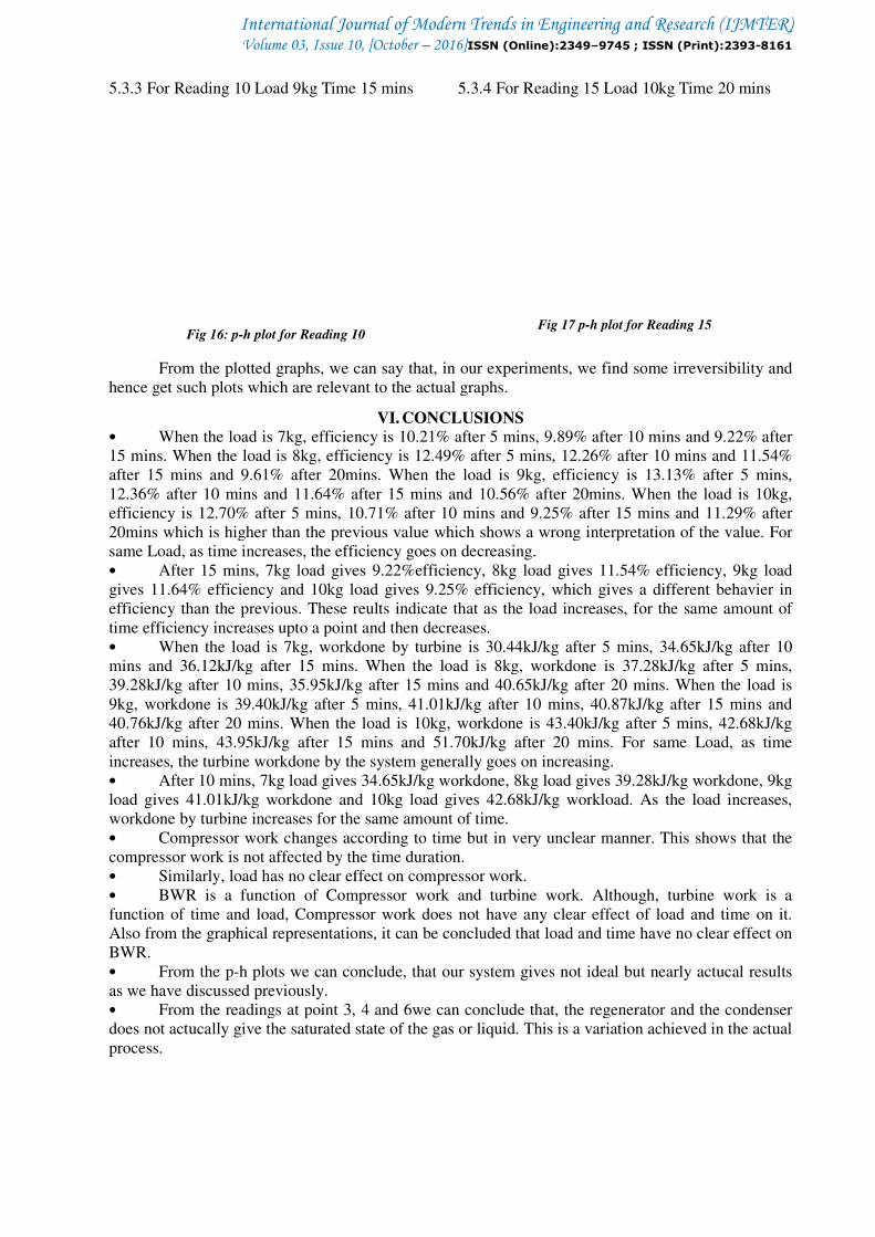
5.3.3 For Reading 10 Load 9kg Time 15 mins
Fig 16: p-h plot for Reading 10
From the plotted graphs, we can say that, in our experiments, we find some irreversibility and
hence get such plots which are relevant to the actual graphs.
• When the load is 7kg, efficiency is 10.21% after 5 mins, 9.89% after 10 mins and 9.22% after
15 mins. When the load is 8kg, efficiency is 12.49% after 5 mins, 12.26% after 10 mins and 11.54%
after 15 mins and 9.61% after 20mins. When the load is 9kg, efficiency is 13.13% after 5 mins,
12.36% after 10 mins and 11.64% after 15 mins and 10.56% after 20mins. When the load is 10kg,
efficiency is 12.70% after 5 mins, 10.71% after 10 mins and 9.25% after 15 mins and
20mins which is higher than the previous value which shows a wrong interpretation of the value. For
same Load, as time increases, the efficiency goes on decreasing.
• After 15 mins, 7kg load gives 9.22%efficiency, 8kg load gives 11.54% efficienc
gives 11.64% efficiency and 10kg load gives 9.25% efficiency, which gives a different behavier in
efficiency than the previous. These reults indicate that as the load increases, for the same amount of
time efficiency increases upto a point and
• When the load is 7kg, workdone by turbine is 30.44kJ/kg after 5 mins, 34.65kJ/kg after 10
mins and 36.12kJ/kg after 15 mins. When the load is 8kg, workdone is 37.28kJ/kg after 5 mins,
39.28kJ/kg after 10 mins, 35.95kJ/kg after 15 mins and 4
9kg, workdone is 39.40kJ/kg after 5 mins, 41.01kJ/kg after 10 mins, 40.87kJ/kg after 15 mins and
40.76kJ/kg after 20 mins. When the load is 10kg, workdone is 43.40kJ/kg after 5 mins, 42.68kJ/kg
after 10 mins, 43.95kJ/kg after 15 mins and 51.70kJ/kg after 20 mins. For same Load, as time
increases, the turbine workdone by the system generally goes on increasing.
• After 10 mins, 7kg load gives 34.65kJ/kg workdone, 8kg load gives 39.28kJ/kg workdone, 9kg
load gives 41.01kJ/kg workdone and 10kg load gives 42.68kJ/kg workload. As the load increases,
workdone by turbine increases for the same amount of time.
• Compressor work changes according to time but in very unclear manner. This shows that the
compressor work is not affected by the time duration.
• Similarly, load has no clear effect on compressor work.
• BWR is a function of Compressor work and turbine work. Although, turbine work is a
function of time and load, Compressor work does not have any clear effect of load and time
Also from the graphical representations, it can be concluded that load and time have no clear effect on
BWR.
• From the p-h plots we can conclude, that our system gives not ideal but nearly actucal results
as we have discussed previously.
• From the readings at point 3, 4 and 6we can conclude that, the regenerator and the condenser
does not actucally give the saturated state of the gas or liquid. This is a variation achieved in the actual
process.
International Journal of Modern Trends in Engineering and Research (IJMTER)10, [October – 2016]ISSN (Online):2349–9745 ; ISSN (Print):2393
ing 10 Load 9kg Time 15 mins
h plot for Reading 10
5.3.4 For Reading 15 Load 10kg Time 20 mins
Fig 17 p-h plot for Reading 1
From the plotted graphs, we can say that, in our experiments, we find some irreversibility and
are relevant to the actual graphs.
VI. CONCLUSIONS
When the load is 7kg, efficiency is 10.21% after 5 mins, 9.89% after 10 mins and 9.22% after
15 mins. When the load is 8kg, efficiency is 12.49% after 5 mins, 12.26% after 10 mins and 11.54%
9.61% after 20mins. When the load is 9kg, efficiency is 13.13% after 5 mins,
12.36% after 10 mins and 11.64% after 15 mins and 10.56% after 20mins. When the load is 10kg,
efficiency is 12.70% after 5 mins, 10.71% after 10 mins and 9.25% after 15 mins and
20mins which is higher than the previous value which shows a wrong interpretation of the value. For
same Load, as time increases, the efficiency goes on decreasing.
After 15 mins, 7kg load gives 9.22%efficiency, 8kg load gives 11.54% efficienc
gives 11.64% efficiency and 10kg load gives 9.25% efficiency, which gives a different behavier in
efficiency than the previous. These reults indicate that as the load increases, for the same amount of
time efficiency increases upto a point and then decreases.
When the load is 7kg, workdone by turbine is 30.44kJ/kg after 5 mins, 34.65kJ/kg after 10
mins and 36.12kJ/kg after 15 mins. When the load is 8kg, workdone is 37.28kJ/kg after 5 mins,
39.28kJ/kg after 10 mins, 35.95kJ/kg after 15 mins and 40.65kJ/kg after 20 mins. When the load is
9kg, workdone is 39.40kJ/kg after 5 mins, 41.01kJ/kg after 10 mins, 40.87kJ/kg after 15 mins and
40.76kJ/kg after 20 mins. When the load is 10kg, workdone is 43.40kJ/kg after 5 mins, 42.68kJ/kg
kJ/kg after 15 mins and 51.70kJ/kg after 20 mins. For same Load, as time
increases, the turbine workdone by the system generally goes on increasing.
After 10 mins, 7kg load gives 34.65kJ/kg workdone, 8kg load gives 39.28kJ/kg workdone, 9kg
kJ/kg workdone and 10kg load gives 42.68kJ/kg workload. As the load increases,
workdone by turbine increases for the same amount of time.
Compressor work changes according to time but in very unclear manner. This shows that the
ted by the time duration.
Similarly, load has no clear effect on compressor work.
BWR is a function of Compressor work and turbine work. Although, turbine work is a
function of time and load, Compressor work does not have any clear effect of load and time
Also from the graphical representations, it can be concluded that load and time have no clear effect on
h plots we can conclude, that our system gives not ideal but nearly actucal results
dings at point 3, 4 and 6we can conclude that, the regenerator and the condenser
does not actucally give the saturated state of the gas or liquid. This is a variation achieved in the actual
and Research (IJMTER) 9745 ; ISSN (Print):2393-8161
For Reading 15 Load 10kg Time 20 mins
h plot for Reading 15
From the plotted graphs, we can say that, in our experiments, we find some irreversibility and
When the load is 7kg, efficiency is 10.21% after 5 mins, 9.89% after 10 mins and 9.22% after
15 mins. When the load is 8kg, efficiency is 12.49% after 5 mins, 12.26% after 10 mins and 11.54%
9.61% after 20mins. When the load is 9kg, efficiency is 13.13% after 5 mins,
12.36% after 10 mins and 11.64% after 15 mins and 10.56% after 20mins. When the load is 10kg,
efficiency is 12.70% after 5 mins, 10.71% after 10 mins and 9.25% after 15 mins and 11.29% after
20mins which is higher than the previous value which shows a wrong interpretation of the value. For
After 15 mins, 7kg load gives 9.22%efficiency, 8kg load gives 11.54% efficiency, 9kg load
gives 11.64% efficiency and 10kg load gives 9.25% efficiency, which gives a different behavier in
efficiency than the previous. These reults indicate that as the load increases, for the same amount of
When the load is 7kg, workdone by turbine is 30.44kJ/kg after 5 mins, 34.65kJ/kg after 10
mins and 36.12kJ/kg after 15 mins. When the load is 8kg, workdone is 37.28kJ/kg after 5 mins,
0.65kJ/kg after 20 mins. When the load is
9kg, workdone is 39.40kJ/kg after 5 mins, 41.01kJ/kg after 10 mins, 40.87kJ/kg after 15 mins and
40.76kJ/kg after 20 mins. When the load is 10kg, workdone is 43.40kJ/kg after 5 mins, 42.68kJ/kg
kJ/kg after 15 mins and 51.70kJ/kg after 20 mins. For same Load, as time
After 10 mins, 7kg load gives 34.65kJ/kg workdone, 8kg load gives 39.28kJ/kg workdone, 9kg
kJ/kg workdone and 10kg load gives 42.68kJ/kg workload. As the load increases,
Compressor work changes according to time but in very unclear manner. This shows that the
BWR is a function of Compressor work and turbine work. Although, turbine work is a
function of time and load, Compressor work does not have any clear effect of load and time on it.
Also from the graphical representations, it can be concluded that load and time have no clear effect on
h plots we can conclude, that our system gives not ideal but nearly actucal results
dings at point 3, 4 and 6we can conclude that, the regenerator and the condenser
does not actucally give the saturated state of the gas or liquid. This is a variation achieved in the actual

International Journal of Modern Trends in Engineering and Research (IJMTER) Volume 03, Issue 10, [October – 2016]ISSN (Online):2349–9745 ; ISSN (Print):2393-8161
@IJMTER-2016, All rights Reserved 68
• Similarly, entropy at point 1 and 2 i.e turbine inlet and outlet is defferent. This occurs because
of the different readings of pressures and temperatures
• We can see a pressure drop or rise in the evaporator or the condenser which again is a heat loss
occurred due to the non-ideal process.
• The results indicate that, out of total waste or exhaust heat, some amount of heat is being
recovered. From this, we can conclude that by using ORC, overall efficiency of the Diesel engine and
the ORC setup combined is increased and due to this, fuel consumption can be reduced.
Acknowledgment Authors acknowledge the Department of Mechanical Engineering of MCT’s Rajiv Gandhi
Institute of Technology and the University of Mumbai, Dr. R.V. Kale for giving us the opportunity to
do this project and “Jadhav Engineering Works” for helping in fabrication of the setup. Mr. Shashank
Shetty and Ms. Amruta Gokhale thank to Dr. Sanjay U. Bokade for helping and guiding throughout
the project.
REFERENCES
[1] Sylvain Quoilin, Martijn Van Den Broek, Se ´Bastien Declaye, Pierre Dewallef, Vincent LeMort, “Techno-economic
Survey Of Organic Rankine Cycle (ORC) Systems”, ELSEVIER- Renewable And Sustainable Energy Reviews 22
(2013) 168-186, 2013.
[2] Tzu-chen Hung, “Waste Heat Recovery Of Organic Rankine Cycle Using Dry Fluids”, Elsevier- Energy Conversion
And Management 42 (2001) 539-553 , 2000.
[3] Jie Zhu and Hulin Huang, “Performance analysis of a cascaded solar Organic Rankine Cycle with superheating”,
International Journal of Low-Carbon Technologies, 2014.
[4] S. Masheiti, B. Agnew and S. Walker “An Evaluation of R134a and R245fa as the Working Fluid in an Organic
Rankine Cycle Energized from a Low Temperature Geothermal Energy Source”, Journal of Energy and Power
Engineering 5 (2011) 392-402. DAVID Publishing. 2011.
[5] Fredy Vélez, Farid Chejne and, Ana Quijano, “Thermodynamic analysis of R134a in an Organic Rankine Cycle for
power generation from low temperature sources”, DYNA, 2014.
[6] J. S. Jadhao, D. G. Thombare, “Review On Exhaust Gas Heat Recovery For I.C. Engine”, International Journal Of
Engineering And Innovative Technology (IJEIT) Volume 2, Issue 12, 2013.
[7] Ngoc Anh Lai, Martin Wendland, Johann Fischer, “Working fluids For High-temperature Organic Rankine Cycles”,
Elsevier- Energy 36 (2011) 199-211, 2010
[8] E.H. Wang, H.G. Zhang, B.Y. Fan, M.G. Ouang, Y. Zhao, Q.H. Mu, “Study Of Working fluid Selection Of Organic
Rankine Cycle (ORC) For Engine Waste Heat Recovery”, ELSEVIER- Energy 36 (2011) 3406-3418, 2011
[9] Fredy Vélez, José, J. Segovia, M. Carmen Martín, Gregorio Antolín, Farid Chejne, Ana Quijanoa, “A Technical,
Economical And Market Review Of Organic Rankine Cycles For The Conversion Of Low-grade Heat For Power
Generation”, Renewable And Sustainable Energy Reviews 16 (2012) 4175-4189, 2012.
[10] M. Chys, M. Van Den Broek,, B. Vanslambrouck, M. De Paepe, ”Potential Of Zeotropic Mixtures As Working fluids
In Organic Rankine Cycles”, Elsevier- Energy 44 (2012) 623-632, 2012.
[11] Lars J. Brasz, William M. Bilbow, “Ranking Of Working Fluids For Organic Rankine Cycle Applications”,
International Refrigeration And Air Conditioning Conference, 2004.
[12] Jamal Nouman, “Comparative Studies And Analyses Of Working Fluids For Organic Rankine Cycles – ORC”, KTH
School Of Industrial Engineering And Management Energy Technology Egi-2012-086msc Division Of
Thermodynamics And Refrigeration Se-100 44 Stockholm, 2012.
[13] M. L. Huber , M. O. McLinden, “Thermodynamic Properties Of R134a (1,1,1,2-tetrafluoroethane)”, International
Refrigeration And Air Conditioning Conference, 1992.
[14] Said Bouazzaoui, Carlos Infante Ferreira, Jürgen Langreck, Jan Gerritsen , “Absorption Resorption Cycle for Heat
Recovery of Diesel Engines Exhaust and Jacket Heat” International Refrigeration and Air Conditioning Conference,
2008
[15] Bala V. Datla , Joost J. Brasz, “Comparing R1233zd And R245fa For Low Temperature ORC Applications ”,
International Refrigeration and Air Conditioning Conference, 2014.