wartsila comments on the august 20, 2014, iepr … 20, 2014 · (track l and 4) as well as...

Tuesday, September 2, 2AL4

Delivered Via Electronic Mailto the Following:

[email protected] i ke.Jaske @en ergy.ca.gov.

California Energy Com mission

Dockets Office, MS-41515 Ninth StreetSacramento, CA 9581 4-55t2

Re: Docket No. 14-lEP-IE

Dear Com missioners Scott:

On behalf of Wdrtsild, N.A. (Wartsil6), we would like to thank you for the opportunity to provide

comments on the California Energy Commission's (CEC)Workshop on "Southern California

Electricity Rel iability."

Given the San Onofre Nuclear Generating Station (SONGS) closure and potentialforthe loss ofseveral megawatts of vintage once-through-cooled (OTC) ocean cooled assets, electric

generating capacity and reliability in Southern California seems to be squarely reliant on the

inter-agency strategy moving forward in conjunction with the efforts of the Investor Owned

Utilities (lOUs) and other load serving entities. With this in mind, WdrtsilS has invested a

serious effort in reviewing the California lndependent System Operator's (CAISO) information

from a system perspective and utilities from an lOU perspective in light of the OTC and SONGS

retirements, in addition to compliance with 33% RPS.

The works (attached) indicate that investment in modular, flexible generation can be quite

helpful in helping California meet CO2 targets, improving reliability, reducing costs and

renewable integration overall. While these works use internal combustion engines (lCEs) as a

proxy for "more flexible generation," the findings are applicable independent of technology

choice, as long as the technologies are actually flexible and cost effective. The analysis

methods used in the attached papers, and the results, are of significance for LTPP proceedings

Wertsile North America, lnc.900 Bestgate Roaderiita ,nn

Tel. i410) 573-2100Eaw. //1 n\ E7a-rrnn

DOCKETEDCalifornia Energy Commission

SEP 04 2014

TN 73734

14-IEP-1E

(Track L and 4) as well as permitting of generation facilities by the CEC. ln particular the works

attached indicate that more flexible simple cycle capacity injected into a portfolio has great

potential for overall system optimization, whereby fleet efficiency is maximized and CO2

generation minimized simultaneously. This is achieved by reduction of cycling and increased

capacity factors of combined cycles, as the flexible units absorb net load fluctuations in the

most cost effective and reliable fashion.

Wdrtsild would like to request that the attached documents and this letter be included in the

official comment record and invite comment/feedback from all interested parties. ln addition,

we would like to recommend that in a future workshop, the CEC strongly consider hosting a

paneldiscussiononthisverysubject. Specifically,areviewofthetechnologiesandortheattributes which would be necessary to achieve system optimization and system reliability

should be reviewed and better understood. While we continue to hearthe terms "fast ramping

technologies," a key questions that should be answered or addressed is 'how do we define such

technology, what does it contribute to system efficiency and reliability, and how is it valued?'

ln advance, thank you for your time and consideration of our request. Should you have any

questions, please feelfree to contact me at 4\O-573-2L0O.

Market Development AnalystWdrtsilii North America, lnc.

900 Bestgate Road, Suite 400Annapolis, MD 214014L0-573-2L00 (office)

443-562-3478 (cell)joseph.ferrari @wa rtsila.com

A WHITE PAPER BY WÄRTSILÄ AND ENERGY EXEMPLAR

INCORPORATING FLEXIBILITY IN UTILITY RESOURCE PLANNING

3

INDEX


Executive summary 41 Introduction and motivation 52 Capacity expansion modeling, past and present 73 Comparing the new and the old 104 Defining the utility 155 New build capacity options for comparison of LDC and Chrono capacity expansion models 166 Comparison of Outcomes from Chronological vs. LDC Capacity Expansion Models 177 Capacity Options – How to Value Increased Diversity and Flexibility 208 Summary and Moving Forward 28

References 31Appendixes1 Information on the Utility used for this Study 322 Transmission Pricing 353 Parameters for Gas-Fired Generation used in Simulations 37

4

EXECUTIVE SUMMARY:

The trend of increasingly variable net load is characteristic of all power systems with increasing penetration of wind and solar energy. As the amount of renewable energy increases, decreasing minimum net loads and increasing net load ramps require more frequent starts and stops, ramps and cycling, all of which impose costs and stress on the dispatchable generation fleet. Operational flexibility is needed to cope with varying net load.

Electric utilities engage in Integrated Resource Planning (IRP) to determine the optimal investments in new generation assets. At the core of IRP efforts are capacity expansion models. These models have historically used a mathematical simplification based on a Load Duration Curve (LDC). The LDC arranges the net load in a simple descending order (e.g., hourly, daily) with no information on ramp events and cycling. As a result, the new capacity selections are not optimized for flexibility needed to meet net load variability. To make up for deficiencies, the typical approach is to apply significant post-analysis approaches, where flexible capacity is added outside of the optimization framework. This implies the resultant fleet is suboptimal, capable of meeting net load fluctuations but at a higher cost than necessary. In this work, we illustrate a state-of-the-art alternative called Chronological modeling, designed to select capacity with the appropriate capabilities in the first place. We then use this approach to quantify the value of flexible capacity as a means to reduce total system costs.

We compare the outcomes of a traditional LDC and Chronological modeling for a utility with aggressive renewable penetration. The traditional approach underestimates annual operational costs by 7%. These errors result in an underestimation of future cost of electricity. Similar errors from the Chronological simulations were less than half that of the LDC approach.

Using the Chronological approach, we compare a base scenario where all new build choices are gas turbines (GT) in simple and combined cycle, versus a flex scenario that includes the same lineup but now adding more flexible options in addition to GT based capacity. By “more flexible” we are referring to capacity options with incremental modularity, faster start times, lower start costs, higher ramp rates and efficiencies. The flex scenario yielded a final buildout that could meet utility load obligations with 9% less capacity and 870 MUSD less cost across the horizon of the analysis. Savings were due primarily to fleet optimization effects, where the full potential of the most efficient units are unlocked as flexible assets attend to net load fluctuations. Detailed dispatch analyses of the fleets (base vs. flex) shows the flex scenario yields 64 MUSD/year operational savings coupled with 1.5% reduction in CO2 emissions.


5

1. INTRODUCTION AND MOTIVATION

Integrated resource planning is a crucial part of long-term planning for utilities, municipalities, electrical cooperatives and national agencies. At the heart of resource planning efforts are capacity expansion models, which solve for the optimal mix of capacity (MW) to install over the next 10, 20 or more years. The optimal solution is the one that presents the least cost and is less sensitive to differences in assumptions than alternatives. Traditionally, this is considered a point in the “efficient frontier”, a careful examination of multiple potential outcomes, with emphasis given towards solutions that provide the lowest cost for an acceptable level of risk.

Capacity Expansion Models (CEMs) are generally found in software packages such as Ventyx Strategist (PROVIEW)™, EPIS AuroraXMP™, SDDP OptGen™, and others. These packages make use of something called the Load Duration Curve (LDC), a mathematical simplification that makes the computational burden of obtaining solutions tractable (Figure 1.1).

Figure 1.1. A typical demand curve profile (A). The raw chronological data by actual hour is sorted from high to low to create the Load Duration Curve (B).

With aggressive penetration of renewable energy, which has accelerated rapidly in the last decade, it is questionable whether the traditional LDC simplification is still valid. To address this potential problem, new software packages, such as Plexos™ are available that use what is called Chronological modeling (Nweke et al. 2012).

Table 1.1. Types of Capacity Expansion Models

Capacity Expansion Model Solves for

Load Duration Curve (LDC) Capacity to meet energy (GWh) needs

Chronological (Chrono) i) Capacity to meet energy (GWh) needs that also has

ii) Capabilities to meet system challenges posed by renewable energy, such as net load ramping

0

1

2

3

4

5

6

7

1 2 3 4 5 6 7 8 9 10 11 12 13 14 15 16 17 18 19 20 21 22 23 24

Pow

er D

eman

d

Actual Hour

A. Hourly Demand Curve

0

1

2

3

4

5

6

7

1 2 3 4 5 6 7 8 9 10 11 12 13 14 15 16 17 18 19 20 21 22 23 24

Pow

er D

eman

d

Sorted High to Low

B. Load Duration CurveA B

6

The goals of this work are to

1. Illustrate the value of Chrono modeling relative to LDC methods (Figure 1.2A).

2. Quantify the value of additional portfolio flexibility using Chrono modeling (Figure 1.2B).

For goal 1 we test the LDC and Chrono models on a target utility with aggressive wind and solar penetration and a reliance on natural gas for capacity expansion. For this exercise we assume gas turbines in simple and combined cycle are the basis of new-build decisions (BASE new build capacity pool) in addition to the renewable expansion.

For goal 2 we use Chrono modeling for the same utility, and compare outcomes using the base capacity pool with outcomes using an alternate flex capacity pool instead. The Flex capacity pool includes all of the gas turbine options in the base, as well as additional technologies with improved dynamic capabilities, i.e. more flexible. By “more flexible” we mean faster starting, faster ramping, lower minimum loads and with greater modularity. The goal is to quantify if Chrono modeling installs greater flexibility (at lower costs) and if so, to explore the mechanisms and quantity by which flexibility brings value.

Figure 1.2. Illustration of the two major comparisons performed in this work.

Utility input data- Existing assets- Retirement schedule- Load growth- Parameters (fuel price, etc.)

Chronological (Chrono)capacity

Expansionmodel

Load Duration Curve (LDC)

capacity Expansion

model

LDC outcomes

GOAL 1

Compare

BASE New build capacity pool

Chronooutcomes

A Utility input data- Existing assets- Retirement schedule- Load growth- Parameters (fuel price, etc.)


expansionmodel

Chronooutcomes

(BASE)

GOAL 2

Compare

BASE New build capacity

pool

Chronooutcomes

(FLEX)

FLEX New build capacity pool


expansionmodel

B

7

2. CAPACITY EXPANSION MODELING, PAST AND PRESENT

Capacity Expansion Models (CEMs) are complex software packages that mathematically determine the optimal, minimum cost buildout of new generation capacity (and in some cases transmission). These programs are necessary because the best solution may not always be obvious. New generation assets are not generally islanded, or isolated – they operate in concert with numerous power stations and in concert with transmission lines from neighboring utilities across which energy is bought and sold. Therefore a CEM solves for assets that minimize the cost of capital and operations for the entire fleet. Cost minimization in this context can mean, for example, recognizing that it may be lower cost to purchase additional energy than it would be to invest in a new power plant and self-generate.

Because CEMs are tasked with solving for time horizons of 10, 20 or more years, they are computationally intensive. Until recently, limitations in computing power constrained the size of the problems that could be solved. Certain simplifications and assumptions were made to simplify the problem and make it more tractable.

Load Duration Curve (LDC): One common simplification is the adoption of the load duration curve (LDC). Loads change throughout the day and seasonally. Historically these load patterns were not dramatically variable, and it was sufficient to approximate them with a mathematical simplification (LDC) which provides all of the information related to the energy needs for the system, while discarding the time dependent nature (chronology) of the load.

The time dependent load for simulation (10, 20+ years) is then “decomposed” into representative blocks (e.g., weekly) across the time horizon and represented within the model with its LDC counterpart. The CEM then solves for the least cost investments (in time) required to meet the energy needs represented by the LDC.

The LDC approach is the basis for most commercially available CEMs. They have been historically successful in maintaining reliable power systems precisely because the assumption of replacing the time dependent, chronological load with an LDC approximation was valid. This was valid because, for the most part, load did not vary substantially hour to hour.

Challenges of renewable integration: Today, however, it cannot be safely assumed that load will behave in such a monotonic fashion (smooth transitions hour to hour). This is true in particular for systems experiencing accelerating growth of renewable energy sources (RES, e.g. wind, solar). Renewable energy sources add complexity to the problem in four ways.

1. Many states/nations have Renewable Portfolio Standards (RPS) that mandate that by a certain date a specific proportion of annual system energy consumed must come from RES.

2. RES are only capable of generating energy when the potential energy they rely on is available – wind turbines only generate when wind is blowing, solar panels only generate when the sun is shining.

3. The potential energy they rely on is variable and not predictable with ultimate certainty. Wind and solar generators can have significant intra-hour variations in output, and although forecasting is able to estimate with some certainty what the output from these units will be, at least on an aggregate level, it is not 100% accurate.

8

4. The variable cost (fuel, operations & maintenance) is close to zero, meaning in market-driven contexts they are assured dispatch. And in some markets, it is legislated that their energy be used first (priority dispatch).

The first point indicates that investment in RES is not subject to traditional mechanisms used to ensure lowest cost delivery of energy. Points 2 and 3 imply that it is not possible to truly schedule and/or dispatch RES in the traditional manner. The last point, low variable cost / priority dispatch, means that the load will first be served by whatever RES energy is available, and the remainder served by truly dispatchable resources (thermal, nuclear, hydro, demand response, storage).

The concept of net load: Items 2, 3, 4 in the list above give rise to the concept of the net load. Load is the true demand that must be served moment by moment. Load is first served by renewable energy, and the remainder is called net load – the load that dispatchable resources must serve – it is at times equal to, but often less than the true load, and it is more variable than the normal load. For systems experiencing aggressive penetration of RES, the difference between load and net load can appear as in Figure 2.1.

Figure 2.1. Illustration of load versus net load for a shoulder month day for a California utility in the year 2022, when the state of California is required to comply with a Renewable Portfolio Standard of 33%.

It is fairly well recognized (e.g. ISO-NE 2010; Lew et al. 2013) that as systems integrate greater amounts of RES such as wind and solar, the following will occur primarily for thermal assets (coal and gas-fired power stations)

• Capacity factors will be reduced, they will run fewer hours and generate less energy serving net load.

• Renewable energy with variable costs approaching zero will drive market prices down, so dispatchable resources will not only run fewer hours, they will be paid less for each MWh they generate.

• Number of starts/stops will increase, adding cost to generation

0

2 000

4 000

6 000

8 000

10 000

12 000

14 000

16 000

18 000

1 2 3 4 5 6 7 8 9 10 11 12 13 14 15 16 17 18 19 20 21 22 23 24

MW

Hour

Dispatchable Generation Renewable Generation

Net Load Load

9

• Cycling and ramping will increase to balance variability in net load.

• Amount of time spent in a part-loaded state and at reduced efficiency will increase (so units can have available ramp capacity to attend to net load fluctuations).

Given this situation, capacity expansion models will often assume a renewable buildout to meet legislated RPS goals and then solve for the least cost buildout of dispatchable resources.

This is where the concerns arise regarding traditional Load Duration Curve approaches. The LDC method does not recognize net load chronology and therefore cannot account for the impacts of a variable net load. These impacts include cycling, part load operation, ramping and starts/stops, all of which impose additional costs, but are not accounted for within the LDC framework. Historically these issues have been addressed outside of the CEM framework, but can they be taken into account already at this fundamental stage?

Chronological modeling: There is at least one alternative to the LDC methodology and it is called Chronological Modeling (Chrono). With Chrono, the optimization algorithms use the raw net load profile instead of decomposing it into a load duration curve. The Chrono method retains all of the information on energy needs of the system in addition to the ramping needs of a variable net load profile.

At present, the only commercially available software that includes both LDC and Chrono approaches for capacity expansion simulations is PLEXOS™. Therefore, using PLEXOS™, we can test the accuracy of the LDC method through comparison with more advanced approaches, such as Chrono, for a system with variable net load.

10

In this section we define the approach used to compare the “New” (Chronological Modeling) versus the “Old” (Load Duration Curve) types of capacity expansion simulations. First, let’s start with the data users have to supply common to both approaches. Input data includes the time period, or horizon. In our case we use 10 years, but it can be set to 20, 30 or more years. For markets where renewable generation is mandated by RPS legislation, we must define renewable buildout (to meet RPS goals) and renewable generation by hour. For all existing assets (thermal plants, wind/solar farms, etc.), information on their size (installed capacity, MW), performance and, if applicable, retirement dates for any assets that are scheduled to go out of service. In addition, projected fuel prices, carbon costs if applicable and any other projections (such as load forecasts) must be defined. Finally, a pool of units and technology types for new build capacity, including details such as build cost ($/kW), efficiency, unit size, etc. is required as input to the model.

The capacity expansion model then employs complex iterative optimization algorithms to determine the least cost solution. Least cost here is defined as the minimum Net Present Value (NPV) of all capital (Capex) and operating (Opex) costs across the 10 year horizon1.

End effects: The NPV also includes end effects. Because assets have economic and technical lifespans, the investment decisions decided in years 1 – 10 will have impacts beyond the last year of the horizon. To account for these “end effects” it is often assumed that when the assets reach the end of their life, they will be replaced in kind at similar costs. The magnitude of the end effect can be quite large and is dependent entirely on the Capex and Opex values in year 10 (Note, we are using a 10 year horizon for illustrative purposes, the same discussion applies to any horizon length, e.g. 20, 30 years).

3. COMPARING THE NEW AND THE OLD

1 An integrated resource plan will typically run a capacity expansion model multiple times across sensitivities in pricing/forecasts, calculate statistical risk/reliability metrics, and generate curves of price ($) vs. risk (e.g. the “Efficient Frontier” plot). In this work, we focus solely on the capacity expansion modeling process (LDC vs. Chrono) and flexibility evaluations, as they are underlying processes for the full integrated resource planning effort.

11

Year Raw values Discounted values

Capex Opex Capex Opex

1 Capex1 Opex1 Capex1D Opex1D










Table 3.1. Capacity Expansion Models determine the types of new generation assets to install, and the associated annualized Capex. New generation is added to the fleet as capacity and then operational costs for the fleet are calculated. Raw values are noted with a subscript noting the year. Final values for each year are then discounted, noted with a subscript noting year as well as the letter “d”. Discounted values are used to calculate Net Present Value of Capex + Opex for the solution.

Discounted annual values are then used in the Net Present Value (NPV) calculation below.

As can be seen from Eq. 2, the end effect is entirely dependent on the last year values for Capex and Opex. As we shall see, the end effect can be quite large, 50% or more of the total NPV. Therefore one gage of the “accuracy” of a capacity expansion model is the extent to which the operational cost used in the CEM is reflective of the true operational costs.

Eq. 1

Eq. 2

12

Use of short-term dispatch modeling to validate the capacity expansion model: How do we know the true operational cost? One estimate of true operational cost is to take the fleet suggested by the CEM for year 10 (last year of horizon) and put it into a detailed dispatch model for load and renewable profiles expected for year 10. Dispatch models differ from capacity expansion models, in that dispatch models are relied on to answer questions on operational costs and unit commitment, typically for much shorter time periods (a month, a year) than capacity expansion model horizons (10, 20+ years). Accordingly dispatch models take more details into account and are generally considered more accurate estimators of operational costs than those obtained from long term capacity expansion models. For example, the LDC method does not retain information on cycling and is therefore unable to account for start costs, whereas a dispatch model retains all of the chronology and explicitly accounts for all start and cycling costs.

To determine which of the two methods is most accurate, we perform capacity expansion modeling on a target utility using both methods (LDC and Chrono) with a common set of inputs, including the types of units considered for new build capacity. Then we compare the operational costs of the fleet buildout in both cases against more accurate estimates obtained using detailed dispatch modeling for the last year of the horizon and calculate and compare error terms (Figure 3.1). The error terms (Eq. 3) are the basis of the comparison for goal 1 (Figure 1.1A).

The error term is calculated as:

Eq. 3

13

Figure 3.1. Flow diagram of comparison approach between Load Duration Curve (LDC) and Chronological (Chrono) capacity expansion models. Model inputs (top block) are representative. Error terms gage the accuracy of the capacity expansion model.

Additional details on model set up:

• Both models (LDC & Chrono) were run using the “LTPlan” module in PLEXOS™

• For both LDC and Chrono modeling in LTPlan, each year was broken into days with 24 (hourly) time blocks. This is a much higher temporal resolution than typically considered (e.g. year broken into weeks with seven daily time blocks).

• For each day the LDC method assigned a load duration curve approximation to the net load, and the Chronological approach used the true net load, retaining the chronology, across the 24 hourly blocks.

Utility Input Data- Existing assets- Retirement schedule- Load growth- Parameters (fuel price, etc.)- Pool of new build capacity

options

LDC Capacity

expansionmodel

ChronologicalCapacity

expansionmodel

Asset fleet (Year 10)

Asset fleet (Year 10)

Detailed annual

dispatch model

LDC Opex

(year 10)

Chrono Opex

(year 10)

Detailed annual

dispatch model

True Opex

(year 10)

True Opex

(year 10)

CompareLDC error term

Chronoerror term

14

• Hourly dispatch modeling was performed on the fleet suggested by each (LDC & Chrono) for the last year of the horizon using the “ST Schedule” module in PLEXOS™

• Each simulation was performed using Mixed Integer Programming, which implies that capacity can only be installed in increments of unit sizes. So, for example, if 50 and 100 MW gas turbines are among the options and the capacity need is for 75 MW, the program must choose two 50 MW units or one 100 MW unit.

• The maximum amount of new-build combined cycle assets was limited to 55% of new build capacity, which matches historical buildouts of utilities in the proximity of the target utility (described below).

• A capacity reserve margin of 15.1% was imposed; for each year of the horizon, the firm capacity installed had to be 15.1% higher than the peak load for that year. This is in line with a typical NERC (National Electric Reliability Council) recommended reserve margin of 15%.

• Capacity reserve margins were assessed relative to “firm capacities”, defined in the following chapter.

The target utility is described in Chapter 4. The types of units considered as common input for the comparison of LDC vs. Chronological modeling are discussed in Chapter 5.

15

4. DEFINING THE UTILITY

We chose an Investor Owned Utility (IOU) indicative of a large western US utility that is experiencing modest load growth, an aggressive renewable buildout based on legislated Renewable Portfolio Standards, low gas prices, and retirement of aging boiler plants, similar in size and facing challenges utilities face in and around the California market. To define this utility, we leaned on the 2012 California Public Utility Commission (CPUC) / California Independent System Operator (CAISO) Long Term Planning and Procurement (LTPP) database. This database is a modified form of the 2012 Western Electricity Coordinating Council (WECC) model. The 2012 LTPP database is a large database/PLEXOS™ model used by researchers, government agencies and consultants (e.g. CAISO 2013; Kema 2013; Lew et al. 2013; E3 2014a) to evaluate renewable integration and information on capacity expansion planning into the future (specifically the 2012 model provides information for the year 2022). This model includes detailed information on every power plant in the entire western United States, including size (MW), efficiency (full and part load), minimum loads, minimum run and down times, ramp rates, etc. as well as information on the utility to which it belongs or is associated with.

This information allowed us to “extract” the assets of an investor owned utility from the database to use as the basis of this study. The intent of this study is to use the utility as a basis for evaluation of the questions posed in this work, not to create a suggested course of action for a specific utility. Therefore the “target utility”, or “the utility” used here, even though based on real world data, is only a proxy for the case analysis.

The utility has an installed capacity in the 1st year of the evaluation of approximately 26 GW. Load growth and peak demand growth are approximately 1.2% per year. Approximately 6 GW of retirements occur across the 10 year horizon, with the majority (@ 5 GW) occurring in the year 2021. Renewables are in the range of 7 GW in 2013, increasing to 11.5 GW by 2022 (40% wind, 60% solar). In addition, the utility has over 9 GW of transmission capacity connecting it to neighboring utilities. Details on the capacity, retirement schedule, etc. are included in Appendix 1. Details on how transmission was modeled are in Appendix 2. An example of net load challenges the utility will face in 2022 is shown in Figure 2.1, which shows a 6 GW net load ramp across 1 hour.

16

5. NEW BUILD CAPACITY OPTIONS FOR COMPARISON OF LDC AND CHRONO CAPACITY EXPANSION MODELS

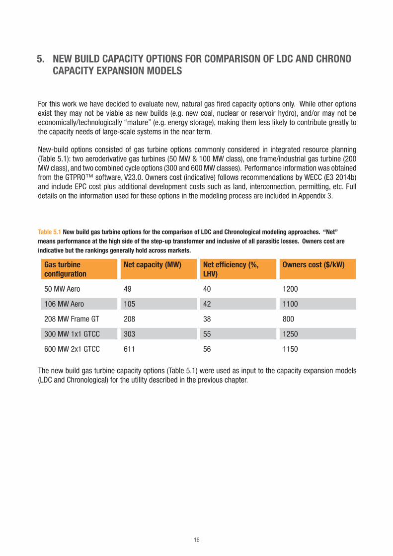
For this work we have decided to evaluate new, natural gas fired capacity options only. While other options exist they may not be viable as new builds (e.g. new coal, nuclear or reservoir hydro), and/or may not be economically/technologically “mature” (e.g. energy storage), making them less likely to contribute greatly to the capacity needs of large-scale systems in the near term.

New-build options consisted of gas turbine options commonly considered in integrated resource planning (Table 5.1): two aeroderivative gas turbines (50 MW & 100 MW class), one frame/industrial gas turbine (200 MW class), and two combined cycle options (300 and 600 MW classes). Performance information was obtained from the GTPRO™ software, V23.0. Owners cost (indicative) follows recommendations by WECC (E3 2014b) and include EPC cost plus additional development costs such as land, interconnection, permitting, etc. Full details on the information used for these options in the modeling process are included in Appendix 3.

Table 5.1 New build gas turbine options for the comparison of LDC and Chronological modeling approaches. “Net” means performance at the high side of the step-up transformer and inclusive of all parasitic losses. Owners cost are indicative but the rankings generally hold across markets.

Gas turbine configuration

Net capacity (MW) Net efficiency (%, LHV)

Owners cost ($/kW)

50 MW Aero 49 40 1200

106 MW Aero 105 42 1100

208 MW Frame GT 208 38 800

300 MW 1x1 GTCC 303 55 1250

600 MW 2x1 GTCC 611 56 1150

The new build gas turbine capacity options (Table 5.1) were used as input to the capacity expansion models (LDC and Chronological) for the utility described in the previous chapter.

17

6. COMPARISON OF OUTCOMES FROM CHRONOLOGICAL VS. LDC CAPACITY EXPANSION MODELS

Capacity buildout and NPV costs from both methods: Due to retirement of steam turbine assets later in the horizon and a modest peak load growth, no new builds were proposed by either modeling approach until the year 2019. The Chrono method proposed installation of greater amounts of capacity (Figure 6.1, table 6.1) and also indicated higher NPV costs (10 year horizon plus end effects) than proposed by the LDC method (Table 6.2).

Figure 6.1. Capacity installed by type, year and method (LDC vs. Chrono)

Table 6.1 Capacity installed by type, LDC and Chrono models

MW Installed LDC Chrono Difference

GTCC 3358 3358 -

GT Ind 2704 2912 208

GT Aero (50MW) - 49 49

GT Aero (100 MW) 105 420 315

Total MW installed 6167 6739 572

Table 6.2 NPV values for each method.

NPV (BUSD) LDC Chrono Difference

Opex 48.4 49.6 1.2

Capex 4.1 4.4 0.4

NPV total cost from LT plan 52.5 54.0 1.5

0

1000

2000

3000

4000

5000

6000

2019 2020 2021 2022

Cap

acity

inst

alle

d by

typ

e (M

W)

100 MW Aero GT

50 MW Aero GT

200 MW Ind GT

GTCC

18

The LDC approach is solving a simplified representation of a variable net load profile that results from substantial amounts of renewable energy. The Chronological method recognizes net load ramping challenges and installs a greater amount of capacity of a different mix that results in a higher cost than the portfolio proposed by the LDC method. The question remains which one is truly more accurate?

Influence of end effect: Recall that the NPV calculation is composed of the sum of 10 year NPV values for Capex and Opex (Eq. 1), with the addition of end effects (Eq. 2). The composition of elements for each of the NPV values indicated Opex accounted for more than 90% of the total NPV, and Opex end effect accounted for 50% of the total NPV.

CAPEX 10 year sum

CAPEX End Effect

OPEX 10 year sum

OPEX End Effect

Figure 6.2 Individual components of total NPV value. Values were equivalent (with marginal differences) for both LDC and Chrono methods.

Since Opex is the major influence on final NPV values, it is necessary to evaluate how accurate the Opex values are. Instead of evaluating Opex for every year subject to different capacities based on retirements and resource additions, a value for the year which has the most influence on NPV, namely the 10th year Opex was analyzed. This is the final year of the horizon in which all retirements have occurred and all new capacities are built, and it is the single value which most influences the magnitude of Opex end effect.

In order to evaluate Opex for the last year, we took the final fleet buildouts (from LDC and Chrono model results) and used them as input to an hourly dispatch model in PLEXOS™. Hourly dispatch models include far more detail than considered in operational cost calculations of capacity expansion models, including the Chrono method. Therefore, one measure of the accuracy of a capacity expansion model is the degree to which the resulting Opex values align with Opex values determined from a dispatch model.

Error terms from Eq. 3 (Table 6.3) indicate the 10th year Opex in the LDC method underestimated true operational costs by 7% compared to 3% for the Chrono method. Errors for both methods imply that the capacity expansion model will underestimate the total NPV. These errors are inescapable, an artifact of the underlying assumptions in the capacity expansion models. However, if different models are available, the one with the smallest error terms should be chosen. This is especially relevant in long term planning results that base end effects on Opex values from the last year of the horizon.

19

These results support the concept that the Chronological method is a better approach for systems with heavy renewable penetration and variable net loads. Because the Chrono method retains information on time development of net loading, it installs capacity that has the requisite capabilities to meet net load ramps, as evidenced by the smaller error terms for the Chrono method. Because the magnitude of the error is smaller with the Chrono method, the overall NPV values (dominated by Opex) can also be considered to be more robust and realistic relative to LDC approaches. In other words, the LDC method underestimates the capacity and capability needed and ultimately underestimates the operational costs of the utility portfolio. If this would be the sole determinant of the portfolio planning, the utility would not select the optimal portfolio mix and the cost of energy to the ratepayer would not be based on the optimal solution.

Table 6.3 Comparison of Opex from dispatch simulation results and from capacity expansion models for the year 2022.

Dispatch model results (BUSD) LDC Chrono

Fuel + VOM + CO2 + start costs 2.77 2.74

Import (cost) 0.08 0.08

Export (revenue) 0.74 0.73

Total dispatch model opex 3.58 3.55

Opex from capacity expansion model 3.34 3.45

Error term (Eq. 3), % 7 3

20

7. CAPACITY OPTIONS – HOW TO VALUE INCREASED DIVERSITY AND FLEXIBILITY

Now that we have determined that the Chrono method is most appropriate for systems with a variable net load influenced by renewable energy sources, we can move to the next question. Given that these systems require assets that can best handle low net loads and large net load ramps, how would a more diverse and capable fleet of resources influence costs? Specifically, if the traditional pool of gas turbine based choices for capacity expansion were expanded to include additional generation types, how would the outcome (fleet buildout, NPV) of a Chronological capacity expansion model differ?

Alternate flexible options for gas fired capacity: To test the questions posed above, we considered additional options (Table 7.1) based on natural gas-fired, internal combustion engines (hereafter referred to as ICE). Full details on the information used for these options in the modeling process are included in Appendix 3.

Features of modern (specifically medium-speed, 500-800 rpm) internal combustion engines include:

• Modular (10 to 20 MW per unit) capacity for projects up to 500 MW or more

• Highest simple cycle efficiency (46–48% depending on engine model).

• Very high part-load efficiency

• Insensitive to temperature: no derate on output/efficiency until > 100°F/38°C

• Insensitive to altitude: no derate on output/efficiency until > 5000 ft/1500 m

• Minimum stable loads of 30% (per engine), as low as 1% of plant load for a large multi-engine facility

• Operational ramp rates of 100% per minute or more (from min stable to full load in < 1 min)

• Fast start (0 to full load) in < 5 minutes, MW to grid in 30s

• High reliability and availability

• No minimum run time

• Minimum down times of 5 minutes

• Unrestricted number of starts/stops per day with no impact on cost or maintenance

• Automatic Generation Control (AGC), remote dispatch and black start capability

• No process water consumption due to usage of closed loop radiator cooling

• Proven technology, power plant applications worldwide, with decades of experience. Wärtsilä, the leading supplier, has over 55 GW of power plant references, 2.7 GW in the USA.

21

Table 7.1 New build internal combustion engine options. “Net” means performance at the high side of the step-up transformer and inclusive of all parasitic losses. Owners cost are indicative but the rankings generally hold across markets.

Internal combustion engine configuration

Plant net capacity (MW) Net efficiency (%, LHV) Owners cost ($/kW)

10 MW class units 50+ 44% 1150

20 MW class units 100+ 45% 1100

Base and Flex capacity pools: A comparison is then made between Chrono capacity expansion modeling outcomes using the Base and Flex alternative pools of new-build capacity options. From the previous comparison (LDC vs. Chrono) the results for the Base pool are the same as the results for the Chrono method in the previous section. Therefore, for this comparison, the only additional simulation needed is to run the same Chrono capacity expansion model, only this time using the Flex capacity pool. Note that the Flex pool includes all of the gas turbine based options in the Base, with the primary difference being the inclusion of two internal combustion engine alternatives.

For this second part of the study, the utility was analyzed using the Chrono capacity expansion model, under two scenarios; BASE and FLEX. The BASE scenario uses the Base capacity pool, and the FLEX scenario uses the Flex capacity pool. Final NPV values and operational aspects of the suggested fleets from the scenario outcomes are compared (Figure 7.1).

22

Figure 7.1 Comparison of outcomes from Chronological capacity expansion model using two different new build capacity pools. The BASE scenario is based on gas turbine units only (Base capacity pool). The FLEX scenario uses all units considered in the Base capacity pool plus two additional combustion engine units.

Utility Input Data- Existing assets- Retirement schedule- Load growth- Parameters (fuel price, etc.)

Chronologicalcapacity

Expansionmodel

Asset fleet / BASE

(Year 10)

Chronologicalcapacity

Expansionmodel

BASE New build capacity

pool

FLEXNew build capacity

pool

BASE NPV

Asset fleet / FLEX

(Year 10)

FLEXNPV

Dispatch model

BASE OPEX

FLEX OPEX

Compare

Compare

Dispatch model

23

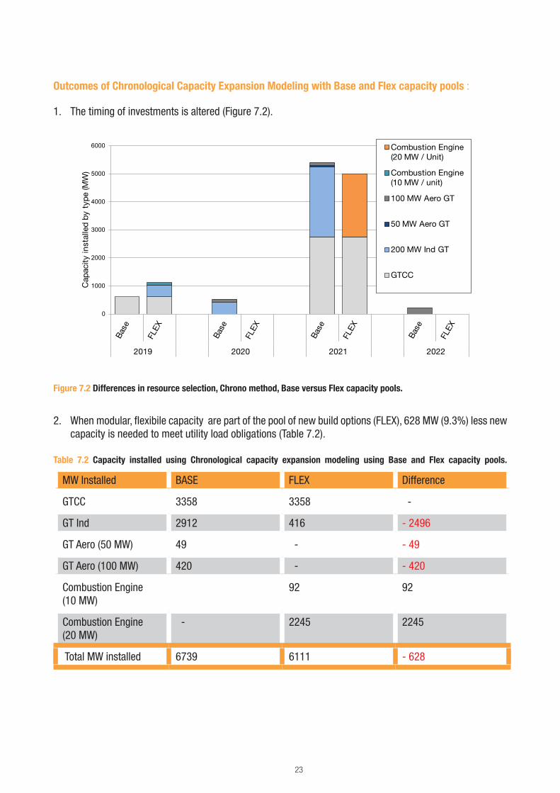
Outcomes of Chronological Capacity Expansion Modeling with Base and Flex capacity pools :

1. The timing of investments is altered (Figure 7.2).

Figure 7.2 Differences in resource selection, Chrono method, Base versus Flex capacity pools.

2. When modular, flexibile capacity are part of the pool of new build options (FLEX), 628 MW (9.3%) less new capacity is needed to meet utility load obligations (Table 7.2).

Table 7.2 Capacity installed using Chronological capacity expansion modeling using Base and Flex capacity pools.

MW Installed BASE FLEX Difference

GTCC 3358 3358 -

GT Ind 2912 416 - 2496

GT Aero (50 MW) 49 - - 49

GT Aero (100 MW) 420 - - 420

Combustion Engine (10 MW)

92 92

Combustion Engine (20 MW)

- 2245 2245

Total MW installed 6739 6111 - 628

0

1000

2000

3000

4000

5000

6000

2019 2020 2021 2022

Cap

acity

inst

alle

d by

typ

e (M

W)

Combustion Engine (20 MW / Unit)

Combustion Engine (10 MW / unit)

100 MW Aero GT

50 MW Aero GT

200 MW Ind GT

GTCC

24

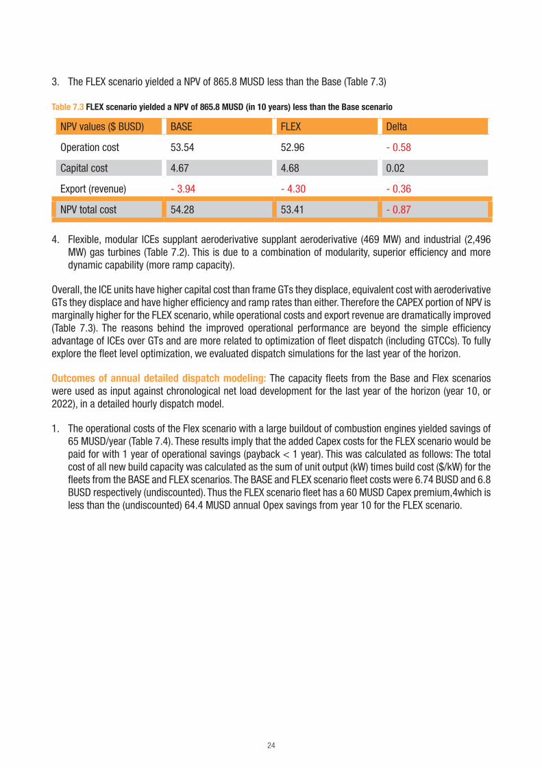
3. The FLEX scenario yielded a NPV of 865.8 MUSD less than the Base (Table 7.3)

Table 7.3 FLEX scenario yielded a NPV of 865.8 MUSD (in 10 years) less than the Base scenario

NPV values ($ BUSD) BASE FLEX Delta

Operation cost 53.54 52.96 - 0.58

Capital cost 4.67 4.68 0.02

Export (revenue) - 3.94 - 4.30 - 0.36

NPV total cost 54.28 53.41 - 0.87

4. Flexible, modular ICEs supplant aeroderivative supplant aeroderivative (469 MW) and industrial (2,496 MW) gas turbines (Table 7.2). This is due to a combination of modularity, superior efficiency and more dynamic capability (more ramp capacity).

Overall, the ICE units have higher capital cost than frame GTs they displace, equivalent cost with aeroderivative GTs they displace and have higher efficiency and ramp rates than either. Therefore the CAPEX portion of NPV is marginally higher for the FLEX scenario, while operational costs and export revenue are dramatically improved (Table 7.3). The reasons behind the improved operational performance are beyond the simple efficiency advantage of ICEs over GTs and are more related to optimization of fleet dispatch (including GTCCs). To fully explore the fleet level optimization, we evaluated dispatch simulations for the last year of the horizon.

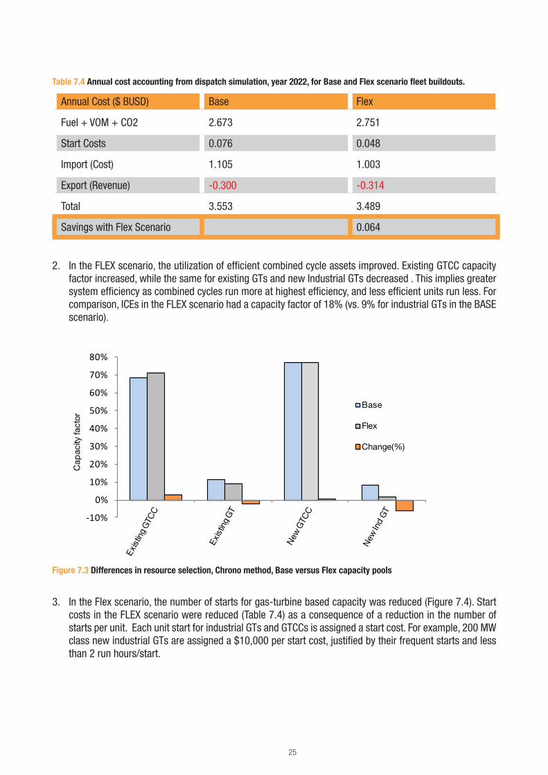
Outcomes of annual detailed dispatch modeling: The capacity fleets from the Base and Flex scenarios were used as input against chronological net load development for the last year of the horizon (year 10, or 2022), in a detailed hourly dispatch model.

1. The operational costs of the Flex scenario with a large buildout of combustion engines yielded savings of 65 MUSD/year (Table 7.4). These results imply that the added Capex costs for the FLEX scenario would be paid for with 1 year of operational savings (payback < 1 year). This was calculated as follows: The total cost of all new build capacity was calculated as the sum of unit output (kW) times build cost ($/kW) for the fleets from the BASE and FLEX scenarios. The BASE and FLEX scenario fleet costs were 6.74 BUSD and 6.8 BUSD respectively (undiscounted). Thus the FLEX scenario fleet has a 60 MUSD Capex premium,4which is less than the (undiscounted) 64.4 MUSD annual Opex savings from year 10 for the FLEX scenario.

25

Table 7.4 Annual cost accounting from dispatch simulation, year 2022, for Base and Flex scenario fleet buildouts.

Annual Cost ($ BUSD) Base Flex

Fuel + VOM + CO2 2.673 2.751

Start Costs 0.076 0.048

Import (Cost) 1.105 1.003

Export (Revenue) -0.300 -0.314

Total 3.553 3.489

Savings with Flex Scenario 0.064

2. In the FLEX scenario, the utilization of efficient combined cycle assets improved. Existing GTCC capacity factor increased, while the same for existing GTs and new Industrial GTs decreased . This implies greater system efficiency as combined cycles run more at highest efficiency, and less efficient units run less. For comparison, ICEs in the FLEX scenario had a capacity factor of 18% (vs. 9% for industrial GTs in the BASE scenario).

Figure 7.3 Differences in resource selection, Chrono method, Base versus Flex capacity pools

3. In the Flex scenario, the number of starts for gas-turbine based capacity was reduced (Figure 7.4). Start costs in the FLEX scenario were reduced (Table 7.4) as a consequence of a reduction in the number of starts per unit. Each unit start for industrial GTs and GTCCs is assigned a start cost. For example, 200 MW class new industrial GTs are assigned a $10,000 per start cost, justified by their frequent starts and less than 2 run hours/start.

-10%

0%

10%

20%

30%

40%

50%

60%

70%

80%

Cap

acity

fact

or

Base

Flex

Change(%)

26

Figure 7.4 The number of starts/unit for Base and Flex scenarios. “Change” is the value from Flex minus the value from the Base scenario.

4. In the Flex scenario, the amount of imports was reduced, and the revenue from exports increased. Increased system efficiency coupled with lower start costs yielded a reduced marginal cost of the portfolio for the FLEX scenario, reducing import costs and increasing export revenue (Table 7.4).

The value of flexibility – where do the savings come from: The results of this analysis show that if efficient and flexible capacity is considered in capacity expansion planning above and beyond the traditional gas turbine based capacity, portfolio outcomes will be superior. In this case the flexible alternative evaluated were combustion engines (ICEs). Superior outcomes with ICEs include

• Reduced NPV (including end effects), savings of 866 MUSD in ten years

• Reduced amount of installed capacity, 628 MW less

• Increased fleet efficiency, which

• Reduces marginal costs

• Reduces costs of purchased energy (imports)

• Increases revenue from export energy.

• Dispatch (last year) results show annual operational savings of 65 MUSD/year

• Dispatch results also show a 1.5% reduction in CO2 (for the fleet)

The savings and improvements can be separated into a few broad areas;

1. Portfolio optimization: By injecting more flexible capability with zero (maintenance-based) start costs combined cycle assets can generate at a more stable dispatch that optimizes the fleet generation cost. This may seem counter-intuitive, where it would be easy to assume higher efficiency CE units would decrease the capacity factors of all other units, but this is not the case. Capacity factors of the most efficient units increased while starts decreased. This indirect enhancement is what we term Portfolio optimization.

-150

-100

-50

-

50

100

150

200

250

300 S

tart

s / u

nit

Base

Flex

Change

27

2. Efficiency improvements: Portfolio optimization is manifested by a combination of reduced cycling and increased system efficiency, yielding a reduced marginal cost for the entire portfolio.

3. Improved import/export net balance: The lower marginal cost of the portfolio reduced imports from neighboring providers and increased exports and resulted in the positive portfolio effect.

4. More capital efficient buildout: The smaller increments of the ICE based assets can reduce overbuild situations as they can be tailored to the exact requirements while maintaining economies of scale, e.g. plants can be built for 160 MW or 180 MW with the same cost per kW installed.

5. Less capacity needed: Generally the greater the flexibility of a capacity type, the less capacity needed to meet net load fluctuations (Makarov et al., 2008). In addition, modularity allows for exact matching of capacity needs.

6. CO2 reduction: Dispatch results show that the FLEX fleet generates more GWh, but consumes less fuel than the BASE fleet, reflected by a 1.5% reduction in CO2 emissions. So the portfolio optimization and efficiency improvements show that increased flexibility also reduces the carbon footprint.

28

8. SUMMARY AND MOVING FORWARD

The first goal of this work was to illustrate the value of Chrono modeling over traditional LDC approaches. Comparison of operational costs from Chrono and LDC against a more detailed dispatch model showed that the error terms of the Chrono model were less than half of the LDC method. The reason for the difference is that the LDC approach cannot account for variability in net loading, which can have serious impacts on the dispatchable fleet.

These findings suggest utility resource planners should consider Chrono modeling as an alternative or complement to more traditional methods. If Chrono modeling is infeasible, due to cost and time required to transition from legacy use of LDC to Chrono and/or lack of computing power, detailed dispatch analyses across several scenarios should be used to judge (or modify) NPV outcomes of LDC simulations. The findings have increasing relevance for regions experiencing aggressive renewable penetration coupled with increasing net load variability. As the proportion of renewable energy increases, continued reliance on LDC methods may seriously compromise the validity of financial decisions related to asset acquisition and portfolio costs.

The second goal of this work was to explore how the Chrono method would value greater flexibility. The comparison was made between capacity expansion modeling results using a gas-turbine-centric Base pool of new-build capacity versus the same but including two additional internal combustion engine (ICE) alternatives, which have similar capital costs to gas turbines but are inherently more flexible (modular, fast start, fast ramp, fast shut down etc.). When ICEs were included as an option for the model to select, they supplanted over 2 GW of new build gas turbines, required 628 MW less capacity and yielded a net present value (NPV) savings of 866 MUSD. Although capital costs were higher, dispatch analysis showed the 64 MUSD/year savings in operational costs compared to the additional capital cost of 60 MUSD (non NPV) delivered a payback of less than 1 year.

While this work uses ICEs as a proxy for “more flexible capacity”, the approach illustrated would be equally applicable to any type of capacity including energy storage, distributed generation and demand response. Regardless of the type of capacity considered, this work shows additional flexibility with a minimum premium on capital cost ($/kW) can yield significant fleet-level optimization, reduce fuel use, reduce CO2 generation, reduce marginal costs, increase revenues from exports, and yield significant savings across the entire portfolio.

The engine of change – flexibility: Dispatch modeling of the FLEX scenario was used to show the source of savings on an annual basis related to combined cycle dispatch optimization, start costs, CO2, import/export, etc. These operational savings were relative to the same system evaluated only allowing for gas turbines as new capacity (BASE scenario). Thus the savings were the result of the efficiency, modularity and flexibility of ICEs over GTs.

The value of flexibility that internal combustion engines provide has been explored in some detail in recent operational studies. In particular, Kema (2013), Wärtsilä & Redpoint (2013) and Wärtsilä and Energy Exemplar (2014) have performed dispatch simulations of the United Kingdom and the California Independent System Operator (CAISO) power systems in future years when renewable sources are expected to supply 30% or more of the energy needs. In all 3 studies, when combustion engines were introduced to the resource mix, significant operational savings were achieved (4–12% annually).

29

The mechanisms that contributed to the operational/system savings were the same as evidenced in this work for the FLEX scenario; optimization of GTCC dispatch, reduction of number of starts, increase in system efficiency, and reduction of CO2 generation and costs. These prior system studies did not include the impact of capital costs, instead they compared outcomes with different portfolios that included internal combustion engines as part of the capacity mix against a baseline scenario of planned gas turbine-based capacity additions. The assumption was that all gas-fired assets are somewhat similar in capital costs so the savings quantified are true operational savings based on two separate resource plans with similar capital costs. This current work is aimed at also including the capital cost issue directly in the evaluation, while also looking at the optimization from the utility portfolio planning point of view, similar to what many utilities perform in their Integrated Resource Planning.

Ancillary services: Ancillary services (operational reserves or contingency reserves) are reserve capacity intended to, among other things, make up any shortfalls. Shortfalls can be caused by a mismatch between scheduled and actual real time operations. For example, between hourly and 5 minute, and between 5 minute and real time markets. These shortfalls are caused by discrepancies between scheduled and actual generation and are exacerbated with greater amounts of renewable energy (e.g. as wind generation has higher variability and uncertainty than thermal generation, the inclusion of wind will increase both these metrics of a portfolio and increase the need for regulation, a primary service for adjustment between 5 minute forecasts and real time). The most expensive ancillary services are “uplift” services, those that require units to run at part load and be available to ramp upwards as needed or as a result of a contingency (e.g. the largest unit in the system trips). The previous operational studies illustrated that when combustion engines make up 6 – 8% of system capacity, they can provide up to 80% of uplift ancillary services at significantly lower costs. This, in turn, frees combined cycles from having to provide these services and allows them to run at their maximum full load efficiency with a minimum number of starts and stops. Based on these prior studies, it is reasonable to expect that fleet buildouts that include superior flexibility will also optimize provision of ancillary services and provide even greater savings than indicated here, which were based solely on energy. Further analysis could include ancillary service requirements in addition to capacity and energy considerations.

The value of modularity: Because internal combustion engines can be installed in capacity blocks of 10 or 20 MW, capacity can be installed to meet projected needs, avoiding the “lumpy investment” issue. Capacity blocks of 10 and 20 MW allow for meeting projected needs without overinvesting. Modularity also provides another advantage from a system benefit perspective. A multi-unit plant can follow loads by cycling units on and off, with no additional start or maintenance costs. In this manner, the majority of units on line are at or near full load, at maximum efficiency and with subsequent minimization of fuel costs and CO2 generation.

Finally, in many areas the cost of new transmission is prohibitive, and congestion on lines can drive up marginal costs significantly. Modular plants allow for custom-sized plants in load pockets that could offset transmission costs for new lines or upgrades and/or alleviate transmission constraints and congestion costs.

Putting it in the context of a full Integrated Resource Plan: Given chronological modeling should complement or replace traditional capacity expansion models, resource planners should take advantage of all commercially viable potential candidates for new builds during their evaluations. This requires moving beyond the traditional mix of gas turbines in simple and combined cycle. This work highlights one such candidate, internal combustion engines and demonstrates the substantial savings that could be achieved mainly through fleet optimization effects. However, full integrated resource plans (IRPs) also have to consider other factors such as reliability and sensitivity to risks (such as deviance in hydrology, weather, fuel or load forecasts).

30

Smaller sized generating units will result in greater reliability (Biewald & Bernow 1988). Multi-unit ICE plants are based on increments of 10 or 20 MW, smaller than typical GT unit sizes. Low forced outage rates also increase reliability, and these rates for ICEs are in the range of 1% per unit, less than that for most gas turbines on a per-unit basis. As an example, a 10 x 20MW ICE plant would have a forced outage rate (for all 200 MW) of 1% to the 10th power. Compared to a 200 MW industrial GT the forced outage rate of the 200 MW ICE plant is literally orders of magnitude lower. Small incremental unit sizes and low forced outage rates for utility scale ICE plants will increase system reliability and consequently, decrease the reserve margin necessary to meet reliability standards.

In terms of sensitivities, simple logic would show that if fuel price increased, preference would be given to the most efficient simple cycle units (ICEs). If renewable energy became more volatile, preference in the simple cycle space would be given to units with the highest ramp rates (ICEs) and highest part load efficiency (ICEs).

Utilities must also work towards legislative goals, such as minimization of greenhouse gases (such as CO2). This work and several earlier (operational) studies all show that enhanced flexibility increases system efficiency and reduces CO2 emissions (and costs). Thus the greater the modularity and flexibility of the fleet, the more able it is to assist in meeting legislative goals and the less sensitive it is to variances in forecasts.

This work demonstrates the value of Chronological capacity expansion planning and shows the value of increased flexibility in resource selection (using Internal Combustion Engines as a proxy for “a more flexible resource”). We hope that this work will stimulate further thought and investigation across the industry, with a goal towards delivering reliable, sustainable and cost-effective energy via investment in the right amounts of capacity with the right capabilities to handle the challenges of renewable integration.

31

Biewald B and S Bernow (1988) Electric Utility System Reliability Analysis: Determining the Need for Generating Capacity. Synapse Energy Economics, Inc. Prepared for the 6th NARUC Biennial Regulatory information conference, Sept. 1, 1988. http://www.synapse-energy.com/Downloads/SynapsePaper.1988-09.0.Reliability-Analysis.A0033.pdf

CAISO (2013) Summary of Preliminary Results of 33% Renewable Integration Study – 2010 CPUC LTPP Docket No. R.10-05-006. http://www.cpuc.ca.gov/NR/rdonlyres/E2FBD08E-727B-4E84-BD98-7561A5D45743/0/LTPP_33pct_initial_results_042911_final.pdf

E3 (Energy+Environmental Economics) (2014a) Investigating a Higher Renewables Portfolio Standard in California. http://www.ethree.com/documents/E3_Final_RPS_Report_2014_01_06_with_appendices.pdf

E3 (Energy+Environmental Economics) (2014b) Capital Cost Review of Generation Technologies- Recommendations for WECC’s 10- and 20-Year Studies, March 2014 29pp. http://www.wecc.biz/committees/BOD/TEPPC/External/2014_TEPPC_Generation_CapCost_Report_E3.pdf

ISO-NE (2010) Final Report: New England Wind Integration Study. http://www.iso-ne.com/committees/comm_wkgrps/prtcpnts_comm/pac/reports/2010/newis_report.pdf

Kema (2013) How to Manage Future Grid Dynamics: Quantifying Smart Power Generation Benefits. Prepared by KEMA, Inc., 2/14/2013. http://www.wartsila.fi/file/Wartsila/en/1278539529030a1267106724867-Wartsila_Smart_Power_Generation_study_by_DNV_KEMA.pdf

Lew D, G Brinkman, E Ibanez, A Florita, et al., (2013) National Renewable Energy Laboratory, Western Wind and Solar Integration Study, Phase 2. http://www.nrel.gov/docs/fy13osti/55588.pdf

Makarov, YV, J Ma, S Lu, TB Nguyen (2008) Assessing the Value of Regulation Resources Based on Their Time Response Characteristics. Pacific Northwest National Laboratories. http://www.pnl.gov/main/publications/external/technical_reports/PNNL-17632.pdf

Nweke CI, F Leanez, GR Drayton, M Kohle (2012) Benefits of Chronological Optimization in Capacity Planning for Electricity Markets. 2012 IEEE International Conference on Power System Technology. http://energyexemplar.com/wp-content/uploads/publications/Nweke%20et%20al_2012.pdf

Wärtsilä (2013). Flexible energy for efficiency and cost effective integration of renewables in power systems. A Wärtsilä white paper supported by modelling conducted by Redpoint Energy, a business of Baringa Partners. http://www.wartsila.com/file/Wartsila/en/1278539529482a1267106724867-Wartsila_Smart_Power_Generation_study_by_Redpoint.pdf

Wärtsilä and Energy Exemplar (2014) Power System Optimization by Increased Flexibility. http://www.wartsila.com/file/Wartsila/en/1278539707069a1267106724867-Wartsila_Power_System_Optimization_White_Paper_2014_with_Energy_Exemplar.pdf

REFERENCES

32

APPENDIX 1 INFORMATION ON THE UTILITY USED FOR THIS STUDY

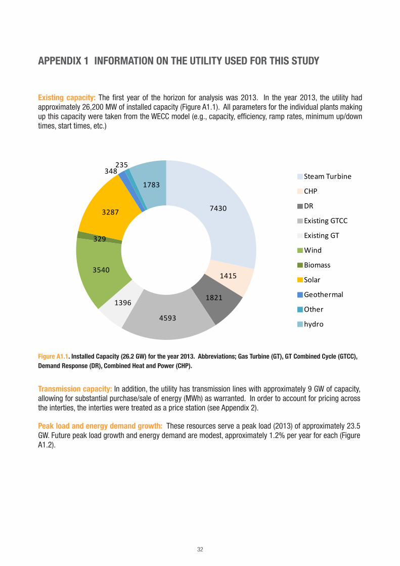
Existing capacity: The first year of the horizon for analysis was 2013. In the year 2013, the utility had approximately 26,200 MW of installed capacity (Figure A1.1). All parameters for the individual plants making up this capacity were taken from the WECC model (e.g., capacity, efficiency, ramp rates, minimum up/down times, start times, etc.)

7430

1415

1821

4593

1396

3540

329

3287

348235

1783Steam Turbine

CHP

DR

Existing GTCC

Existing GT

Wind

Biomass

Solar

Geothermal

Other

hydro

Figure A1.1. Installed Capacity (26.2 GW) for the year 2013. Abbreviations; Gas Turbine (GT), GT Combined Cycle (GTCC), Demand Response (DR), Combined Heat and Power (CHP).

Transmission capacity: In addition, the utility has transmission lines with approximately 9 GW of capacity, allowing for substantial purchase/sale of energy (MWh) as warranted. In order to account for pricing across the interties, the interties were treated as a price station (see Appendix 2).

Peak load and energy demand growth: These resources serve a peak load (2013) of approximately 23.5 GW. Future peak load growth and energy demand are modest, approximately 1.2% per year for each (Figure A1.2).

33

Figure A1.2 Assumed peak load (MW) and energy (GWh) growth 2013 – 2022.

Retirement schedule of existing assets: While existing assets are capable of meeting load at present, challenges are posed by retirement of existing steam, or boiler plants (Figure A1.3). In this specific case, the units are gas-fired and are facing closure due to legislation that bans the use of once-through cooling (e.g. the use of river or coastal waters for heat rejection). They could just as easily be coal-fired boilers facing closure due to economic viability concerns related to low-cost shale gas coupled with compliance costs associated with environmental legislation.

Figure A1.3 Steam turbine power plant retirement schedule 2013 – 2022.

110 000

112 000

114 000

116 000

118 000

120 000

122 000

124 000

126 000

23 000

23 500

24 000

24 500

25 000

25 500

26 000

26 500

2013 2015 2017 2019 2021

Energ

y (GW

h)P

eak

load

(MW

)

Year

Peak Load (MW) Energy (GWh)

0

1000

2000

3000

4000

5000

2013 2014 2015 2016 2017 2018 2019 2020 2021 2022

Cap

acity

(MW

)

Year

34

Scheduled buildout of Renewable Energy Sources (RES) for compliance with Renewable Portfolio Standard (RPS) requirements: The buildout of RES capacity was assumed (Figure A1.4), and considered a) dependent on compliance with RPS legislation and b) independent of economic evaluation or consideration within the context of capacity expansion modeling. The buildout of RES will supply approximately 30% of energy (GWh) for the utility by the year 2020.

Figure A1.4 Scheduled buildout of Renewable Energy Sources (2013-2022).

Firm capacity: While units are commonly defined by their name plate capacity, for the purpose of capacity reserve margins it is necessary to define what is called firm capacity. Here “firm capacity” refers to the availability for the capacity to deliver energy during the hour of annual peak load. If, for example, the peak load occurs at night, the firm capacity of solar is zero.

Table A1.1 Firm capacity ratios for selected technologies

Technology type Firm capacity rating

Thermal 100% of summer rating

Hydro 82%

Biogas 62%

Wind 0.2%

Solar 40–70%, depending on load shape at peak hours

Transmission / Interchange 100%

0

2000

4000

6000

8000

10000

12000

Cap

acity

(MW

)

Year

Wind

Solar

35

APPENDIX 2 TRANSMISSION PRICING

The utility chosen for this work had several transmission lines with an aggregate capacity of approximately 9.5 GW, with the potential to supply a substantial portion of the energy needs. Energy flow into the utility across these lines were considered as costs, while flows outwards were considered sources of revenue. This section describes the basic methodology of how the transmission line pricing was established to inform import/export decisions in the capacity expansion and dispatch simulations.

Recall the data for the utility was taken as a subset of the original Plexos™ 2022 WECC model. The WECC model is a dispatch simulation tool used to evaluate generation within, and energy transfer among, multiple entities (utilities, states, balancing areas) in the broad geographic region which the WECC model encompasses. Within the state of California, each of the major utilities is designated as its own region, with basic transmission represented among them and with other entities (within CAISO, such as large municipalities that manage their own load, or with transmission across state lines).

Therefore, the WECC model can be used as a template for understanding how the utility trades energy across transmission lines. The process by which this was done is described as follows:

1. Run an hourly dispatch simulation for the entire WECC system for the year 2022, using all defined assets within the 2022 WECC model.

2. Acquire the hourly regional power price for the utility and the neighboring areas from that run.

3. Define regional market heat rates for the utility and neighboring areas as the regional power price divided by the fuel (natural gas) price.

4. For each major transmission line capable of importing or exporting energy, within the PLEXOS™ capacity expansion model define a pair of proxy generators, one for import and one for export.

5. Use hourly market heat rate profiles derived in step 3 as the input heat rate for the two proxy generators.

• The export is modeled as a negative generator in PLEXOS.

• In this way, the import and export generators are placed in the supply stack along with other internal resources and PLEXOS will determine whether it is economic to dispatch internal resources or use the import generators.

• PLEXOS will decide when it is economic to use cheaper internal resources to sell the power to the neighbors at a higher price.

6. Because these price stations are only sensitive to the price signal. It is necessary to place a ramp rate to these import/export generators. Otherwise they can move their generation output up and down instantaneously, which is not realistic.

• Historical flow data was evaluated for the maximum observed ramp rates (MW/h, from hour to hour) across transmission lines connecting the utility to neighboring areas.

36

• Regression analysis showed that the maximum observed ramp rate across any line was no more than 1/3 of capacity.

• Therefore a ramp rate limitation was imposed on the generators/price stations, so that the power flow was limited to 1/3 of line capacity hour to hour.

7. The ramp limitations are only applicable to Chronological capacity expansion simulations. In the LDC mode simulation, the chronological constraints are ignored, as is the ramp rate limitation.

8. Imports for any hour were assigned a cost of the MWh purchased times the regional price defined for the hour.

9. Exports for any hour were assigned revenue as the MWh exported times the higher regional price in the neighboring region. Costs (fuel, VOM, CO2, start costs) to supply energy for export are accounted for in Opex separately.

While this method of using price stations to account for import and export of energy is dynamic, it is still based on an assumption that the overall import and export pattern around the utility will not change significantly from year to year.

37

APPENDIX 3 PARAMETERS FOR GAS-FIRED GENERATION USED IN SIMULATIONS

Parameter Units 100 MW Aero GT

50 MW Aero GT

200 MW Industrial GT

300 MW 1x1 GTCC

600 MW 2x1 GTCC

50+ MW ICE

100+ MW ICE

Max Capacity MW 104.9 49.37 208 303 611 9.2(1 18.4(1

Min Stable Level MW 31.47 14.811 52 90.9 183.3 2.76(1 5.52(1

Load point(50%

load, avg temp)(2MW 52.45 24.7 104 151 611 4.6(1 9.2(1

Load point (100%

load, average

temp)(2

MW 104.9 49.37 208 303 305 9.2(1 18.4(1

Heat rate (50%

load, avg temp)(2BTU/

kWh

10,700 11,412 13,381 8033 7964 9470 9363

Heat rate (100%

load, avg temp)(2BTU/

kWh

8913 9356 10,005 6852 6805 8550 8400

Load point(50%

load, summer

temp)(3

MW 47.9 22.85 97.5 141 284 4.6(1 9.2(1

Load point (100%

load, summer

temp)(3

MW 95.8 45.7 195 282 568 9.2(1 18.4(1

Heat rate (50%

load, summer

temp)(3

BTU/

kWh

11,071 11,628 13,695 8351 8255 9470 9363

Heat rate (100%

load, summer

temp)(3

BTU/

kWh

9083 9498 10,150 7010 6960 8550 8400

VO&M charge $/MWh 4 3 2 2 2 3.5 3.5

FO&M charge $/kW/

year

7 7 5 13 11 7 7

Firm capacity MW 104.9 49.37 208 303 611 9.2(1 18.4(1

Maintenance rate % 2 2 3 3 3 1 1.4

Forced outage

Rrate

% 2 2 3 3 3 0.7 1

Mean time to

repair

hrs 24 24 24 24 24 7 7

Build cost $/kW 1100 1200 800 1250 1150 1150 1100

Build time Months 12 12 12 24 24 12 12

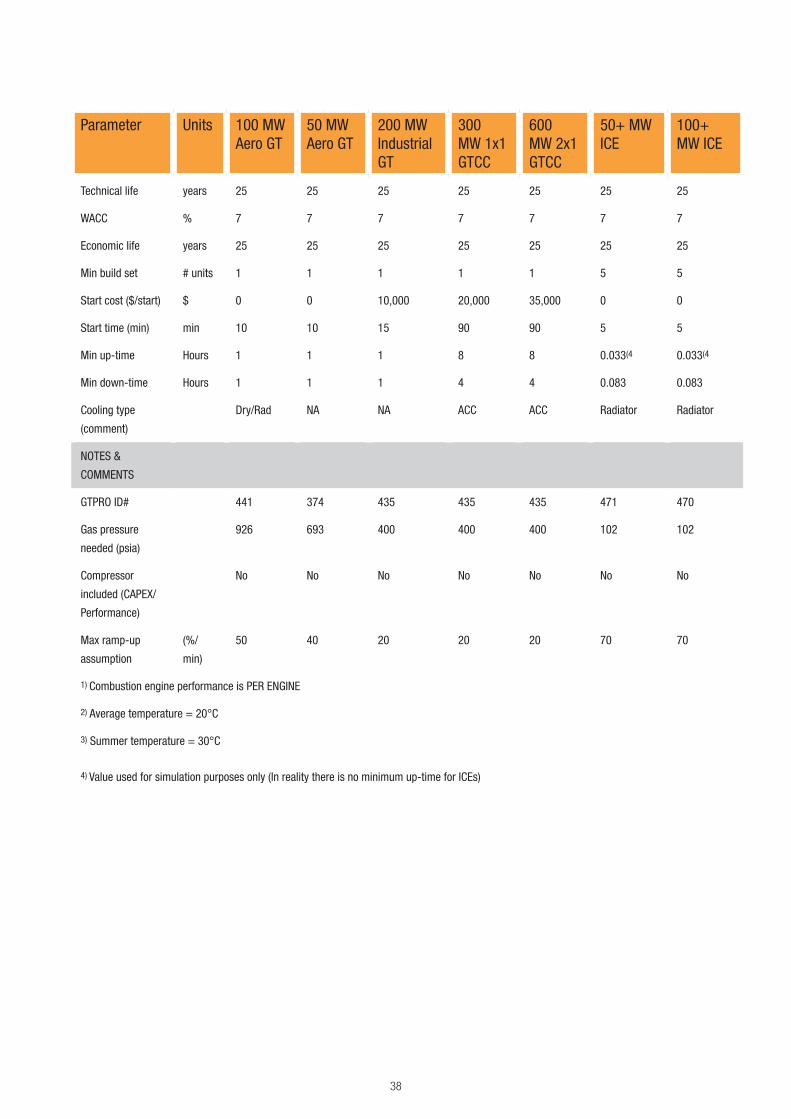
38

Parameter Units 100 MW Aero GT

50 MW Aero GT

200 MW Industrial GT

300 MW 1x1 GTCC

600 MW 2x1 GTCC

50+ MW ICE

100+ MW ICE

Technical life years 25 25 25 25 25 25 25

WACC % 7 7 7 7 7 7 7

Economic life years 25 25 25 25 25 25 25

Min build set # units 1 1 1 1 1 5 5

Start cost ($/start) $ 0 0 10,000 20,000 35,000 0 0

Start time (min) min 10 10 15 90 90 5 5

Min up-time Hours 1 1 1 8 8 0.033(4 0.033(4

Min down-time Hours 1 1 1 4 4 0.083 0.083

Cooling type

(comment)

Dry/Rad NA NA ACC ACC Radiator Radiator

NOTES &

COMMENTS

GTPRO ID# 441 374 435 435 435 471 470

Gas pressure

needed (psia)

926 693 400 400 400 102 102

Compressor

included (CAPEX/

Performance)

No No No No No No No

Max ramp-up

assumption

(%/

min)

50 40 20 20 20 70 70

1) Combustion engine performance is PER ENGINE

2) Average temperature = 20°C

3) Summer temperature = 30°C

4) Value used for simulation purposes only (In reality there is no minimum up-time for ICEs)

WÄRTSILÄ® is a registered trademark. Copyright © 2014 Wärtsilä Corporation.

Wärtsilä Power Plants is a leading global supplier of flexible baseload power plants of up to 600 MW operating on various gaseous and liquid fuels. Our portfolio includes unique solutions for peaking, reserve and load-following power generation, as well as for balancing renewable energy. Wärtsilä Power Plants also provides LNG terminals and distribution systems. As of 2014, Wärtsilä has 56 GW of installed power plant capacity in 169 countries around the world.

www.wartsila.com

Contact: Joseph Ferrari, Wärtsilä Power Plants,

[email protected]

Joseph Ferrari, Market Development Analyst, Wärtsilä Power PlantsMikael Backman, Market Development Director, Wärtsilä Power PlantsJyrki Leino, Senior Power System Analyst, Wärtsilä Power PlantsRisto Paldanius, Business Development Director, Wärtsilä Power PlantsWenxiong Huang, Manager, Technical Consulting, Energy ExemplarNan Zhang, Lead Consultant, Energy ExemplarWenying Hou, Consultant, Energy Exemplar


A WHITE PAPER BY WÄRTSILÄ AND ENERGY EXEMPLAR

POWER SYSTEM OPTIMIZATION BY INCREASED FLEXIBILITYAgile gas-based power plants for affordable, reliable and sustainable power

3

INDEX

Executive summary 4 1. Introduction 52. Modern combustion engine power plants 63. Exploring the impact of combustion engines on system performance 74. Findings 105. Moving forward 16

References 18Appendixes1) Modifications made to the 2022 WECC model 192) Performance parameters for gas engines 20


4

EXECUTIVE SUMMARY:

Great amounts of renewable energy are installed into power systems at state, regional and national level, often due to fulfill legislated mandates or renewable portfolio standards (RPS). While renewable energy is a means for reducing reliance on fossil fuels and decreasing greenhouse gas emissions, it is increasingly evident that there is need for flexible thermal fleet to help balance the renewables. The primary fuel considered for new builds is natural gas, and the default technology to meet capacity and flexibility needs is gas turbines in simple or combined cycle. In this work we show the substantial system benefits of increased flexibility and improved dynamic dispatch capability. This is achieved by exchanging traditional gas turbine based plants in the planning process to gas-fired combustion engine plants. The combustion engine plants have zero start costs and faster start and ramp rates than comparable state-of-the-art gas turbine based plants.

We use the California Independent System Operator (CAISO) as representative of a large system implementing an aggressive 33% RPS by the year 2020. Through simulation of the year 2022, we compare reliability, operational costs, water consumption and CO2 emissions for the CAISO system assuming 5.6 GW of new-build gas turbine-based capacity against a 5.6 GW scenario of combustion engine generation. For modelling, we use PLEXOSTM, a dispatch simulation software by Energy Exemplar.

The rapid start times, superior efficiency and flexibility of gas-fired combustion engines are shown to increase the entire fleet efficiency within the CAISO system, by reducing cycling and starts/stops on existing combined cycles and optimizing provision of ancillary services. Flexibility combined with the superior reliability of multi-shaft engine plants are shown to reduce the number of hours of ancillary service shortfalls by 70%, and the magnitude (MW) of ancillary service shortfalls by more than 50%. The Combustion Engine Alternative scenario shows estimated ratepayer savings of 4–6%, compared to Base Case scenario with gas turbine plants. Water consumption is reduced by 25 million gallons per year, and CO2 emissions are curtailed by 1.1% (> 500,000 short tons per year).


5

Agile gas-based power plants for affordable, reliable and sustainable power

1. INTRODUCTION

Many regions are embarking on aggressive renewable energy mandates, often referred to as Renewable Portfolio Standards (RPS). These are often legislated requirements that by some future year, a certain percentage of a system’s energy consumption (in GWh) be provided by renewable energy, mostly wind and solar. For example, in the USA, 29 states, Washington DC and two US territories have legislated RPS commitments from 10% to 40% by 2015 to 2030 (DSIRE, 2013). The intention is to promote the usage of renewable generation and thereby meet state or regional targets of reduced emissions from the utility sector. The increased usage of variable renewable generation creates new challenges on our utility systems.

There has been surprisingly little exploration into what would happen if the choice of gas-fired generation was expanded and diversified to include other modes of commercially viable, mature technologies suitable for utility-scale power generation. In this work we explore the value of one such technology: medium speed, state-of-the-art combustion engines. As these engines are more flexible than gas turbines with higher response speeds and faster starts, this analysis looks at the system value of increased flexibility and response performance.

We examine installing combustion engine plants instead of gas turbines (GTs) and/or gas turbine combined cycles (GTCCs) for the California Independent System Operator (CAISO) as representative of a large power system with aggressive RPS standards. We address the following issues:

• Thermal fleet CO2 emissions • Water consumption • Operational costs of the system • System reliability • Integrating more renewables We will show that some characteristics of combustion engines make them an attractive alternative to the gas turbine paradigm and can be helpful towards answering in the affirmative to all of these issues.

Definitions

Ancillary services: capacity which the system operator uses to maintain the required balance between generation and load. Also known as balancing services. Divided as contingency and operational reserves. Contingency reserves (spin and non-spin) handle system events, such as a trip of the largest generator. Operational reserves (load following and regulation) are used to balance fluctuations in net load.

Load following: operational reserve to handle discrepancies between the hourly and 5 minute schedules, where schedule differences can arise due to deviations between forecasted and actual renewable output (net load variations).

Net load: the total electricity demand minus renewable generation. This remaining part of the demand has to be met with power generation that can be dispatched, i.e. generating units that can be ramped and/or started and stopped as needed.

Non-spin reserve: off-line capacity available to come on line in the event of a contingency, must satisfy requirements for start-up time and ramping capability

Regulation: operational reserve, balances discrepancies between 5 minute schedule and real time

Spin reserve: online contingency reserve, synchronized to the grid.

6

Modern combustion engine power plants use internal combustion machines that burn natural gas. Unlike GTs, combustion takes place in cylinders, much like a car engine. However, similarity with automotive applications ends there as engines for power plant applications have state-of-the-art control systems and are optimized and developed unlike anything found in the transportation industry. Features of modern combustion engines include:

• Modular (10 to 20 MW per unit) capacity for projects up to 500 MW or more • Highest simple cycle efficiency (46–48% depending on engine model). • Very high part-load efficiency• Insensitive to temperature: no derate on output/efficiency until > 100F/37C• Insensitive to altitude: no derate on output/efficiency until > 5000 ft/1500m• Minimum stable loads of 30% (per engine), as low as 1% for a large multi-engine facility• Engines can ramp from 30% to 100% load in less than 1 minute (ramp rate of 100+%/minute) • Start times of 1–5 minutes, with MWs to grid in 30 seconds.• High reliability and availability• No minimum run time• Minimum down times of 5 minutes• Unrestricted number of starts/stops per day with no impact on O&M (O&M is hours-based only)• Automatic Generation Control (AGC), remote dispatch and black start capability• No process water consumption due to usage of closed loop radiator cooling• Proven technology, power plant applications worldwide, with decades of experience. Wärtsilä, the leading

supplier has over 55 GW of power plant references, 2.7 GW in the USA.

In simple cycle a 300 MW plant with 15 engines (20 MW apiece) can operate at loads as low as the minimum 30% load of one engine, or 6 MW, and with shutting engines down sequentially the plant can be operated over the entire load range (6 MW to 300 MW) at or near full load efficiency by cascading engines on and off.

Combustion engines can also be configured in combined cycle, with approximately 10% more power available from the steam turbine, yielding net efficiencies of 50% or more. This implies that in combined cycle mode, 90% of plant capacity can be online within 5 minutes at over 46% efficiency, and full combined cycle output available in an additional 40 minutes.

Capital costs of combustion engine plants (50 MW to 500 MW) are competitive with modern aeroderivative GTs and combined cycle plants. In terms of emissions, they meet the strictest regulations and have been permitted and installed in states like California, with some of the most stringent emissions requirements in the world.

The leading supplier of combustion engines for power plant applications is Wärtsilä, with over 55 GW of stationary power plant references worldwide. Wärtsilä’s combined cycle offering is trademarked Flexicycle™.

2. MODERN COMBUSTION ENGINE POWER PLANTS

7

3. EXPLORING THE IMPACT OF COMBUSTION ENGINES ON SYSTEM PERFORMANCE

The system (CAISO)

One way to test the impact of increased flexibility on a power system is to simulate the system with a generation fleet with more dynamic capabilities and compare this to the same system using the currently planned resource additions. The system selected for this analysis is the California Independent System Operator (CAISO) in the year 2022. CAISO manages the delivery of electricity to 80% of the state of California and operates the energy and ancillary service markets across three major investor owned utilities. CAISO handles roughly 35% of the electricity load in the western United States.

California has legislative mandates to achieve a 33% RPS by the year 2020. Every two years the California Public Utility Commission (CPUC) issues a Long-Term Planning and Procurement Plan (LTPP) which evaluates capacity needs 10 years into the future. In the 2012 LTPP the CPUC identified approximately 5.63 GW of new-build gas turbine and combined cycle plants by the year 2022. Both the CAISO and the CPUC have recognized that net load fluctuations and ramping will impose considerable integration challenges on their system (CAISO 2014). Thus a test system was available for analysis, whereby the system could be evaluated with the original 5.63 GW of anticipated new-build gas turbines and combined cycles, and then compared to an alternative, where the 5.63 GW was replaced with medium speed combustion engines.

The model (2022 WECC model)

We made use of a publicly available PLEXOS™ database referred to as the 2022 WECC (Western Electricity Coordinating Council) model. PLEXOS™ is a dispatch simulation program that co-optimizes energy and ancillary services, similar to the way in which Security Constrained Economic Dispatch algorithms are used by North American system operators. WECC is the regional reliability entity for the Western Interconnection. The 2022 WECC model includes a basic transmission network among the largest regional entities, and operational information for every power plant in the WECC system. It also includes hourly projections for energy and ancillary services demand and thermal, hydro, wind and solar production. It provides a common framework from which system-wide analyses can be done, as well as state or local level analyses of any subregion of WECC. The 2022 and previous versions of the WECC model have been used by the state of California (CAISO 2011), consultants (e.g. E3 2014a) and by national laboratories (Lew et al. 2013) to explore issues related to renewable integration.

8

Modifications to the model: After consultation with the National Renewable Energy Laboratory (NREL), some modifications were made to better reflect operational capabilities of thermal plants and how they are represented in the model. These modifications are described in Appendix 1. Choice of scenarios for CAISO: The CPUC 2012 LTPP evaluated 4 scenarios. After consultation with analysts from the CPUC we chose to evaluate “Base Case without SONGS”. SONGS is a 2 GW nuclear plant that was ordered to shut down in 2013. The Base Case assumed “mid” growth load forecasts. Details can be found at (CEC, 2012). Fuel costs were built into the model based on the California Energy Commission Burner-Tip pricing forecast 2012–2022.

Ancillary services: Ancillary services (A / S), include operational and contingency reserves and are co-optimized with the energy supply. In the 2022 WECC model they are specified for subregions within WECC region (one of which is the CAISO system). Operational reserves include Regulation (up and down), set to roughly 1.5% of load, as well as Load following. Load following is an operational spinning reserve set aside to handle potential net load fluctuations. Specific to the CAISO system, hourly values (specified in the 2022 WECC model) for load following and regulation are calculated based on a stochastic analysis tool developed by the Pacific Northwest National Laboratory (PNNL) for CAISO. The requirements vary based on load and renewable buildout. Contingency reserves are specified to handle the largest outage in the system, and include Spin Reserve and Non-Spin, at roughly 3% each of load for every hour.

Simulation scope: The day-ahead hourly market was simulated for the entire WECC system for all 8,760 hours in the simulation year 2022. This approach simulates the least-cost dispatch of every plant in the system to serve energy and ancillary services (co-optimized). Results include output (MWh) and production cost (fuel + variable operations & maintenance + start costs + CO2 emissions) of every unit serving energy or ancillary services, as well as the marginal cost for energy and each ancillary service by hour. From these results various metrics can be calculated, such as capacity factor and annual provision (MWh and costs) of energy and ancillary service by asset type (GT, GTCC, ST, etc.). These and other results were extracted for the CAISO system from the 2022 WECC simulation results. Import and export of energy from the CAISO system were accounted for across interties with neighboring regions.

Two types of simulations were performed:

Need runs: Full production cost model but with the maximum Load following up and Regulation up requirement for the month assigned to each hour, and with certain costs relaxed (such as start costs). Purpose is to apply a “worst case” ancillary service requirement scenario and thereby identify any potential capacity shortfalls independent of the economics associated with dispatchable generation.

Production cost runs: Full production cost run with prescribed daily/hourly values for energy and A/S, and with all costs enabled. Purpose is to estimate CO2, variable cost of annual fleet operation and to identify any potential shortfalls in generation or ancillary services.

9

The Base Case and the Combustion Engine Alternative

Two separate cases were defined. The Base Case assumes all new-builds (between 2012 and 2022) are exactly as specified by the California Public Utility Commissions 2012 LTPP: 5.63 GW of gas turbines in simple and combined cycle. The Combustion Engine Alternative performs the same simulation with the same assumptions and inputs, except instead of the 2012 LTPP gas turbine new-builds, an equivalent capacity of 5.63 GW of combustion engines in simple and combined cycle were assumed to be built instead.

Base Case: Defined as including the GT based new-builds (simple and combined cycle) in the 2012 LTPP, expected to be online by the simulation year 2022.

• 760 MW of industrial GTs• 1,992 MW of aeroderivative GTs• 2,875 MW of GT combined cycles

All parameters for these units were maintained exactly as specified in the 2022 WECC model.

Combustion Engine Alternative: Defined as removal of all new-build GTs and GTCCs from the Base Case and replacement by 2,752 MW of combustion engines with operational characteristics similar to the Wärtsilä 18V50SG engine. The value of 2,752 MW is the sum of industrial and aeroderivative GT capacity defined in the Base Case, so it is a direct substitution of simple cycle combustion engines for simple cycle GTs. In addition, 2,875 MW of combustion engines in combined cycle substitute for the new-build GTCCs. These are equivalent to Wärtsilä Flexicycle™ plants. Details of the units and operational characteristics (start times, VOM rates, start costs, full load output and efficiency on a per-plant basis) can be found in Appendix 2.

10

Figure 1. Shortfall by ancillary service type Base Case and Combustion Engine Alternative.

Combustion engines reduce capacity shortfalls for ancillary services

The first set of simulations was the “Need Runs”, which determined if enough capacity exists to meet system needs. Shortfalls were only observed for the peak day, 7/22/2022. For the Base Case (GT buildout) there were a total of 6 hours of shortage with a maximum shortfall of 2.71 GW, compared to the Combustion Engine Alternative with 2 hours of shortage with a maximum shortfall of 1.37 GW (Figure 1).

4. FINDINGS

3 000

2 500

2 000

1 500

1 000

500

0

Hour

1 2 3 4 5 6 7 8 9 10 11 12 13 14 15 16 17 18 19 20 21 22 23 24

NonSpin

LF_Up

MW

3 000

2 500

2 000

1 500

1 000

500

0

Hour

1 2 3 4 5 6 7 8 9 10 11 12 13 14 15 16 17 18 19 20 21 22 23 24

NonSpin

LF_Up

MW

Combustion Engine Alternative

Base Case

11

Combustion engines reduce CO2 emissions by 1.1%

Medium speed combustion engines in simple cycle require approximately 8-10% less fuel per MWh than the most efficient gas turbines on the market, and hence emit at least 8-10% less CO2/MWh. The efficiency advantage of combustion engines becomes even greater at part-loads. Combustion engine combined cycles, in contrast, use about 10% more fuel (and emit about 10% more CO2) than modern, advanced GTCCs at full load. However, 90% of a combustion engine combined cycle’s output is available within 5-7 minutes at a heat rate of 8,400 to 8,500 Btu/kWh (@ 46% net, LHV efficiency), with full combined cycle output and efficiency in 45 minutes from start command. In contrast, gas turbine combined cycles get roughly 2/3 of their capacity within 15 minutes of the start command, at a heat rate of 10,800 Btu/kWh (@ 35% net, LHV efficiency) and up to 1 or more hours before full load output and efficiency. In short, per start sequence, the combustion engine combined cycle emits less CO2.

So the question is, does the capacity replacement in the Combustion Engine Alternative ultimately increase or reduce the CO2 emissions from the CAISO fleet? The efficiency of the thermal fleet in the Base Case was 0.7% lower (7,444 Btu/kWh) than that of the fleet in the Combustion Engine Alternative (7,390 Btu/kWh). This was influenced in large part by the higher efficiency of the Wärtsilä units and by the increased capacity factor at higher efficiency for the combined cycle fleet (52.89% cf at 7,168 Btu/kWh in Combustion Engine Alternative relative to 49.86% cf at 7,215 Btu/kWh in the Base scenario). In addition, existing combined cycles in the Combustion Engine Alternative started 20% fewer times per year (on average) than in the Base Case. Taking the enhanced fleet efficiency and reduced number of GTCC starts into account, the Combustion Engine Alternative delivered a CO2 reduction for the CAISO thermal fleet of 1.1%, which equates to more than 500,000 short tons/year. In brief, this system optimization is realized not just by having a more efficient simple cycle fleet but through a better utilization of the combined cycle assets once the dynamic, variable portion of their dispatch has been taken over by more flexible assets, in this case combustion engines.

Combustion engines reduce water consumption

Given the concern over water rights and availability in the western United States as a whole, and in California in particular, it can be assumed that any new combined cycles installed by year 2022 will minimize water consumption by using air-cooled condensers, or ACC’s (instead of cooling towers). The combustion engine combined cycles (Flexicyle™) were assumed to use ACC’s as well. Each of these combined cycle configurations still has a water concern related to boiler makeup.

Combustion engine combined cycles use 1/3rd the water of a GTCC: Detailed calculations for boiler makeup water flow rates are quite dependent on water chemistry, the equipment involved, the types of water treatments used, unit cycling characteristics etc. In lieu of detailed calculations, we can take a heuristic approach. Approximately 30% of a GTCC’s output is from the steam turbine. A similar sized combustion engine combined cycle would get approximately 10% of its power from the steam turbine. Without detailed calculation, it would be safe to say that a combustion engine combined cycle would use only one-third of the water for boiler makeup of that required from a GTCC per MWh. This is a conservative estimate as combustion engine combined cycles use low pressure boilers, so attendance to water chemistry (and the need for makeup) are reduced relative to the larger, superheated boilers used in GTCCs.

Combustion engines could save more than 25 million gallons of water per year: The 2012 LTPP highlighted 1,550 MW of 100 MW/unit class aeroderivative units which often use water injection, and are representative of some of the most advanced gas turbines available. Power and efficiency are augmented by two means, an intercooler and water injection. The intercooler reduces the temperature of air flowing into the combustor, thereby increasing its density, which allows for more power extraction per unit of fuel consumed. Water injection is then added to increase mass flows through the rotors and increase power production.

12

Assuming the 100 MW class turbines noted in the 2012 LTPP are offered with water injection and dry coolers (radiators) for intercooler heat rejection, the database GTPRO V23 (www.thermoflow.com) estimates water injection rates at approximately 24.53 gallons/MWh (or 0.1 m3/MWh). The four plants across which the 1,550 MW were added generated, in the Base Case production cost run, 1,041,346 MWh for the year 2022. This equates to 25,544,224 gallons (97,000 m3) of water consumed for water injection. In the Combustion Engine Alternative, these units were replaced with Wärtsilä 18V50SG capacity, which is also air cooled but requires no water for injection.

Combustion engines optimize ancillary service provision

Combustion Engines in multi-unit plants have much higher plant reliability (on a per 100 MW basis) than gas turbine alternatives. In addition, combustion engines have faster ramp rates and shorter start times. Taken together, this implies that in a supply/demand context, an equivalent amount of combustion engine capacity will provide a greater supply of available ramping capacity, primarily for upward ancillary services – and, consequently, a reduced marginal cost of provision of those ancillary services. These units maintain a very high efficiency across the load spectrum, from minimum output (Pmin) to maximum output (Pmax).

In the Combustion Engine Alternative, combustion engines provided greater amounts of Load following up (LFUP), Regulation up (RegUp), and Spin and Non-spin reserves, than the units they supplanted in the Base Case (Figure 2.-5.). In addition, adding 5.63 GW of combustion engine capacity in lieu of the LTPP GT-based buildout, reduced the provision of LFUP, RegUp and Spin reserve by existing GTs and GTCCs. In particular, the existing fleet of GTCCs, in the Combustion Engine Alternative, are tasked less with part-load operations at reduced efficiency to provide uplift ancillary services. This allows them to run more hours at or near full load and their maximum efficiency (see efficiency gain discussion in prior section on CO2 reductions).

13

6000

5000

4000

3000

2000

1000

0GTCC New

Base (New Build GT/GTCC)

Combustion engine Alternative

Annu

al M

Wh

prov

isio

n

Wärtsilä Flexicycle™

GT (New) Wärtsilä50SG

Existing GTCC

Existing GT

Figure 2. Provision of Load Following Up (LFUP) ancillary service for the two scenarios. Combustion engines provide 30% more LFUP than the gas turbine/Base buildout, and reduce provision of LFUP by the existing GTs and GTCCs.

1200

1000

800

600

400

200

0GTCC New



Annu

al M

Wh

prov

isio

n



Existing GTCC

Existing GT

4500

4000

3500

3000

2500

2000

1500

1000

500

0

GTCC New

Annu

al M

Wh

prov

isio

n



Existing GTCC

Existing GT



Figure 5. Provision of Non-Spin ancillary service for the two scenarios. Due to fast start up times and high reliability, combustion engines provide 50% more Non-Spin than the gas turbine/Base buildout and reduce provision of Non-Spin by the existing GTs by 50%.

3500

3000

2500

2000

1500

1000

500

0GTCC New

Annu

al M

Wh

prov

isio

n



Existing GTCC

Existing GT



Figure 3. Provision of Regulation Up (RegUp) ancillary service for the two scenarios. Combustion engines provide more than double the amount of RegUp compared to the gas turbine/Base buildout and reduce provision of this A/S by the existing GTs and GTCCs.

Figure 4. Provision of Spinning Reserve (Spin) ancillary service for the two scenarios. Simple cycle combustion engines provide double the amount Spin compared to the GTs in the Base scenario.

14

Combustion engines reduce wholesale generation costs by up to 6% per year

Wholesale generation costs were calculated as follows for each hour based on full PLEXOS™ production cost runs:

1) Energy cost as the MWh (generated) times the marginal price. a. Marginal price is the $/MWh (Fuel + VOM + Emissions) for the last generator added to the dispatch stack in the model, which is reflective of the marginal unit.

2) Ancillary service cost (by type) as the MWh required to fulfill A/S requirements times the shadow price of each A/S. a. A/S type included regulation up/down, load following up/down, spin reserve, nonspin reserve. b. Shadow price is the incremental cost ($/MW) to provide one additional MW of that service, reflective of the marginal cost (by type).

3) Shortfall cost as the MWh shortfall times a value of lost load (VOLL) cost for shortage (of energy or A/S by type) a. The VOLL estimate (simple form) applies a shortage cost of $15,000/MWh (NARUC, 2013). b. The VOLL estimate (less simple) applies a premium to shortage on uplift AS, specifically $50,000/MWh for load following up (E3, 2014).

Quantification of shortages: Shortages were only observed on the peak day (Table 1).

Quantification of wholesale level savings: The sum of items 1, 2 and 3 above were calculated as conservative proxies of savings. The calculated values were considered conservative as the marginal costs are based solely on production cost of the marginal unit and do not include any markups related to stakeholder bidding strategies.

Table 1. Ancillary service shortages on peak day for both the Base Case and Combustion Engine Alternative

Peak day (7/22/2022) A/S shortages (MWh) Base Combustion Engine

Alternative Delta% Reduction with


Load following up 4,648 1,157 3,491 75%

Non-spin 1,505 0 1,505 100%

15

Table 2. Estimated ratepayer savings with Combustion Engine Alternative under 3 assumptions for shortfall costs for ancillary services.

Annual costs ($ ,000) Base Combustion Engine Alternative Delta

% Reduction with Combustion Engine

Alternative

Energy cost 9,000 8670 330 4%

Non-shortage A/S cost 204 165 39 19%

Totals (no cost for shortfalls) 9,204 8,835 369 4%

Shortage A/S Cost ($15k/MWh) 92.3 17.4 74.9 81%

Totals (w/$15k/MWh for shortfalls) 9,296 8,852 444 5%

Shortage AS Cost ($50k/MWh for LFUP) 255 58 197 77%

Total (w/LF Up shortfall at $50k/MWh) 9,459 8,893 566 6%

16

The results of this analysis demonstrate that a diversified generation portfolio, one that includes combustion engine technology, can assist large power systems with renewable integration while simultaneously reducing CO2 emissions and water consumption and reducing costs ultimately borne by ratepayers. For example, in this study simply changing a modest portion of the thermal fleet can improve operational profiles and capacity factors for combined cycles, and improve overall system efficiency. It should be noted that the purpose of this analysis was not to find the theoretically optimal mix of the different gas fired generation technologies for a future California system but rather to show one example of savings based on exchanging the new-build out from gas turbine based plants to combustion engine based plants. The benefits at the fleet level have been demonstrated for the CAISO system in a prior study (Kema 2013) as well as for the United Kingdom (Wärtsilä, Redpoint Energy 2013). The findings of this study and the others mentioned give rise to additional issues related to the benefits combustion engines bring to power systems.

Capital costs of combustion engines are competitive with gas turbine solutions (E3, 2014a). Their competitiveness in regards to providing affordable flexibility is increasingly recognized by international agencies. For example, the International Energy Agency reports that, with regards to provision of flexibility, the levelized cost of combustion engines is competitive with advanced combined cycles (IEA 2014).

System reliability can be increased with modular buildout of capacity in 10-20 MW increments. The unscheduled outage rate for a 20 MW Wärtsilä engine is on the order of 1%. For a five engine, 100 MW plant the probability that all engines will experience unscheduled outages at the same time is 0.01^10, or 10-8 %. Therefore the likelihood of system reliability impacts from outages per 100 MW of capacity is reduced relative to alternate capacity options that can only be offered in 100, 200, 300 MW or larger blocks.

Similar to findings by PNNL (Makarov et al. 2008) related to time response characteristics of energy storage, there is reason to expect that modular, fast start, high ramp rate combustion engine plants can meet the flexibility needs of power systems with less installed capacity. This is indirectly attested to in this study by the fact that with matching new-build capacity installed, there was a dramatic reduction in shortfall hours and magnitudes for ancillary services in the Combustion Engine Alternative scenario (Figure 1 and Table 1).

Can a diversified fleet help systems absorb greater amounts of renewable energy than a less diverse fleet? Yes. Multi-unit combustion engine plants can start in <5 minutes to full load, provide MW to the grid in 30s from the start command, and operate at very low minimum loads. This aspect alone would be of great value for power systems such as CAISO which expect to experience massive net load ramps in shoulder months as they approach their 33% RPS in 2020.

5. MOVING FORWARD

17

As solar and wind energy peak, the standard assumption is that combined cycle assets will cycle and/or be idled back to low loads (e.g. ISO-NE 2010; Lew et al. 2013). This is done so that when wind/solar production declines, the needed ramp capacity is available to meet the net load increase/ramp. Instead of idling large combined cycles at low loads, with commensurate increases in CO2 production (by MWh) as their efficiencies are compromised, a capacity bank of offline combustion engine resources could meet net load ramps from an idle state. This would alleviate a potential problem highlighted in a recent report (E3, 2014b). In that report, it was noted that as RPS standards for California approach 40% or higher, there is a “lower net load bound” that limits the amount of renewable energy the system can utilize, especially during peak solar production hours. A certain amount of thermal generation must be kept online in a part-loaded state to meet the expected net load ramps as wind/solar production decline in the afternoon/evening. This, in turn, means that there is an upper bound to the amount of renewable energy the system can absorb. Banks of combustion engines can provide that needed ramp capacity from an unloaded state, which would reduce the lowest net load the thermal fleet could support, which in turn would allow for greater utilization of renewable GWh. In other words, the system could integrate larger amounts of renewable energy by using less thermal generation if that generation had more flexibility. In addition, this would further reduce CO2 emissions on an annual basis. The full potential of a diversified thermal fleet in terms of helping nations, states, ISOs/RTOs maximize renewable generation while minimizing CO2 production is, at least in part, impacted by market rules in effect. In many cases these rules were created decades ago based on the capabilities of generation at that time and with no foresight into the emergence of renewable generation. In order to fully exploit the capabilities of a diversified portfolio (including combustion engines storage technologies and demand response) it is necessary for market designers to recognize the capabilities of today’s technology. In this work we have shown the value of a diverse portfolio that includes medium speed combustion engines, based on current market rules in the context of the system modeled (CAISO). We hope this will stimulate further discussion on the broader issue of market design required to unlock the full potential of a diversified portfolio.

18

CAISO (2013a) Fast Facts: What the Duck Curve Tells Us About Managing a Green Grid. http://www.caiso.com/Documents/FlexibleResourcesHelpRenewables_FastFacts.pdf

CAISO (2013b) Summary of Preliminary Results of 33% Renewable Integration Study – 2010 CPUC LTPP Docket No. R.10-05-006. http://www.cpuc.ca.gov/NR/rdonlyres/E2FBD08E-727B-4E84-BD98-7561A5D45743/0/LTPP_33pct_initial_results_042911_final.pdf

CAISO (2014) Flexible Resource Adequacy Criteria and Must-Offer Obligation, Draft Final Proposal, Feb 7, 2014. https://www.caiso.com/Documents/DraftFinalProposal-FlexibleResourceAdequacyCriteriaMustOfferObligation.pdf

CEC (2012) California Energy Commission Mid-Case Revised Demand Forecast Forms. http://www.energy.ca.gov/2012_energypolicy/documents/2012-02-23_workshop/mid_case/

DSIRE (2013) Database of State Incentives for Renewables & Efficiency. http://www.dsireusa.org/documents/summarymaps/RPS_map.pdf

E3 (Energy+Environmental Economics) (2014a) Capital Cost Review of Power Generation Technologies, Recommendations for WECC’s 10- and 20- year studies. Report prepared by E3 for the Western Electric Coordinating Council, March 2014.

E3 (Energy+Environmental Economics) (2014b) Investigating a Higher Renewables Portfolio Standard in California. http://www.ethree.com/documents/E3_Final_RPS_Report_2014_01_06_with_appendices.pdf

IEA (2014). The Power of Transformation - Wind, Sun and the Economics of Flexible Power Systems, 238 pages. International Energy Agency. http://www.iea.org/w/bookshop/add.aspx?id=465

ISO-NE (2010) Final Report: New England Wind Integration Study. http://www.iso-ne.com/committees/comm_wkgrps/prtcpnts_comm/pac/reports/2010/newis_report.pdf

Kema (2013) How to Manage Future Grid Dynamics: Quantifying Smart Power Generation Benefits. Prepared by KEMA, Inc, 2/14/2013. http://www.smartpowergeneration.com/spg/files/library/Smart_Power_Generation_Benefits_final_rev_2-14.pdf

Lew D, G Brinkman, E Ibanez, A Florita, et al, (2013) National Renewable Energy Laboratory, Western Wind and Solar Integration Study, Phase 2. http://www.nrel.gov/docs/fy13osti/55588.pdf

Makarov, YV, J Ma, S Lu, TB Nguyen (2008) Assessing the Value of Regulation Resources Based on Their Time Response Characteristics. Pacific Northwest National

Laboratories. http://www.pnl.gov/main/publications/external/technical_reports/PNNL-17632.pdf

NARUC (2013) The Economic Ramifications of Resource Adequacy White Paper, Astrape Consulting, January 2013.http://www.naruc.org/grants/Documents/Economics%20of%20Resource%20Adequacy%20WhitePaper_Astrape_Final.pdf

Wärtsilä, Redpoint Energy (2013). Flexible energy for efficiency and cost effective integration of renewables in power systems. A Wärtsilä white paper supported by modelling conducted by Redpoint Energy, a business of Baringa Partners. http://www.smartpowergeneration.com/spg/files/library/Flexible-energy-for-integrationof-renewables_Wartsila_2013.pdf

REFERENCES

19

The following modifications were made to the 2022 WECC model

Part-load heat rates: In the 2022 WECC model a number of generating plants were assigned a single-point, full load heat rate. The PLEXOS™ software interprets this as the plant being capable of operating between its minimum and maximum loads (Pmin and Pmax) while maintaining full load heat rate. This is technically and physically not possible, and could result in ancillary service allocations for those specific facilities. This would require them to operate at loads below Pmax, based on variable costs erroneously calculated based on full load heat rate. Therefore we identified over 900 thermal plants in the WECC model with single point heat rates, and provided the PLEXOSTM model with assumed part-load heat rate profiles for these plants. These assumed part-load heat rate profiles were created for aeroderivative and industrial gas turbines, combined cycles and boiler/steam turbine plants, using output from the commercially available software GTPRO V23 (www.thermoflow.com). The part-load heat rates for each individual plant were then scaled from the full load heat rate in the model using the supplied profiles.

Max replacement parameter: Any plants within or associated with the state of California that had max replacement parameters had this parameter removed. In essence, the presence of this parameter implies a unit can supply full or part-load within 10 minutes from an idle state. This is incorrect when applied to combined cycles and steam turbines which may have start times in excess of 3 hours. A total of 1,039 MW of capacity was modified.

Start profiles: All combined cycles with no assigned start profiles were assigned WECC average start profiles (a total of 145 GTCCs).

APPENDIX 1. MODIFICATIONS MADE TO THE 2022 WECC MODEL

20

Combustion engines engine plants were assumed to replace the following facilities in the 2022 WECC Model

APPENDIX 2. PERFORMANCE PARAMETERS FOR COMBUSTION ENGINES

Base CaseRESOURCE ADDITIONS (on line by 2022)

Plant

Mariposa EC CT1, CT2, CT3, CT4

Sentinel_1 to Sentinel_8

Walnut Crk_1 to Walnut Crk_5

Escondido CT

SCE LCR*

SDGE LCR*

Marsh Landing CT1, CT2, CT3, CT4

El Segundo 2_5 & El Segundo 2_7

Lodi Energy Ctr

PalmdaleHybrid

Russell City Energy Ctr

SCE LCR*

Total

Capacity (MW)

200

850

500

45

100

297

760

550

255

570

600

900

5627

GT Configuration

Aero

Aero

Aero

Aero

Aero

Aero

Industrial

GTCC

GTCC

GTCC

GTCC

GTCC


# of gas engines

10

43

25

2

5

15

38

26

12

27

28

42

Type

Simple Cycle

Simple Cycle

Simple Cycle

Simple Cycle

Simple Cycle

Simple Cycle

Simple Cycle

Combined Cycle

Combined Cycle

Combined Cycle

Combined Cycle

Combined Cycle

Capacity (MW)

200

860

500

40

100

300

760

559

258

580.5

602

903

5663

Table 3. Base Case gas turbine capacity and Combustion Engine Alternatives

* LCR = Local Capacity Resource Addition

21

Parameter Unit 20 MW medium speed combustion engine*

20 MW medium speed combustion engine

in combined cycle **

Max Capacity MW 20.00 21.5

Min Stable Level MW 6.00 6.45

Load Point (30%) MW 6.00 6.45

Load Point (50%) MW 10.00 10.75

Load Point (75%) MW 15.00 16.13

Load Point (Full Load) MW 20.00 21.50

Heat Rate (30%) Btu/kWh 10,501 9,404

Heat Rate (50%) Btu/kWh 9,221 8,345

Heat Rate (75%) Btu/kWh 8,711 7,993

Heat Rate (Full Load) Btu/kWh 8,291 7,763

Max Ramp Up MW/min 14.00 15.05

Max Ramp Down MW/min 21.00 22.58

Run Down Rate MW/min 18.00 19.35

Min Up Time hours 0.03 0.03

Min Down Time hours 0.08 0.08

Start cost USD 0 0

VOM cost USD/MWh 3.5 3.5

* Performance based on a Wärtsilä 18V50SG engine** Performance based on a Wärtsilä Flexicycle™ (18V50SG engine in combined cycle)

Table 4. Combustion engine performance on a per-unit basis. Plant sizes 500+MW obtained by arranging multiple units in parallel.

22

WÄRTSILÄ® is a registered trademark. Copyright © 2014 Wärtsilä Corporation.

Wärtsilä Power Plants is a leading global supplier of flexible baseload power plants of up to 600 MW operating on various gaseous and liquid fuels. Our portfolio includes unique solutions for peaking, reserve and load-following power generation, as well as for balancing renewable energy. Wärtsilä Power Plants also provides LNG terminals and distribution systems. As of 2014, Wärtsilä has 56 GW of installed power plant capacity in 169 countries around the world.

www.wartsila.com

Contact: Joseph Ferrari, Wärtsilä Power Plants, [email protected]

Joseph Ferrari, Market Development Analyst, Wärtsilä Power PlantsMikael Backman, Market Development Director, Wärtsilä Power PlantsJyrki Leino, Senior Power System Analyst, Wärtsilä Power PlantsRisto Paldanius, Business Development Director, Wärtsilä Power PlantsWenxiong Huang, Manager, Technical Consulting, Energy ExemplarWenying Hou, Consultant, Energy Exemplar
