NBER WORKING PAPER SERIES

WAR, SOCIALISM AND THE RISE OF FASCISM:AN EMPIRICAL EXPLORATION

Daron AcemogluGiuseppe De FeoGiacomo De Luca

Gianluca Russo

Working Paper 27854http://www.nber.org/papers/w27854

NATIONAL BUREAU OF ECONOMIC RESEARCH1050 Massachusetts Avenue

Cambridge, MA 02138September 2020

We thank Luigi Pascali, Giacomo Ponzetto, Riccardo Puglisi, Guido Tabellini, Joachim Voth and the participants to the CEPR Political Economy Webinar for useful comments and suggestions. We would also like to thank Amos Conti, Annagrazia De Luca, Stefano Presti and Raffaele Savarese for the assistance provided in data collection and digitization and gratefully acknowledge the financial support of the Morrell Trust and the extensive support received by the employees of the many state archives and libraries visited around the country, in particular the director of the National Central Library of Florence, Luca Bellingeri, and Gian Luca Corradi, Enrico Leonessi, Annalisa Moschetti, Annalisa Pecchioli and Lina Tavernelli. This paper combines two independent working papers, “War, Socialism and the Rise of Fascism: An Empirical Exploration” by Acemoglu, De Feo and De Luca and “World War One and the Rise of Fascism in Italy" by Russo. The views expressed herein are those of the authors and do not necessarily reflect the views of the National Bureau of Economic Research.

NBER working papers are circulated for discussion and comment purposes. They have not been peer-reviewed or been subject to the review by the NBER Board of Directors that accompanies official NBER publications.

© 2020 by Daron Acemoglu, Giuseppe De Feo, Giacomo De Luca, and Gianluca Russo. All rights reserved. Short sections of text, not to exceed two paragraphs, may be quoted without explicit permission provided that full credit, including © notice, is given to the source.

War, Socialism and the Rise of Fascism: An Empirical ExplorationDaron Acemoglu, Giuseppe De Feo, Giacomo De Luca, and Gianluca RussoNBER Working Paper No. 27854September 2020JEL No. D72

ABSTRACT

The recent ascent of right-wing populist movements in many countries has rekindled interest in understanding the causes of the rise of Fascism in inter-war years. In this paper, we argue that there was a strong link between the surge of support for the Socialist Party after World War I (WWI) and the subsequent emergence of Fascism in Italy. We first develop a source of variation in Socialist support across Italian municipalities in the 1919 election based on war casualties from the area. We show that these casualties are unrelated to a battery of political, economic and social variables before the war and had a major impact on Socialist support (partly because the Socialists were the main anti-war political movement). Our main result is that this boost to Socialist support (that is “exogenous” to the prior political leaning of the municipality) led to greater local Fascist activity as measured by local party branches and Fascist political violence (squadrismo), and to significantly larger vote share of the Fascist Party in the 1924 election. We document that the increase in the vote share of the Fascist Party was not at the expense of the Socialist Party and instead came from right-wing parties, thus supporting our interpretation that center-right and right-wing voters coalesced around the Fascist Party because of the “red scare”. We also show that the veterans did not consistently support the Fascist Party and there is no evidence for greater nationalist sentiment in areas with more casualties. We provide evidence that landowner associations and greater presence of local elites played an important role in the rise of Fascism. Finally, we find greater likelihood of Jewish deportations in 1943-45 and lower vote share for Christian Democrats after World War II in areas with greater early Fascist activity.

Daron AcemogluDepartment of EconomicsMIT50 Memorial DriveCambridge, MA 02142-1347and NBERdaron@mit.edu

Giuseppe De FeoUniversity of LeicesterSchool of BusinessBrookfield Campus266 London RoadLeicester LE2 1RQUnited Kingdomgdf9@leicester.ac.uk

Giacomo De LucaFree University of Bozen giacomo.deluca@york.ac.uk

Gianluca RussoBoston University270 Bay State RdBoston, MA 02215 russog@bu.edu

1 Introduction

As we approach the centennial of the March on Rome in 1922, which catapulted Benito Mussolini’s fascists

to power in Italy, there is renewed interest in fascism, partly as a result of the rise of right-wing authoritarian

populist movements around the world (e.g., Stanley, 2018). There is, however, little agreement on what led

to the rise of fascist politics in interwar Europe in the first place. Prominent theories range from cultural

ones (e.g., Sternhell et al., 1994) to social psychological ones (e.g., Lasswell, 1933; Fromm, 1941; Adorno

et al., 1950; Laclau, 1977), to sociological ones (e.g., Ortega Y Gasset, 1932; Parsons, 1942; Lipset, 1955)

and to historical approaches such as those of Moore (1966), Griffin (1991) and Kershaw (2015). One of

the most enduring areas of disagreement has been the relationship between socialism and fascism. The

German historian Ernst Nolte (1965), as well as several Marxist historians, have emphasized that fascism,

and the support it received from both the upper and middle classes, was related to the threat of socialism in

the immediate aftermath of WWI (see for example Snowden, 1972; Corner, 1975; Demers, 1979; Cardoza,

1982; Lyttelton, 2003). Yet several other historians have disagreed with this interpretation (e.g., Griffin,

1991; Sternhell et al., 1994). This debate is not just academic. If Fascism was unique to a period in which

World War I and the Soviet revolution had created a threat of socialist revolution in continental Europe,

then there may be less reason to fear that today’s right-wing authoritarian and populist movements will turn

fascist.

In this paper, we contribute to this debate by providing evidence that the (perceived) threat of socialism

was critical to the rise of fascist politics in Italy. The Italian Socialist Party was one of the strongest in

Europe in the first quarter of the 20th century and was committed to the hard-line socialist/communist

agenda (Tasca, 1938). After the 1917 Bolshevik revolution, it allied itself with the Soviet Russia. Because

it had opposed Italy’s entry into World War I, the hardship suffered by Italians who served in the war and

those who remained behind created a groundswell of support for the party, which captured 32.3% of the

national vote in the 1919 elections (Maier, 1988, p. 129). At this point, the Fascist Party lacked a coherent

program and did not even manage to compete effectively in the election. Subsequently, however, the Fascists

started receiving support from many local elites and middle-class Italians alarmed by the socialist threat (De

Felice, 1965). By 1920, the Fascists were better organized, received monetary and political backing from

many anti-socialist landowners and businessmen, and had started carrying out systematic violence against

Socialists and other politicians and organizations that opposed them. By 1924, a significant fraction of the

right-wing and center-right vote shifted to the Fascist Party, which received more than 65% of the vote in the

parliamentary elections (Direzione Generale della Statistica, 1924). In the words of Tasca (1938, p. XVI),

“On November 16, 1919, in the first general election since the war, Mussolini obtained only

5000 votes in Milan [...]. The socialist paper Avanti announced ironically that a corpse had been

fished up from the bottom of the Naviglio canal in an advanced state of decay — Mussolini’s.

2

A year and half later the ‘corpse’ [...] was elected at the head of the candidates of the national

bloc in two constituencies, Milan and Bologna. After the beginning of 1922 the fascist advance

became an avalanche, and Mussolini left Milan in a sleeping-car on the evening of October

29 to ‘march’ on Rome, where he had been invited by the king to form a cabinet. This rapid

success, which on the face of it seems little short of miraculous, was the result of a combination

of factors, [...] and above all from the world war and its repercussions.”

Our empirical strategy is to investigate the linkage between the threat of socialism and the rise of fas-

cist politics in Italy. We first substantiate the aforementioned claim that the war’s hardship created a big

boost to the Socialist Party in the 1919 election. We use the military Roll of Honor to obtain estimates of

Italian casualties by municipality during WWI. We document that the casualties of footsoldiers in a mu-

nicipality were unrelated to any prior political, economic, social or demographic aspects of municipalities.

Nevertheless, we show that municipalities with high casualties (and thus with greater exposure to the war)

experienced a sizable increase in the vote share of the Socialist Party in the 1919 elections (relative to the

1913 elections). We interpret the WWI casualties as an exogenous source of variation in Socialist support

and trace the subsequent political responses to this variation.

Our main finding is that in municipalities experiencing this boost to Socialist support saw a powerful

Fascist response. In particular, we estimate greater likelihood of local Fascist branches and more Fascist

violence in the 1920s, and significantly higher Fascist vote share in the 1924 elections in these areas. Our

estimates suggest that as much as 15% of the increase in the vote share of the Fascist lists from 1919 to 1924

may have been due to to the consolidation of the right-wing and center-right vote under the auspices of this

party in the face of the perceived red scare.

We bolster this interpretation with several exercises. First, we show that the source of variation we

exploit is unlikely to be confounded by other, competing explanations. For example, we do not find a

consistent support from veterans for the Fascist Party, and our instrument does not predict the building of

nationalist (war) memorials. Second, we demonstrate that the increase in the vote share of the Fascist Party

was not at the expense of the Socialist Party. Third, we document that the shift towards the Fascist Party was

stronger when the threat of socialism coincided with a larger fraction of elites and urban middle classes, and

provide additional evidence that this is both because some of the elites supported the Fascist Party and the

local “petty bourgeoisie” switched its allegiance from center-right parties to the Fascists.

Furthermore, if the rise of Fascism was partly a response to the threat of socialism, then other shocks

intensifying Socialist support should have similar effects. We document that this is the case, exploiting

rainfall variation, leading to drought in some municipalities, and the differential effects of the Spanish flu

epidemic across municipalities. In both cases the results are not as precise as our main estimates, but are

consistent with a causal channel working from hardship to support for the Socialist Party and from there to

subsequent rise of the Fascist Party in the early 1920s.

3

Finally, we explore two longer-term effects of Fascism. First, we show that support for Fascism is asso-

ciated with greater likelihood of Jews being deported from the area during 1943-45, presumably reflecting

local collaboration with the Nazis. Second, we document that in the post-Fascist era elections, in munici-

palities where the Fascist Party was more successful, center-right parties performed significantly worse and

center-left and other left-wing parties performed better. This may have been because their alliance with the

Fascists in the 1920s may have partly delegitimized center-right establishment.

In addition to the historical literature discussed previously, our paper is related to a few works in political

economy. A recent strand of literature analyzes the roots of the Nazi movement in Germany. Voigtländer

and Voth (2012) document the links between anti-Semitic pogroms in the Middle Ages and support for the

Nazi Party, while Satyanath et al. (2017) demonstrate the role of local associations. Adena et al. (2015) and

Voigtländer and Voth (2019) explore the effects of radio propaganda and public works, such as the building

of the Autobahn network, on Nazi support. Recent work by Koening (2015) investigates the link between

returning war veterans and support for right-wing parties in Germany.1 Even more closely related to our

work are a few papers that show the effects of economic disruption and hardship on later Nazi support. In

particular, Galofré-Vilà et al. (2017) and King et al. (2008) focus on the effects of the Great Depression,

while Doerr et al. (2020) explore the consequences of the 1931 banking crisis.

There are fewer econometric studies of the rise of Italian Fascism, though there is a sizable history

and sociology literature, already mentioned above. Most closely related to our work are Elazar (2000)

and Elazar and Lewin (1999), who emphasize the role of Fascist violence and document a province-level

correlation between Socialist support, Fascist violence and the Fascist military take-over of the provinces.

These papers do not have the detailed municipal-level data we use, do not attempt to exploit potentially

exogenous variation in Socialist support, and do not explore any of the mechanisms we propose. Brustein

(1991) and Wellhofer (2003), on the other hand, note the correlation between Socialist politics in 1919 and

subsequent Fascist success, but suggest that this may be due to disaffected Socialist voters switching to

the Fascist Party, a possibility we explore in our analysis. The causal mechanism here is also related to

Acemoglu et al. (2019), who argued that the rise of the Sicilian Mafia in the last decade of the 19th century

was a response to the rise of Socialist peasant organizations following the severe drought of 1893.2

The rest of the paper is organized as follows. The next section provides the historical context. Section

3 presents our data and its sources. Section 4 explores the relationship between footsoldier casualties and

the support for the Socialist Party in the 1919 elections, which will be our first stage. Section 5 presents our

main results, focusing on the Fascist vote share in 1924 and other measures of early Fascist activity. Section

6 provides evidence on our proposed mechanism, that the rise of Fascism was related to the perceived threat

of socialism, while Section 7 presents estimates using alternative sources of variation. Section 8 looks1See also Berg et al. (2019) for similar evidence from Sweden.2See also Fontana et al. (2018) who estimate the impact of the Nazi occupation in the North of Italy on subsequent support for

leftist parties.

4

at medium and long-term outcomes, and Section 9 concludes. The online Appendix provides additional

robustness checks and results.

2 Historical Background

In this section, we trace the historical roots of Fascism in Italy. We start by describing how Italy entered

World War I, and the postwar political crisis. We then discuss how the Socialist Party became the beneficiary

of this political crisis and describe the riots and rural and industrial strikes during this era, sometimes referred

to as the “red biennium”, and the “red scare” that these created. We finally discuss the origins of the Fascist

movement and its seizure of power.

2.1 Italy and the Great War

Italy joined WWI one year after the rest of Europe against its former allies Germany and Austria. Al-

though there was strong opposition to the war both within the population at large and in the parliament,

the “interventionist” coalition succeeded in engineering the country’s entry into the war, and the nationalist

propaganda spearheaded by Mussolini and the newspaper he headed played a crucial role in this process.

At the start of the war, the Italian government, despite its alliance with Germany and Austria, declared

that it would remain neutral, perhaps because it was lagging behind the rest of Europe in terms of armament

and army organization. Its army did not have a very successful record, including in the first Italo-Ethiopian

war of 1895-96. Politicians and high-ranking military officials were doubtful about the discipline and pre-

paredness of the troops (Ceva, 1999). Moreover, many believed that an alliance with Germany and Austria

would have precluded the recapture of Italian territories still under Austrian control and thus prevent the

completion of Italy’s unification that had started in 1861 (Ragionieri, 1976b, pp.1962-1965). Consequently,

the majority of the members of parliament, including the Socialists, the Catholics (the Popular Party) and

most of the Liberals, were “neutralists”, meaning that they were opposed to the war and in favor of remaining

neutral.

One of the most prominent neutralists was Giovanni Giolitti, the leader of the Liberals and former prime

minister. His position, shared by a large part of the neutralists, was to get territorial concessions from the

Anglo-French alliance in exchange for Italian neutrality. The confidential government survey, ‘On Public

Morale’, found that the majority of the population, especially in the countryside, was strongly opposed to

the war (Bianchi, 2014).

The interventionist movement gained further momentum after the beginning of the war, however. A

diverse coalition comprising nationalist conservatives, liberal radicals, republicans, democratic socialists

and revolutionary syndicalists, carried out a campaign of nationalist propaganda, joined also by one of the

most prominent newspaper, Corriere Della Sera. As summarized by Ragionieri (1976b, p.1975):

5

“For these ‘storming groups’, the war became the historical opportunity to demonstrate

the separation from the recent [Giolitti’s] past characterized by indecisiveness; it became the

opportunity to affirm a different Italy, with a different leadership, able to save [the country]

from its ‘moral crisis’ [...].”

Throughout this process, Mussolini carried out an incessant propaganda campaign for joining the war.

Before WWI, Mussolini was a young combative socialist and one of the leaders of the revolutionary wing

of the Socialist Party. In 1913 he became editor of the official Socialist newspaper, Avanti (De Felice, 1965,

p. 135). When Austria and Germany were on the verge of declaring war, Mussolini wrote an opinion piece,

entitled ‘Down with the War!’, where he suggested that the Italian government should maintain its “absolute

neutrality” and help bring the conflict to an end (De Felice, 1965, p. 222). This became the official position

of the Socialist Party (Tasca, 1938, p. 8). However, few months into WWI Mussolini changed his tune, and

while still writing for Avanti, he started arguing for the war, collected donations for his own interventionist

newspaper, Il Popolo d’Italia, and was subsequently expelled from the Socialist Party (Tasca, 1938, p. 7).

Months of interventionist propaganda culminated in demonstrations in Spring 1915, which convinced

the government and the king to secretly join the war against Austria and Germany. Even though the majority

in parliament was still against the war, the government signed, without parliamentary approval, the secret

Pact of London on April 26th 1915, committing the country to enter the war against the Austro-Hungarian

Empire within a month. In exchange, Italy was promised significant territorial compensations (Tasca, 1938,

p. 7). One month after signing the Pact of London, on May 24th 1915, Prime Minister Salandra, with the

support of the King, declared war on Austria.

2.2 Italian Socialism and the Red Scare

The main winner from the postwar political crisis was the Socialist Party, partly because of its consistent

anti-war stance. This not only led to a significant vote increase for the party in the 1919 elections, but also

generated a red scare, especially as strikes paralyzed the country in 1919-20 and the Socialist Party started

calling for a Bolshevik-style revolution in Italy.

The Socialist Party, founded in 1892, was a diverse coalition. While its stronghold was the industrial

working class of the Northwestern “industrial triangle”, covering the area between Turin, Milan and Genoa,

the party also had a strong following in rural areas, especially in the Po valley and in the southern regions

of Apulia and Sicily. Pareto (1974, p. 71) describes the situation as follows: “In Italy there are two types

of socialism one of which, the rural socialism is indigenous, while the other, the industrial socialism is only

the reflection of the French, and, even more, German ideas”.

Equally important was the division between the more moderate social democratic and the revolutionary

wings of the party. The majority of the membership of the Socialist Party came from the labor unions,

especially the CGL (General Confederation of Labor), and local work cooperatives. By 1912, the CGL

6

had about 640,000 members, 353,000 industrial workers and 290,000 rural workers locally organized in

leagues and work chambers, while the cooperatives of work and production had more than 800,000 members

(Schiavi, 1914, p. 421, 426). All the way up to WWI, social democrats controlled the leadership of the

unions and, largely as a result of this, held the upper hand in the party. This changed as WWI was drawing

to a close.

The end of the war only increased the popular discontent and also coincided with the severe economic

recession. Gerwarth described the situation as: “In many ways [Italy’s] post-war experience [...] resembled

that of the defeated empires of eastern and central Europe more closely than that of France and Britain”

(Gerwarth, 2016, p. 6). In fact, contrary to what happened in Paris and London, no parade was organised

and the victory was not officially celebrated for two years. This was partly because Italian expectations for

territorial gains were dashed. The poet Gabriele d’Annunzio, who in September 1919 headed a small group

of troops to invade the town of Fiume, disputed between Italy and Yugoslavia, coined the term Vittoria

Mutilata (Mutilated Victory) to describe the situation. The discontent turned into a groundswell of support

for the Socialist Party, making it capture the largest share of votes in the 1919 elections.

In April 1919 the Socialist Party led a general strike demanding the full and rapid demobilization of the

army. The unrest that had started in the North quickly spread to the South, triggering a series of rural strikes

and land encroachments: “at a rhythm marked by the gradual demobilization of the army: in the North

massive rural strikes of waged laborers extended for the first time to sharecroppers of the Central Italy; land

encroachment by waged rural workers and farmers in Lazio and in the Southern regions was led by unions in

the first [region] while spontaneous or led by the ex-combatants movement in the rest.” (Ragionieri, 1976b,

p. 2070). As support for Socialists grew, the CGL reached more than two million members in 1919. The

membership of rural unions which had previously been around 125,000 rose to 760,000, while labor unions

in the steel sector saw their membership surge from 16,000 to 300,000 (Ragionieri, 1976b, p. 2071).

Amid the social unrest, the fear of revolution started mounting. During its 1918 Congress, the revo-

lutionary wing of Socialists took control of the party. Their program centered on “to do as in Russia”. A

year later the party joined the Communist International (Tasca, 1938, p.13-14), with the new statute explicit

stipulating: “The violent conquest of political power on behalf of the workers will signify the passing of

power from the bourgeois class to the proletarian class, thus establishing [...] the dictatorship of all of the

proletariat.” (Payne, 1996, p. 89)

The 1919 elections were a major victory for Socialists and Catholics, the two main anti-war parties.

The Socialist Party became the largest one in parliament, doubling its vote share to 32.3% of the votes and

trebling its representation in parliament (Ufficio Centrale di Statistica, 1920, p. LV). The interventionist

parties suffered a resounding defeat. A contemporary analyst observed: “The Italian elections, have clearly

resulted in the condemnation of the war, with the concentration of an immense multitude of votes on the

socialists that have always opposed it and then on the populars [Catholics] to whom no one can attribute

7

the responsibility [of the war], and furthermore with the very large abstentionism of voters that did not yet

decided in favour of one of the other of the above mentioned [parties], but firm in their resolution of not

approving the ‘great achievement’ withholding their support to the liberals [...]” (Volpi, 1919, pp. 237-8).

The red biennium of 1919 and 1920 witnessed further intensification of Socialist mobilization. Strikes

and riots became more widespread, reaching their pinnacle in September 1920 when workers occupied

factories all over the country in a move that could have led to a socialist revolution in Italy. Social conflict

in rural areas was equally widespread. Socialist rural unions organized the workers and started planning for

systemic land collectivization (De Felice, 1965, pp.613-615). In the local elections that took place between

September and November 1920, the Socialist Party won a large number of municipalities (more than 2800

out of 8000), especially in rural areas. The growing organization and influence of the Socialist Party in rural

areas came to be viewed as an existential threat by landowners.

2.3 The Rise of the Fascist Party

In March 1919 Mussolini founded the Fasci di Combattimento. His explicit aim was to restore the “spirit

of May 1915”, when nationalist demonstrations in the largest cities had pushed the government to enter the

war. The movement did not have a clear electoral program, but assembled around the nationalist rhetoric

of the “mutilated victory”. Early on, the movement concentrated in urban areas and appealed more to the

interventionists of 1915 than to war veterans. It attracted revolutionary syndicalists, members of the elite

shock troops and a ragtag of nationalists as well as futurist intellectuals (De Felice, 1965).

The initial program of the Fascist movement was heavily influenced by the revolutionary syndicalism

and socialist ideas. Nevertheless, its pro-war stance made an alliance with the Socialist Party impossible.

The rift between the two movements grew on April 15, 1919, when Fascist army officials and former shock-

troop soldiers assaulted the building of Avanti and killed three Socialists. This was the beginning of Fascist

violence against Socialists that came to define the early 1920s.

The 1919 elections were disastrous for the Fascist Party, which failed to get any seats in parliament.

Mussolini had been unable to form a coalition with other interventionist forces and the party’s electoral

program was still ill-defined. Two days after the elections, Mussolini and his main collaborators were

arrested for the armed assault on a group of Socialists celebrating their electoral victory, but following the

then-prime minister Nitti’s request, Mussolini was released the day after.

In the months following the 1919 elections, the Fascist movement was in crisis. As reported by (De

Felice, 1965, p. 581):

“The first consequences of the electoral defeat were material. Already before the elections

the [newspaper] Popolo d’Italia did not have large resources. [...] The resounding electoral

defeat was an almost fatal blow: the newspaper sales collapsed and the funds dried up. [...] Not

only the newspaper but all the fascist movement and the fascist leadership was under pressure.

8

In a few weeks almost all the local branches were disbanded or became inactive; most of the

members left for other parties or movements or, discouraged, retired from politics.” (De Felice,

1965, p. 587).

Yet, Mussolini soon managed to refashion the party as a robust anti-socialist movement. As described

by De Felice (1965, pp. 590-592): “Following the electoral defeat, many Fasci lost most of their initial

members [. . . ]; in 1920, their place was taken by new members of different social and political background,

who saw in the fascist movement an instrument of anti-socialist and anti-workers action. With the different

attitude of the elites, the fist support and donations started to flow, and the reciprocation followed.” The party

soon gained a reputation for violent action against Socialists (Tasca, 1938).3 As put by Lyttelton (2003, p.

43): “the novelty of Fascism lays in the military organization of a political party”, and this recipe, with the

support of the traditional right, became the basis of Fascist success after 1920.

At this point, the Italian state was fairly weak and unable to control or mediate conflict in the cities or the

countryside. In this environment, anti-socialist violence in the cities was coupled with “agrarian fascism”

in rural areas. De Felice (1966, p. 3) emphasizes three aspects of this Fascist remaking: “the inclusion of

fascism in the mainstream politics; the rise and the rapid spread of the agrarian fascism in the agrarian zones

of the Po valley and especially in Emilia; the rapid building up of a unified reactionary-conservative front

of the agrarian, commercial and industrial bourgeoisie [...] attempting a rescue that the government seemed

unable – or unwilling – to pursue.” The expansion of agrarian fascism in the countryside was probably the

most important component of this transformation.

The spread of agrarian fascism was made possible by the support of farmers and landowners. They

opposed demands for higher wages for day laborers, higher shares of revenue, lower costs and guaranteed

income for sharecroppers, and better and more sanitary working conditions for both types of workers, spear-

headed by Socialists across the country: “The expansion of Fascism in the rural areas was stimulated and

directed by the reaction of the farmers and landowners against the peasants leagues of both Socialists and

Catholics. In provinces such as Alessandria, Pavia, or Arezzo, where no Fascist movement existed until

late 1920, the agrarian associations were directly responsible for its formation” (Lyttelton, 2003, p. 70). In

Lupo’s (2005, p.75) summary: “ the earliest fascist centres, urban and petty bourgeois, still linked at their

leftist origins, were substituted by right-wing elements, paid by the agrarians or subordinate to them anyway,

coming from the countryside where the class struggle was more violent.”4

3De Felice describes the new anti-Socialist character of the movement with the following example: “The Mantua Fascio wasfunded on 14 April 1920 [and] so they wrote to the central committee: ‘We are well positioned; we got the support of the mostprominent men in town [. . . ].’ [On 19 April] Flores, the chief of staff to the PM, sent a cable to the PM Nitti saying that in theprevious days a retired army general went in various towns of the Monza district [Milan province] offering to industrialist on behalfof the Fasci di Combattimento the protection of squads formed by ex-shock troops in case of strikes and riots. The offer wasfollowed by the request of donations which was largely accepted by the industrialist who gave thousands of Lire.” (De Felice, 1965,pp. 590-592) ”

4Lupo’s opinion on the distinction between urban fascism and agrarian fascism is more nuanced: “In my opinion in the case ofFerrara [and in other cases] it does not seem so clear, as in the traditional historiographic representation, the discontinuity between a

9

Fascist organizations were extremely violent, and used “punitive expeditions” against worker organi-

zations and Socialists in order to restore the control of landowners in the countryside. These anti-socialist

actions gained the approval and support of many conservatives, especially because of the perceived im-

passe created by Prime Minister Giolitti’s policy of neutrality in labor disputes, which was thought to have

strengthened workers’ organizations and Socialists (De Felice, 1966).

The punitive expedition soon became the method of choice for Fascists to expand across the country.

Rich landowners, army officials, rentiers and professionals in urban areas represented the leadership of the

first armed Fascist squads. These squads were organized in the cities and then directed to the surrounding

countryside. Armed by the local agrarian association or supplied from the local military depot of the army,

the Fascist black shirts attacked, intimidated and killed workers, laborers and Socialists who were agitating

and organizing (Tasca, 1938, p. 102-3).

Agrarian fascism would not have been possible without the complicity of the Italian state. A turning

point came following the Socialist victory in the local elections in Bologna in November 1920, when Fas-

cists provoked violence, killed ten Socialists and induced the government prefect to dissolve the council

and install a government commissioner. These events then formed a template for Fascists, who started to

systematically attack local councils held by the Socialists (and sometimes by the Popular Party). The aim

was to force them to resign or create chaos and instability, forcing the government prefect to dissolve the

council. Following the Bologna incident, local fascist thugs became the repressive means of the agrarian

landowners.

De Felice (1965, pp. 657-658) describes the fast spread of the agrarian fascism as follows. “After the

tragedy of Bologna the agrarians move up, gather together and organize themselves. [...] The countryside

is now awake precisely in a most favourable time for a conservative movement. The old landowning class –

often absentee, apathetic and fearful – thought that the socialist unrest of 1919-1920 were the beginning of

a Russian-style expropriation.[...] In a few weeks the Po valley was full of more and more Fasci, becoming

more and more aggressive. The fascism as a mass movement was starting and, given its origin could not be

anything else than a ‘white guard’ [counter-revolutionary movement as in Russia].”5

leftist urban fascism [...] and a right-wing agrarian fascism [...]. In 1920-22 Ferrara there is on the contrary a convergence betweenfascists, liberal conservative groups and the Agrarian association” (Lupo, 2005, p.78).

5Many perfects reported key support for the Fascist Party from local agrarian associations. For example, the prefect of Paviaon 28 February 2021 wrote: “. . . the fascist movement in this province, supported and urged by the landed class is directed bytwo young ex soldiers that found in the movement their source of revenue being both of them paid for the role of president andsecretary. The steering committee is formed by an accountant and four landowners from the province.[...] It is in constant contactwith the Central committee in Milan [...] and in close relationship with the Agrarian Association of Pavia which provide largefinancial support receiving in exchange protection in case of peasants’ strikes”. The prefect of Vicenza reported on 4 April 1921:“. . . the Agrarian Fasci or Fasci of Social Defense have been established by landowners and managers of rural estates with the aimof fighting against the local peasants leagues [. . . ] So far, the local fasci di combattimento are not well funded [...]. On the contrary,the agrarian fasci are much better funded because the landowners and managers agreed to fund the organizations [. . . ].” On 29March 1921 the Rome prefect reported that “in Montefiascone on 13 March 1921 the local section of the Fasci was establishedwith 220 members [...] and it was mainly established by local landowners, in anticipation of a potential peasant strike, in order tocounteract potential violence from the peasants. There are similar reports from other prefects.

10

The success of agrarian fascism was critical for the movement’s national prominence. On the back of

rural support, the Fascist Party soon became one of the largest in the country and came to control large areas,

especially in the countryside, many of which had previously been Socialist strongholds.

Another turning point, and the inevitable recognition of the Fascist Party’s increasing de facto power,

came when the liberal government that had come to power in June 1920, led by Giolitti, included it in the

National Blocks for the general election in 1921. Giolitti had called the elections earlier in 1921 in an attempt

to exploit the apparent weakness of Socialists, which had been battered by incessant Fascist violence and

was disorganized because of its left-wing’s split to form the Communist Party in the January 1921 Livorno

Congress. Giolitti’s calculus was to build a unified conservative, nationalist, liberal and democratic coalition,

including the Fascists, to defeat the ‘Bolshevik’ forces.

The elections took place in a climate of widespread violence, mostly perpetrated by the Fascists, which

resulted in dozens of deaths all over the country. There was no clear majority in the voting booth, however:

“The outcome of the elections was clearly contrary to Giolitti’s expectations. The Socialist Party lost 34

seats (fewer than 300,000 votes) but kept 122 seats, much more than Giolitti [expected]; furthermore the

communists gained 16 seats. The Popular Party not only did not decline, but moved from 100 to 107 seats.

The National Blocks gained 275 seats, but it was an heterogeneous mass of MPs, most of whom were not

supporting Giolitti. 45 newly elected MPs in the lists of the National Blocks were fascists and nationalists”

(De Felice, 1966, p.92). Unable to form a majority government, Giolitti resigned in July 1921.

The ensuing instability created an ideal environment for Mussolini to intensify street violence and ulti-

mately take control of the government. Despite a number of challenges to Mussolini’s leadership between

the 1921 elections and the Spring 1922, the Fascist Party had been growing in numbers and intensifying the

systematic violence towards its enemies.

In late October 1922, Mussolini organized a march on Rome, which gathered about 25,000 black shirts.

The then-Prime Minister Luigi Facta wanted to send the troops to stop them, but King Victor Emmanuel III

did not agree and Facta resigned. On 29 October 1922, the King asked Mussolini to form a new government,

to assemble a right-wing coalition, including Liberal, Democratic and Catholic ministers.

Once he took the reins of government, Mussolini had no intention of giving them up. In the first months,

Mussolini consolidated his grip on power, in particular by incorporating Fascist paramilitary organizations

into the state apparatus and dissolving all remaining Socialist local councils.6

Although prime minister, Mussolini still faced a largely anti-fascist parliament, elected in 1921. Mus-

solini engineered a new electoral law, Legge Acerbo, to facilitate his complete takeover of government. The

law was approved in 1923 with the support of many Catholic members of parliament who went against their

leadership’s opposition to the law. By instituting a strongly majoritarian electoral system, the law facilitated6One of the first measures of the Mussolini’s government was an amnesty for political violence “when the act has been commit-

ted for a national interest” (R.D. 22/12/1922 n. 1641 art. 1) which benefited only the Fascists arrested for the violences committedin the previous years.

11

the consolidation of most right-wing support in Fascist hands. In Spring 1924, Mussolini dissolved the

parliament and called new elections where Fascist lists won more than 65% of the national vote.

The oppositions approached the elections divided and weak, battered by years of Fascist violence and

deprived by the control of local councils. They considered boycotting the election until few weeks before

the vote, pointing out the “arbitrariness and the open violation of the constitutional law” by the government

(De Felice, 1966, p. 467). The aim of Mussolini was to “incorporate in his ‘governmental’ list the largest

part of the liberal forces and isolate with any means the elements that rejected his policy and promoted an

uncompromising opposition” (De Felice, 1966, pp. 569-70). But this also meant that he wanted to limit

street violence and prove that Fascism could bring order. Violence during the electoral campaign did not

disappear completely, and there may have been as many as “hundreds of wounded and several dead” in the

hands of the Fascists (De Felice, 1966, p. 584).

This meant that some amount of intimidation and interference did take place in the elections, but there

is no consensus on how much. There was no centralized attempt to rig the election or coordinate violence;

the local conditions and strength of the Fascist and the opposition parties were the key determinant of the

outcome (see on this Ragionieri, 1976, pp. 2138-9; De Felice, 1966, pp. 588-92; Lupo2005, pp. 186-7,

among others).7 Episodes of intimidation, violence and vote rigging were denounced at the opening of the

new parliament by Giacomo Matteotti, the leader of the Social Democratic Party. Ten days later Matteotti

was kidnapped and killed. The murder provoked a political and constitutional crisis resulting eventually in

the establishment of the Fascist dictatorship. Mussolini himself, who felt unable to provide unified approach

the party, impatiently exclaimed at the eve of the elections “This is the last time that we run the elections in

this way. Next time I’ll vote for everyone” (De Felice, 1966, p. 584). Mussolini soon banned local council

elections and set up a single party system, outlawing all other political movements. From 1938 onwards,

elections were entirely abolished.

3 Data

Our database covers 5,775 municipalities in 1921 from 64 provinces (out of the 69 existing in 1919).8 Data

for other periods, which are at times more disaggregated, are mapped to the 1921 municipalities.

3.1 Electoral Data

The official municipality-level data on the three national elections of 1919, 1921 and 1924 have gone missing

from the parliamentary archives. The most complete existing collection of these data was undertaken by7There was also violence after the elections, for example, in the Monza district, where the Popular Party scored a major success

and the Fascist list obtained only 16% of the votes.8In 1921 there were 8355 municipalities in Italy, excluding the recent annexation of Julian Venetia and Trentino. We managed

to recover the election data for 5775 municipalities in the 1919-1924 elections, which represent our sample.

12

Corbetta and Piretti (2009), but contained data for all three elections for only about 2,000 municipalities. We

expanded the coverage of these data for all three elections, using local and national historical newspapers and

local state archives for almost 6,000 Italian municipalities. We examined about 1,200 different newspaper

for each of the three elections considered. Electoral results for municipalities in the local electoral district

were typically reported in one of the editions of local newspapers following the day of the elections. The

format varied substantially from well documented tables, like the one in Figure A1 in the Appendix, to more

hidden articles discussing electoral results. When local newspapers did not cover all municipalities, we

visited the local state archives, browsing historical documents for the period considered. In several instances,

we found useful information in the form of hand-written tables summarizing local results, annotations by

electoral authorities, or telegraphic communications from local to central electoral offices (see Figure A2 in

the Appendix).

Historical electoral data cover most of Italy, with the exception of few areas, notably in Calabria and

Sicily, for which even local newspapers or state archives did not contain any useful information.

Electoral data for the period 1946-2018 are sourced from the official electoral statistics of the Italian

Ministry of Internal Affairs.9

3.2 Data on Fascist Activity

From the compiled historical electoral data, we derived several measures of local support for Fascism: the

Fascist vote share in 1919, the Fascist vote share in 1921, and the Fascist vote share in 1924. In 1919 the

Fascists were presenting candidates only in a few electoral districts, in 1921 they were (with few exceptions)

part of the National Blocks alliance together with several conservative and moderate parties. The presence of

this block makes it challenging to measure the local Fascist support in 1921. Our preferred measure for the

local support to Fascism is therefore the Fascist vote share in 1924, which includes all electoral lists which

explicitly referred to and supported Fascism. Figure 1(a) depicts the Fascist vote share in 1924 across Italy.

We also derived several measures of support for Socialism: the Socialist vote share in 1919, the Socialist

vote share in 1921, and the Socialist vote share in 1924. Figure 1(b) depicts the Socialist support in 1919.

The Socialist vote share in 1913 is from Corbetta and Piretti (2009).

We collected two alternative measures of the local presence of Fascism. Franzinelli (2003) records 2,566

episodes of political violence, of which 2,123 were Fascist actions, leading up to the March on Rome at the

end of October 1922. They include 727 killings by Fascists. Using these data, we created a municipality level

measure of Fascist violence in 1920-2 which records the number of violent episodes per 1000 inhabitants

for the period 1920-2. From the same source we created three alternative measures of violence as well,

which we use in our robustness checks: Fascist killings in 1920-2, focusing on killings only, Political

violence in 1920-2, including all political violence, and Non-Fascist Violence in 1920-2, which excludes9https://elezionistorico.interno.gov.it

13

Fascist violence. Secondly, we collected information on local branches of the Fascist Party in September

1921 from the prefect reports located in state archives throughout Italy. Finally, we constructed a dummy for

the presence of large donors to the Fascist Party in the period 1919-1925 (Large donor dummy (1919-25))

from the detailed information provided in Padulo (2010), which we also use in the Appendix.

3.3 Deportation of Jews

We created two measures of the deportation of Jews from Italian municipalities using the data provided

by the Contemporary Jewish Documentation Centre (CDEC).10 These are: a dummy for any Jews being

deported in 1943-45, and an estimate of the number of Jews deported divided by the 1911 Jewish population.

Since Jewish population is available only at the district level and for the district capital, we apportion non-

capital district Jewish population across municipalities according to their total population and cap the Jews

deportation ratio at one.

3.4 WWI Casualties

There are varying estimates of the number of Italian soldiers who died during WWI — ranging from 510,000

to 600,000. We use the military Roll of Honor, which provides information about 529,028 members of the

armed forces who died during the war (name, dates of birth and death, places of birth and death, regiment,

force, rank). The data have been digitized by the Institute for the History of the Resistance and the Con-

temporary Society (ISTORECO).11 We focus on footsoldier casualties (representing three quarters of all

casualties), since they are less likely to suffer from selection.12

Our main instrument, Share of footsoldier casualties, is the number of casualties among footsoldiers

originating from a municipality divided by male population over the age of six in the 1911 Italian Census.

In Figure 1(c) we show the distribution of WWI casualties among footsoldiers.

The rich information contained in the Roll of Honor allows us to create a set of regiment dummies

to control for the effects of the war experience in a specific theatre of war. We additionally identified

municipalities which had casualties among special assault corps, among volunteers, and in the most bloody

battles of the war (defined as days for which more than 1,000 casualties occurred).

Our data on veterans is constructed by subtracting casualties from drafted soldiers, which are sourced

from official military statistics (Ministero della Guerra, 1927). For each military district we subtracted

casualties by cohort and obtained a measure of returning soldiers over the male population above the age of

six, assigning the same value to all municipalities within each military district. We created two additional

variables from the same data: one for the veteran cohorts 1874-95 another for the cohorts 1895-1900. The10www.cdec.it/i-nomi-della-shoah11www.albimemoria-istoreco.re.it12Special corps from the navy or the air force are more likely to recruit from specific geographic locations and from specific

demographic groups.

14

first variable includes the veterans who were demobilized before the 1919 elections and therefore could vote

in those elections, while the second includes all the veterans who continued to serve until 1920-1921 and

could not vote in the 1919 elections.

Finally, the data on the location of WWI monuments in 1921 are collected from the official catalogue of

the Italian Ministry for Cultural Heritage.13 We created two measures: a dummy for the presence of a WWI

monument by 1921, and the number of WWI monuments per 1000 inhabitants by 1921.

3.5 Other Data

As alternative sources of variation, we constructed estimates of Excess mortality in 1918 (relative to pre-

WWI mortality for the years 1911-1914) as a measure of the effect of the Spanish flu, which was responsible

for the large increase of deaths in 1918 in Italy. We construct this measure using information on the number

of deaths at municipality level provided for the years 1911-1914 and 1918 by Direzione Generale della

Statistica e del Lavoro (1917-1924). These data are available only for a much smaller sample of 207 urban

municipalities.

We also constructed estimates of the severity of droughts during this period. There were no nation-wide

droughts, but there were localized droughts during the 1919 agricultural season. We therefore constructed a

measure of Relative rainfall in winter-spring 1918-9 using data from 427 weather stations, which we gather

from the Hydrographic Bulletins (1915-1979) for the 16 Italian hydrographic compartments.14 Relative

rainfall is measured at the weather station level (aggregating rainfall from December 1918 to May 1919),

using the average for the winter-spring months for the years 1915-1979 as denominator, and then interpolated

at the municipality level using the inverse of the distances as weights with a cutoff of 30km. The relative

rainfall measure is then capped at one, so that we only exploit shortfalls of rain relative to its long-term

average (see Figure A3 in the Appendix for the geographic distribution of relative rainfall).

We additionally collected data on a large set of controls. Geographic variables (municipality (log)

area, elevation of the main centre, and maximum elevation), and demographic variables, including total

population, the share of population below the age of six, the share of day laborers, the share of share-

croppers, the share of elites (entrepreneurs and rentiers), the share of bourgeoisie (defined as professional,

white collars, and shopkeepers), and the literacy rate come from the official Italian Census (1911, 1921,

1931). Data on day labourers, share croppers, elites, and bourgeoisie are available for more than 700 agrarian

zone in the census, each comprising several municipalities. We assume the same occupational shares across

all municipalities within each agrarian zone. The share of industrial workers, and the number of per capita

industrial firms are sourced from the 1911 Industrial Census.

Using the information reported in Direzione Generale della Statistica e del Lavoro (1912), we created a13www.catalogo.beniculturali.it14The Hydrographic Bulletins are available at http://www.acq.isprambiente.it/annalipdf/.

15

dummy for municipalities with at least one landowner association, typically set up to deal with local agrarian

workers.

Data on the number of agrarian strikes in 1920 are gathered from the 1921 Labor Bulletin (Ministero per

il Lavoro e la Previdenza Sociale, 1921). Data for the strikes and strikers in both industry and agricolture in

1913-14 are from the Labor Bulletins for 1913 and 1914 (Ministero per il Lavoro e la Previdenza Sociale,

1914). Data on violent crimes and crime rates in 1874 are collected at the level of the 1813 preture in

the statistics published by the Ministry of Justice (Ministero di Grazia e Giustizia e dei Culti, 1875).15

Finally, dummies for the prevalence of large landholding (Large Landholding in 1885) and widespread

landownership (Landownership in 1885) come from the 1882-1885 Parliamentary inquest (Jacini, 1885).

The summary statistics for the main variables used in the analysis are reported in Table A1 in the Ap-

pendix.

4 WWI Casualties and Support for the Socialist Party

In this section, we document the relationship between WWI casualties and support for Socialists, which

will be our first stage when investigating the impact of the threat of socialism on the rise of fascism. As

explained in Section 2, the disruption, hardship and disillusionment created by the war were among the

major factors leading to a surge in the Socialist vote share in the 1919 election. Our purpose in this section

is to document this relationship across Italian municipalities. As explained in Section 3, we focus on an

estimate of footsoldier casualty for this purpose, which excludes the casualties among specialized troops,

such as the arditi. Footsoldier casualties, which make up over 80% of all WWI deaths, are less likely to

suffer from “selection” (which would occur if a higher fraction of troops in some regiments came from a

given area with greater commitment to the war) and are more directly related to the reaction of ordinary

Italians towards the war than among professional or highly-trained elite fighters.

Our estimating equation can be summarized as:

Socialist Share1919i = γ · Foot Soldier Casualtyi +X ′iβ + εfirststagei , (1)

where Socialist Share1919i is the vote share of the Socialist Party in municipality i in the 1919 election,

and Footsoldier Casualtyi denotes our estimate of footsoldier casualty in the municipality (relative to male

population over the age of six). In addition, Xi is a vector of covariates, which includes the vote share of the

Socialist Party in the 1913 election, various geographic, agricultural and military controls. It also separately

includes the share of veterans in the municipality population from the birth cohorts 1874-95, who made up

about 65% of all soldiers, were demobilized earlier and could vote in the 1919 elections, and the share of15Unfortunately these detailed statistics have been discontinued after 1875.

16

veterans from the birth cohorts 1896-1900, who were demobilized in 1920-21, could not vote in 1919,16 and

missed some of the more harrowing parts of the war.

Finally, εfirststagei is a random error term, capturing all omitted factors, which we allow to be het-

eroscedastic and correlated across municipalities; in practice, the standard errors we report are clustered at

district level.17

Equation (1) is not just interesting in and of itself, but will also be our first stage when estimating the

impact of the threat of socialism on the rise of the Fascist Party.

The estimates of equation (1) are presented in Table 1. The first column is our most parsimonious specifi-

cation and includes only the regiment fixed effects, which are dummies for any deaths from the municipality

in a specific regiment and control for other factors that impact soldiers serving in different regiments and

theaters of war. These dummies are included in all of our specifications; province fixed effects, which ensure

that our results are not driven from the comparison of different provinces and are also included in all of our

specifications; and basic demographic controls (in particular, a quartic in log municipality population and

the fraction of the population younger than six in 1911). The footsoldier casualties variable has a coefficient

of 2.034 with a standard error of 0.315 (and is thus significant at less than 1%). This coefficient estimate

implies that a one standard deviation increase in footsoldier casualties in the population (which is 0.016 of

the male population over six years old in 1911) is associated with an increase of 3.3 percentage points in the

1919 Socialist vote share in the municipality (relative to a mean of 0.316 and a standard deviation of 0.271).

Put differently, this estimate implies that if all footsoldier casualties had been zero, the Socialist vote share

in 1919 would have been lower by 6.5 percentage points (more than a fifth of all socialist votes in 1919).

The rest of the table shows that this relationship is robust when a range of other covariates are included.

In column 2, we include additional geographic controls (in particular, log area, elevation of the main mu-

nicipality center and maximum elevation, which proxies for ruggedness of the terrain). The inclusion of

these additional controls has hardly any effect on our coefficient estimate. In column 3, we add the Socialist

vote share in the municipality in the 1913 elections, which controls for permanent differences in political

attitudes in the municipality. This reduces the coefficient slightly to 1.772, which also becomes a little more

precise (standard error = 0.236) and thus remains significant at less than 1%. Column 4 additionally in-

cludes a range of military controls: our veterans variables as well as dummies for any of the deaths in the

municipality coming from special assault soldiers, or from volunteers, or having taken place in the most

high-mortality battles. These controls have no discernible impact on the coefficient estimate for the share of

footsoldier casualties. The veteran variables themselves are significant, but with opposite signs: the share

of veterans from older cohorts is positive, while the share of veterans from younger cohorts is strongly neg-16Active soldiers, numbering almost 900,000 according to Ufficio Centrale di Statistica (1920, p. XXVI), did not have the right

to vote in 1919.17Each of the 5775 municipalities belongs to one of the 181 administrative districts.We also calculated spatially-corrected standard errors in the Appendix (Table A2). We opted for the district-clustered standard

errors in the text, because they tend to be more conservative for the 2SLS estimates and very similar for the first stage.

17

ative. We interpret this as evidence that older veterans, who suffered more during the war and may have

benefited from the Socialist campaign for early demobilization, as well as perhaps their families, were more

likely to vote Socialist. In contrast, younger veterans, who did not benefit from early demobilization, were

still under arms and not allowed to vote, may not have had the same favorable attitudes towards the Socialist

Party, and their families might have been less inclined to vote Socialist.

Finally, columns 5 and 6, add additional agricultural and urban controls, with very little effect on our

estimate of the share of footsoldier casualties.18 Since the coefficient estimates in these columns is about

15% smaller than the coefficient estimate in column 1, the implied quantitative magnitudes are about 15%

smaller than those discussed above.

Panel A of Figure 2 shows a bin scatterplot of the first-stage relationship, focusing on our most demand-

ing specification from column 6. It visually illustrates the range of variation and shows that the linear model

is a good fit to data.

Our overall interpretation of the results in Table 1 is that war casualties had a first-order impact on local

support for the Socialist Party. We should also add at this point that we do not view this estimate to capture

all of the effects of the war on Socialist support. Many of the hardships and discontent caused by the war

were common across municipalities and would thus not be captured by the share of footsoldier mortality,

and hence the quantitative estimate — that without any casualties the Socialist vote share would have been

lower by 6.5 percentage points — is likely smaller than the total impact of the war on Socialist support. All

the same, the strong effect of the footsoldier casualty variable already indicates that the disruption caused

by the war did intensify the support for Socialists.

The patterns shown in Table 1 are highly robust. In Appendix Table A3, we construct various alternative

instruments, for example, focusing on casualties among reservists and drafted footsoldiers, casualties only

among drafted soldiers or all casualties, and show that the results are very similar. Additional robustness

results will be discussed in the context of our instrumental-variables (IV) estimates in the next section.

One concern with our footsoldier casualties measure is that, despite our regiment and province fixed

effects and other controls, municipalities with different historical or current characteristics could have sent

soldiers to systematically different theaters of war or might have experienced differential mortality because

of variation in the underlying conditions or motivations of the soldiers. To check against this possibility,

which is central both for the interpretation of the impact of war casualties on Socialist support and for our

later IV estimates, in Table 2 we investigate the relationship between our footsoldier casualty measure and

a battery of pre-1919 economic, social and political characteristics of the municipality.

Specifically, we look at the support for Socialists in 1913, literacy in 1911, violent crimes (as a share of18The agricultural controls are the fraction of day laborers, the fraction of sharecroppers, and a dummy for the presence of

landowner associations in the municipality. The urban controls are fraction of industrial workers in the male population, thenumber of industrial firms relative to male population, the literacy rate in 1911, the fraction of entrepreneurs and rentiers, and thefraction of the middle class in the population.

18

population) in 1874, crime rate in 1874, industrial workers as a share of male population as well as indus-

trial firms normalized by male population in 1911, dummies for the prevalence of large landholdings and

widespread land ownership in 1885, and various measures of industrial and agricultural strikes or number of

strikers in the population in 1913-14. In all cases, we report estimates from the specifications corresponding

to columns 4 and 6 from Table 1. The former includes all of our controls except the agricultural and urban

ones, while the latter is our most loaded specification. The results in Table 2 are fairly clear: in none of

the 24 specifications for the 12 variables we look at do we see a correlation with the share of footsoldier

casualties that is close to statistical significance. This pattern bolsters our confidence that our footsoldier

casualties measure zeroes in on the random component of WWI casualties and provides an attractive source

of variation for investigating the effect of the (perceived) threat of socialism on the rise of fascism in Italy.

5 Main Results

In this section we provide our main results on the relationship between the threat of socialism in 1919

and early 1920s and the subsequent rise of the Fascist Party. We start with our main IV models and then

investigate their robustness. Additional evidence bolstering our interpretation is provided in the next section

and mechanisms are investigated later in Section 6.

5.1 The Effects of Socialist Vote Share in 1919 on Fascist Vote Share in 1924

Our main outcome variable for Fascist activity in an area is the vote share of the Fascist Party in 1924. As

highlighted above, the 1924 election occurred after the Fascists took control of the government following

the March on Rome. This raises questions about electoral fraud and intimidation of voters. Though we have

no systematic way of ruling out such concerns, at worst the ability of the local Fascist squads and the party

to organize voter fraud is a measure of their strength in the area. Hence, throughout, we interpret the Fascist

vote share in 1924 in an inclusive manner, to measure both support among ordinary Italians and the ability

of the local party to mobilize and coerce votes.

Our main regression model is

yti = α · SocialistShare1919i +X ′iβ

IVy + εIVi , (2)

where yti is one of our measures of fascist activity in municipality i during time period t, here the vote share

of the Fascist Party in 1924. The other variables are the same as in equation (1), which will also be the first

stage for the two-stage least squares (2SLS) estimates reported in this section.

The exclusion restriction for this empirical strategy relies on two premises. First, the footsoldier casu-

alty variable should be orthogonal (conditional on regiment and province fixed effects) to εIVi in (2) and in

particular, uncorrelated with municipality characteristics impacting voting patterns. We believe this is plau-

19

sible in light of our discussion in Section 2, which suggested that footsoldier casualties were due to random

variation in the mortality in different battles and areas. This interpretation is bolstered by the evidence we

provided in Table 2 (showing that this variable is uncorrelated with a long list of pre-1919 municipalities

characteristics) and the fact that veterans themselves are not more likely to vote for the Fascist Party (see

below for more discussion on this). Second, the effects of footsoldier casualties should be fully captured by

the vote share of the Socialist Party in the 1919 election. We believe that this is also defensible, since our

interpretation throughout is that the Socialist vote share represents the broader red scare and the perceived

threat of socialism (for which we provide evidence in Section 6).

The results with Fascist vote share in 1924 are presented in Table 3, which has the same structure as

Table 1. Panel A provides the 2SLS estimates, and Panel B shows the OLS estimates for comparison.

In all six columns of Table 3 we see a sizable impact of the Socialist vote share in 1919 on the subsequent

electoral support for Fascists. In our most parsimonious specification in column 1 (which only includes

regiment, province and demographic controls as in column 1 of Table 1), the coefficient estimate is 0.375

(standard error = 0.162). This magnitude implies that a one standard deviation higher Socialist vote share

in 1919 (which is 27.1 percentage points) is associated with a 10.1 percentage point increase in the Fascist

Party vote share in 1924 (relative to a mean of 61.9% and the standard deviation of 25.7%). Hence, the

surge of the Socialist Party in 1919 accounts for a significant portion the cross-municipality variation in the

subsequent local support for Fascists.19

The estimates in the remaining columns are fairly stable. Columns 2 and 3 add geographic controls and

the Socialist vote share in 1913, but the coefficient changes only a little (to 0.429 in column 2 and to 0.476

in column 3). Column 4 adds the military controls, including the share of veterans in the population from

classes 1874-1895 and 1896-1900. As the table shows, this has a small impact on the coefficient of the

Socialist vote share (which goes from 0.476 in column 3 to 0.504 and remains statistically significant at less

than 1%).20

Panel B of Figure 2 depicts our most demanding specification visually using a bin scatterplot and indi-

cates that the relationship is approximately linear.

Panel B of Table 3 shows that the same relationship between the Socialist vote share in 1919 and the

Fascist vote share in 1924 is not present in the OLS. This is intuitive. When we focus on the entire source of

variation in the Socialist vote share, we are capturing the fact that some places vote for Socialists, over and

above what we expect on the basis of their covariates, because they are ideologically closer to Socialists. The

persistent component of this unobserved source of ideological heterogeneity across municipalities creates19In the same way that our first-stage estimates do not capture the total effects of the war on Socialist support in 1919, these IV

estimates do not incorporate the effects of the common component of the red scare on the rise of the Fascist Party.20Consistent with the pattern we saw in Table 1, the coefficient on the share of younger veterans (not shown in the table) is

positive in the second stage, suggesting that these cohorts supported the Fascist Party, over and above the channels being capturedby our 2SLS estimates. Nevertheless, their inclusion in the regression does not affect our coefficient of interest, because they did notvote in the 1919 elections and this variable is not (conditionally) correlated with our footsoldier casualties variable. The addition ofagricultural and urban controls in columns 5 and 6 does not change any of these patterns.

20

a negative bias in the OLS estimate of the effect of the Socialist vote share on the Fascist vote share in

1924. We therefore interpret the stark difference between the OLS and the IV estimates as confirming the

importance of focusing on an exogenous source of variation in the local support for the Socialist Party.

5.2 Other Measures of Fascist Activity

Table 4 turns to two other measures of Fascist activity in the municipality. The first, shown in the top two

panels of Table 4, is a measure of Fascist violence (squadrismo) between 1920 and 1922, normalized by

municipality population. As noted previously, this type of violent, anti-socialist action was a hallmark of the

Fascist Party and played an important role in its rise. The second measure, our focus in the next two panels,

is the presence of local party branches in 1921. In addition to validating our results using the Fascist vote

share in 1924, these two measures are of interest because they capture Fascist activity at the height of the

movement’s violent campaign against Socialists and also because they are informative about some of the

channels via which local Fascist activity might have impacted later support for the party.

Table 4 has an identical structure to Table 3. The results in this table are uniformly consistent with our

hypothesis that the (perceived) red scare, as captured by the Socialist vote share in 1919, has a large and

statistically significant effect on local fascist activity. For example, the estimate for Fascist violence in the

top panel of Table 4 in our most demanding specification in column 6 is 0.312 (standard error= 0.122),

which implies that a one standard deviation in the 1919 Socialist vote share is associated with an increase

of 0.085 in the expected number of Fascist violent episodes per thousand inhabitants (relative to a mean

of 0.042 and a standard deviation of 0.164). The estimate for the presence of a local Fascist branch in the

same specification is 0.672 (standard error = 0.266) and implies a similarly sizable effect: a one standard

deviation in the 1919 Socialist vote share is associated with an increase of 18% in the probability of having a

Fascist local branch by the Autumn of 1921 (relative to a mean of 14.5% and a standard deviation of 35.2%).

In both tables, the estimates are fairly stable across columns, once again increasing our confidence that the

instrumented Socialist vote share in 1919 is not capturing some omitted municipality characteristics.

The two panels of Figure 3 illustrate these relationships visually.

One difference between the results in Table 3 and those in Table 4 is that in these models, the OLS esti-

mates are positive as well, but consistent with our interpretation of OLS estimates being biased downwards

because of variation in the intensity of Socialist ideology or politics across municipalities, these estimates

are much smaller than, about 20% or so of, the IV estimates.

5.3 Robustness

Further robustness checks for the results in this section (and for the first-stage relationship discussed in the

previous section) are provided in the Appendix. Briefly, in Table A4 we show that the results are robust

to controlling for the Fascist Party’s vote share in the 1919 elections (we did not include this variable in

21

our baseline models, because Fascists did not field candidates in most constituencies). The results are very

similar if the South, where Fascism was initially weaker, is excluded (see Table A5), and when we use

an alternative measure of the Fascist vote share in 1924, focusing only on the official Fascist lists (Table

A6). Tables A7 and A8 document the robustness of our results to alternative constructions of the footsoldier

casualty variable and alternative estimates of local violence. Finally, in Table A9 we replace regiment fixed

effects with either front times semester or front times month fixed effects in order to more finely control for

other aspects of war experience.21

6 Investigating the Mechanism

Our interpretation of the relationship between the (instrumented) Socialist vote share in 1919 and the rise

of Italian Fascism in the early 1920s is through the perceived threat of socialism. The hardship and dis-

illusionment that the war created strengthened the Socialist Party, whose success in turn encouraged the

center-right and perhaps others to fall behind the Fascists who presented themselves as the most robust de-

fense against Socialism. In this section, we provide evidence consistent with this interpretation and against

several alternative explanations.

6.1 Socialist Vote Share and Agrarian Strike Activity

As a first step in building up the evidence for our mechanism, Table 5 shows that the Socialist vote share in

1919 is strongly correlated with agrarian strikes in 1920. This table has the same structure as our previous

tables (with the same six specifications). It shows a consistent pattern of strong correlation between the

Socialist vote share in 1919 and agrarian strike activity. The coefficient estimate in the most demanding

specification in column 6 shows a coefficient of 0.200 (standard error = 0.071), which is significant at less

than 1% and implies a sizable increase in agrarian strike activity: a one standard deviation greater Socialist

vote share is associated with a 0.05 increase in strike activity in the area (relative to a mean of 0.3 and a

standard deviation of 0.6 of agrarian strikes).

This association with agrarian strike activity also provides a channel via which local landowners and

entrepreneurs, as well as smallholders, could have perceived the threat of socialism — as they saw more

strikes happening around them, they would become more concerned about the next step in the mounting

support for the Socialist Party.

6.2 Where Did Fascist Votes Come from?

An alternative interpretation is that the Socialists and Fascists were competing for the same set of voters,

who would then switch from one to another. According to this interpretation, many of those who voted for21We know from the Roll of Honor, in which one of the 16 fronts an individual soldier died.

22

the Socialist Party in 1919 may have switched away from them and towards Fascists in 1924. We tackle

this question directly by looking at where the votes for Fascists in the 1924 elections came from. Table 6

shows that they did not come from Socialists. This table, which has an identical structure to our previous

ones, shows no significant relationship between the instrumented 1919 vote share and the 1924 vote share

of the Socialist Party. If anything, the relationship is positive, though not significant. Thus, these results

suggest that there was no systematic subsequent decline of the Socialist Party in the areas where it received

additional votes because of the disruptions caused by the WWI.22

In Appendix Table A10, we show that Fascist votes came from center-right parties, such as the Na-

tionalists (which disappeared as a party and joined the Fascist Party en masse), the Agrarian Party, and the

(Catholic) Popular Party. This evidence bolsters our interpretation that the rise of fascism in Italy was caused

by the center-right falling behind Fascists.

6.3 The Direct Effect of War on Fascist Support

An alternative interpretation of our results is that the war, and service in the war, may have directly in-

creased support for fascists, who did try to attract veterans and recruited some of them into their movement

and whose nationalist and pro-war rhetoric may have appealed to some who served in the trenches. Though

this hypothesis is plausible, and our results with the younger cohorts of veterans in Tables 1 give it some

credence, overall this channel can neither account for our results nor appears particularly important in prac-

tice.

First, the evidence presented so far shows that the impact of veterans on the 1919 elections is more

complex than the hypothesis that veterans are more likely to support the Fascist Party. In fact, having more

veterans from the older cohorts, which made up about 65% of all veterans, is associated with greater support

for the Socialist Party. Second, we show in Table 7 that municipalities with greater footsoldier casualties

show no evidence of more nationalist views or fascist activities before the red biennium. In columns 1-4 of

Table 7 we see that the share of footsoldier casualties is unrelated to Fascist and Nationalist vote shares in

the 1919 elections, thus arguing against a simple relationship between footsoldier casualties and support for

right-wing, pro-war political groups. Even more striking is the evidence in columns 5-8, which indicate that

the number or the presence of war monuments, likely symbols of pro-war or nationalist sentiment in the area,

are unrelated to footsoldier casualty. This strengthens our interpretation that those who experienced the war

firsthand, especially from the earlier cohorts, did not feel particularly positively about the war experience or

the nationalist cause.22Since the coefficient estimates on the Socialist vote share in 1919 are uniformly positive, but not significant, the estimates are

consistent with the additional votes that the Socialist Party received in 1919 having migrated to the Fascist Party. Moreover, evenif all of these votes did go to the Fascists, this would have been a small fraction of the additional votes that the Fascists received in1924. Finally, the fact that Fascist votes did not come at the expense of the Socialists is also consistent with our presumption thatthe variation in Fascist vote share does not just reflect the success of local Fascists in preventing Socialist supporters from voting.

23

6.4 Local Elites and Fascist Activity

As discussed in Section 2, the historical record suggests that the Fascist movement may have received con-

siderable support from local elites, especially in the rural areas where major landholders and some small-

holders were alarmed by agrarian strikes. We investigate this issue further in Table 8, where we look at

whether the surge in Socialist vote share in 1919 led to a stronger increase when the elites were better or-

ganized. We use two (admittedly imperfect) measures of elite organization: the presence of a landowner

association in rural areas, and the share of entrepreneurs and rentiers in the population, which may be more

relevant for urban areas. Our focus is the interaction of these variables with the increase in Socialist support

in 1919. We present these results in two ways. In Panels A and B, we focus on IV models, where we have

two endogenous variables — the Socialist vote share in 1919 and its interaction with the measure of elite

organization — and both of those are instrumented, with footsoldier casualties and their interaction with the

elite variables. To save space we look at the specifications from columns 4 and 6 (from our baseline table

structure in Table 1, for example) and do not show the first stages (just reporting the Kleibergen-Paap F-

statistics). The instrument for the second-stage interaction is the interaction between the share of footsoldier

casualties and the same elite strength variable.23 In Panels C and D, we show the reduced form, where we

directly interact the share of footsoldier casualties with the elite organization variables.24

The results are interesting. The interactions with the landowner associations are important for the early

rise of Fascism, which is consistent with the historical record, where the support of large landholders to the

Fascist cause, and against agrarian strikes and against worker and sharecropper demands, was critical for

the rise of the Fascist movement in the countryside. These interactions do not appear to be important for the

vote share in 1924. In contrast, the presence of entrepreneurs and rentiers matters more for the Fascist vote

share in 1924, consistent with the business community and both small and large entrepreneurs supporting,

voting for and organizing the vote for the Fascist Party in 1924.

In addition, Table A11 in the Appendix looks at a dummy for sizable donations to the Fascist Party from

the area as an outcome variable. The Socialist Party’s vote share in the 1919 elections does not have a sta-

tistically significant main effect on this variable, but it has a significant interaction with local elite presence,

which suggests that in areas where there were landowner associations or more entrepreneurs and rentiers in

the population, a higher vote share for Socialists made potential donors more likely to make significant do-

nations to the Fascist movement. This result, too, is consistent with large landowners and business interests

turning to the Fascist Party when they started fearing further demands and gains by Socialists.

Overall, the various pieces of evidence in this section corroborate (though, of course, not prove) our

causal mechanism — that the rise of Italian fascism was due to the center-right, landholders and business

community starting to tolerate and support them because of their fear of Socialists and their demands.23Since these elite organization variables are not exogenous to other characteristics of the municipality, their interactions may

still suffer from endogeneity and these results should be interpreted with more caution than our other estimates.24Table A12 in the Appendix shows the reduced forms for our main results (corresponding to Tables 4-6) for comparison.

24

7 Results with Other Sources of Variation

Our main hypothesis concerns the effect of the perceived threat of socialism in post-WWI Italy on the rise

of fascism. The reliability of the results reported so far turns on the excludability of our main instrument,

footsoldier casualties. Though the falsification exercises in Table 3 bolster our confidence in this exclusion

restriction, it would be informative and comforting if other sources of variation generating greater perceived

threat of socialism also led to a similar surge in local Fascist support. We investigate this question in the

current section using two entirely different sources of variation: the effects of the Spanish flu and drought-

induced economic hardship, both of which, as we document, increased the support for the Socialist Party in

the area. We then show that these sources of variation led to a similarly large increase in Fascist activity as

well, though these effects are less precisely estimated than our main results.

7.1 The Spanish Flu and the Support for Socialism

The Spanish flu pandemic, which affected Europe in 1918 and killed about 50 million people around the

world (Johnson and Mueller, 2002), was almost as deadly and disruptive as the Great Warspace in Italy.25

The hardship and the economic distress it created also fueled discontent with the existing regime and in-

creased the electoral appeal of Socialists. We therefore look at the severity of the Spanish flu, measured as

the number of excess deaths in the municipality in 1918, as an additional source of variation. One appealing

aspect of this source of variation is that, while our main sample is dominated by rural municipalities and

the drought instrument we use in the next subsection is mainly for the countryside as well, the Spanish flu

impacted urban areas more than the rural areas and our sample for this exercise includes 207 urban munic-

ipalities.26 In Appendix Table A13 we investigate whether our variable for excess deaths from Spanish flu

predicts the pre-1919 economic, social and political variables we used in Table 2. We see a negative rela-

tionship with industrial strikes in 1913-14, and a positive association with the share of industrial workers in

municipality population in 1911 in one of the specifications. These correlations likely reflect the fact that the

Spanish flu more severely impacted dense urban areas, which tended to have more industrial workers. The

other ten variables show no correlation with excess mortality from Spanish flu. Overall, even if not uncor-

related with all other municipality characteristics as our footsoldier casualty variable, these results support

the notion that excess deaths from Spanish flu are unlikely to be systematically related to prior support for

Socialists or Fascists, especially since there is no correlation between this variable and prior voting patterns.

Panel A of Table 9 shows results exploiting this source of variation. The first two columns show a25Istituto Centrale di Statistica (1958). We computed the excess deaths in 1918 compared to 1911-1914, which leads to about

494,500 excess deaths. This estimate, even if larger than the severely undercounted official estimate of 275,000, is in line withothers, e.g. Tognotti (2015), and is also comparable to the estimates of the number of Italian soldiers who died in the war, estimatesof which range between 510,000 and 600,000.

26Using data from Direzione Generale della Statistica e del Lavoro (1917-1924) we compute a 83% average excess rate in 1918for urban municipalities as compared to 69% excess mortality for rural municipalities with respect to the 1911-1914 average.

25

precisely-estimated positive impact of the excess deaths variable on the Socialist vote share in 1919, which

will be our first stage. Throughout this table, we focus on columns 4 and 6 from our baseline table structure

in Table 1. The rest of the columns show the 2SLS estimates using this source of variation. There is a positive

impact on the Fascist vote share in 1924 and Fascist branches in 1921, but these estimates are only marginally

significant or just below significance. We do not find a systematic relationship between the Socialist vote

share in 1919 and Fascist violence when using the source of variation. The implied quantitative magnitudes

are similar to those we saw with our main results. A one standard deviation increase in the Socialist vote

share in 1919 is predicted to raise the Fascist vote share in 1924 by 20 percentage points.27

Overall, even though the estimates using the Spanish flu are not as precise, the fact that they go in

the same direction as our main results bolsters our confidence in the interpretation that the causal chain is

running from economic hardship and discontent to the electoral and political success of Socialists and then

as a reaction to this, to greater support for Fascists in the early 1920s.

7.2 Drought in 1918-1919

Another source of major hardship in early 20th century was drought in agricultural areas. There are several

papers using fluctuations in rainfall as a source of variation for civil wars, democratic transitions, revolutions,

protests and other political economy outcomes.28 In previous work, Acemoglu et al. (2019) showed that the

severe drought in 1893 in Sicily boosted the support for peasant organizations, which were strongly allied

with the Socialist Party. A medium-size drought in the winter-spring of 1918-9 (the second-most severe of

the years between 1915-1928 after the 1921 European drought) impacted parts of Italy, including the Po

Valley, Tuscany and Sardinia. Here we investigate whether the drought-induced hardships and discontent

also increased the support for the Socialist Party in the 1919 elections and whether this again boosted the

subsequent Fascist fortunes.

We adopt the same parameterization as in Acemoglu et al. (2019). Namely, we measure the extent

of drought conditions by relative rainfall (benchmarked to rainfall in the years 1915-1979) and cap this

variable at one (so that we do not exploit the variation coming from more rain than usual). As explained in

Section 3, our rainfall data come from 427 weather stations throughout Italy. In Table A14 in the Appendix,

we show that our relative rainfall variable is uncorrelated with most of the pre-1919 economic, social and

political characteristics. The exceptions are the dummy for the presence of many landowners, industrial

workers divided by male population in 1911 and the crime rate in 1874, which are negatively associated

with this variable. More importantly, Socialist vote share in 1913 is also negatively correlated with our

rainfall variable. These correlations suggest that our drought-instrumented estimates should be interpreted27This should be compared with the 13 percentage points higher vote share for the Fascist Party implied by the most loaded

specification in column 6 of Table 3.28See, among others, Brückner and Ciccone (2011); Dell (2012); Dell et al. (2014); Madestam et al. (2013); Miguel et al. (2004);

Bonnier et al. (2015); Hsiang et al. (2011, 2013); Waldinger (2013).

26

with greater caution than our earlier results, even though we control for these variables in our regression

models.

Our main results are presented in Panel B of Table 9. The first two columns show the first-stage rela-

tionship between our relative rainfall variable and the Socialist vote share in 1919. The remaining columns

show that there is a positive association between the instrumented Socialist vote share in 1919 and the Fas-

cist vote share in 1924 (but we do not detect a significant relationship with our other measures of local

Fascist activity). Comfortingly, Table A15 in the Appendix, which focuses on the reduced-form relationship

(analogous to the IV models for the Fascist vote share in 1924 reported in columns 3 and 4 here), documents

that this statistical association between relative rainfall and the subsequent Fascist electoral performance is

not present when we look at rainfall in other years with one exception, significant at the 10% level.

Overall, even though these results are weaker and have to be interpreted with greater caution (especially

given the correlation of our rainfall variable with some prior municipality characteristics), they are consistent

with our key argument — that shocks that increased the Socialist vote share in 1919 subsequently led to a

reaction from other segments of society, including from urban and rural elites, and contributed to the rise of

Fascism in Italy.

8 Medium-Term and Long-Term Outcomes

Did the support for and the rule of the Fascist Party in Italy have a longer-term impact? There is no consensus

answer to this question. The Fascist takeover of power was an epochal event, which could have altered

Italy’s subsequent economic or political trajectory. On the other hand, the Fascist government lost most of its

legitimacy and disintegrated in the middle of WWII in September 1943, as the allied forces invaded southern

Italy and set up “Kingdom of the South”, and the puppet “Republic of Sal� ” headed by Mussolini but de

facto ruled by German Nazis, came to control the north. The Sal� regime, too, conclusively collapsed at

the end of WWII, and Mussolini was duly executed. Given the abrupt and complete end to Fascist rule in

Italy, it is possible that it had minimal impact on later events, including post-war political developments. We

briefly investigate these issues in this section. We start with the potential impact of local Fascist support on

the deportation of Jews from Italy, and then turn to its potential effects on post-war political alignments.

8.1 Deportation of Jews

About 8000 Jewish citizens and refugees were deported from Italy to various concentration camps towards

the end of the war, mostly under the Republic of Sal�. The early literature downplayed the role of Italians

in the deportation and murder of Jews (De Felice, 1961; Zuccotti, 1987). Recent studies have revised

this historiography, emphasizing the involvement of Italian forces, Fascist sympathizers and the general

population in the arrest and deportation of Jews (Sarfatti, 2006; Levis Sullam, 2018). In Table 10, we look

27

at the relationship between local support for Fascists in the 1920s and the deportation of Jews from the

same area two decades later. Namely, we estimate regressions similar to equation (2), except that the key

right-hand side variable is the vote share of the Fascist Party in 1924, and is instrumented, similar to (1),

with the share of footsoldier casualties in WWI. The interpretation is that the key intervening variable is

local support for and organization of Fascists, proxied by the Fascist vote share in 1924 (and thus, we are

not thinking of the Fascist vote share as the intervening variable itself, but rather as a proxy for local support

for the movement). Given our results so far, footsoldier casualties are an attractive source of variation for

this local fascist activity.

In Table 10, we look at three measures. In Panel A we consider a dummy variable for whether any

Jews were deported from the municipality. In Panel B, we focus on estimates of deported Jews over a

rough estimate of Jewish population in the municipality (as explained in Section 3). Finally, in Panel C,

we consider a similar measure, but exclude all municipalities with concentration camps in which Jews from

other areas were temporarily gathered and later deported to Nazi camps. Since these camps may have been

set up in the area outside of its residents control or wishes, variation coming from deportation from camps

may not be informative about local support for Jewish deportations. In all panels, we have the same six

specifications we have used in our main tables.

In all panels and throughout the six specifications, we find statistically significant and sizable associa-

tions between local fascist activity (proxied by the Fascist vote share in 1924) and Jewish deportations. For

example, the coefficient of 0.862 (standard error = 0.437) in column 6 in Panel A implies that a one standard

deviation increase in the Fascist vote share in 1924 is associated with 22% greater likelihood of Jews being

deported from that municipality.

In Tables A16 in the Appendix, we show that these relationships are robust when we restrict the sample

to municipalities in the Republic of Sal� or when we use alternative measures of Jewish deportations.29

This table demonstrates that our results are fairly robust across specifications and are not sensitive to the

exact measurement strategy.

Overall, these findings show that local fascist support may have had some medium-run effects and also

support the more recent historiography on the role of Italian Fascists in the deportation of local Jews.

8.2 Post-War Political Alignments

In this subsection, we investigate whether there were any durable political consequences of Italian Fascism.

In Table 11, we look at longer-term political effects of the vote share of the Fascists in the 1924 election, and

instrument this variable once again with equation (1). In particular, we focus on the vote shares of various

parties in post-WWII elections. Since the number and names of parties have changed in Italy over the last

70 years, we group different parties into four categories: left, center-right, extreme left and extreme right.29Appendix Table A17 reports the reduced-form relationship between footsoldier casualties and Jewish deportations.

28

For example, center-right includes the Christian Democrats for most of the post-war elections, while the

left includes socialists and communists (which, by the early 1970s, had largely assumed a social democratic

platform). The extreme right includes various nationalist or neofascist movements, such as MSI until 1992

and its successors, while extreme left includes the Communist Internationalist Party (in the 1946 and 1948

elections) and then DP (Proletarian Democracy) and other minor lists, which in the 1960s and 1970s filled

the space on the left vacated by the communists. Column 1 pools data from all elections between 1946 and

2018, while the remaining 19 columns (nine in Panel A and another 10 in Panel B) look at one election at

a time. In all specifications, we focus on the set of covariates used in our most demanding specification,

column 6 in our usual table structure. We find a consistent and sizable negative effect of the local support

for the Fascist Party in the 1924 election on center-right vote share in almost all elections. In the pooled

specification, we see a coefficient of -0.418 (standard error = 0.167), which implies that a 10 percentage

point greater support for the fascist party is associated with more than a 4% decline in the vote share of the

center-right parties. Most of this vote loss goes to the left, but some of it is captured by the extreme left as

well. Only in two elections we see a small and marginally significant positive effect on the extreme right.

Our interpretation for these results is as follows: the fact that, in response to the perceived threat of

socialism, the center-right fell behind Fascists in the 1920s, may have damaged the long-term reputation

of center-right parties in the area. We should, however, note that we are not able to rule out an alternative

interpretation: the instrumented Fascist vote share in 1924 may also be capturing some of the longer-term

effects of the Socialist support in 1919 election. The reason why we are not favoring this interpretation is

that, as our results in Table 7 demonstrated, much of the boost that the Socialists had received from war

disruption had already dissipated by 1924, and thus we suspect that it is not the cause of the long-term

effects on the political fortunes of center-right parties in the municipality.

9 Conclusion

This paper revisited the rise of Fascism in Italy. We argued that Italian Fascism benefited from the perceived

threat of Socialism in the aftermath of WWI, which made many landowners and businesses turn to them, and

many center-right voters join them, in order to combat Socialist workers’ demands or the general red scare

in Italy. The Socialist Party was in the ascendancy after the war and had shifted to the left, both because of

its internal dynamics and under the influence of the Bolshevik Revolution.

We documented a strong association between WWI casualties in an area and the vote share of the

Socialist Party in the 1919 elections. We further argued that this relationship is not explained by any pre-

1919 economic, social or political characteristics of the municipality; rather, it captures the effects of the

hardship and disillusionment felt by combatants and their families. We bolstered this interpretation by

showing that such casualties are not associated with greater votes for nationalist or pro-war parties in the

1919 elections. Nor are they correlated with the subsequent erection of nationalist symbols, such as war

29

memorials, in the area. We then used this source of variation to isolate the rise in local support for Fascists

in response to this perceived threat of socialism.

We further bolstered this interpretation by providing various pieces of evidence in support of our pro-

posed mechanism. These include the fact that the votes for the Fascist Party did not come at the expense

of the Socialists, but from center-right parties such as Nationalists, the Agrarian Party or the Popular Party.

We also showed that the effects are larger in municipalities where business or landowning interests were

organized and supported the fascist cause.

A key question is what generalizable lessons we can learn from this episode in Italy. The most direct

parallel is to the Nazi takeover of power in Germany, which may have also received additional support from

those who feared socialist or communist politics (e.g. Evans, 2006). The rise of the Franco regime in Spain,

which included major fascist elements, has also been linked to the threat of socialism and political instability

that characterized the brief experience of the Spanish Second Republic (see, for example, Jackson, 1965;

Preston, 2007; Casanova, 2010; Domenech, 2013) A number of right-wing authoritarian military coups in

Latin America, most notably Pinochet’s overthrow of Salvatore Allende’s government in 1971, presented

themselves as bulwarks against socialism and communism (Valenzuela and Constable, 1991; Nef, 1983;

Sigmund, 1977).

All the same, Italian Fascism and Nazism, as historical phenomena, were in many ways unique to the

post-WWI era, in which society and politics had become militarized and the threat of a socialist/communist

revolution was real and feared in many parts of Europe. Our results are consistent with this view, and as

such suggest that the recent surge in the popularity of right-wing authoritarian or populist parties is unlikely

to turn into classic fascism (even if they are sometimes argued to have many fascist elements (e.g., Stanley,

2018)). One open question is whether some other perceived threat, such as from disruptive cultural change or

immigration, could play the same role as the red scare in Germany and Italy, and embolden far right political

movements while also broadening their appeal (Skocpol and Williamson, 2016). It is therefore important to

investigate this issue in future work, for example, by exploring whether local support for extreme right-wing

movement increases when there are more fundamental threats to existing social arrangements or greater

economic hardship as in the post-WWI era.

References

Acemoglu, D., De Feo, G., and De Luca, G. D. (2019). Weak States: Causes and Consequences of the

Sicilian Mafia. The Review of Economic Studies, 87(2):537–581.

Adena, M., Enikolopov, R., Petrova, M., Santarosa, V., and Zhuravskaya, E. (2015). Radio and the Rise of

the Nazis in Prewar Germany. The Quarterly Journal of Economics, 130(4):1885–1939.

30

Adorno, T., Frenkel-Brunswik, E., and Levinson, D. (1950). The Authoritarian Personality. Social studies

series. Harper.

Berg, H., Dahlberg, M., and Vernby, K. (2019). Post-WWI military disarmament and interwar fascism in

Sweden. Historical Methods: A Journal of Quantitative and Interdisciplinary History, 52(1):37–56.

Bianchi, R. (2014). Social Conflict and Control, Protest and Repression (Italy). In Daniel, U., Gatrell,

P., Janz, O., Jones, H., Keene, J., Kramer, A., and Nasson, B., editors, 1914-1918-online. International

Encyclopedia of the First World War. Freie Universität Berlin, Berlin.

Bonnier, E., Poulsen, J., Rogall, T., and Stryjan, M. (2015). Preparing for Genocide: Quasi-Experimental

Evidence from Rwanda. Uppsala Universitet, Department of Economics Working Paper 2015-1.

Brückner, M. and Ciccone, A. (2011). Rain and the Democratic Window of Opportunity. Econometrica,

79(3):923–947.

Brustein, W. (1991). The "Red Menace" and the Rise of Italian Fascism. American Sociological Review,

56(5):652–664.

Cardoza, A. L. (1982). Agrarian Elites and Italian Fascism: The Province of Bologna, 1901-1926. Princeton

University Press, Princeton, NJ.

Casanova, J. (2010). The Spanish Republic and Civil War. Cambridge University Press, Cambridge, UK.

Ceva, L. (1999). Storia delle forze armate in Italia. UTET libreria, Torino.

Corbetta, P. and Piretti, M. S. (2009). Atlante storico-elettorale d’Italia: 1861-2008. Zanichelli.

Corner, P. (1975). Fascism in Ferrara 1915-1925. Oxford University Press, London.

De Felice, R. (1961). Storia degli ebrei sotto il fascismo. Einaudi.

De Felice, R. (1965). Mussolini il rivoluzionario. Einaudi.

De Felice, R. (1966). Mussolini il fascista: 1. La conquista del potere, 1921-1925., volume 1. Einaudi,

Torino: IT.

Dell, M. (2012). Path Dependence in Development: Evidence from the Mexican Revolution. mimeo.

Dell, M., Jones, B. F., and Olken, B. A. (2014). What Do We Learn from the Weather? The New Climate-

Economy Literature. Journal of Economic Literature, 52(3):740–798.

Demers, F. J. (1979). Le origini del fascismo a Cremona. Laterza, Bari.

Direzione Generale della Statistica (1924). Statistica delle Elezioni Generali Politiche per la XXVII Legis-

latura (6 Aprile 1924). Ministero dell’Economia Nazionale.

Direzione Generale della Statistica e del Lavoro (1912). Le Organizzazioni Padronali. 1: Le agrarie. Min-

istero di agricoltura, industria e commercio, Roma.

Direzione Generale della Statistica e del Lavoro (1917-1924). Movimento della Popolazione Secondo gli

Atti dello Stato Civle. Ministero per l’Industria, il Commercio e il Lavoro.

Doerr, S., Gissler, S., Peydro, J.-L., and Voth, H.-J. (2020). From finance to fascism. Technical Report

31

3146746, SSRN.

Domenech, J. (2013). Rural labour markets and rural conflict in Spain before the Civil War (1931–6)1. The

Economic History Review, 66(1):86–108.

Elazar, D. S. (2000). Electoral democracy, revolutionary politics and political violence: the emergence of

Fascism in Italy, 1920-21. Br J Sociol, 51(3):461–488.

Elazar, D. S. and Lewin, A. C. (1999). The Effects of Political Violence: A Structural Equation Model of

the Rise of Italian Fascism (1919–1922). Social Science Research, 28(2):184–202.

Evans, R. (2006). The Third Reich in Power, 1933-1939. Penguin Books. Penguin Books.

Fontana, N., Nannicini, T., and Tabellini, G. (2018). Historical Roots of Political Extremism: The Effects

of Nazi Occupation of Italy. Technical Report 3091588, SSRN.

Franzinelli, M. (2003). Squadristi: protagonisti e tecniche della violenza fascista, 1919-1922. Mondadori,

Milano, IT.

Fromm, E. (1941). Escape from Freedom. Holt, Rinehart & Winston, New York, NY.

Galofré-Vilà, G., Meissner, C. M., McKee, M., and Stuckler, D. (2017). Austerity and the rise of the Nazi

party. Technical report, National Bureau of Economic Research.

Gerwarth, R. (2016). The Vanquished: Why the First World War Failed to End. Macmillan.

Griffin, R. (1991). The Nature of Fascism. Routledge.

Hsiang, S. M., Burke, M., and Miguel, E. (2013). Quantifying the Influence of Climate on Human Conflict.

Science, 341(6151).

Hsiang, S. M., Meng, K. C., and Cane, M. A. (2011). Civil conflicts are associated with the global climate.

Nature, 476(7361):438–441.

Istituto Centrale di Statistica (1958). Cause di morte 1887-1955. Istituto Centrale di Statistica, Roma.

Jacini, S. (1882-1885). Atti della Giunta per la Inchiesta Agraria e sulle Condizione della Classe Agricola.

Forzani e C., Tipografi del Senato, Roma.

Jackson, G. (1965). Spanish Republic and the Civil War, 1931-1939. Princeton University Press, Princeton,

NJ.

Johnson, N. P. A. S. and Mueller, J. (2002). Updating the Accounts: Global Mortality of the 1918-1920

"Spanish" Influenza Pandemic. Bulletin of the History of Medicine, 76(1):105–115.

Kershaw, I. (2015). The Nazi Dictatorship: Problems and Perspectives of Interpretation. Bloomsbury

Revelations. Bloomsbury Publishing.

King, G., Rosen, O., Tanner, M., and Wagner, A. F. (2008). Ordinary Economic Voting Behavior in the

Extraordinary Election of Adolf Hitler. The Journal of Economic History, 68(4):951–996.

Koening, C. (2015). Loose Cannons – War Veterans and the Erosion of Democracy in Weimar Germany.

Economics Research Paper 1079, Warwick 1079.

32

Laclau, E. (1977). Politics and ideology in Marxist theory. New Left Books, London, UK.

Lasswell, H. D. (1933). The Psychology of Hitlerism. The Political Quarterly, 4(3):373–384.

Levis Sullam, S. (2018). The Italian Executioners: The Genocide of the Jews of Italy. Princeton University

Press, Princeton, NJ.

Lipset, S. M. (1955). The Radical Right: A Problem for American Democracy. The British Journal of

Sociology, 6(2):176–209.

Lupo, S. (2005). Il fascismo: la politica in un regime totalitario. Donzelli Editore.

Lyttelton, A. (2003). The Seizure of Power: Fascism in Italy, 1919-1929. Routledge, 3rd edition.

Madestam, A., Shoag, D., Veuger, S., and Yanagizawa-Drott, D. (2013). Do Political Protests Matter?

Evidence from the Tea Party Movement. The Quarterly Journal of Economics, 128(4):1633–1685.

Maier, C. S. (1988). Recasting Bourgeois Europe. The University of Chicago Press, Princeton, NJ, 2nd

edition.

Miguel, E., Satyanath, S., and Sergenti, E. (2004). Economic Shocks and Civil Conflict: An Instrumental

Variables Approach. Journal of Political Economy, 112(4):725–753.

Ministero della Guerra, U. S. (1927). La forza dell’esercito: Statistica dello Sforzo Militare Italiano nella

Guerra Mondiale. Provveditorato Generale dello Stato (libr.).

Ministero di Grazia e Giustizia e dei Culti (1875). Statistica degli Affari Civili e Commerciali e degli Affari

Penali per l’anno 1874.

Ministero per il Lavoro e la Previdenza Sociale (1914). Bollettino del Lavoro e della Previdenza Sociale,

volume XXI. Tipografia dell’Unione Editrice - Grafia, Roma, IT.

Ministero per il Lavoro e la Previdenza Sociale (1921). Bollettino del Lavoro e della Previdenza Sociale,

volume XXXV. Tipografia dell’Unione Editrice - Grafia, Roma, IT.

Moore, B. (1966). Social Origins of Dictatorship and Democracy: Lord and Peasant in the Making of the

Modern World. Beacon Press, Boston, MA.

Nef, J. (1983). The Revolution that Never was: Perspectives on Democracy, Socialism, and Reaction in

Chile. Latin American Research Review, 18(1):228–245.

Nolte, E. (1965). Three Faces of Fascism. Holt, Rinehart and Winston.

Ortega Y Gasset, J. (1932). The Revolt of the Masses. New American Library.

Padulo, G. (2010). I finanziatori del fascismo. Le Carte e La Storia, Quaderni.

Pareto, V. (1974). Scritti politici. Utet.

Parsons, T. (1942). Some Sociological Aspects of the Fascist Movements. Social Forces, 21(2):138–147.

Payne, S. (1996). A History of Fascism, 1914–1945. University of Wisconsin Press.

Preston, P. (2007). The Spanish Civil War. Reaction, Revolution and Revenge. W.W Norton & Co., New

York, NY.

33

Ragionieri, E. (1976a). Storia d’Italia dall’Unità ad Oggi. Dall’Italia Fascista all’Italia Repubblicana,

volume 12. Giulio Einaudi Editore.

Ragionieri, E. (1976b). Storia d’Italia dall’Unità ad Oggi. Lo Stato Liberale, volume 11. Giulio Einaudi

Editore.

Sarfatti, M. (2006). The Jews in Mussolini’s Italy: from equality to persecution. Univ of Wisconsin Press.

Satyanath, S., Voigtländer, N., and Voth, H.-J. (2017). Bowling for Fascism: Social Capital and the Rise of

the Nazi Party. Journal of Political Economy, 125(2):478–526.

Schiavi, A. (1914). Le forze e i programmi dell’opposizione nell’ultima campagna elettorale politica. La

Riforma Sociale, XXV (3rd series):413–430.

Sigmund, P. E. (1977). The Overthrow of Allende and the Politics in Chile, 1964-1976. University of

Pittsburgh Press.

Skocpol, T. and Williamson, V. (2016). The Tea Party and the remaking of Republican conservatism. Oxford

University Press.

Snowden, F. M. (1972). On the Social Origins of Agrarian Fascism in Italy. European Journal of Sociology,

13(2):268–295.

Stanley, J. (2018). How Fascism Works: The Politics of Us and Them. Random House.

Sternhell, Z., Sznajder, M., Maisel, D., and Ashéri, M. (1994). The Birth of Fascist Ideology: From Cultural

Rebellion to Political Revolution. Princeton paperbacks. Princeton University Press.

Tasca, A. (1938). The Rise of Italian Fascism: 1918-1922. Methuen & Company, Grantham, UK.

Tognotti, E. (2015). La Spagnola in Italia. Franco Angeli, 2nd edition.

Ufficio Centrale di Statistica (1920). Statistica delle Elezioni Generali Politiche per la XXV Legislatura (16

Novembre 1919). Ministero per l’Industria, il Commercio ed il Lavoro.

Valenzuela, A. and Constable, P. (1991). A nation of enemies: Chile under Pinochet. WW Norton &

Company, New York, NY.

Voigtländer, N. and Voth, H.-J. (2012). Persecution Perpetuated: The Medieval Origins of Anti-Semitic

Violence in Nazi Germany. The Quarterly Journal of Economics, 127(3):1339–1392.

Voigtländer, N. and Voth, H.-J. (2019). Highway to Hitler. Working Paper 20150, NBER.

Volpi, C. (1919). Cronaca sociale. Rivista Internazionale di Scienze Sociali e Discipline Ausiliarie,

81(324):235–243.

Waldinger, M. (2013). Drought and the French Revolution: The effects of adverse weather conditions on

peasant revolts in 1789. Technical report, London School of Economics.

Wellhofer, E. S. (2003). Democracy and Fascism: Class, Civil Society, and Rational Choice in Italy. Amer-

ican Political Science Review, 97(1):91–106.

Zuccotti, S. (1987). The Italians and the Holocaust: Persecution, Rescue. Survival.

34

Figure 1: Distribution of Fascist and Socialist support, and footsoldiers casualties

(a) Fascist vote share in 1924 (b) Socialist vote share in 1919 (c) WWI footsoldier casualties

35

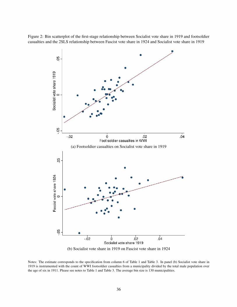
Figure 2: Bin scatterplot of the first-stage relationship between Socialist vote share in 1919 and footsoldiercasualties and the 2SLS relationship between Fascist vote share in 1924 and Socialist vote share in 1919

(a) Footsoldier casualties on Socialist vote share in 1919

(b) Socialist vote share in 1919 on Fascist vote share in 1924

Notes: The estimate corresponds to the specification from column 6 of Table 1 and Table 3. In panel (b) Socialist vote share in1919 is instrumented with the count of WWI footsoldier casualties from a municipality divided by the total male population overthe age of six in 1911. Please see notes to Table 1 and Table 3. The average bin size is 130 municipalities.

36

Figure 3: Bin scatterplot of the 2SLS relationship between Fascist violence and local branches and Socialistvote share in 1919

(a) Socialist vote share in 1919 on Fascist violence in 1920-22

(b) Socialist vote share in 1919 on Fascist local branches in 1921

Notes: The estimates correspond to the 2SLS specification from column 6 of Panel A and Panel B of Table 4. Socialist vote sharein 1919 is instrumented with footsoldier casualties. Please see notes to Table 4. The average bin size is 130 municipalities.

37

Table 1: The impact of footsoldier casualties in WWI on the Socialist vote share in 1919

Dep variable: Socialist vote share in 1919(1) (2) (3) (4) (5) (6)

Share of footsoldier casualties 2.034 1.953 1.772 1.752 1.686 1.689(0.315) (0.300) (0.236) (0.231) (0.230) (0.234)

Veterans (classes 1874-1895) 0.868 0.791 0.814(0.348) (0.353) (0.349)

Veterans (classes 1896-1900) -1.487 -1.411 -1.362(0.527) (0.547) (0.538)

Regiment/Province FE � � � � � �

Demographic controls � � � � � �

Geographic controls � � � � �

Socialist share in 1913 � � � �

Military controls � � �

Agriculture controls � �

Urban controls �

Observations 5,775 5,775 5,775 5,775 5,775 5,775R-squared 0.599 0.617 0.691 0.693 0.695 0.697Number of clusters 181 181 181 181 181 181F-stat 41.68 42.27 56.37 57.55 53.96 52.18Notes: The footsoldier casualty variable is the count of WWI footsoldier casualties from a municipality dividedby the total male population over the age of six in 1911. Column 1 includes regiment and province fixed effectsand demographic controls (quartic in log population and share of population below the age of six in 1911).Column 2 additionally includes geographic controls (log area, elevation of the main center, and maximumelevation). Column 3 adds Socialist vote share in 1913. Column 4 adds military controls (veterans fromclasses 1874-1895 and from classes 1896-1900 as well as dummies for any casualties of special assault corpsfrom the municipality, any casualties in the highest-mortality battles, and any casualties among volunteersfrom the municipality). Column 5 additionally includes agricultural controls (share of day laborers, share ofsharecroppers and a dummy for the presence of local agrarian associations). Finally, column 6 adds urbancontrols (industry workers and industrial firms over male population in 1911, literacy rate in 1911, the shareof entrepreneurs and rentiers, and the share of the bourgeoisie). See text for further details. Standard errorsclustered at the district level are in parentheses.

38

Table 2: Falsification exercises

(1) (2) (3) (4) (5) (6) (7) (8)

Panel A:Dep variable: Socialists 1913 Literacy 1911 Violent crimes 1874 Crime rate 1874

Share of footsoldier 0.185 0.227 -0.146 -0.194 0.504 0.094 5.734 2.213casualties (0.272) (0.250) (0.147) (0.142) (1.838) (1.850) (6.965) (6.504)

Mean 0.160 0.751 1.483 6.431SD 0.223 0.198 1.549 6.486

Panel B:Dep variable: Ind. workers 1911 Ind. firms 1911 Ind. strikes 1913-4 Ind. strikers 1913-4

Share of footsoldier -0.267 -0.284 0.021 0.024 0.002 0.007 -0.003 -0.003casualties (0.357) (0.351) (0.019) (0.017) (0.077) (0.077) (0.011) (0.011)

Mean 0.116 0.012 0.009 0.001SD 0.216 0.011 0.094 0.014

Panel C:Dep variable: Large landholding 1885 Landownership 1885 Agr. strikes 1913-4 Agr. strikers 1913-4

Share of footsoldier 0.236 0.335 0.485 0.525 -0.067 -0.079 0.005 0.002casualties (0.730) (0.678) (0.740) (0.664) (0.050) (0.054) (0.008) (0.008)

Mean 0.416 0.577 0.003 0.0004SD 0.495 0.494 0.056 0.011

Regiment/Province FE � � � � � � � �

Demographic controls � � � � � � � �

Geographic controls � � � � � � � �

Socialist share in 1913 � � � � � � � �

Military controls � � � � � � � �

Agriculture controls � � � �

Urban controls � � � �

Notes: OLS estimates of the relationship between the count of WWI footsoldier casualties from a municipality divided by the totalmale population over the age of six in 1911 and the indicated pre-1919 variables. The two specifications correspond to those fromcolumns 4 and 6 in Table 1. Column 4 includes regiment and province fixed effects and demographic controls (quartic in log populationand share of population below the age of six in 1911), geographic controls (log area, elevation of the main center, and maximumelevation), the Socialist vote share in 1913, and military controls (veterans from classes 1874-1895 and from classes 1896-1900 as wellas dummies for any casualties of special assault corps from the municipality, any casualties in the highest-mortality battles, and anycasualties among volunteers from the municipality). Column 6 additionally includes agricultural controls (share of day laborers, shareof sharecroppers and a dummy for the presence of local agrarian associations) and urban controls (industry workers and industrial firmsover male population in 1911, literacy rate in 1911, the share of entrepreneurs and rentiers, and the share of the bourgeoisie). See textfor details on dependent variables. We report mean and standard deviation (SD) of each dependent variable. When the left-hand sidevariable is among the controls included in one of the specifications, it is not included as an additional right-hand side variable. Standarderrors clustered at the district level are in parentheses.

39

Table 3: 2SLS estimates of the effects of Socialist vote share in 1919 on Fascist vote share in 1924

Dep variable: Fascist vote share in 1924(1) (2) (3) (4) (5) (6)

Panel A: IVSocialist vote share in 1919 0.375 0.429 0.476 0.504 0.489 0.476

(0.162) (0.153) (0.158) (0.156) (0.163) (0.156)

Panel B: OLSSocialist vote share in 1919 -0.016 0.011 0.019 0.024 0.019 0.022

(0.044) (0.039) (0.035) (0.032) (0.032) (0.032)

Regiment/Province FE � � � � � �

Demographic controls � � � � � �

Geographic controls � � � � �

Socialist share in 1913 � � � �

Military controls � � �

Agriculture controls � �

Urban controls �

Observations 5,775 5,775 5,775 5,775 5,775 5,775Number of clusters 181 181 181 181 181 181Notes: 2SLS (Panel A) and OLS (Panel B) regressions of the Fascist vote share in 1924 on the Socialistvote share in 1919. Excluded instrument is the count of WWI footsoldier casualties from a municipalitydivided by the total male population over the age of six in 1911. Column 1 includes regiment and provincefixed effects and demographic controls (quartic in log population and share of population below the age ofsix in 1911). Column 2 additionally includes geographic controls (log area, elevation of the main center,and maximum elevation). Column 3 adds Socialist vote share in 1913. Column 4 adds military controls(veterans from classes 1874-1895 and from classes 1896-1900 as well as dummies for any casualties ofspecial assault corps from the municipality, any casualties in the highest-mortality battles, and any casualtiesamong volunteers from the municipality). Column 5 additionally includes agricultural controls (share ofday laborers, share of sharecroppers and a dummy for the presence of local agrarian associations). Finallycolumn 6 adds urban controls (industry workers and industrial firms over male population in 1911, literacyrate in 1911, the share of entrepreneurs and rentiers, and the share of the bourgeoisie). Standard errorsclustered at the district level are in parentheses.

40

Table 4: 2SLS and OLS estimates of the effects of Socialist vote share in 1919 on Fascistviolence in 1920-22 and Fascist Party local branches in 1921

(1) (2) (3) (4) (5) (6)

Dep variable: Fascist violence in 1920-22 (episodes per 1000 inhabitants)

Panel A: IVSocialist vote share in 1919 0.230 0.239 0.254 0.329 0.311 0.312

(0.112) (0.116) (0.125) (0.126) (0.126) (0.122)

Panel B: OLSSocialist vote share in 1919 0.064 0.058 0.049 0.050 0.045 0.047

(0.014) (0.013) (0.015) (0.015) (0.014) (0.014)

Dep variable: Presence of local branches of the Fascist party in Fall 1921

Panel C: IVSocialist vote share in 1919 0.507 0.527 0.578 0.670 0.670 0.672

(0.227) (0.231) (0.257) (0.277) (0.277) (0.266)

Panel D: OLSSocialist vote share in 1919 0.080 0.072 0.081 0.086 0.080 0.083

(0.026) (0.026) (0.030) (0.030) (0.029) (0.028)

Regiment/Province FE � � � � � �

Demographic controls � � � � � �

Geographic controls � � � � �

Socialist share in 1913 � � � �

Military controls � � �

Agriculture controls � �

Urban controls �

Observations 5,775 5,775 5,775 5,775 5,775 5,775Number of clusters 181 181 181 181 181 181Notes: 2SLS and OLS regressions of the Fascist violence (episodes per 1000 inhabitants) in 1920-22 (PanelA and Panel B) and the presence of local Fascist branches in the Fall of 1921 (Panel C and Panel D) onthe Socialist vote share in 1919. Excluded instrument is the count of WWI footsoldier casualties from amunicipality divided by the total male population over the age of six in 1911. Column 1 includes regimentand province fixed effects and demographic controls (quartic in log population and share of population be-low the age of six in 1911). Column 2 additionally includes geographic controls (log area, elevation of themain center, and maximum elevation). Column 3 adds Socialist vote share in 1913. Column 4 adds militarycontrols (veterans from classes 1874-1895 and from classes 1896-1900 as well as dummies for any casual-ties of special assault corps from the municipality, any casualties in the highest-mortality battles, and anycasualties among volunteers from the municipality). Column 5 additionally includes agricultural controls(share of day laborers, share of sharecroppers and a dummy for the presence of local agrarian associations).Finally column 6 adds urban controls (industry workers and industrial firms over male population in 1911,literacy rate in 1911, the share of entrepreneurs and rentiers, and the share of the bourgeoisie). Standarderrors clustered at the district level are in parentheses.

41

Table 5: OLS estimates of the relationship between Socialist vote share in 1919 and agrarianstrikes in 1920

Dep variable: Agrarian strikes in 1920.(1) (2) (3) (4) (5) (6)

Socialist vote share in 1919 0.204 0.186 0.190 0.197 0.200 0.200(0.069) (0.070) (0.072) (0.073) (0.070) (0.071)

Regiment/Province FE � � � � � �

Demographic controls � � � � � �

Geographic controls � � � � �

Socialist share in 1913 � � � �

Military controls � � �

Agriculture controls � �

Urban controls �

Observations 5,775 5,775 5,775 5,775 5,775 5,775R-squared 0.777 0.778 0.778 0.779 0.784 0.785Number of clusters 181 181 181 181 181 181Notes: OLS regressions of agrarian strikes in 1920 on Socialist vote share in 1919. Column 1 includes regi-ment and province fixed effects and demographic controls (quartic in log population and share of populationbelow the age of six in 1911). Column 2 additionally includes geographic controls (log area, elevation ofthe main center, and maximum elevation). Column 3 adds Socialist vote share in 1913. Column 4 addsmilitary controls (veterans from classes 1874-1895 and from classes 1896-1900 as well as dummies for anycasualties of special assault corps from the municipality, any casualties in the highest-mortality battles, andany casualties among volunteers from the municipality). Column 5 additionally includes agricultural controls(share of day laborers, share of sharecroppers and a dummy for the presence of local agrarian associations).Finally column 6 adds urban controls (industry workers and industrial firms over male population in 1911,literacy rate in 1911, the share of entrepreneurs and rentiers, and the share of the bourgeoisie). Standard errorsclustered at the district level are in parentheses.

42

Table 6: 2SLS estimates of the relationship between Socialist vote share in 1919 and Socialistvote share in 1924

Dep variable: Socialist vote share in 1924(1) (2) (3) (4) (5) (6)

Socialist vote share in 1919 0.132 0.118 0.102 0.096 0.117 0.128(0.080) (0.078) (0.083) (0.084) (0.086) (0.084)

Regiment/Province FE � � � � � �

Demographic controls � � � � � �

Geographic controls � � � � �

Socialist share in 1913 � � � �

Military controls � � �

Agriculture controls � �

Urban controls �

Observations 5,775 5,775 5,775 5,775 5,775 5,775Number of clusters 181 181 181 181 181 181Notes: 2SLS regressions of the Socialist vote share in 1924 on the Socialist vote share in 1919. Excludedinstrument is the count of WWI footsoldier casualties from a municipality divided by the total male populationover the age of six in 1911. Column 1 includes regiment and province fixed effects and demographic controls(quartic in log population and share of population below the age of six in 1911). Column 2 additionallyincludes geographic controls (log area, elevation of the main center, and maximum elevation). Column 3adds Socialist vote share in 1913. Column 4 adds military controls (veterans from classes 1874-1895 andfrom classes 1896-1900 as well as dummies for any casualties of special assault corps from the municipality,any casualties in the highest-mortality battles, and any casualties among volunteers from the municipality).Column 5 additionally includes agricultural controls (share of day laborers, share of sharecroppers and adummy for the presence of local agrarian associations). Finally column 6 adds urban controls (industryworkers and industrial firms over male population in 1911, literacy rate in 1911, the share of entrepreneursand rentiers, and the share of the bourgeoisie). Standard errors clustered at the district level are in parentheses.

43

Table 7: Correlation between footsoldier casualties and support for Fascism and Nationalism

Per capita MonumentDep. Variable: Fascists 1919 Nationalists 1919 monuments 1921 1921 dummy

(1) (2) (3) (4) (5) (6) (7) (8)

Share of footsoldier casualties 0.069 0.065 -0.002 -0.002 -0.050 -0.046 -0.188 -0.130(0.050) (0.048) (0.004) (0.004) (0.334) (0.330) (0.264) (0.266)

Regiment/Province FE � � � � � � � �

Demographic controls � � � � � � � �

Geographic controls � � � � � � � �

Socialist share in 1913 � � � � � � � �

Military controls � � � � � � � �

Agriculture controls � � � �

Urban controls � � � �

Observations 5,775 5,775 5,775 5,775 5,775 5,775 5,775 5,775R-squared 0.251 0.257 0.496 0.496 0.091 0.093 0.211 0.214Number of clusters 181 181 181 181 181 181 181 181Notes: OLS estimates of the relationship between footsoldier casualties during WWI and the Fascist vote shares in 1919, the Nationalist

vote shares in 1919, the number of WWI monuments per 1000 inhabitants in the municipality between 1919 and 1921 and the indicator for

the erection of WWI monuments in the municipality between 1919 and 1921. The two specifications correspond to those from columns

4 and 6 in Table 1. Column 4 includes regiment and province fixed effects and demographic controls (quartic in log population and share

of population below the age of six in 1911), geographic controls (log area, elevation of the main center, and maximum elevation), the

Socialist vote share in 1913, and military controls (veterans from classes 1874-1895 and from classes 1896-1900 as well as dummies for

any casualties of special assault corps from the municipality, any casualties in the highest-mortality battles, and any casualties among

volunteers from the municipality). Column 6 additionally includes agricultural controls (share of day laborers, share of sharecroppers and

a dummy for the presence of local agrarian associations) and urban controls (industry workers and industrial firms over male population

in 1911, literacy rate in 1911, the share of entrepreneurs and rentiers, and the share of the bourgeoisie). Standard errors clustered at the

district level are in parentheses.

44

Table 8: Heterogeneous effects of Socialist vote share in 1919 on local Fascist support

Dep variable: Fascist vote share Fascist violence Fascist local branchin 1924 in 1920-2 in 1921

(1) (2) (3) (4) (5) (6)

Panel A: IV regressions for the presence of landowner associations

Socialist vote share in 1919 0.503 0.473 0.316 0.318 0.642 0.680(0.156) (0.155) (0.121) (0.120) (0.253) (0.257)

Socialists x landowner association dummy -0.442 -0.380 0.825 0.834 0.934 0.930(0.340) (0.319) (0.486) (0.474) (0.494) (0.487)

K-P F-stat 27.37 25.53 27.37 25.53 27.37 25.53

Panel B: IV regressions for the presence of elites (entrepreneurs and rentiers)

Socialist vote share in 1919 0.484 0.458 0.307 0.295 0.666 0.670(0.156) (0.165) (0.116) (0.117) (0.268) (0.264)

Socialists x elites 13.953 19.041 15.370 16.860 3.054 2.467(7.939) (9.185) (6.195) (7.623) (14.681) (16.731)

Kleibergen Paap F-stat 16.73 13.41 16.73 13.41 16.73 13.41

Panel C: Reduced-form regressions for the presence of landowner associations

Share of footsoldier casualties 0.876 0.803 0.532 0.507 1.094 1.109(0.264) (0.258) (0.202) (0.195) (0.423) (0.413)

Casualties x landowner association dummy -0.032 0.075 5.222 5.297 7.081 7.212(1.337) (1.346) (1.784) (1.729) (3.294) (3.294)

Panel D: Reduced-form regressions for the presence of elites (entrepreneurs and rentiers)

Share of footsoldier casualties 0.828 0.743 0.522 0.475 1.147 1.114(0.238) (0.238) (0.203) (0.192) (0.435) (0.403)

Casualties x elites 37.817 41.562 37.447 35.112 18.702 14.784(20.007) (19.138) (17.774) (17.375) (27.983) (27.126)

Regiment/Province FE � � � � � �

Demographic controls � � � � � �

Geographic controls � � � � � �

Socialist share in 1913 � � � � � �

Military controls � � � � � �

Agriculture controls � � �

Urban controls � � �

Observations 5,775 5,775 5,775 5,775 5,775 5,775Number of clusters 181 181 181 181 181 181Notes: 2SLS (Panels A and B) and reduced-form regressions (Panel C and D) of the heterogeneous effect of the Socialist vote share in 1919

on Fascism in the presence of landowners’ associations (Panel A and C) and the share of elites (Panel B and D). The endogenous variables are

Socialist vote share in 1919 and its interaction with the measure of elite organization. Excluded instruments are the count of WWI footsoldier

casualties from a municipality divided by the total male population over the age of six in 1911 and its interaction with the elite variables. The

left had side variables are the Fascist vote share in 1924 (columns 1 and 2), the Fascist violence (episodes per 1000 inhabitants) in 1920-22

(columns 3 and 4) and the presence of local Fascist branches in the Fall of 1921 (columns 5 and 6). The two specifications correspond to those

from columns 4 and 6 in Table 1. Column 4 includes regiment and province fixed effects and demographic controls (quartic in log population

and share of population below the age of six in 1911), geographic controls (log area, elevation of the main center, and maximum elevation),

the Socialist vote share in 1913, and military controls (veterans from classes 1874-1895 and from classes 1896-1900 as well as dummies for

any casualties of special assault corps from the municipality, any casualties in the highest-mortality battles, and any casualties among volunteers

from the municipality). Column 6 additionally includes agricultural controls (share of day laborers, share of sharecroppers and a dummy for the

presence of local agrarian associations) and urban controls (industry workers and industrial firms over male population in 1911, literacy rate in

1911, the share of entrepreneurs and rentiers, and the share of the bourgeoisie). Standard errors clustered at the district level are in parentheses.

45

Table 9: Results with alternative instruments: Spanish flu excess mortality in 1918 and relative rainfall in 1918-19

Dep variable: Socialist vote share Fascist vote share Fascist violence Fascist branchesin 1919 in 1924 in 1920-2 in 1921

(1) (2) (3) (4) (5) (6) (7) (8)

Panel A: Using excess mortality in 1918 as instrument

Excess mortality in 1918 0.093 0.097(0.028) (0.027)

Socialist vote share in 1919 0.599 0.738 0.054 -0.046 1.567 0.908(0.397) (0.428) (0.214) (0.195) (0.834) (0.756)

1st stage F-stat 10.78 12.84Observations 207 207 207 207 231 231 231 231Number of clusters 159 159 159 159 178 178 178 178

Panel B: Using rainfall in winter and spring 1818-1919 as instrument

Relative winter-spring -0.154 -0.148rainfall in 1918-9 (0.056) (0.057)Socialist vote share in 1919 0.711 0.784 -0.016 0.044 -0.259 -0.217

(0.372) (0.388) (0.134) (0.153) (0.274) (0.281)Rainfall variance � � � � � � � �

1st stage F-stat 6.957 6.209Observations 5,500 5,500 5,500 5,500 5,500 5,500 5,500 5,500Number of district clusters 174 174 174 174 174 174 174 174Number of station clusters 427 427 427 427 427 427 427 427

Regiment/Province FE � � � � � � � �

Demographic controls � � � � � � � �

Geographic controls � � � � � � � �

Socialist share in 1913 � � � � � � � �

Military controls � � � � � � � �

Agriculture controls � � � �

Urban controls � � � �

Notes: 2SLS regressions of the Fascist vote share in 1924 (columns 3 and 4), Fascist violence between 1920 and 1922 (columns 5 and

6) and Fascist branches in 1921 (columns 7 and 8) on the Socialist vote share in 1919. First stage results are reported in columns 1 and

2. In Panel A the excluded instrument is excess mortality due to the Spanish Flu in 1918. Excess mortality is defined as the excess

mortality in 1918 from the pre-war mortality computed between 1911 and 1914. In Panel B the excluded instrument is the relative

rainfall in winter-spring 1918-1919 (from December 1918 to May 1919). Relative rainfall is measured at weather station level, using

the average for the winter-spring months for the years 1915-1979 as denominator, and then interpolated at municipality level using the

inverse of the distances as weights with a cutoff of 30km. The relative rainfall measure is then capped at 1 in order to consider only

negative deviations from the long term average. The two specifications correspond to those from columns 4 and 6 in Table 1. Column

4 includes regiment and province fixed effects and demographic controls (quartic in log population and share of population below the

age of six in 1911), geographic controls (log area, elevation of the main center, and maximum elevation), the Socialist vote share in

1913, and military controls (veterans from classes 1874-1895 and from classes 1896-1900 as well as dummies for any casualties of

special assault corps from the municipality, any casualties in the highest-mortality battles, and any casualties among volunteers from

the municipality). Column 6 additionally includes agricultural controls (share of day laborers, share of sharecroppers and a dummy

for the presence of local agrarian associations) and urban controls (industry workers and industrial firms over male population in 1911,

literacy rate in 1911, the share of entrepreneurs and rentiers, and the share of the bourgeoisie). We report in parentheses standard errors

clustered at the district level (Panel A) and clustered over district and closest weather station (Panel B).

46

Table 10: 2SLS estimates of the effect of Fascist vote share in 1924 on Jewish deportations 1943-45

(1) (2) (3) (4) (5) (6)

Panel A: Jews deportation dummy (1943-45) - IV

Fascist vote share in 1924 0.884 0.810 0.817 0.805 0.866 0.862(0.462) (0.419) (0.416) (0.382) (0.427) (0.437)

Panel B: Deportations over Jewish population (capped at 1) - IV

Fascist vote share in 1924 0.886 0.817 0.815 0.787 0.854 0.844(0.412) (0.362) (0.357) (0.316) (0.359) (0.367)

Panel C: Deportations over Jewish population (cap at 1 no camps) - IV

Fascist vote share in 1924 0.783 0.727 0.721 0.694 0.751 0.744(0.382) (0.341) (0.334) (0.295) (0.335) (0.341)

Regiment/Province FE � � � � � �

Demographic controls � � � � � �

Share of jewish pop in 1911 � � � � � �

Geographic controls � � � � �

Socialist share in 1913 � � � �

Military controls � � �

Agriculture controls � �

Urban controls �

Observations 5,775 5,775 5,775 5,775 5,775 5,775Number of clusters 181 181 181 181 181 1811st Stage F-stat 6.467 9.095 9.714 11.13 9.510 9.649Notes: 2SLS regressions of: a dummy for the occurrence of Jews deportation in 1943-45 (Panel A); thenumber of deported Jews in 1943-45 over 1911 Jewish population, capped at 1 (Panel B); the number ofdeported Jews in 1943-45 over 1911 Jewish population, capped at 1 and excluding 39 municipalities withconcentration camps (Panel C) on the Fascist vote share in 1924. Excluded instrument is the count of WWIfootsoldier casualties from a municipality divided by the total male population over the age of six in 1911.Column 1 includes regiment and province fixed effects and demographic controls (quartic in log popula-tion and share of population below the age of six in 1911). Column 2 additionally includes geographiccontrols (log area, elevation of the main center, and maximum elevation). Column 3 adds Socialist voteshare in 1913. Column 4 adds military controls (veterans from classes 1874-1895 and from classes 1896-1900 as well as dummies for any casualties of special assault corps from the municipality, any casualtiesin the highest-mortality battles, and any casualties among volunteers from the municipality). Column 5additionally includes agricultural controls (share of day laborers, share of sharecroppers and a dummy forthe presence of local agrarian associations). Finally column 6 adds urban controls (industry workers andindustrial firms over male population in 1911, literacy rate in 1911, the share of entrepreneurs and rentiers,and the share of the bourgeoisie). Standard errors clustered at the district level are in parentheses.

47

Table 11: 2SLS estimates of the effect of Fascist vote share in 1924 on post-WWII party vote shares

Dep variable: Votes shares of(1) (2) (3) (4) (5) (6) (7) (8) (9) (10)

Panel A:

Left 0.443 1.081 0.791 0.839 0.654 0.563 0.400 0.495 0.651 0.543(0.191) (0.420) (0.338) (0.388) (0.320) (0.282) (0.233) (0.266) (0.310) (0.269)

Centre-right -0.434 -0.778 -0.616 -0.742 -0.647 -0.569 -0.630 -0.615 -0.606 -0.578(0.182) (0.327) (0.311) (0.327) (0.268) (0.272) (0.277) (0.288) (0.285) (0.270)

Extreme left 0.038 0.002 0.003 0.128 0.081 -0.004 0.037(0.020) (0.002) (0.004) (0.066) (0.049) (0.016) (0.015)

Extreme right 0.023 0.021 0.048 0.040 0.023 0.046 0.080 0.012 0.035(0.020) (0.039) (0.053) (0.032) (0.036) (0.033) (0.046) (0.036) (0.035)

Election(s): 1946-2018 1946 1948 1953 1958 1963 1968 1972 1976 1979Observations 109,725 5,775 5,775 5,775 5,775 5,775 5,775 5,775 5,775 5,775Number of clusters 5775 181 181 181 181 181 181 181 181 1811st Stage F-stat 9.871 9.668 9.668 9.668 9.668 9.668 9.668 9.668 9.668 9.668

Panel B:

Left 0.460 0.475 0.227 0.209 0.101 0.164 0.267 0.093 0.200 0.210(0.241) (0.240) (0.171) (0.116) (0.100) (0.120) (0.148) (0.056) (0.127) (0.122)

Centre-right -0.408 -0.516 -0.441 -0.304 -0.046 -0.171 -0.187 -0.100 -0.213 -0.079(0.229) (0.236) (0.226) (0.138) (0.099) (0.124) (0.119) (0.058) (0.151) (0.086)

Extreme left -0.022 -0.018 0.077 0.078 0.100 0.043 0.101 0.006 0.001 -0.003(0.014) (0.021) (0.054) (0.048) (0.060) (0.045) (0.056) (0.004) (0.003) (0.014)

Extreme right 0.045 0.007 0.013 0.006 -0.000 -0.015 0.013 0.005 0.007(0.046) (0.045) (0.037) (0.012) (0.010) (0.017) (0.008) (0.014) (0.012)

Election: 1983 1987 1992 1994 1996 2001 2006 2008 2013 2018Observations 5,775 5,775 5,775 5,775 5,775 5,775 5,775 5,775 5,775 5,775Number of clusters 181 181 181 181 181 181 181 181 181 1811st Stage F-stat 9.668 9.668 9.668 9.668 9.668 9.668 9.668 9.668 9.668 9.668

Full set of controls � � � � � � � � � �

Notes: 2SLS regressions of the vote shares of post-WWII parties for the period 1946-2018 on Fascist vote share in 1924. The left columnidentifies the party whose vote share is used as dependent variable in the regressions in each row. The heading Election identifies the election(s)included in the sample. The excluded instrument is the count of footsoldier casualties from a municipality divided by the total male populationover the age of six in 1911. All specifications include our full set of controls. We include regiment and province fixed effects and demographiccontrols (quartic in log population and share of population below the age of six in 1911), geographic controls (log area, elevation of themain center, and maximum elevation), the Socialist vote share in 1913, military controls (veterans from classes 1874-1895 and from classes1896-1900, dummies for any casualties of special assault corps from the municipality, any casualties in the highest-mortality battles, and anycasualties among volunteers from the municipality), agricultural controls (share of day laborers, share of sharecroppers and a dummy for thepresence of local agrarian associations) and urban controls (industry workers and industrial firms over male population in 1911, literacy rate in1911, the share of entrepreneurs and rentiers, and the share of the bourgeoisie). Standard errors clustered at the district level are in parenthesis.Column 1 of Panel A reports a pooled 2SLS regression for the period 1946-2018 where all controls are interacted with election dummies andstandard errors are clustered at the municipality level.

48

A Online Appendix (Not For Publication)

Figure A1: Example of newspaper source - Rinascita, April 11, 1924

A-1

Figure A2: Examples of archival sources

(a) Summary list from Pesaro-Urbino State Archive

(b) Telegraphic communication from Novara State Archive

A-2

Figure A3: Relative rainfall in winter-spring 1918-9

Notes: Relative rainfall in winter-spring 1918-9 using data from 427 weather stations gathered from the Hydrographic Bulletins(1915-1979) for the 16 Italian hydrographic compartments. Relative rainfall is measured at the weather station level (aggregatingrainfall from December 1918 to May 1919), using the average for the winter-spring months for the years 1915-1979 as denominator,and then interpolated at the municipality level using the inverse of the distances as weights with a cutoff of 30km. The blue shadingidentifies areas with more abundant rainfall in winter-spring 1918-9 as compared to their usual rainfall pattern. Orange, red, andbrown shadings identify progressively lower rainfall in winter-spring 1918-9 as compared to their usual rainfall pattern. Black dotsdenote the location of weather stations.

A-3

Table A1: Descriptive statistics

Variable Obs Mean Std. Dev. Min MaxDependent variables:Fascist vote share in 1924 5,775 0.619 0.257 0 1Fascist violence in 1920-2 5,775 .042 0.164 0 2.225Fascist local branches in Autumn 1921 5,775 0.145 0.352 0 1Agrarian Strikes in 1920 5,775 0.303 0.600 0 4Jews deportation dummy (1943-45) 5,775 0.070 0.255 0 1Deportations over Jewish population (capped at 1) 5,775 0.050 0.21 0 1Deportations over Jewish population (cap at 1 no camps) 5,736 0.044 0.197 0 1Left vote share (1946-2018) 109,725 0.224 0.134 0 0.880Centre-right vote share (1946-2018) 109,725 0.363 0.179 0 0.992Extreme right vote share (1946-2018) 98,175 0.026 0.029 0 0.729Extreme left vote share (1946-2018) 92,400 0.029 0.032 0 0.632

Main excluded instruments:Foot-soldier casualties over male pop above 6 5,775 0.032 0.016 0 0.385Excess mortality in 1918 231 0.892 0.387 -0.191 3.482Relative winter-spring rainfall 1918-9 5,500 0.849 0.166 0.213 1

Socialist support:Socialist vote share in 1913 5,775 0.160 0.223 0 1Socialist vote share in 1919 5,775 0.316 0.271 0 1Socialist (+ Communist) vote share in 1921 5,083 0.258 0.227 0 1Socialist (+ Communist) vote share in 1924 5,751 0.152 0.153 0 0.866

Demographic controls:(log) Population in 1911 5,775 7.653 1.071 3.970 13.427Share of below 6 population in 1911 5,775 0.158 0.033 0.054 0.928

Geographic controls:(log) Municipality area 5,775 7.454 1.133 2.303 12.243Elevation of the major centre 5,775 318.195 280.476 1 1816Maximum elevation 5,775 836.126 840.759 1 4810

Military controls:Dummy for casualties in assault troops 5,775 0.238 0.426 0 1Dummy for casualties in voluntary troops 5,775 0.013 0.112 0 1Dummy for casualties in deadly battles 5,775 0.960 0.195 0 1Veterans (classes 1874-1895) over male pop above 6 in 1911 5,775 0.234 0.057 0.099 0.406Veterans (classes 1896-1900) over male pop above 6 in 1911 5,775 0.132 0.023 0.069 0.204

Agriculture controls:Share of day labourers in 1921 5,775 0.214 0.118 0.010 0.678Share of share-croppers in 1921 5,775 0.052 0.071 0 0.421Landowner association dummy 5,775 0.050 0.218 0 1

Urban controls:Industrial workers over male population in 1911 5,775 0.116 0.216 0 6.028Industry firms over male population in 1911 5,775 0.012 0.011 0 0.138Male literacy in 1911 5,775 0.751 0.198 0.101 1Share of elites (entrepreneurs and rentiers) in 1921 5,775 0.026 0.012 0 0.088Share of bourgeoisie in 1921 5,775 0.085 0.032 0.028 0.240

A-4

Table A2: 2SLS estimates of the effects of Socialist vote share in 1919 on measures of Fascist support using spatially-corrected(Conley) standard errors

Dep variable: Socialist vote share Fascist vote share Fascist branches Fascist violencein 1919 in 1924 in 1921 in 1920-2

(1) (2) (3) (4) (5) (6) (7) (8)

Share of footsoldier casualties 1.752 1.689(0.252) (0.248)

Socialist vote share in 1919 0.504 0.476 0.329 0.312 0.670 0.672(0.131) (0.139) (0.142) (0.126) (0.275) (0.227)

Regiment/Province FE � � � � � � � �

Demographic controls � � � � � � � �

Geographic controls � � � � � � � �

Socialist share in 1913 � � � � � � � �

Military controls � � � � � � � �

Agriculture controls � � � �

Urban controls � � � �

1st stage F-stat 48.34 46.38Observations 5,775 5,775 5,775 5,775 5,775 5,775 5,775 5,775Notes: 2SLS regressions of the Fascist vote share in 1924 (columns 3 and 4), Fascist branches in 1921 (columns 5 and 6) and Fascist

violence between 1920 and 1922 (columns 7 and 8) on the Socialist vote share in 1919. First stage results are reported in columns 1 and

2. The excluded instrument is the count of footsoldier casualties from a municipality divided by the total male population over the age of

six in 1911. The two specifications correspond to those from columns 4 and 6 in Table 1. Column 4 includes regiment and province fixed

effects and demographic controls (quartic in log population and share of population below the age of six in 1911), geographic controls (log

area, elevation of the main center, and maximum elevation), the Socialist vote share in 1913, and military controls (veterans from classes

1874-1895 and from classes 1896-1900 as well as dummies for any casualties of special assault corps from the municipality, any casualties

in the highest-mortality battles, and any casualties among volunteers from the municipality). Column 6 additionally includes agricultural

controls (share of day laborers, share of sharecroppers and a dummy for the presence of local agrarian associations) and urban controls

(industry workers and industrial firms over male population in 1911, literacy rate in 1911, the share of entrepreneurs and rentiers, and the

share of the bourgeoisie). Spatially-corrected (Conley) standard errors with cutoffs at 1.5 degrees for both latitude and longitude are in

parentheses.

A-5

Table A3: First-stage estimates using alternative definitions of our casualties instrument

Dep variable: Socialist vote share in 1919(1) (2) (3) (4) (5) (6)

Casualties among reservist & 1.622 1.563drafted footsoldiers (0.213) (0.214)

Casualties among drafted 2.002 1.860footsoldiers (0.303) (0.303)

Casualties among 1.250 1.210all soldiers (0.162) (0.158)

Regiment/Province FE � � � � � �

Demographic controls � � � � � �

Geographic controls � � � � � �

Socialist share in 1913 � � � � � �

Military controls � � � � � �

Agriculture controls � � �

Urban controls � � �

Observations 5,775 5,775 5,775 5,775 5,775 5,775R-squared 0.693 0.696 0.691 0.694 0.693 0.696Number of clusters 181 181 181 181 181 181F-stat 57.87 53.16 43.58 37.72 59.84 58.67Notes: First-stage regression using alternative measures of casualties. In columns 1 and 2 excluded instru-

ment is defined using the number of casualties from men drafted and reservists. Columns 3 and 4 use only

the number of casualties from men drafted to construct the excluded instrument while columns 5 and 6 use

casualties from all soldiers. All versions of the instruments are computed in shares, dividing the number of

casualties with the total male population over six years old in 1911. The two specifications correspond to

those from columns 4 and 6 in Table 1. Column 4 includes regiment and province fixed effects and demo-

graphic controls (quartic in log population and share of population below the age of six in 1911), geographic

controls (log area, elevation of the main center, and maximum elevation), the Socialist vote share in 1913, and

military controls (veterans from classes 1874-1895 and from classes 1896-1900 as well as dummies for any

casualties of special assault corps from the municipality, any casualties in the highest-mortality battles, and

any casualties among volunteers from the municipality). Column 6 additionally includes agricultural controls

(share of day laborers, share of sharecroppers and a dummy for the presence of local agrarian associations)

and urban controls (industry workers and industrial firms over male population in 1911, literacy rate in 1911,

the share of entrepreneurs and rentiers, and the share of the bourgeoisie). Standard errors clustered at the

district level are in parentheses.

A-6

Table A4: 2SLS estimates of the effects of Socialist vote share in 1919 on Fascist vote share in1924 controlling for Fascist vote share in 1919

Dep variable: Fascist vote share in 1924(1) (2) (3) (4) (5) (6)

Socialist vote share in 1919 0.373 0.426 0.473 0.493 0.478 0.463(0.161) (0.152) (0.156) (0.152) (0.159) (0.152)

Fascist share in 1919 0.138 0.336 0.333 0.293 0.287 0.318(0.161) (0.119) (0.121) (0.122) (0.123) (0.125)

Regiment/Province FE � � � � � �

Demographic controls � � � � � �

Geographic controls � � � � �

Socialist share in 1913 � � � �

Military controls � � �

Agriculture controls � �

Urban controls �

Observations 5,775 5,775 5,775 5,775 5,775 5,775Number of clusters 181 181 181 181 181 1811st Stage F-stat 41.93 42.70 57.31 58 54.55 52.83Notes: 2SLS regressions of the Fascist vote share in 1924 on the Socialist vote share in 1919 controllingfor Fascist vote share in 1919. The excluded instrument is the count of footsoldier casualties from a munic-ipality divided by the total male population over the age of six in 1911. Column 1 includes regiment andprovince fixed effects and demographic controls (quartic in log population and share of population belowthe age of six in 1911). Column 2 additionally includes geographic controls (log area, elevation of the maincenter, and maximum elevation). Column 3 adds Socialist vote share in 1913. Column 4 adds militarycontrols (veterans from classes 1874-1895 and from classes 1896-1900 as well as dummies for any casual-ties of special assault corps from the municipality, any casualties in the highest-mortality battles, and anycasualties among volunteers from the municipality). Column 5 additionally includes agricultural controls(share of day laborers, share of sharecroppers and a dummy for the presence of local agrarian associations).Finally column 6 adds urban controls (industry workers and industrial firms over male population in 1911,literacy rate in 1911, the share of entrepreneurs and rentiers, and the share of the bourgeoisie). Standarderrors clustered at the district level are in parentheses.

A-7

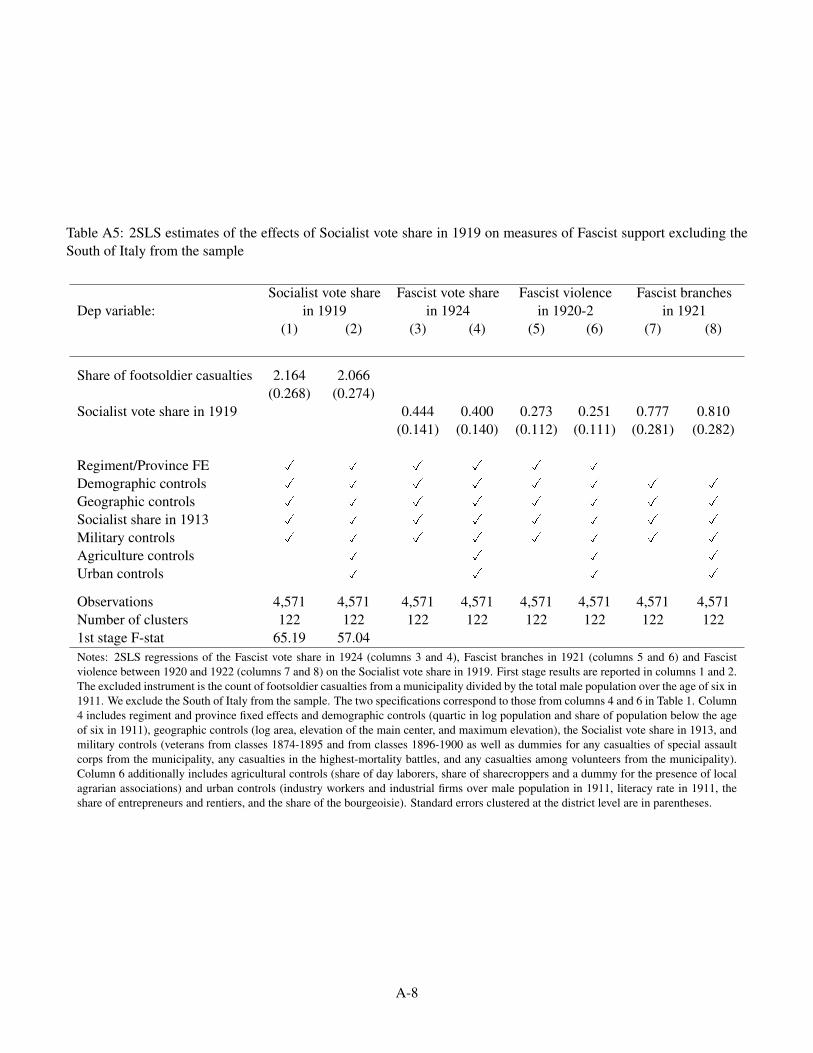
Table A5: 2SLS estimates of the effects of Socialist vote share in 1919 on measures of Fascist support excluding theSouth of Italy from the sample

Socialist vote share Fascist vote share Fascist violence Fascist branchesDep variable: in 1919 in 1924 in 1920-2 in 1921

(1) (2) (3) (4) (5) (6) (7) (8)

Share of footsoldier casualties 2.164 2.066(0.268) (0.274)

Socialist vote share in 1919 0.444 0.400 0.273 0.251 0.777 0.810(0.141) (0.140) (0.112) (0.111) (0.281) (0.282)

Regiment/Province FE � � � � � �

Demographic controls � � � � � � � �

Geographic controls � � � � � � � �

Socialist share in 1913 � � � � � � � �

Military controls � � � � � � � �

Agriculture controls � � � �

Urban controls � � � �

Observations 4,571 4,571 4,571 4,571 4,571 4,571 4,571 4,571Number of clusters 122 122 122 122 122 122 122 1221st stage F-stat 65.19 57.04Notes: 2SLS regressions of the Fascist vote share in 1924 (columns 3 and 4), Fascist branches in 1921 (columns 5 and 6) and Fascistviolence between 1920 and 1922 (columns 7 and 8) on the Socialist vote share in 1919. First stage results are reported in columns 1 and 2.The excluded instrument is the count of footsoldier casualties from a municipality divided by the total male population over the age of six in1911. We exclude the South of Italy from the sample. The two specifications correspond to those from columns 4 and 6 in Table 1. Column4 includes regiment and province fixed effects and demographic controls (quartic in log population and share of population below the ageof six in 1911), geographic controls (log area, elevation of the main center, and maximum elevation), the Socialist vote share in 1913, andmilitary controls (veterans from classes 1874-1895 and from classes 1896-1900 as well as dummies for any casualties of special assaultcorps from the municipality, any casualties in the highest-mortality battles, and any casualties among volunteers from the municipality).Column 6 additionally includes agricultural controls (share of day laborers, share of sharecroppers and a dummy for the presence of localagrarian associations) and urban controls (industry workers and industrial firms over male population in 1911, literacy rate in 1911, theshare of entrepreneurs and rentiers, and the share of the bourgeoisie). Standard errors clustered at the district level are in parentheses.

A-8

Table A6: 2SLS estimates of the effects of Socialist vote share in 1919 on Fascist vote share in 1924 definedusing only the official lists

Dep variable: Fascist vote share in 1924 (official lists only)(1) (2) (3) (4) (5) (6)

Socialist vote share in 1919 0.317 0.369 0.408 0.434 0.419 0.407(0.166) (0.159) (0.167) (0.165) (0.171) (0.164)

Regiment/Province FE � � � � � �

Demographic controls � � � � � �

Geographic controls � � � � �

Socialist share in 1913 � � � �

Military controls � � �

Agriculture controls � �

Urban controls �

Observations 5,775 5,775 5,775 5,775 5,775 5,775Number of clusters 181 181 181 181 181 181Notes: 2SLS regressions of the Fascist vote share in 1924 (only official lists) on the Socialist vote sharein 1919. The excluded instrument in the first stage is the count of footsoldier casualties during WWI overmale population over six years old in 1911. Column 1 includes regiment and province fixed effects anddemographic controls (quartic in log population and share of population below the age of six in 1911).Column 2 additionally includes geographic controls (log area, elevation of the main center, and maximumelevation). Column 3 adds Socialist vote share in 1913. Column 4 adds military controls (veterans fromclasses 1874-1895 and from classes 1896-1900 as well as dummies for any casualties of special assaultcorps from the municipality, any casualties in the highest-mortality battles, and any casualties among vol-unteers from the municipality). Column 5 additionally includes agricultural controls (share of day laborers,share of sharecroppers and a dummy for the presence of local agrarian associations). Finally column 6 addsurban controls (industry workers and industrial firms over male population in 1911, literacy rate in 1911,the share of entrepreneurs and rentiers, and the share of the bourgeoisie). Standard errors clustered at thedistrict level are in parentheses.

A-9

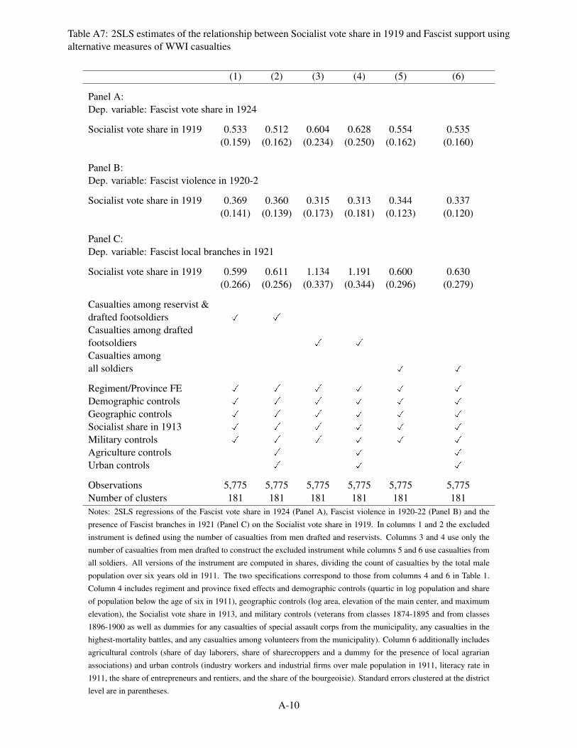
Table A7: 2SLS estimates of the relationship between Socialist vote share in 1919 and Fascist support usingalternative measures of WWI casualties

(1) (2) (3) (4) (5) (6)

Panel A:Dep. variable: Fascist vote share in 1924

Socialist vote share in 1919 0.533 0.512 0.604 0.628 0.554 0.535(0.159) (0.162) (0.234) (0.250) (0.162) (0.160)

Panel B:Dep. variable: Fascist violence in 1920-2

Socialist vote share in 1919 0.369 0.360 0.315 0.313 0.344 0.337(0.141) (0.139) (0.173) (0.181) (0.123) (0.120)

Panel C:Dep. variable: Fascist local branches in 1921

Socialist vote share in 1919 0.599 0.611 1.134 1.191 0.600 0.630(0.266) (0.256) (0.337) (0.344) (0.296) (0.279)

Casualties among reservist &drafted footsoldiers � �

Casualties among draftedfootsoldiers � �

Casualties amongall soldiers � �

Regiment/Province FE � � � � � �

Demographic controls � � � � � �

Geographic controls � � � � � �

Socialist share in 1913 � � � � � �

Military controls � � � � � �

Agriculture controls � � �

Urban controls � � �

Observations 5,775 5,775 5,775 5,775 5,775 5,775Number of clusters 181 181 181 181 181 181Notes: 2SLS regressions of the Fascist vote share in 1924 (Panel A), Fascist violence in 1920-22 (Panel B) and the

presence of Fascist branches in 1921 (Panel C) on the Socialist vote share in 1919. In columns 1 and 2 the excluded

instrument is defined using the number of casualties from men drafted and reservists. Columns 3 and 4 use only the

number of casualties from men drafted to construct the excluded instrument while columns 5 and 6 use casualties from

all soldiers. All versions of the instrument are computed in shares, dividing the count of casualties by the total male

population over six years old in 1911. The two specifications correspond to those from columns 4 and 6 in Table 1.

Column 4 includes regiment and province fixed effects and demographic controls (quartic in log population and share

of population below the age of six in 1911), geographic controls (log area, elevation of the main center, and maximum

elevation), the Socialist vote share in 1913, and military controls (veterans from classes 1874-1895 and from classes

1896-1900 as well as dummies for any casualties of special assault corps from the municipality, any casualties in the

highest-mortality battles, and any casualties among volunteers from the municipality). Column 6 additionally includes

agricultural controls (share of day laborers, share of sharecroppers and a dummy for the presence of local agrarian

associations) and urban controls (industry workers and industrial firms over male population in 1911, literacy rate in

1911, the share of entrepreneurs and rentiers, and the share of the bourgeoisie). Standard errors clustered at the district

level are in parentheses.

A-10

Table A8: 2SLS estimates of the relationship between Socialist vote share in 1919, Fascist votes in 1921elections and alternative definitions of Fascist violence

(1) (2) (3) (4) (5) (6)

Panel A: Fascist vote Fascist vote Fascist and NationalDep variable: share in 1921 in 1921 dummy Blocks share in 1921

Socialist vote share in 1919 0.013 0.013 0.052 0.054 -0.154 -0.190(0.007) (0.007) (0.026) (0.028) (0.181) (0.172)

Observations 5,084 5,084 5,084 5,084 5,084 5,084Number of clusters 172 172 172 172 172 172

Panel B: Fascist killings Political violence Non-fascist violenceDep variable: in 1920-2 in 1920-2 in 1920-2

Socialist vote share in 1919 0.091 0.093 0.326 0.307 -0.006 -0.008(0.046) (0.045) (0.128) (0.123) (0.021) (0.021)

Observations 5,775 5,775 5,775 5,775 5,775 5,775Number of clusters 181 181 181 181 181 181

Regiment/Province FE � � � � � �

Demographic controls � � � � � �

Geographic controls � � � � � �

Socialist share in 1913 � � � � � �

Military controls � � � � � �

Agriculture controls � � �

Urban controls � � �

Notes: 2SLS regressions of alternative measure of the Fascist vote share in 1921 (Panel A) and alternative

measures of Fascist violence in 1920-22 (Panel B) on the Socialist vote share in 1919. The left-hand side vari-

ables in Panel A are: the Fascist vote share in 1921, a dummy for Fascists receiving a positive number of votes

in 1921, and the aggregate vote share of Fascists and National blocks in 1921. In Panel B we consider: the

number of killings per 1000 inhabitants in 1920-2 perpetrated by Fascists, the number of violent episodes per

1000 inhabitants in 1920-2 by any perpetrator, and the number of violent episodes excluding Fascist violence.

The two specifications correspond to those from columns 4 and 6 in Table 1. Column 4 includes regiment and

province fixed effects and demographic controls (quartic in log population and share of population below the

age of six in 1911), geographic controls (log area, elevation of the main center, and maximum elevation), the

Socialist vote share in 1913, and military controls (veterans from classes 1874-1895 and from classes 1896-

1900 as well as dummies for any casualties of special assault corps from the municipality, any casualties in the

highest-mortality battles, and any casualties among volunteers from the municipality). Column 6 additionally

includes agricultural controls (share of day laborers, share of sharecroppers and a dummy for the presence of

local agrarian associations) and urban controls (industry workers and industrial firms over male population in

1911, literacy rate in 1911, the share of entrepreneurs and rentiers, and the share of the bourgeoisie). Standard

errors clustered at the district level are in parentheses.

A-11

Table A9: 2SLS estimates of the relationship between Socialist vote share in 1919 and Fascist support using alternative fixed effects specifications

Dep. variable: Fascist vote share in 1924 Fascist violence in 1920-2 Fascist local branches in 1921

(1) (2) (3) (4) (5) (6) (7) (8) (9) (10) (11) (12)

Socialist vote share in 1919 0.457 0.406 0.391 0.352 0.316 0.281 0.305 0.281 0.700 0.655 0.683 0.664(0.174) (0.168) (0.159) (0.159) (0.131) (0.119) (0.131) (0.122) (0.307) (0.276) (0.330) (0.311)

Province FE � � � � � � � � � � � �

Demographic controls � � � � � � � � � � � �

Geographic controls � � � � � � � � � � � �

Socialist share in 1913 � � � � � � � � � � � �

Military controls � � � � � � � � � � � �

Agriculture controls � � � � � �

Urban controls � � � � � �

Front Semester FE � � � � � �

Front Month FE � � � � � �

Observations 5,775 5,775 5,775 5,775 5,775 5,775 5,775 5,775 5,775 5,775 5,775 5,775Number of clusters 181 181 181 181 181 181 181 181 181 181 181 1811st Stage F-stat 42.17 42.45 39.72 37.74 42.17 42.45 39.72 37.74 42.17 42.45 39.72 37.74Notes: 2SLS regressions of the Fascist vote share in 1924 (columns 1 to 4), Fascist violence in 1920-22 (columns 5 to 8) and the presence of Fascist branches in 1921 (columns9 to 12) on the Socialist vote share in 1919. Excluded instrument is the count of footsoldier casualties from a municipality divided by the total male population over the age ofsix in 1911. The two specifications correspond to those from columns 4 and 6 in Table 1 except for regiment fixed effects replaced by either front-semester fixed effects (columns1-2, 5-6, 9-10) or front-month fixed effects (columns 3-4, 7-8, 11-12). Column 4 includes province fixed effects and demographic controls (quartic in log population and shareof population below the age of six in 1911), geographic controls (log area, elevation of the main center, and maximum elevation), the Socialist vote share in 1913, and militarycontrols (veterans from classes 1874-1895 and from classes 1896-1900 as well as dummies for any casualties of special assault corps from the municipality, any casualties inthe highest-mortality battles, and any casualties among volunteers from the municipality). Column 6 additionally includes agricultural controls (share of day laborers, share ofsharecroppers and a dummy for the presence of local agrarian associations) and urban controls (industry workers and industrial firms over male population in 1911, literacy rate in1911, the share of entrepreneurs and rentiers, and the share of the bourgeoisie). Standard errors clustered at the district level are in parentheses.

A-12

Table A10: 2SLS estimates of the effects of Socialist vote share in 1919 on vote share of other main parties in 1924

Dep. variable: Party’s vote share in 1924(1) (2) (3) (4) (5) (6) (7) (8) (9) (10) (11) (12)

Panel A: Controlling for 1919 vote shares

Socialist vote share in 1919 -0.155 -0.122 -0.003 -0.009 0.012 0.008 0.005 0.009 -0.279 -0.294 0.000 -0.007(0.131) (0.123) (0.017) (0.020) (0.044) (0.046) (0.052) (0.054) (0.072) (0.078) (0.020) (0.022)

Vote share in 1919 0.229 0.239 0.389 0.383 0.018 0.016 0.018 0.019 -0.206 -0.211 0.018 0.017(0.067) (0.064) (0.032) (0.031) (0.020) (0.021) (0.015) (0.014) (0.076) (0.075) (0.016) (0.016)

Panel B: No control for 1919 party vote shares

Socialist vote share in 1919 -0.308 -0.273 0.003 -0.003 0.013 0.011 0.010 0.014 -0.276 -0.294 0.003 -0.004(0.110) (0.104) (0.017) (0.020) (0.036) (0.037) (0.055) (0.056) (0.071) (0.078) (0.021) (0.022)

Party considered: Popular Republican Democratic Liberal Agrarian Left LiberalMean vote share in 1919 0.272 0.004 0.222 0.096 0.009 0.011Regiment/Province FE � � � � � � � � � � � �

Demographic controls � � � � � � � � � � � �

Geographic controls � � � � � � � � � � � �

Socialist share in 1913 � � � � � � � � � � � �

Military controls � � � � � � � � � � � �

Agriculture controls � � � � � �

Urban controls � � � � � �

Notes: 2SLS regressions of the vote shares of other main parties competing in the 1924 national elections other than the Fascist party on Socialist vote share in 1919. Panel A presentsresults controlling for the same party electoral share in 1919, while Panel B presents results without controlling for the party 1919 electoral share. We also report the mean vote shareof each party in 1919. The two specifications correspond to those from columns 4 and 6 in Table 1. Column 4 includes regiment and province fixed effects and demographic controls(quartic in log population and share of population below the age of six in 1911), geographic controls (log area, elevation of the main center, and maximum elevation), the Socialist voteshare in 1913, and military controls (veterans from classes 1874-1895 and from classes 1896-1900 as well as dummies for any casualties of special assault corps from the municipality,any casualties in the highest-mortality battles, and any casualties among volunteers from the municipality). Column 6 additionally includes agricultural controls (share of day laborers,share of sharecroppers and a dummy for the presence of local agrarian associations) and urban controls (industry workers and industrial firms over male population in 1911, literacyrate in 1911, the share of entrepreneurs and rentiers, and the share of the bourgeoisie). Standard errors clustered at the district level are in parentheses.

A-13

Table A11: Heterogeneous effects of Socialist vote share in 1919 on thepresence of large donors for the Fascist party

Dep variable: Large donor dummy (1919-25)(1) (2) (3) (4)

Socialist vote share in 1919 0.013 0.033 -0.005 0.020(0.095) (0.096) (0.102) (0.105)

Socialists x elite variable 0.438 0.421 8.555 10.783(0.217) (0.209) (5.606) (6.472)

Elite variable Landowner Share ofass. dummy elites

Regiment/Province FE � � � �

Demographic controls � � � �

Geographic controls � � � �

Socialist share in 1913 � � � �

Military controls � � � �

Agriculture controls � �

Urban controls � �

Observations 5,775 5,775 5,775 5,775Number of clusters 181 181 181 181Kleibergen Paap F-stat 27.37 25.53 16.73 13.41Notes: 2SLS regressions of the heterogeneous effect of the Socialist vote share in

1919 on a dummy for the presence of large donors to the Fascist Party in the pe-

riod 1919-1925 in the presence of landowners’ associations (columns 1 and 2) and

the share of elites (columns 3 and 4). The endogenous variables are Socialist vote

share in 1919 and its interaction with the measure of elite organization. Excluded

instruments are the count of WWI footsoldier casualties from a municipality di-

vided by the total male population over the age of six in 1911 and its interaction

with the elite variables. The two specifications correspond to those from columns

4 and 6 in Table 1. Column 4 includes regiment and province fixed effects and de-

mographic controls (quartic in log population and share of population below the

age of six in 1911), geographic controls (log area, elevation of the main center,

and maximum elevation), the Socialist vote share in 1913, and military controls

(veterans from classes 1874-1895 and from classes 1896-1900 as well as dummies

for any casualties of special assault corps from the municipality, any casualties in

the highest-mortality battles, and any casualties among volunteers from the mu-

nicipality). Column 6 additionally includes agricultural controls (share of day

laborers, share of sharecroppers and a dummy for the presence of local agrarian

associations) and urban controls (industry workers and industrial firms over male

population in 1911, literacy rate in 1911, the share of entrepreneurs and rentiers,

and the share of the bourgeoisie). Standard errors clustered at the district level are

in parentheses.

A-14

Table A12: Reduced-form estimates of the relationship between footsoldier casualties and measures of localFascist support

Dep variable: Fascist vote share Fascist violence Fascist branchesin 1924 in 1920-2 in 1921

(1) (2) (3) (4) (5) (6)

Share of footsoldier casualties 0.883 0.804 0.576 0.526 1.175 1.135(0.264) (0.258) (0.214) (0.200) (0.463) (0.418)

Regiment/Province FE � � � � � �

Demographic controls � � � � � �

Geographic controls � � � � � �

Socialist share in 1913 � � � � � �

Military controls � � � � � �

Agriculture controls � � �

Urban controls � � �

Observations 5,775 5,775 5,775 5,775 5,775 5,775Number of clusters 181 181 181 181 181 181Notes: Reduced-form regressions of the Fascist vote share in 1924 (columns 1 and 2), Fascist violence between

1920 and 1922 (columns 3 and 4) and Fascist branches in 1921 (columns 5 and 6) on the count of footsoldier

casualties during WWI over male population over six years old in 1911. The two specifications correspond to

those from columns 4 and 6 in Table 1. Column 4 includes regiment and province fixed effects and demographic

controls (quartic in log population and share of population below the age of six in 1911), geographic controls

(log area, elevation of the main center, and maximum elevation), the Socialist vote share in 1913, and military

controls (veterans from classes 1874-1895 and from classes 1896-1900 as well as dummies for any casualties

of special assault corps from the municipality, any casualties in the highest-mortality battles, and any casual-

ties among volunteers from the municipality). Column 6 additionally includes agricultural controls (share of

day laborers, share of sharecroppers and a dummy for the presence of local agrarian associations) and urban

controls (industry workers and industrial firms over male population in 1911, literacy rate in 1911, the share of

entrepreneurs and rentiers, and the share of the bourgeoisie). Standard errors clustered at the district level are

in parentheses.

A-15

Table A13: Falsification exercises for the Spanish flu excess mortality

(1) (2) (3) (4) (5) (6) (7) (8)

Panel A:Dep variable: Socialists in 1913 Literacy in 1911 Violent crimes in 1874 Crime rate in 1874

Excess Mortality in 1918 -0.027 -0.045 0.033 0.022 0.285 0.352 -1.351 -1.399(0.035) (0.035) (0.017) (0.016) (0.236) (0.240) (1.031) (1.007)

Mean 0.207 0.685 1.932 8.174SD 0.217 0.188 1.576 5.840

Panel B:Dep variable: Ind. workers in 1911 Ind. firms in 1911 Ind. strikes in 1913-4 Ind. strikers in 1913-4

Excess Mortality in 1918 0.039 0.019 0.001 0.000 -0.129 -0.146 -0.000 -0.000(0.017) (0.017) (0.002) (0.002) (0.066) (0.073) (0.000) (0.000)

Mean 0.185 0.018 0.106 0.0005SD 0.162 0.008 0.309 0.003

Panel C:Dep variable: Large landhold. Many landowners Agr. strikes in 1913-4 Agr. strikers in 1913-4

Excess Mortality in 1918 0.011 0.053 0.132 0.117 -0.012 -0.002 0.001 0.002(0.112) (0.112) (0.095) (0.098) (0.014) (0.016) (0.002) (0.003)

Mean 0.391 0.454 0.015 0.001SD 0.489 0.499 0.120 0.019

Regiment/Province FE � � � � � � � �

Rainfall variance � � � � � � � �

Demographic controls � � � � � � � �

Geographic controls � � � � � � � �

Socialist share in 1913 � � � � � � � �

Military controls � � � � � � � �

Agriculture controls � � � �

Urban controls � � � �

Notes: OLS regressions of the indicated pre-1919 variable on the excess mortality in 1918. Excess mortality is defined as the excess mortality in

1918 from the pre-war mortality computed between 1911 and 1914. The two specifications correspond to those from columns 4 and 6 in Table 1.

Column 4 includes regiment and province fixed effects and demographic controls (quartic in log population and share of population below the age

of six in 1911), geographic controls (log area, elevation of the main center, and maximum elevation), the Socialist vote share in 1913, and military

controls (veterans from classes 1874-1895 and from classes 1896-1900 as well as dummies for any casualties of special assault corps from the

municipality, any casualties in the highest-mortality battles, and any casualties among volunteers from the municipality). Column 6 additionally

includes agricultural controls (share of day laborers, share of sharecroppers and a dummy for the presence of local agrarian associations) and urban

controls (industry workers and industrial firms over male population in 1911, literacy rate in 1911, the share of entrepreneurs and rentiers, and the

share of the bourgeoisie). See note to Table 1 and the text for more details. When the left-hand side variable is among the controls included in one

of the specifications, it is not included as an additional right-hand side variable. Standard errors clustered at the district level are in parentheses.

A-16

Table A14: Falsification exercises of winter-spring rainfall in 1918-19

(1) (2) (3) (4) (5) (6) (7) (8)

Panel A:Dep variable: Socialists in 1913 Literacy in 1911 Violent crimes in 1874 Crime rate in 1874

Relative winter-spring -0.223 -0.216 -0.041 -0.028 0.000 0.056 -4.486 -4.301(0.073) (0.071) (0.023) (0.021) (0.274) (0.270) (1.806) (1.748)

Mean 0.162 0.760 1.466 6.334SD 0.223 0.198 1.578 6.315

Panel B:Dep variable: Ind. workers in 1911 Ind. firms in 1911 Ind. strikes in 1913-4 Ind. strikers in 1913-4

Relative winter-spring -0.078 -0.067 -0.002 -0.001 -0.013 -0.010 -0.002 -0.002(0.031) (0.028) (0.002) (0.002) (0.010) (0.011) (0.001) (0.001)

Mean 0.121 0.013 0.009 0.001SD 0.226 0.011 0.094 0.014

Panel C:Dep variable: Large landholding 1885 Landownership 1885 Agr. strikes 1913-4 Agr. strikers 1913-4

Relative winter-spring 0.031 -0.056 -0.437 -0.320 -0.003 -0.007 -0.001 -0.002(0.196) (0.187) (0.129) (0.122) (0.006) (0.006) (0.001) (0.001)

Mean 0.432 0.581 0.002 0.0004SD 0.497 0.494 0.048 0.0119

Regiment/Province FE � � � � � � � �

Rainfall variance � � � � � � � �

Demographic controls � � � � � � � �

Geographic controls � � � � � � � �

Socialist share in 1913 � � � � � � � �

Military controls � � � � � � � �

Agriculture controls � � � �

Urban controls � � � �

Notes: OLS regressions of the indicated pre-1919 variable on the relative rainfall in winter-spring 1918-9. Relative rainfall is measured at weather

station level, using the average for the winter-spring months for the years 1915-1979 as denominator, and then interpolated at municipality level using

the inverse of the distances as weights with a cutoff of 30km. The relative rainfall measure is then capped at 1 in order to consider only negative

deviations from the long term average. The two specifications correspond to those from columns 4 and 6 in Table 1. Column 4 includes regiment

and province fixed effects and demographic controls (quartic in log population and share of population below the age of six in 1911), geographic

controls (log area, elevation of the main center, and maximum elevation), the Socialist vote share in 1913, and military controls (veterans from classes

1874-1895 and from classes 1896-1900 as well as dummies for any casualties of special assault corps from the municipality, any casualties in the

highest-mortality battles, and any casualties among volunteers from the municipality). Column 6 additionally includes agricultural controls (share of

day laborers, share of sharecroppers and a dummy for the presence of local agrarian associations) and urban controls (industry workers and industrial

firms over male population in 1911, literacy rate in 1911, the share of entrepreneurs and rentiers, and the share of the bourgeoisie). See note to Table

1 and the text for more details. When the left-hand side variable is among the controls included in one of the specifications, it is not included as an

additional right-hand side variable. Standard errors reported in parentheses are clustered over two dimensions: the administrative district and the closest

weather station.

A-17

Table A15: Falsification exercise - Reduced-form relationship between winter-spring rainfall and Fascist vote share in 1924 between 1917-18 and 1927-28

Dep variable: Fascist vote share in 1924(1) (2) (3) (4) (5) (6) (7) (8) (9) (10) (11)

Relative winter-spring rainfall -0.116 -0.057 -0.056 -0.101 -0.064 -0.015 -0.087 0.030 -0.118 -0.086 -0.021(0.055) (0.070) (0.068) (0.082) (0.063) (0.057) (0.105) (0.057) (0.062) (0.069) (0.096)

Regiment/Province FE � � � � � � � � � � �

Rainfall variance � � � � � � � � � � �

Demographic controls � � � � � � � � � � �

Geographic controls � � � � � � � � � � �

Socialist share in 1913 � � � � � � � � � � �

Military controls � � � � � � � � � � �

Agriculture controls � � � � � � � � � � �

Urban controls � � � � � � � � � � �

Year 1918-9 1917-8 1919-20 1920-1 1921-2 1922-3 1923-4 1924-5 1925-6 1926-7 1927-8Mean 0.849 0.959 0.875 0.855 0.779 0.939 0.886 0.945 0.906 0.917 0.995SD 0.166 0.0838 0.191 0.133 0.155 0.0975 0.107 0.105 0.159 0.120 0.0256

Observations 5,500 3,809 5,333 5,286 5,407 5,441 5,407 5,426 5,429 5,415 5,412Number of district clusters 178 104 176 177 178 176 175 177 178 178 178Number of station clusters 427 282 403 399 406 408 400 405 407 404 394Notes: Reduced-form regressions of Fascist vote share in 1924 on the relative rainfall in winter-spring 1918-9 and other 10 years, used as a falsification exercise. Relativerainfall is measured at weather station level, using the average for the winter-spring months for the years 1915-1979 as denominator, and then interpolated at municipalitylevel using the inverse of the distances as weights with a cutoff of 30km. The relative rainfall measure is then capped at 1 in order to consider only negative deviations fromthe long term average. In Column (1) we report the coefficient of the reduced form regression of the relative rainfall in winter-spring 1918-9 on Fascist vote share in 1924. Incolumns 2-11 we report the coefficients of the falsification exercise using the relative rainfall in winter-spring for the years 1917-8 and from 1919-20 to 1927-8. In all columnswe include the full set of controls which are the regiment and province fixed effects, the variance of the relative rainfall variable over the period 1915-1979, the demographiccontrols which consist of log population (quartic polynomial) and the share of population below the age of 6 in 1911; log area, elevation of the main centre, and maximumelevation, the vote share of the Socialist party in 1913, the share of veterans of the classes 1874-95 and 1895-1900 over the male population above 6, and dummies for (i)casualties of members of the special assault corps, (ii) casualties in the most bloody events of the war, and (iii) casualties of volunteers; the agriculture controls: the share ofday labourers, the share of share-croppers, and a dummy for the presence of local agrarian associations; and the urban controls: industry workers and industrial firms overmale population in 1911, literacy rate in 1911, the share of entrepreneurs and rentiers and the share of bourgeoisie. Standard errors reported in parentheses are clustered overtwo dimensions: the administrative district and the closest weather station.

A-18

Table A16: 2SLS estimates of the relationship between Fascist vote share in 1924 and Jews deportation1943-45 (Italian Social Republic sample)

(1) (2) (3) (4) (5) (6)

Panel A: Jews deportation dummy (1943-45) - IV

Fascist vote share in 1924 0.962 0.886 0.897 0.869 0.953 0.968(0.553) (0.505) (0.502) (0.460) (0.527) (0.548)

Panel B: Deportations over Jewish population (capped at 1) - IV

Fascist vote share in 1924 0.910 0.835 0.834 0.796 0.881 0.880(0.473) (0.417) (0.412) (0.364) (0.426) (0.442)

Panel C: Deportations over Jewish population (cap at 1 no camps) - IV

Fascist vote share in 1924 0.783 0.728 0.723 0.688 0.765 0.766(0.433) (0.390) (0.384) (0.339) (0.396) (0.408)

Regiment/Province FE � � � � � �

Demographic controls � � � � � �

Share of jewish pop in 1911 � � � � � �

Geographic controls � � � � �

Socialist share in 1913 � � � �

Military controls � � �

Agriculture controls � �

Urban controls �

Observations 4,788 4,788 4,788 4,788 4,788 4,788Number of clusters 131 131 131 131 131 1311st stage F-stat 5.417 8.386 8.981 9.488 7.460 7.828Notes: 2SLS regressions of: a dummy for the occurrence of Jews deportation in 1943-45 (Panel A); thenumber of deported Jews in 1943-45 over 1911 Jewish population, capped at 1 (Panel B); the number ofdeported Jews in 1943-45 over 1911 Jewish population, capped at 1 and excluding 39 municipalities withconcentration camps (Panel C) on the Fascist vote share in 1924. Excluded instrument is the count of foot-soldier casualties over the total male population over six years old in 1911. Column 1 includes regiment andprovince fixed effects and demographic controls (quartic in log population and share of population belowthe age of six in 1911). Column 2 additionally includes geographic controls (log area, elevation of the maincenter, and maximum elevation). Column 3 adds Socialist vote share in 1913. Column 4 adds militarycontrols (veterans from classes 1874-1895 and from classes 1896-1900 as well as dummies for any casual-ties of special assault corps from the municipality, any casualties in the highest-mortality battles, and anycasualties among volunteers from the municipality). Column 5 additionally includes agricultural controls(share of day laborers, share of sharecroppers and a dummy for the presence of local agrarian associations).Finally column 6 adds urban controls (industry workers and industrial firms over male population in 1911,literacy rate in 1911, the share of entrepreneurs and rentiers, and the share of the bourgeoisie). Standarderrors clustered at the district level are in parentheses.

A-19

Table A17: Reduced-form estimates of the relationship between WWI footsoldier casualties and Jews De-portation

(1) (2) (3) (4) (5) (6)

Panel A: Jews deportation dummy (1943-45)

Share of footsoldier casualties 0.684 0.683 0.692 0.709 0.715 0.693(0.311) (0.318) (0.320) (0.319) (0.319) (0.305)

Panel B: Deportations over Jewish population (capped at 1)

Share of footsoldier casualties 0.686 0.689 0.690 0.693 0.705 0.678(0.257) (0.259) (0.261) (0.260) (0.261) (0.247)

Panel C: Deportations over Jewish population (cap at 1 no camps)

Share of footsoldier casualties 0.620 0.624 0.623 0.623 0.633 0.610(0.256) (0.257) (0.259) (0.257) (0.259) (0.245)

Regiment/Province FE � � � � � �

Demographic controls � � � � � �

Share of jewish pop in 1911 � � � � � �

Geographic controls � � � � �

Socialist share in 1913 � � � �

Military controls � � �

Agriculture controls � �

Urban controls �

Observations 5,775 5,775 5,775 5,775 5,775 5,775Number of clusters 181 181 181 181 181 181Notes: Reduced-form regressions of: a dummy for the occurrence of Jews deportation in 1943-45 (Panel A);the number of deported Jews in 1943-45 over 1911 Jewish population, capped at 1 (Panel B); the numberof deported Jews in 1943-45 over 1911 Jewish population, capped at 1 and excluding 39 municipalities withconcentration camps (Panel C) on the count of footsoldier casualties over the total male population over sixyears old in 1911. Column 1 includes regiment and province fixed effects and demographic controls (quarticin log population and share of population below the age of six in 1911). Column 2 additionally includesgeographic controls (log area, elevation of the main center, and maximum elevation). Column 3 adds Socialistvote share in 1913. Column 4 adds military controls (veterans from classes 1874-1895 and from classes 1896-1900 as well as dummies for any casualties of special assault corps from the municipality, any casualties in thehighest-mortality battles, and any casualties among volunteers from the municipality). Column 5 additionallyincludes agricultural controls (share of day laborers, share of sharecroppers and a dummy for the presence oflocal agrarian associations). Finally column 6 adds urban controls (industry workers and industrial firms overmale population in 1911, literacy rate in 1911, the share of entrepreneurs and rentiers, and the share of thebourgeoisie). Standard errors clustered at the district level are in parentheses.

A-20