wahr_etal_2009_icarus.pdf

Icarus 200 (2009) 188–206

Contents lists available at ScienceDirect

Icarus

www.elsevier.com/locate/icarus

Modeling stresses on satellites due to nonsynchronous rotation and orbitaleccentricity using gravitational potential theory

John Wahr a,∗, Zane A. Selvans b, McCall E. Mullen a,1, Amy C. Barr c, Geoffrey C. Collins d, Michelle M. Selvans e,Robert T. Pappalardo f

a Department of Physics, University of Colorado, UCB 390, Boulder, CO 80309-0390, USAb Laboratory for Atmospheric and Space Physics and the NASA Astrobiology Institute, University of Colorado, UCB 392, Boulder, CO 80309-0392, USAc Department of Space Studies, Southwest Research Institute, 1050 Walnut St., Suite 300, Boulder, CO 80302, USAd Department of Physics and Astronomy, Wheaton College, 26 East Main Street, Norton, MA 02766-2322, USAe Division of Geological and Planetary Sciences, California Institute of Technology, MC 252-21, Pasadena, CA 91125, USAf Jet Propulsion Laboratory, California Institute of Technology, M/S 183-301, 4800 Oak Grove Dr., Pasadena, CA 91109, USA

a r t i c l e i n f o a b s t r a c t

Article history:Received 4 March 2008Revised 2 October 2008Accepted 19 November 2008Available online 27 November 2008

Keywords:EuropaSatellites, generalTides, solid bodyTectonicsGeophysics

The tidal stress at the surface of a satellite is derived from the gravitational potential of the satellite’sparent planet, assuming that the satellite is fully differentiated into a silicate core, a global subsurfaceocean, and a decoupled, viscoelastic lithospheric shell. We consider two types of time variability forthe tidal force acting on the shell: one caused by the satellite’s eccentric orbit within the planet’sgravitational field (diurnal tides), and one due to nonsynchronous rotation (NSR) of the shell relativeto the satellite’s core, which is presumed to be tidally locked. In calculating surface stresses, thismethod allows the Love numbers h and �, describing the satellite’s tidal response, to be specifiedindependently; it allows the use of frequency-dependent viscoelastic rheologies (e.g. a Maxwell solid);and its mathematical form is amenable to the inclusion of stresses due to individual tides. The lithospherecan respond to NSR forcing either viscously or elastically depending on the value of the parameterΔ ≡ μ

ηω , where μ and η are the shear modulus and viscosity of the shell respectively, and ω is the NSRforcing frequency. Δ is proportional to the ratio of the forcing period to the viscous relaxation time. WhenΔ � 1 the response is nearly fluid; when Δ � 1 it is nearly elastic. In the elastic case, tensile stressesdue to NSR on Europa can be as large as ∼3.3 MPa, which dominate the ∼50 kPa stresses predicted toresult from Europa’s diurnal tides. The faster the viscous relaxation the smaller the NSR stresses, suchthat diurnal stresses dominate when Δ � 100. Given the uncertainty in current estimates of the NSRperiod and of the viscosity of Europa’s ice shell, it is unclear which tide should be dominant. For Europa,tidal stresses are relatively insensitive both to the rheological structure beneath the ice layer and to thethickness of the icy shell. The phase shift between the tidal potential and the resulting stresses increaseswith Δ. This shift can displace the NSR stresses longitudinally by as much as 45◦ in the direction oppositeof the satellite’s rotation.

© 2008 Elsevier Inc. All rights reserved.

1. Introduction

A body subject to a varying gravitational potential will experi-ence tidal deformation as different portions of the body are sub-jected to different gravitational forcing. The stresses arising fromtidal deformations will be either stored elastically, relieved throughmaterial failure, or relaxed away viscously. Both failure and relax-ation are dissipative processes capable of doing significant work;elastic storage of stress is reversible. In a viscoelastic body, the

* Corresponding author.E-mail address: [email protected] (J. Wahr).

1 Now at the Department of Geological Sciences, Brown University, 324 BrookStreet, Providence, RI 02912, USA.

0019-1035/$ – see front matter © 2008 Elsevier Inc. All rights reserved.doi:10.1016/j.icarus.2008.11.002

partitioning of stress among elastic storage, failure, and relaxationwill depend on the strength and rheological properties of the body,and on the period of the forcing potential. If the forcing period isroughly equal to or greater than the natural viscous relaxation timeof the material being forced, significant viscous relaxation couldresult, preventing or reducing the extent of material failure andreducing the amount of stress stored elastically.

In the case of natural satellites there are many possiblesources of time-variable tidal deformation, for example tidaldespinning (Melosh, 1977, 1980b), reorientation relative to thespin axis (Melosh, 1975, 1980a), orbital recession or proces-sion (Squyres and Croft, 1986; Helfenstein and Parmentier, 1983),nonsynchronous rotation (Helfenstein and Parmentier, 1985), po-lar wander (Leith and McKinnon, 1996), and radial and libra-

http://www.ScienceDirect.com/

http://www.elsevier.com/locate/icarus

mailto:[email protected]

http://dx.doi.org/10.1016/j.icarus.2008.11.002

Modeling tidal stresses on viscoelastic icy satellites 189

tional tides due to an eccentric orbit (Yoder, 1979; Hoppa, 1998;Greenberg et al., 1998). Many satellites exhibit large-scale systemsof linear surface features that have been interpreted as faults, frac-tures, and other tectonic structures, and which have been linkedto the above mechanisms. Examples include the three resonantGalilean satellites (McEwen et al., 2004; Greeley et al., 2004;Pappalardo et al., 2004), several of the middle-sized uranian andsaturnian satellites (Squyres and Croft, 1986; Croft and Soderblom,1991; Nimmo and Pappalardo, 2006; Nimmo et al., 2007), Triton(Croft et al., 1995), and even Mars’ small irregular satellite Phobos(Dobrovolskis, 1982). In these cases, observations of a satellite’sglobal tectonic features, combined with a model of its tidal de-formation, can be used to gain understanding of the satellite’sdynamical and structural evolution.

In the case of icy satellites, viscous effects are likely to play animportant role in the stress environment. This is because viscositygenerally drops significantly as a material approaches its meltingpoint, and the melting point of ice is much lower than that ofsilicates. Additionally, tidal heating appears to be an important fac-tor in the histories of many icy bodies (Ojakangas and Stevenson,1989; Meyer and Wisdom, 2007; Showman et al., 1997), meaningportions of the icy moons may have spent significant periods oftime at relatively high temperatures.

In this work, we develop a model of tidal deformation andstress for an arbitrary satellite that is based on long-standingmethods of computing global tides and stresses on the Earth.We treat the lithosphere as a layered Maxwell viscoelastic solidto understand how the relaxation of tidal stresses could affectthe interpretation of global tectonic features. We focus on non-synchronous rotation (NSR) and eccentricity (diurnal) tides, whichoffer the most plausible explanation for the pattern of linea-ments observed on the surface of Europa (Helfenstein and Par-mentier, 1985; McEwen, 1986; Leith and McKinnon, 1996; Geissleret al., 1998; Greenberg et al., 1998; Hoppa, 1998; Hoppa et al.,1999a, 1999b; Figueredo and Greeley, 2000; Kattenhorn, 2002;Spaun et al., 2003). We assume the satellite has radially dependentmaterial properties, and include a rocky core, a hydrostatic ocean,and a lithospheric shell of arbitrary thickness having multiple vis-cosity layers. The frequency-dependent response is incorporatedinto the model through the use of complex-valued Lamé param-eters and Love numbers. For demonstration purposes we apply themodel to Jupiter’s satellite Europa. We assume Europa’s lithosphereconsists of a high-viscosity outer layer surrounding a low viscosityinner layer, which approximates an ice shell undergoing stagnantlid convection. A parallel approach has been undertaken by Haradaand Kurita (2007), who also consider a tidal potential method andviscoelastic relaxation of NSR stresses, but who do not provide thedetails of their calculations.

Our approach of deriving stresses directly from the gravitationalpotential has several advantages over previously published ap-proaches, which derive stresses based on an instantaneous changein the triaxial ellipsoid describing a satellite’s shape (Melosh, 1977;Helfenstein and Parmentier, 1985; Leith and McKinnon, 1996;Hoppa, 1998):

1. It allows the Love numbers h and � to be specified indepen-dently, decoupling the radial and lateral tidal deformations.

2. It allows the use of realistic rheological properties for thebody (e.g. treatment of the ice shell as a Maxwell solid; ra-dially dependent structural properties, including the presenceof a solid core; compressibility), and does not require that theouter shell be thin.

3. Because viscoelastic effects are included directly into the equa-tions of motion, the results can be applied to all possible com-binations of NSR rates and viscosity values.

4. Its mathematical form is amenable to the inclusion of individ-ual potential terms (NSR or diurnal) and the future inclusionof other terms in the description of the potential (e.g., obliq-uity or polar wander).

In this paper we describe the NSR and diurnal tidal forc-ing mechanisms (Sections 2 and 3), and develop a mathematicalframework for computing the resulting outer surface stresses bothfor elastic (Section 4) and viscoelastic (Section 5) satellites. Theeffects of viscoelasticity on the NSR stresses are discussed quali-tatively in Section 6. We use the viscoelastic model developed inSection 5 to compute diurnal and NSR stresses for Europa (Sections7 and 8), and compare with results computed using previouslypublished methods (Section 9). More mathematical detail is pro-vided in Appendices A and B.

2. Stressing mechanisms

2.1. Nonsynchronous rotation

The tidal despinning timescales for large natural satellites areshort compared to the age of the Solar System, meaning that to-day nearly all satellites are synchronously locked, always showingtheir parent planet the same hemisphere (Peale, 1999). However,many large icy satellites are believed to have global oceans whichdecouple the motions of their floating shells from their interiors(Schubert et al., 2004). Such a decoupled shell could experience anet tidal torque, and could rotate slightly faster than synchronously(cf. Greenberg and Weidenschilling, 1984; Ojakangas and Steven-son, 1989). From the rotating shell’s point of view, the apparentlocation of the parent planet moves slowly across the sky. Thetidal bulge, which remains fixed relative to the parent planet, ap-pears to migrate in the direction opposing the rotation. As thebulge passes over a region of the shell, that region deforms andexperiences a stress. If NSR exists, it should occur with a periodsimilar to the thermal diffusion or viscous relaxation timescalesof the shell (Greenberg and Weidenschilling, 1984; Ojakangas andStevenson, 1989), and thus viscous relaxation is likely to influenceNSR stresses. Observations constrain the present period of NSR ofEuropa’s ice shell to be >104 yr (Hoppa et al., 1999c). NSR couldalso affect Ganymede (Collins et al., 1998; Zahnle et al., 2003;Nimmo and Pappalardo, 2004) and Io (Greenberg and Weiden-schilling, 1984; Schenk et al., 2001), and could apply to othersatellites with fluid or low-viscosity interiors.

2.2. Diurnal tides

Diurnal stresses for a synchronously rotating satellite have thesame period as a satellite’s orbit. They arise on a satellite in aneccentric orbit for two reasons. First, for an eccentric orbit the dis-tance between the satellite and the planet changes with time, thuschanging the amplitude of the planet’s gravitational force on thesatellite, creating the “radial tide.” At periapse the tidal bulge islarger than at apoapse, and this daily deformation results in diur-nally varying stresses.

Second, a synchronously orbiting satellite in an eccentric orbitdoes not always keep the same face toward the planet. A satelliteat periapse is orbiting slightly faster than its (constant) rotationrate, and at apoapse is orbiting slightly slower. This causes thetidal potential to rock back and forth relative to fixed points inthe satellite, inducing a “librational tide” (Yoder, 1979; Greenberget al., 1998).

As will be seen below, the magnitudes of these tides are pro-portional to the orbital eccentricity ε (for small values of ε). Di-urnal tides have been suggested to explain the formation of the

190 J. Wahr et al. / Icarus 200 (2009) 188–206

cycloidal ridges on Europa (Hoppa et al., 1999b), as well as tec-tonic structures on Io (Bart et al., 2004), Enceladus (Nimmo etal., 2007) and Triton (Prockter et al., 2005). Diurnal forcing is ata much higher frequency than the NSR forcing, and so is less in-fluenced by viscous relaxation.

3. The tidal potential

Tidal deformation is computed as the first-order departure froma tide-free equilibrium state. In the equilibrium state of a syn-chronously rotating satellite the entire satellite is rotating togetherwithout deforming, and the satellite’s rotation rate is equal to itsmean motion, n, about the parent planet. For Europa, for example,the rotation rate = n = 2π/3.55 radians/terrestrial day. We assumein this paper that tidal dissipation has driven the orbital obliquityof the satellite to zero, meaning that the satellite’s rotation axis isperpendicular to its orbital plane. Recent work (Bills, 2005) sug-gests that Europa may have a forced obliquity of ∼0.1◦ , which ifpresent could result in surface stresses comparable in magnitudeto those due to Europa’s orbital eccentricity (Hurford et al., 2006).Those stresses are not considered here.

If NSR occurs, the satellite’s equilibrium state consists of therocky core and liquid ocean rotating synchronously with the orbitalmotion, but with the lithospheric shell rotating slightly faster thansynchronously. We assume the NSR axis coincides with the axis ofsynchronous rotation, and so is perpendicular to the orbital plane.In this case, the angular rotation rate of the core and ocean is n,and the angular rotation rate of the floating shell is n + b, where bis the angular rate of NSR.

We attach a coordinate system to the outer surface of the shell,with the z axis along the shell’s rotation axis, and with the x axispointing toward the parent planet at periapse (assumed to occur attime t = 0). The coordinate system rotates with the shell, and soits rotation rate is n + b. Let an arbitrary point in this coordinatesystem have the spherical coordinates r, θ , φ (radius, co-latitude,and eastward longitude, respectively). The tidal acceleration at (r,θ , φ) caused by the parent planet is the gradient of the tidal po-tential, V T (r, θ,φ). V T can be expanded into spherical harmonics,as described in Appendix A. The result, when NSR is much slowerthan the diurnal rotation, is

V T (r, θ,φ, t) = Z

(r

Rs

)2

[T∗ + T0 + T1 + T2], (1)

where

T∗ = 1

6

(1 − 3 cos2 θ

), (2)

T0 = 1

2sin2 θ cos(2φ + 2bt), (3)

T1 = ε

2

(1 − 3 cos2 θ

)cos(nt), (4)

T2 = ε

2sin2 θ

[3 cos(2φ) cos(nt) + 4 sin(2φ) sin(nt)

]. (5)

Here, ε is the orbital eccentricity, Rs is the radius of the satel-lite, t is time relative to periapse, and the constant Z is defined inEq. (A.3).

Suppose the satellite’s orbit is circular, so that ε = 0. Then thetidal potential is represented entirely by T∗ + T0. If, in addition,there is no NSR (i.e. b = 0), then the potential is independent oftime as seen from any point in the satellite. The potential wouldcause a permanent tidal bulge fixed to the satellite and pointingdirectly toward and away from the parent planet (there are out-ward tidal bulges on both sides of the satellite), but there would beno tidal shear stresses associated with that bulge, since all stresseswould have had an infinite time to relax.

Nonsynchronous rotation, on the other hand, causes the outershell to rotate with angular velocity = b through the maximum inthe tidal potential, resulting in the 2bt time dependence shownin Eq. (3). The parent planet has longitude φ = −bt relative toour satellite-fixed coordinate system, and so Eq. (3) describes anelongated potential pointing directly toward and away from theplanet. T∗ is still time-independent, and thus does not cause shearstresses. However, because of the time dependence in T0, vis-coelasticity within the outer shell would cause a time delay be-tween when the shell passes through the V T maximum, and whenthe shell fully deforms. Thus, the tidal bulge would not point di-rectly toward the parent planet’s center of mass, but (as we willshow) would be offset from it by an amount that depends on thenonsynchronous rotation rate and the viscosity.

The T1 and T2 terms in Eq. (1) represent the diurnal tidal po-tential. Those terms are smaller than the NSR tidal potential by afactor of eccentricity (for Europa ε = 0.0094). Thus, NSR stressestend to be much larger than the diurnal stresses, unless the NSRperiod is very long compared to the relaxation time (as discussedin Section 6.1). T1 and the cos(nt) term in T2 cause the radial tide,and the sin(nt) term in T2 causes the librational tide (see Sec-tion 2.2).

4. Tidal displacements and surface stresses for an elastic satellite

We denote the tidal displacement vector at any point (r, θ ,φ) within the satellite as �s(r, θ,φ). The vector �s is related to theapplied tidal potential V T through the differential equation de-scribing conservation of linear momentum (cf. Eq. (2.2) of Wahr(1981); ignoring centrifugal and Coriolis forces):

ρ∂2t �s = −ρ∇φE

1 − ρ�s · ∇(∇φ0) + ∇ · τ+ ρ∇φ0 · [(∇ · �s )I − (∇�s )T ] + ρ∇V T , (6)

where τ is the stress tensor, φE1 is the gravitational potential aris-

ing from tidal deformation of the satellite, ρ is the density, φ0 isthe satellite’s equilibrium (nontidal) gravitational potential, I is theidentity matrix, and the superscript T denotes transpose. Poisson’sequation, relating φE

1 to the tidal displacement field, is

∇2φE1 = −4πG∇ · (ρ�s ), (7)

where G is Newton’s gravitational constant. The stress–displace-ment relation is

τ = λ(∇ · �s ) + μ[∇�s + (∇�s )T ]

, (8)

where τ is the stress tensor, and μ and λ are the Lamé parameters(μ is the shear modulus). These differential equations (Eqs. (6)–(8)) assume the satellite is compressible and self-gravitating. Thematerial properties, described by ρ , μ, and λ, can vary spatially.The unknown variables, �s, τ , and φE

1 , are determined by solvingthese differential equations subject to continuity conditions acrossinternal boundaries and at the outer surface.

The tidal potential, V T (Eq. (1)), is composed solely of second-degree spherical harmonics in (θ , φ) (T∗ and T1 have (degree,order) = (2,0), and T0 and T2 have (degree, order) = (2,2)). Weassume the equilibrium state of the satellite is spherically symmet-ric, so that all boundaries are spheres and ρ , μ, and λ depend onlyon r (i.e. they are independent of θ and φ). In this case, sphericalharmonics separate the differential equations and boundary condi-tions, and so �s is composed of those same second-order harmonics.Specifically, �s = sr r + sθ θ + sφφ at the outer surface (r = Rs) can berelated to V T at the outer surface, using the two second-degreedimensionless Love numbers, h and � (cf. Munk and MacDonald,1975; Lambeck, 1980), as


sr(r = Rs, θ,φ, t) =(

h

g

)V T

∣∣∣∣r=Rs

, (9)

sθ (r = Rs, θ,φ, t) =(

�

g

)∂V T

∂θ

∣∣∣∣r=Rs

, (10)

sφ(r = Rs, θ,φ, t) =(

�

g sin θ

)∂V T

∂φ

∣∣∣∣r=Rs

, (11)

where g is the gravitational acceleration at the surface of the satel-lite. The Love number h describes the amplitude of the radialdisplacement (sr ), and � describes both the southward (sθ ) andeastward (sφ ) lateral displacements.

The stress tensor associated with the tidal displacement vectoris given by Eq. (8). We are concerned in this paper with modelingstresses at the satellite’s outer surface. Since there are no tidal sur-face tractions on the outer surface, τrr = τθr = τφr = 0 at the outersurface. Since τ is symmetric, both τrθ and τrφ are also 0. Thusthe only non-zero stress components at the outer surface are τθθ ,τθφ = τφθ and τφφ . In Appendix B we express these componentsin terms of the surface displacements, sr , sθ , and sφ . We then useEqs. (9)–(11) to relate those results to the Love numbers h and �

and the tidal potential at the surface, V T (r = Rs). Using Eq. (1) towrite the tidal potential as a function of θ , φ, and t , the resultingstresses are

τθθ = Z

2g Rs

[−1

3

(β1 + 3γ1 cos(2θ)

)+ (

β1 − γ1 cos(2θ))

cos(2φ + 2bt)

+ 3ε(β1 − γ1 cos(2θ)

)cos(nt) cos(2φ)

− ε(β1 + 3γ1 cos(2θ)

)cos(nt)

+ 4ε(β1 − γ1 cos(2θ)

)sin(nt) sin(2φ)

], (12)

τφφ = Z

2g Rs

[−1

3

(β2 + 3γ2 cos(2θ)

)+ (

β2 − γ2 cos(2θ))

cos(2φ + 2bt)

+ 3ε(β2 − γ2 cos(2θ)

)cos(nt) cos(2φ)

− ε(β2 + 3γ2 cos(2θ)

)cos(nt)

+ 4ε(β2 − γ2 cos(2θ)

)sin(nt) sin(2φ)

], (13)

τφθ = τθφ = 2�Zμ

g Rs

[− cos θ sin(2φ + 2bt) + 4ε sin(nt) cos θ cos(2φ)

− 3ε cos(nt) cos θ sin(2φ)], (14)

where

β1 = μ[α(h − 3�) + 3�

], (15)

γ1 = μ[α(h − 3�) − �

], (16)

β2 = μ[α(h − 3�) − 3�

], (17)

γ2 = μ[α(h − 3�) + �

], (18)

and

α = 3λ + 2μ

λ + 2μ. (19)

The first terms in Eqs. (12) and (13) (i.e. those of the form13 (β + 3γ cos(2θ))) describe time-independent stresses. Thosestresses would not exist on a satellite that has relaxed to a hy-drostatic state. That relaxation is one of the consequences of vis-coelasticity, discussed in the following section.

5. Viscoelastic surface stresses

The stress results shown in Eqs. (12)–(14) are derived underthe assumption that the satellite behaves elastically. Moreover, thestress–displacement relation (Eq. (8)), and the relationships be-tween the displacements and the tidal potential (Eqs. (9)–(11)), allof which were used to derive the stress results, are valid only foran elastic rheology. A more appropriate model for the rheology ofthe satellite, particularly at the long periods characterizing NSR, isa Maxwell solid. The correspondence principle (Peltier, 1974) canbe applied to generalize the above results to a viscoelastic satel-lite, as follows.

Suppose the tidal potential is written as a sum of terms, eachof which has a eiωt time dependence, where i is the imaginarynumber and ω is the frequency. For example, the NSR (T0) term inEq. (1) can be written as

V T0 = Z

(r

Rs

)2(1

4

)sin2 θ

[ei2φei2bt + e−i2φe−i2bt] , (20)

so that there are two such terms, one with ω = 2bt , and the otherwith ω = −2bt . The correspondence principle for a Maxwell solidimplies that if the tidal potential has a time dependence given byeiωt , then the differential equations of motion are still given byEqs. (6)–(8) except with the elastic Lamé parameters μ and λ re-placed by

μ(ω) = μ

(iω

iω + μη

), (21)

λ(ω) = λ

(iω + μ

η (2μ+3λ

3λ)

iω + μη

), (22)

where η is the viscosity (Peltier, 1974). These choices for μ andλ assume that viscoelastic relaxation occurs for shear stresses, butnot for bulk stresses. The Maxwell relaxation time is defined asτM = η/μ. The forcing period is T = 2π/ω. For NSR, ω = 2b istwice the NSR rotation rate and so T is one half the shell’s rotationperiod. Defining the dimensionless parameter Δ as

Δ ≡ T

2πτM= μ

ηω. (23)

Equations (21) and (22) become

μ(ω) = μ

(1

1 − iΔ

), (24)

λ(ω) = λ

(1 − iΔ(

2μ+3λ3λ

)

1 − iΔ

). (25)

Note that μ and λ are complex and depend on frequency. Thus,all unknown variables (�s, τ , and φE

1 ) in the equations of motion(Eqs. (6)–(8)) are also complex and frequency dependent, as arethe Love numbers (still defined by Eqs. (9)–(11)). The complex Lovenumbers have the general form:

h(ω) = hre(ω) + ihim(ω), (26)

�(ω) = �re(ω) + i�im(ω), (27)

where hre, him, �re, and �im are real functions of frequency.The significance of viscoelasticity depends on the value of Δ,

which in turn depends on the ratio of the forcing period tothe Maxwell time. If the forcing period is much shorter thanthe Maxwell time, then Δ � 1, and the imaginary terms inEqs. (24) and (25) become negligible. In that case, μ(ω) ≈ μand λ(ω) ≈ λ so that the effects of viscoelasticity are unimpor-tant. In the other extreme, where the forcing period is much


longer than the Maxwell time, then Δ � 1, and so μ(ω) ≈ 0 andλ(ω) ≈ λ + 2μ/3 = the elastic bulk modulus. Thus, at very longperiods the material cannot support shear stresses, and so behavesas a fluid.

It follows from Eqs. (21) and (22) that μ(−ω) = μ∗(ω) andλ(−ω) = λ∗(ω), where the superscript ∗ denotes complex conju-gation. Similarly, by using Eqs. (21) and (22) in Eqs. (6)–(8), andtaking the complex conjugate of the resulting differential equa-tions, it can be seen that �s(−ω) = �s∗(ω), which in turn impliesthat h(−ω) = h∗(ω) and �(−ω) = �∗(ω). Thus, for example, theouter surface radial displacement in response to V T0 as given inEq. (20), has the form (using Eq. (9))

sr(r = Rs, θ,φ, t)

= Z

4gsin2 θ

[h(ω = 2b)ei(2φ+2bt) + h(ω = −2b)e−i(2φ+2bt)]

= Z

2gsin2 θ Re

[h(ω = 2b)ei(2φ+2bt)]

= Z

2gsin2 θ

[hre(2b) cos(2φ + 2bt) − him(2b) sin(2φ + 2bt)

], (28)

where Re denotes the real part. Note that the imaginary part of hleads to a displacement component that is out-of-phase with V T0 .Also note that while the NSR frequency is b, the relevant forcingfrequency in this context is actually 2b, since the NSR potentialgoes through two complete oscillations over the course of 360◦ oflongitude. Thus ΔNSR = μ/(2bη). (The factor of 2 in the denom-inator does not appear in Eqs. (2) and (3) of Harada and Kurita,2007.)

The surface stresses for a Maxwell rheology are derived fromthe elastic surface stress results, Eqs. (12)–(14), following the samerationale used for the derivation of Eq. (28). The time-dependentterms are written as the sum of two eiωt terms, Eqs. (24) and (25)are used to replace μ and λ when solving the equations of motion,and Eqs. (26) and (27) are used to represent h and �. Note thatboth τθθ and τφφ include a time-independent term (the first termson the right-hand sides of Eqs. (12)–(13). Since ω = 0 for theseinfinite-period terms, Δ is infinite, and thus μ = 0, so there is noinduced stress (since then, after replacing μ with μ, β1 = γ1 =β2 = γ2 = 0). The remaining terms reduce to

τθθ = Z

2g RsRe

[(β1(2b) − γ1(2b) cos(2θ)

)ei(2φ+2bt)

+ 3ε(β1(n) − γ1(n) cos(2θ)

)eint cos(2φ)

− ε(β1(n) + 3γ1(n) cos(2θ)

)eint

− 4ε(β1(n) − γ1(n) cos(2θ)

)ieint sin(2φ)

], (29)

τφφ = Z

2g RsRe

[(β2(2b) − γ2(2b) cos(2θ)

)ei(2φ+2bt)

+ 3ε(β2(n) − γ2(n) cos(2θ)

)eint cos(2φ)

− ε(β2(n) + 3γ2(n) cos(2θ)

)eint

− 4ε(β2(n) − γ2(n) cos(2θ)

)ieint sin(2φ)

], (30)

τφθ = τθφ = 2Z

g RsRe

[Γ (2b)iei(2φ+2bt) cos θ

− 4εΓ (n)ieint cos θ cos(2φ) − 3εΓ (n)eint cos θ sin(2φ)], (31)

where

β1 = μ[α(h − 3�) + 3�

] = μ

[α(h − 3�)

1 − iαΔ/3+ 3�

1 − iΔ

], (32)

γ1 = μ[α(h − 3�) − �

] = μ

[α(h − 3�)

1 − iαΔ/3− �

1 − iΔ

], (33)

β2 = μ[α(h − 3�) − 3�

] = μ

[α(h − 3�)

1 − iαΔ/3− 3�

1 − iΔ

], (34)

γ2 = μ[α(h − 3�) + �

] = μ

[α(h − 3�)

1 − iαΔ/3+ �

1 − iΔ

], (35)

Γ = μ� = μ�

1 − iΔ. (36)

To derive the right-hand sides of Eqs. (32)–(35), we used

α = 3λ + 2μ

λ + 2μ= α

(1 − iΔ

1 − iαΔ/3

). (37)

There are parameters μ, α, and Δ for each viscoelastic layer. Thevalues for μ, α, and Δ that appear explicitly in Eqs. (32)–(37) arethose for the outer surface. Values in other layers (as well as in thesurface layer) appear implicitly through their effects on h and �.

Focusing on just the NSR terms (the terms proportional toei(2φ+2bt) in Eqs. (29)–(31)), since (as we shall see) the NSR stressesare more sensitive to viscoelastic effects than are the diurnalstresses:

τθθ = Z

2g Rs

[(β1re(2b) − γ1re(2b) cos(2θ)

)cos(2φ + 2bt)

− (β1im(2b) − γ1im(2b) cos(2θ)

)sin(2φ + 2bt)

], (38)

τφφ = Z

2g Rs

[(β2re(2b) − γ2re(2b) cos(2θ)

)cos(2φ + 2bt)

− (β2im(2b) − γ2im(2b) cos(2θ)

)sin(2φ + 2bt)

], (39)

τφθ = τθφ = − 2Z

g Rscos θ

[Γre(2b) sin(2φ + 2bt)

+ Γim(2b) cos(2φ + 2bt)], (40)

where the subscripts re and im denote the real and imaginaryparts; and where, for example, β1re(2b) denotes the real part ofβ1, with ω = 2b used to evaluate h, �, and Δ.

6. A qualitative description of NSR stresses

To better understand the effects of viscous relaxation on theNSR tidal deformations, we consider the behavior of a satellite inthree cases: the fluid limit (Δ � 1), the elastic limit (Δ � 1), anda truly viscoelastic scenario (Δ ≈ 1). For illustrative purposes, wefocus on Jupiter’s moon Europa, using the parameter values listedin Table 1, and we assume the core is synchronously locked.

6.1. NSR tides in the fluid limit (Δ � 1)

First suppose the NSR period is much longer than the viscoelas-tic timescale of the floating ice shell, so that Δ � 1. In that caseμ is small, and so the shell deforms in response to the NSR tidalforcing nearly as though it were a fluid. Since the rocky core ispresumed to be rotating synchronously, it keeps the same faceconstantly pointing toward the parent planet, and the tidal forceat every point in the rocky core never changes: the tidal poten-tial in the rocky core is given by Eqs. (2) and (3) with b = 0. Sincethe core’s viscosity is presumably finite, the core’s shear stresseshave had sufficient time to completely relax, and so its tidal re-sponse is the same as if it were a perfect fluid. Since the icy shellis assumed to also behave as a fluid in this Δ � 1 limit, and theocean actually is a fluid, both the icy shell and the rocky core arestretched into ellipsoids oriented toward and away from the par-ent planet, with amplitudes consistent with the assumption of acompletely fluid satellite. Because of the NSR, fixed points in theicy shell are slowly rising and falling as they rotate through thebulge, but there are no induced shear stresses in the shell becauseμ = 0 in Eqs. (32)–(36), meaning that τθθ = τφφ = τφθ = τθφ = 0in Eqs. (38)–(40).


Table 1Viscoelastic model parameters (Figs. 1, 3, and 4).

Parameter Symbol Value

Mass of Europa ME 4.8 × 1022 kgMass of Jupiter Mp 1.8987 × 1027 kgRadius of Europa Rs 1.561 × 106 mEuropa’s surface gravity g 1.315 m s−2

Europa’s orbital semi-major axis a 6.709 × 108 mEccentricity of orbit ε 9.4 × 10−3

Thickness of stagnant lid Dupper 8 × 103 mViscosity of stagnant lid ηupper 1022 Pa sThickness of convecting ice D lower 1.2 × 104 mViscosity of convecting ice ηlower 1017 Pa sDensity of ice ρice 940 kg m−3

Bulk modulus of ice (= λice + 23 μice) κice 9.3 × 109 Pa

Shear modulus of ice μice 3.487 × 109 PaThickness of ocean Docean 1.5 × 105 mDensity of ocean ρocean 103 kg m−3

Bulk modulus of ocean κocean 2 × 109 PaDensity of silicate interior ρcore 3.8476 × 103 kg m−3

Bulk modulus of core κcore 6.67 × 1010 PaShear modulus of core μcore 4 × 1010 PaComplex Love numbers h, � See Tables 2 and 3

Table 2Diurnal Love numbers for Europa.

Fig. Porbit hD,re hD,im �D,re �D,im

3a, 3b, 3c, 3d 3.55 days 1.192 −6.293 × 10−5 0.3094 −2.903 × 10−5

5a n/a 1.2753 n/a 0.31882 (≡ h4 ) n/a

5b 3.55 days 1.234 0.0 0.3228 0.0

Table 3NSR Love numbers for Europa.

Fig. PNSR hN,re hN,im �N,re �N,im

4a 1.422 × 105 yr 1.813 −4.186 × 10−3 0.4748 −2.766 × 10−3

4b 1.422 × 106 yr 1.834 −2.235 × 10−2 0.4884 −1.487 × 10−2

4c 1.422 × 107 yr 1.857 −4.795 × 10−3 0.5038 −4.883 × 10−3

4d 1.422 × 108 yr 1.858 −1.334 × 10−3 0.5095 −1.643 × 10−2

5c n/a 1.2753 n/a 0.31882 (≡ h4 ) n/a

5d 6.334 × 107 yr 1.860 −8.597 × 10−4 0.5047 −2.180 × 10−3

6.2. NSR tides in the elastic limit (Δ � 1)

Next, suppose the NSR period is much shorter than the re-laxation timescale of the icy shell, so that Δ � 1. In that caseμ ≈ μ, and the shell behaves approximately elastically. The shellresponds instantaneously to tidal forces, and so the orientation ofthe tidal bulge is still symmetric about the line to the planet. Butnow the shell supports shear stresses which try to hold back thebulging fluid ocean, and so the shell’s displacement is smaller thanin the Δ � 1 case. However, as long as the shell is thin (i.e. itsthickness is much smaller than the satellite’s radius) it has only aminimal effect on the tidal bulge (see Moore and Schubert, 2000;Wu et al., 2001; Wahr et al., 2006; Rappaport et al., 2008), andso the displacements are not affected much by the strength of theshell (i.e. the Love numbers h and � are relatively insensitive to thevalue of Δ). Fixed points in the shell still rise and fall as they non-synchronously rotate through the bulge, and since μ is no longersmall this periodic motion now results in significant shear stresswithin the shell. That shear stress is trying (but failing) to con-fine the ocean. The shear stress is symmetrically distributed aboutthe satellite–planet vector, since the shell is responding instanta-neously. The rocky core is still oriented toward the parent planet;it does not participate in the NSR, and so the forcing remains con-stant at every point in the core. Thus the core still responds to thetidal force as though it were a fluid.

6.3. NSR tides in a truly viscoelastic case (Δ ≈ 1)

Finally, consider an intermediate case where the NSR periodand the viscous relaxation times are approximately equal (i.e. Δ ≈1). The icy shell still holds back the ocean slightly since the shellcan partially support shear stresses. But because the shell is vis-cous it does not respond instantaneously to the tidal force. By thetime a portion of the shell experiences its maximum displacement,it has rotated slightly beyond the satellite–planet vector. Thus, thebulge in the icy shell is slightly ahead of the satellite–planet vec-tor. The impact of these shear stresses on the shell’s displacementis still small, assuming the thickness of the shell is small relativeto the radius of the satellite.

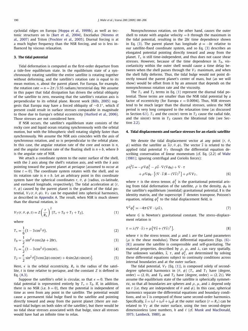
Figs. 1a and 1b show how the real and imaginary parts of theLove numbers vary with Δ. Notice that the real parts of the Lovenumbers are about the same for all values of Δ, and the imaginaryparts are always small. Thus the shell’s tidal bulge is still closelyaligned with the satellite–planet vector. The shell, in effect, stillmostly just rides up and down on the underlying ocean during itsnonsynchronous rotation. Its tidal displacement field is determinedalmost entirely by the shape of the ocean surface, and has littledependence on the shell’s rheological properties.

The shell’s rheology does have a significant impact on the shearstresses caused by that displacement field. Viscoelasticity in theshell can cause the shear stresses to be offset from the satellite–planet vector by up to ∼45◦ . For example, when Δ ≈ 1, μ and α inEqs. (32)–(36) have real and imaginary parts that are of the sameorder, and so they cause β1 and the other complex coefficients tohave significant imaginary parts even though (for a thin shell) theLove numbers h and � are almost real. (Figs. 1c and 1d show howthe real and imaginary parts of μ and λ vary with Δ.)

A perhaps counterintuitive result is that the stress pattern endsup being shifted in the direction opposite of the shell’s rotation,rather than in the same direction. This can be seen by noting thatthe real and imaginary parts of Eqs. (32)–(36) have the same sign,for h and � real. The stress pattern shifts in this direction be-cause Maxwell viscoelasticity causes the maximum displacementto occur after the maximum stress. Thus since the ocean-imposeddisplacement field is oriented toward the parent planet, the stresspattern is shifted in the direction the shell has rotated from. Onceagain, because the core is synchronously rotating, the forcing isconstant at every point in the core and so the core still respondsas though it were a fluid.

7. Numerical method, and a complication due to the core

For our numerical calculations we consider a satellite composedof four homogeneous compressible layers: a rocky core, an overly-ing fluid ocean, and a viscoelastic outer icy shell with a stiff upperlayer (representing a conductive stagnant lid) and a low-viscositybasal layer (representing a possible convective region).

We recognize that the very cold surface layer of the ice shellwill behave as a brittle-plastic material (e.g., Dombard and McK-innon, 2006) rather than viscously even on very long timescales.Whatever effect this near-surface layer has on the surface stressesis thus not accounted for in this model. However, if the fracturedlayer of the satellite extends to depths at which viscoelastic de-formation occurs on the timescale of NSR, then our model shouldprovide an accurate representation of the stresses at that depth.

In this example we choose the ice shell to be thin compared tothe satellite’s radius, but this is not a requirement of the method;it can be applied equally well to a satellite with a thick outershell, or even to a satellite with no liquid ocean at all. We de-termine the diurnal and NSR tidal solutions by solving the equa-tions of motion for a stratified, compressible, and self-gravitatingbody (Eqs. (6)–(8)). Our numerical method is based on standard


Fig. 1. The complex Love numbers h2 (a) and �2 (b). The dashed curves are calculations in which the silicate core has a nearly fluid response, appropriate to NSR (seeSection 7). The solid curves indicate a core having a nearly rigid response, appropriate to the diurnal forcing. Imaginary parts are thin curves, tied to the right axes; realparts are thick curves, tied to the left axes. The upper shell’s complex Lamé parameters λ (c) and μ (d). Thick dashed curves correspond to real parts and thin solid curvesare the imaginary parts. See Section 8.1 for discussion. All plots use the parameters listed in Table 1, and a range of forcing frequencies ω, represented here by the parameterΔ which represents the value of Δ in the upper layer.


Fig. 1. (continued)


algorithms used by geophysicists to compute tides on the Earth,and involves a modified version of the code used by Dahlen(1976) to compute terrestrial tides (see also Wahr et al., 2006;Rappaport et al., 2008). We have modified this code to includecomplex rheological parameters and complex solution scalars, sothat we can accommodate a Maxwell solid rheology. The diurnaland NSR solutions differ solely through the frequency-dependenceof the Lamé parameters, as shown in Eqs. (21)–(22). Once we havedetermined the complex Love numbers, h and �, they are used asdescribed in Section 5 to find the surface stresses.

In the formulation of the model described above, we assumethe coordinate system is attached to the icy shell and so ro-tates with it. The equations of motion (Eqs. (6)–(8)) depend onthe assumption that all displacements are small as seen in thiscoordinate system. These are reasonable assumptions for the di-urnal tides. However, in the case of NSR it is only the icy shellthat rotates nonsynchronously; the rocky core likely remains syn-chronously locked to the satellite’s orbital motion (Greenberg andWeidenschilling, 1984). From the perspective of points in the icyshell, which is the region of most interest to this study, the ex-ternal gravity field changes partly because the shell is rotatingthrough the parent planet’s gravity field, and partly because theshell is rotating through the gravity field caused by the underlyingcore. At points within the rocky core, on the other hand, the grav-ity field never changes, and so as described in Section 6, the corealways responds to the NSR tidal forcing as though it were a fluid.

To obtain an adequate representation of the shape of the coreand its effects on the icy shell, we set μ ≈ 0 in the rocky corewhen solving for the NSR tides. This eliminates shear stresses inthe core, leading to much larger core tidal displacements. This inturn significantly increases the displacements and shear stresses inthe icy shell, since then the gravity field from the core’s tidal bulgecan be a much larger fraction of the direct gravity field from theparent planet. On Europa for example, setting μ ≈ 0 in the corecan increase the displacements and shear stresses in the icy shellby up to 70%. This difference in the assumed behavior of the coreunder the diurnal and NSR forcings is why there are two sets ofeach of the Love numbers displayed in Figs. 1a and 1b.

8. Results

Our formulation of the equations of motion and the resultingstresses describes the effects of viscoelasticity in terms of the pa-rameter Δ, which is proportional to the ratio between the forcingperiod and the Maxwell relaxation time of the ice. Because theshell we are considering has two viscoelastic layers with differentviscosities, it will also have two values of Δ for a given forcingperiod. The resulting stresses at the outer surface (Eqs. (29)–(31))depend on those values in two ways:

(i) they depend on the Δ values of each ice layer through theLove numbers h and �; and

(ii) they depend on Δ of the upper icy layer only, through β1, γ1,β2, γ2, and Γ .

Item (i) represents the effects of viscoelasticity on the surface dis-placements, whereas (ii) describes how those displacements trans-late into stresses within a viscoelastic medium (with the propertiesof the upper ice layer). The dependence (i) is weak so long as thereis an underlying ocean and the ice shell is thin, as we are assum-ing in this application. Δ does have a large relative effect on theimaginary parts of the Love numbers, but the imaginary parts areonly a small fraction of the real parts. The tidal response in thiscase is mostly determined by the ocean, and so the Love numbersare only weakly dependent on the properties of the ice shell (seeMoore and Schubert, 2000; Wu et al., 2001; Wahr et al., 2006;

Rappaport et al., 2008). Thus, the primary influence of viscous ef-fects comes through (ii).

8.1. Love numbers

The effects of viscoelasticity on the real and imaginary parts ofthe Love numbers are shown in Figs. 1a and 1b, for values of Δ

(at the outer surface) spanning nine orders of magnitude. Valuesof Δ � 1 indicate a forcing period short enough that the shearstresses do not have time to relax during a forcing cycle, and sothe material behaves nearly elastically. Values of Δ � 1 imply along enough forcing period that the stresses have time to almostcompletely relax, allowing the material to behave almost as an in-viscid fluid.

The results shown in these figures are computed using the up-per and lower viscosity values ηupper and ηlower shown in Table 1,and varying the forcing period. The elastic value of μ, given in Ta-ble 1, is assumed to be the same in each layer. Thus, the results arecomputed assuming the values of Δ in the lower and upper lay-ers are related by a factor of Δlower/Δupper = ηupper/ηlower = 105.We would have obtained the same results if we had fixed the forc-ing period and varied the viscosities of the layers in tandem (i.e.maintaining ηupper/ηlower = 105).

Results are shown both for the diurnal tides, where the pe-riod is well known but the viscosity is not, and for the NSR tides,where neither the period nor the viscosity is known. The differ-ence between the diurnal and NSR results at any given value of Δ

is because in the NSR case we assume the silicate core behaves asa fluid, and in the diurnal case we assume it behaves elastically.As described in Section 7, this causes the NSR Love numbers to beabout 70% larger than the diurnal Love numbers for a fixed valueof Δ.

Figs. 1a and 1b show that the real parts of the Love numbers(thick lines, tied to left axes) are one to two orders of magnitudelarger than the imaginary parts (thin lines, right axes) no matterwhat value is assumed for Δ. This is because the icy lithosphere isthin and so has only a small impact on the surface displacementsregardless of whether it is viscoelastic or not. For the same rea-son, the real parts of the Love numbers vary by only ∼10% overthis entire range of Δ. This is important because the viscosity pro-file beneath the very outermost ice layer can perturb the surfacestresses only through its effects on the Love numbers, and the fig-ures show that those effects are likely to be no larger than ∼10%.Thus there is little additional accuracy to be gained by including amore complicated internal viscosity structure in the shell.

Figs. 1a and 1b also show dips in the values of the imaginaryparts of the Love numbers when Δ ≈ 1 and ≈ 10−5, with associ-ated step function increases in the real parts. The Δ ≈ 1 featuresreflect the transition from elastic-like to fluid-like behavior in theouter shell, as Δ transitions between <1 and >1. These featuresresult from similar behavior in the imaginary and real parts of μand λ of the outer shell evident in Figs. 1c and 1d. The featuresat Δ ≈ 10−5 are due to a similar elastic-to-fluid transition in thelower ice layer: a value of Δ = 10−5 in the upper layer impliesΔ = 1 in the lower layer because we have chosen to fix the ratioηupper/ηlower = 105.

There are also dips in the imaginary parts of the Love numbersat Δ ≈ 300, and corresponding step functions in the real parts.These features, which are far more prominent for the Love number� than for h, represent the effects of an additional relaxation modeof the system, a mode with a relaxation time that is considerablylonger than the Maxwell times of the ice layers. This situation isanalogous to the post-glacial-rebound process on the Earth. Vis-coelastic models of the Earth exhibit a large suite of relaxationmodes. Some directly correspond to Maxwell times. Others, re-ferred to as buoyancy modes, have longer periods and involve


radial displacements of density discontinuities. The Δ ≈ 300 modeevident in Figs. 1a and 1b corresponds to the viscoelastic modeusually referred to as C0 in the post-glacial-rebound literature, as-sociated with the relaxation of the Earth’s core-mantle boundary(e.g., Peltier, 1985). When the ocean/shell boundary is displacedfrom an equipotential surface, there is a gravitational (buoyancy)force that acts to restore it. This force is opposed by viscous re-sistance within the shell. Although this contribution to the vis-coelastic Love numbers is interesting from a dynamical viewpoint,its impact on the surface stresses is minimal because the Lovenumbers play only a secondary role in determining the viscoelas-tic contributions to the surface stresses. However, it does causethe maximum phase shift to slightly exceed 45◦ when Δ � 1, ascan be seen in Fig. 2a for Europa. Reducing the density contrastbetween the ice and the ocean reduces the buoyancy force, andincreases the timescale on which these forces have an effect, push-ing both the large dip in the imaginary part of �, and the increasein phase shift to values greater than 45◦ , out to larger Δ values.

8.2. The direct effects of the outer layer’s viscosity

Viscous effects influence the surface stresses most through theLamé parameters μ and λ of the upper shell, and their impact onthe parameters β1, γ1, β2, γ2, and Γ (Eqs. (32)–(36)). The surfacestress components (Eqs. (29)–(31)) are proportional to those lastfive parameters, and each of those parameters is proportional toμ of the outer surface. All except Γ also depend on λ, but thatdependence is not very strong. Figs. 1c and 1d show the Lamé pa-rameters as functions of Δ. Over the range of Δ considered here, μvaries enormously (from zero to 3.5 × 109 Pa) but λ varies by only∼30% (from ∼7 to ∼9 × 109 Pa). This variability, combined withthe direct influence of μ on all of the parameters listed above, im-plies that the Δ dependence of μ will strongly and directly impactthe surface stresses.

Note from Eq. (24) that Im(μ)/Re(μ) = Δ. Thus when Δ � 1the imaginary part is small relative to the real part, and whenΔ � 1 it is large (though both the real and imaginary parts vanishas Δ → ∞). When the real and imaginary parts are of compa-rable magnitude (i.e. 0.1 < Δ < 10), μ departs significantly fromeither the fluid or elastic limits. All of these characteristics of μget passed through directly to the stress components. The value ofΔ at the outer surface thus becomes critical in determining thesurface stresses.

For the diurnal tides, assuming a plausible value for the vis-cosity of cold surface ice of 1022 Pa s (Table 1), Δ in the upperlayer is roughly 2 × 10−8, which means the effects of viscoelastic-ity can be safely ignored. The outer surface viscosity would haveto be as small as 2 × 1015 Pa s for Δ to be as large as 0.1, which isroughly when viscous effects start to become important. A viscos-ity of 2×1015 Pa s may be reasonable for the warm lower ice layer,but as described above, the lower layer Δ has only a minimal im-pact on the surface stresses, no matter its value. The implicationis that viscoelastic effects are not likely to have a significant effecton the diurnal tidal stresses.

For the NSR tides (again assuming the outer layer viscosity is1022 Pa s), if the NSR period is between 1.2 × 105 and 1.2 × 107 yr,then Δ is in the range 0.1 < Δ < 10 where viscoelastic effects areimportant and are very sensitive to Δ. If the NSR period is sig-nificantly longer than 1.2 × 107 yr, then Δ � 1, and the surfacestresses are small: they decay away almost as quickly as the forc-ing can create them.

However, even relatively small NSR stresses can overwhelm thediurnal stresses. The diurnal tides arise because of the orbital ec-centricity ε , and cause displacements that are ε (= 0.0094 forEuropa) times as large as the NSR displacements. Thus, if the icelayer was elastic, the diurnal stresses would similarly be a factor

of ε times smaller than the NSR stresses. Viscoelasticity reducesthe NSR stress magnitudes as Δ increases (i.e. as the NSR pe-riod gets longer). For Δ � 1, the parameters β1, γ1, β2, γ2, andΓ in Eqs. (32)–(36) become approximately inversely proportionalto Δ. The elastic case is given by those same expressions, but withΔ = 0. Thus, in order for the amplitudes of the NSR stresses to bereduced to where they are comparable or smaller than the diur-nal amplitudes, Δ has to be on the order of 1/ε or larger (∼100for Europa). For an outer layer viscosity of 1022 Pa s, an NSR pe-riod of ∼1.2 × 108 yr or longer is required for diurnal stresses todominate NSR stresses.

8.3. Stress patterns and phase shifts

The value of Δ is critical for determining not only the mag-nitude of the surface stresses, but also how those stresses aredistributed over the surface of the satellite. The smaller the valueof Δ, the closer the shell’s response is to being elastic, and so thecloser the stresses are to being oriented symmetrically about theplanet–satellite vector — a state we will refer to as having zerophase shift.

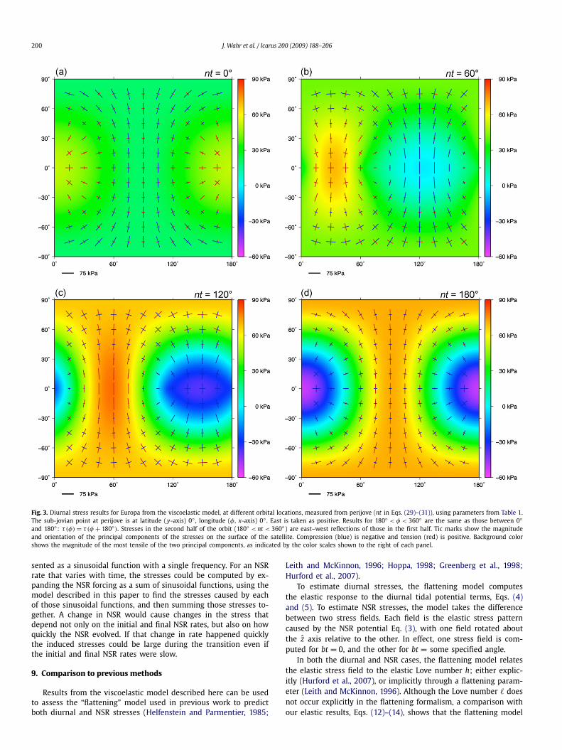
For the diurnal tides, Δ is so small that the resulting stressesare virtually elastic (see above). If the default viscosity values givenin Table 1 are altered such that the entire shell has the high vis-cosity of the surface (1022 Pa s), the amplitude of the diurnal com-ponent of the stresses changes by less than 0.1%. If the entire lowviscosity portion of the shell is replaced with ocean, leaving onlyan 8 km thick high-viscosity upper shell, the difference in the am-plitude of the diurnal component of the stresses is ∼3%. Maps ofthe diurnal stresses at different points in the orbit (i.e. at differentvalues of nt in Eqs. (29)–(31)) are shown in Fig. 3. In these plots,the sub-jovian point at perijove is at latitude (y-axis) 0◦ , longitude(x-axis) 0◦ .

For the NSR tides the value of the period is unknown. Boththe amplitude and the phase shift of the stresses depend on thatperiod, mostly through the direct dependence on Δ of the outersurface. The parameters β1, γ1, β2, γ2, and Γ (Eqs. (32)–(36))are proportional to μ, and μ depends on Δ through (24). Thus,the right-hand sides of Eqs. (32)–(36) show that when Δ � 1 theparameters β1, γ1, β2, γ2, and Γ are nearly real and are well ap-proximated by their elastic values (since h and � are nearly equalto their elastic values).

When Δ � 1, those five parameters have small amplitudes,but their imaginary parts are a factor of Δ larger than their realparts (for example, 1/(1 − iΔ) = (1 − iΔ)/(1 + Δ2), has real andimaginary parts of approximately Δ−2 and Δ−1 respectively, whenΔ � 1). This means that while τθθ is proportional to cos(2φ + 2bt)in the elastic limit, it is nearly proportional to sin(2φ + 2bt) in theΔ � 1 limit (see Eq. (38)). The factors of 2 in (2φ +2bt) mean thatthe spatial pattern of τθθ in the Δ � 1 limit is displaced from theelastic pattern by 45◦ . The same is true of the other stress compo-nents, τφφ and τφθ .

In general the patterns and amplitudes of the tidally inducedsurface stresses can be separated into 4 possible regimes. If theorbital eccentricity ε is small and the shell is thin, and assumingfor the case of Europa that the viscosity of the upper layer of theice is ηupper = 1022 Pa s, we find:

(a) Δ < 0.1. The NSR stress is nearly elastic, and so has a phaseshift of ∼0◦ . The NSR stress amplitude is a factor of ∼ε−1

times larger than the diurnal stress amplitude. For our nominalEuropa, this corresponds to an NSR period (Pnsr) of less than1.2 × 105 yr, and tensile NSR stresses of up to ∼3.2 MPa.

(b) 0.1 < Δ < 10. The NSR stress amplitude is still much largerthan that of the diurnal stress, but it varies rapidly throughthis range of Δ values (for Europa the NSR stress amplitude


Fig. 2. (a) NSR results from our viscoelastic model. Shown are the amplitude and phase shift of the maximum tensile stress at the outer surface of Europa as a function of Δ.The viscoelastic stress field experiences a phase shift >45◦ for large values of Δ because of the effect the ice shell’s buoyancy mode has on the imaginary part of the Lovenumber � for values of Δ ≈ 300 (see Fig. 1b, and discussion in Section 8.1). If the density contrast between the ice and the ocean is reduced, this upturn moves out to largervalues of Δ, as does that feature in �. (b) Similar to (a), with accumulated degrees of NSR for the flattening model (which we compare our model to in Section 9) alongthe x-axis. (c) Because the variables that the two models use to determine the phase shift and stress amplitudes are different (Δ for the viscoelastic model, accumulatedNSR for flattening), it is useful to compare the amplitudes as functions of the phase shift. The two curves are related by a nearly constant multiplier of ∼1.5, with theflattening model predicting larger amplitudes for an identical amount of phase shift. As the phase shift approaches 45◦ (implying small stress amplitudes), this multiplicativerelationship breaks down, with the amplitude of viscoelastic stresses eventually exceeding that of the flattening stresses.


Fig. 2. (continued)

decreases from ∼3.2 MPa to ∼500 kPa as Δ increases). Thephase shift varies from ∼0◦ at Δ = 0.1, to ∼45◦ at Δ = 10.For Europa this corresponds to 1.2 × 105 < Pnsr < 1.2 × 107 yr.

(c) 10 < Δ < ε−1 (≈100). The amplitude of the NSR stress hasrelaxed significantly, but is still as large or larger than that ofthe diurnal stress. The phase shift of the NSR stress patternis ∼45◦ . For Europa this corresponds to 1.2 × 107 < Pnsr <

1.2 × 108 yr, and results in the maximum tensile stress beingreduced from ∼500 kPa to ∼50 kPa as Δ increases throughthis range of values.

(d) Δ > ε−1 (≈100). The amplitude of the NSR stress is smallerthan that of the diurnal stress, becoming much smaller asΔ → ∞. The phase shift of the NSR stresses remains constantat ∼45◦ . However, for Δ � ε−1 this becomes irrelevant af-ter combining the NSR and diurnal stresses, because the NSRstress is overwhelmed by the diurnal stress. For Europa thiscorresponds to Pnsr > 1.2 × 108 yr.

These points are illustrated in Fig. 4, which shows NSR stressesfor different values of Δ. The maps show the stress results(Eqs. (38)–(40)) evaluated at time t = 0. At any time t , NSR wouldcause the sub-jovian point at be at longitude φ = −bt relative tothe Europan surface. Thus, these maps can also be interpreted asshowing the surface stresses at any time, relative to a sub-jovianpoint at latitude (y-axis) 0◦ and longitude (x-axis) 0◦ .

In the case of Europa, it is not yet possible to determine whichof the above regimes is appropriate. All four are possible given thecurrent uncertainty in the NSR period and the range of plausiblenear-surface ice viscosities.

8.4. Geological implications of viscoelasticity

Attempts have been made to correlate lineaments on Europawith the NSR stress field by translating them longitudinally (Hoppa

et al., 2001; Kattenhorn, 2002; Hurford et al., 2007; Figueredo andGreeley, 2000). The amount of translation required to get a good fitbetween a lineament and the stress field has been used as a proxyfor the time elapsed since formation. The underlying assumptionis that they formed at one longitude and, as the shell underwentNSR, they came to be located at another. This is only straightfor-ward if the stress field is fixed with respect to the planet–satellitevector and has a known phase shift (previously assumed to be∼45◦). Because Δ can affect the phase shift of the NSR stresses,the apparent longitude of formation of a lineament will also de-pend on Δ. If Δ is constant through time, this could introduce aconstant translation of up to 45◦ to the lineaments whose shapesare determined by the NSR stress field. But their apparent longi-tudes of formation could still potentially be used as a proxy fortheir relative times of formation. However, if we allow that Δ mayhave changed through time (Nimmo et al., 2006), it becomes dif-ficult to infer even a relative time of formation, since differentlineaments could have formed under different NSR stress regimeshaving different phase shifts.

Moreover, a variable Δ could allow the tidal stresses to tran-sition between being dominated by diurnal and NSR tides. Thiscould explain why on Europa we see both cycloidal lineaments (sofar best explained by the diurnal tides) and the long arcuate globallineaments (so far best explained by the NSR tides). If a changein Δ reflects a change in the rate of NSR, it could be that theglobal lineaments were formed during a period of rapid rotation inwhich the shell responded elastically to the NSR tide; and the cy-cloidal lineaments during a period of slow shell rotation, in whichthe NSR stresses were able to relax viscously, leaving the diurnaltide to dominate. Alternatively, a change in ice shell viscosity, e.g.through an episode of increased tidal heating or intense convec-tion, could produce a similar change in Δ over time.

The model described here assumes the rate of NSR is constant.It assumes the time-dependence of the NSR forcing can be repre-


Fig. 3. Diurnal stress results for Europa from the viscoelastic model, at different orbital locations, measured from perijove (nt in Eqs. (29)–(31)), using parameters from Table 1.The sub-jovian point at perijove is at latitude (y-axis) 0◦ , longitude (φ , x-axis) 0◦ . East is taken as positive. Results for 180◦ < φ < 360◦ are the same as those between 0◦and 180◦: τ (φ) = τ (φ + 180◦). Stresses in the second half of the orbit (180◦ < nt < 360◦) are east–west reflections of those in the first half. Tic marks show the magnitudeand orientation of the principal components of the stresses on the surface of the satellite. Compression (blue) is negative and tension (red) is positive. Background colorshows the magnitude of the most tensile of the two principal components, as indicated by the color scales shown to the right of each panel.

sented as a sinusoidal function with a single frequency. For an NSRrate that varies with time, the stresses could be computed by ex-panding the NSR forcing as a sum of sinusoidal functions, using themodel described in this paper to find the stresses caused by eachof those sinusoidal functions, and then summing those stresses to-gether. A change in NSR would cause changes in the stress thatdepend not only on the initial and final NSR rates, but also on howquickly the NSR evolved. If that change in rate happened quicklythe induced stresses could be large during the transition even ifthe initial and final NSR rates were slow.

9. Comparison to previous methods

Results from the viscoelastic model described here can be usedto assess the “flattening” model used in previous work to predictboth diurnal and NSR stresses (Helfenstein and Parmentier, 1985;

Leith and McKinnon, 1996; Hoppa, 1998; Greenberg et al., 1998;Hurford et al., 2007).

To estimate diurnal stresses, the flattening model computesthe elastic response to the diurnal tidal potential terms, Eqs. (4)and (5). To estimate NSR stresses, the model takes the differencebetween two stress fields. Each field is the elastic stress patterncaused by the NSR potential Eq. (3), with one field rotated aboutthe z axis relative to the other. In effect, one stress field is com-puted for bt = 0, and the other for bt = some specified angle.

In both the diurnal and NSR cases, the flattening model relatesthe elastic stress field to the elastic Love number h; either explic-itly (Hurford et al., 2007), or implicitly through a flattening param-eter (Leith and McKinnon, 1996). Although the Love number � doesnot occur explicitly in the flattening formalism, a comparison withour elastic results, Eqs. (12)–(14), shows that the flattening model


Fig. 4. NSR stress results from the viscoelastic model for Europa at different values of Δ. Plots are similar to those in Fig. 3. The sub-jovian point is at latitude = longitude= 0◦ . This pattern is repeated for φ > 180◦: τ (φ) = τ (φ + 180◦). The tic mark length and color scales indicating stress magnitudes vary among the four panels. Results arecomputed using the input parameters shown in Table 1, with the exception of the orbital eccentricity ε , which has been set to zero to exclude contributions from diurnalstresses. (a) Δ = 0.1, corresponding to nearly elastic stresses. The stress field is close to symmetric about the planet–satellite vector (which passes through 0◦ and 180◦longitude), though a small westward shift in the stresses is evident. (b) Δ = 1. The magnitudes of the stresses have been reduced slightly by relaxation, but the westwardphase shift has increased significantly. (c) Δ = 10. The NSR stresses have largely relaxed away, though they are still significantly larger than the diurnal stresses pictured inFig. 3. Here the phase shift is nearly complete, with the region of greatest tensile stress close to its maximum separation from the planet–satellite vector. (d) Δ = 100 (∼ε−1

for Europa). The overall NSR stress pattern is persistent, but the magnitudes are significantly smaller than those in Fig. 3. See Section 8.3 for further discussion.

implicitly assumes � = h/4, a result that is in good agreement withthe elastic Love number results found here (see Figs. 1a and 1b inthe Δ → 0 limit).

Figs. 5a and 5b compare our diurnal stress results with thoseof the flattening model applied to a similar satellite. Both sets ofresults were computed for a time corresponding to 225◦ after per-ijove (i.e. nt = 225◦ in Eqs. (29)–(31)). The two methods predictsimilar overall patterns. Amplitude differences are on the order ofonly 7%, and presumably reflect differences between the interiormodels used.

The situation is more complicated for the NSR stresses. Theflattening method’s representation of those stresses as the differ-

ence between two elastic stress fields is somewhat ad hoc, and itsrelationship to the viscoelastic properties of the shell is not imme-diately obvious. Fig. 2 can be used to empirically understand thatrelationship.

Fig. 2a shows the largest tensile stress magnitude and the phaseshift for the viscoelastic NSR model, as a function of Δ in the up-per ice layer. The phase shift is defined here as the number ofdegrees of longitude separating the greatest tensile stress and theplanet–satellite vector. For an elastic satellite the phase shift = 0◦ .Large values of Δ, corresponding to slow NSR rates and/or shortviscous relaxation times, lead to phase shifts of 45◦ and smallstress amplitudes.


Fig. 5. Stresses computed using the “flattening” method (left) compared to those from our viscoelastic model (right) for a Europa-like satellite with similar physical properties.Table 4 lists the input parameters adopted for the flattening calculations (T. Hurford, personal communication, 2006). These parameters, excluding the real valued Lovenumbers, have also been adopted for the viscoelastic calculations. Because the viscoelastic model requires more information about the internal structure of the satellitein order to calculate the frequency-dependent Love numbers, those parameters in Table 1 not listed in Table 4 have been adopted in (b) and (d). (a) Flattening and (b)viscoelastic results for diurnal stresses at 225◦ after perijove (i.e. nt = 225◦ in Eqs. (29)–(31)). (c) NSR stresses from the flattening method with 1◦ of accumulated NSR,compared to those calculated by the viscoelastic model (d) with Δ = 56, at which point the two models each have a phase shift of 44.5◦ . See Section 9 for discussion.

Table 4Flattening model parameters (Figs. 2 and 5).

Parameter Symbol Value

Elastic Love number h 1.2753Elastic Love number � 0.31882 (≡ h

4 )

Mass of Europa ME 4.80 × 1022 kgMass of Jupiter Mp 1.8986 × 1027 kgRadius of Europa Rs 1.561 × 106 mEuropa’s orbital semi-major axis a 6.709 × 108 mEccentricity of orbit ε 0.01Bulk modulus of ice (= λice + 2

3 μice) κice 9.1764 × 109 PaShear modulus of ice μice 3.5187 × 109 Pa

Fig. 2b shows the same quantities for the flattening model, as afunction of the rotation angle between the two elastic stress pat-

terns (the “accumulated degrees of NSR,” which in the flatteningmodel is the parameter that describes how much stress is allowedto build up in the shell, similar to our Δ). Small values of the ro-tation angle result in large phase shifts and small amplitudes. Thiscan be understood by considering, for example, τθθ . The elastic re-sult (Eq. (12)) has a longitudinal dependence of cos(2φ + 2bt). Thedifference between this cosine and the same cosine when φ hasbeen rotated by the angle δ, is cos(2φ +2bt)−cos(2φ +2δ+2bt) ≈(when δ is small) δ sin(2φ + 2bt). Thus, the difference decreases inamplitude as δ → 0, and lags cos(2φ + 2bt) by 45◦ in φ. The dif-ference between these cosines has an increasing amplitude and adecreasing phase shift as δ increases, consistent with the resultsshown in Fig. 2b.


Fig. 2c compares our viscoelastic results with the flattening re-sults, by plotting the maximum stress as a function of the phaseshift. The general shapes of the viscoelastic and flattening curvesare similar. Though for a given phase shift the flattening modeltends to overestimate the maximum stress amplitude by a factorof about 1.5. Alternatively, for a given maximum stress the flat-tening model predicts a larger phase shift. The results thus showthat the viscoelastic and flattening models predict different rela-tionships between the magnitude of the NSR stresses and theirlocation on the surface of the satellite. Either the phase shift orthe magnitude of the NSR stresses can match, but not both simul-taneously. Note that had we not allowed shear stresses to relaxin the synchronously rotating core by using a low value of μcore inthe NSR Love number calculations, as discussed in Section 7 above,the real parts of the NSR Love numbers would have been similar tothe diurnal values (see Figs. 1a and 1b, and Tables 2 and 3), result-ing in the viscoelastic stresses being ∼35% smaller, and increasingthe difference from the flattening model even more.

To compare spatial stress patterns for the two different modelsof NSR stresses, we need to match up values of Δ in the viscoelas-tic model with corresponding values of accumulated NSR in theflattening model. The results shown in Figs. 2a and 2b indicatethat small values of accumulated NSR correspond to large valesof Δ (i.e. to long NSR periods and/or small viscosities). For ev-ery value of accumulated NSR in the flattening model we find thecorresponding value of Δ in the viscoelastic model such that thetwo models give identical phase shifts for the maximum tensilestress. Because of the linear relationship between phase shift andthe amount of accumulated NSR evident in Fig. 2b, we expect 1◦of NSR to result in a phase lag of 44.5◦ (= 45◦ − (0.5 × NSR)).For the parameters used in these calculations, this corresponds toΔ = 56. The comparison can be seen in Figs. 5c and 5d. The spatialpatterns are in good agreement. The amplitudes of the flatteningstresses are larger than the amplitudes of the viscoelastic stresses,but only by ∼20% rather than the ∼50% that might be expectedfrom Fig. 2c. This is because Figs. 5c and 5d consider a phase shiftclose to 45◦ , which is where the flattening model has usually beenapplied in the past. Fig. 2c shows that as the phase shift gets closeto 45◦ the amplitude of the viscoelastic stresses approaches andeventually even exceeds that of the flattening stresses, though bothare small at large values of Δ. This is partly due to the buoyancymode described at the end of Section 8.1, which begins to influ-ence the surface stresses when Δ exceeds ∼10 (see Figs. 1a, 1b,and 2a). The flattening stresses reach zero amplitude when thephase shift is 45◦ , but the viscoelastic stresses maintain an am-plitude of at least a few kPa until the phase shift is close to 50◦ ,and vanish only as Δ → ∞.

10. Summary and future work

We have developed and implemented a method of calculatingthe tidally induced surface stresses of a radially stratified satellitewith a Maxwell viscoelastic shell of arbitrary thickness overlyingan inviscid ocean and a silicate core, derived directly from thetime-varying gravitational potential experienced by the satellite.All regions of the satellite are compressible and self-gravitating.The formalism could easily be extended to also include viscoelas-ticity within the silicate core, though we have chosen not to do sohere. The results could also readily be extended to find the stressfield at any depth within the shell, by using output from the nu-merical Love number code at subsurface depths.

We have applied this model to radial and librational diurnaltides caused by the eccentricity of the satellite’s orbit, and to tidesthat would be caused by faster than synchronous rotation of afloating shell. In both these cases we assumed the satellite’s orbithas zero obliquity, so that the orbital motion is in the satellite’s

equatorial plane, and that the NSR motion occurs in that sameplane.

Viscoelastic effects are incorporated through the use of frequen-cy-dependent, complex-valued Lamé parameters and Love num-bers. The inclusion of viscous relaxation has significant implica-tions for the NSR stress environment at the satellite’s surface, bothreducing the magnitude of stresses due to long period forcings,and inducing a phase shift that translates the NSR stress field inthe opposite direction of shell rotation. The importance of theseeffects depends on the ratio of the NSR period to the viscous re-laxation time of the satellite’s outer surface, a ratio described hereby the parameter Δ. If Δ � 10, NSR stresses are much larger thandiurnal stresses, and are very similar to the elastic limit with a∼0◦ phase shift. If Δ � 100, the NSR stresses will have a phaseshift of ∼45◦ , but their amplitude will be smaller than the diurnalstresses. The effects of viscoelasticity on the diurnal stresses areinsignificant for any plausible value of outer surface viscosity.

Because Δ affects the phase shift of the stress field, the appar-ent longitude of formation of a lineament will also depend on Δ. Ifwe accept the possibility that Δ changes through time, this makesit more difficult to use a lineament’s apparent longitude of forma-tion as a proxy for its time of formation, even relative to otherlineaments, since they may have formed under NSR stress regimeswith different phase shifts.

If we think the linear features observed on the surface of anicy satellite are tidally induced or influenced fractures, it must fol-low that the surface stresses sometimes exceed the strength of theicy lithosphere. This implies that localized stress release due tobrittle failure plays a role in defining the surface stress environ-ment (Smith-Konter and Pappalardo, 2008). It would be beneficialto incorporate the formation of brittle fractures and the resultingchanges in the stress field into the viscoelastic model (cf. King etal., 1994). However, that modeling is inherently numerical, requir-ing localized adjustment of the stresses as each crack forms andaffects the formation of subsequent fractures in the region. Thus,the stresses of our model are those one would expect to find onthe surface of a viscoelastic shell stronger than the greatest cal-culated stress. In this paper we have applied this model to thestresses experienced by a shell in steady state with a constantrotation rate, but there are many other possible scenarios for re-orientation of a decoupled shell that are not well represented bya steady-state solution. A time-variable NSR rate can easily be ac-commodated using the formalism described here, while calculatingthe time evolution of stresses due to episodic polar wander will re-quire enhancements to the model.

11. Sharing the model with the community

Other researchers are encouraged to create their own imple-mentation of the model described in this paper. For those whoprefer to use, verify, or build upon our implementation of themodel, we are providing access to the code under a public licenseat: http://code.google.com/p/satstress.

We are also providing a web-based interface to the model at:http://icymoons.com/satstress where users may input model pa-rameters, and perform regularly gridded calculations like thoseused to generate the figures presented in this paper.

An important benefit of hosting the model on the web is thatindividual model runs can be archived automatically for later ref-erence. For example, Table 5 contains the unique model run IDsof the SatStress calculations that went into making Figs. 3–5. Withone of these IDs a user can view all the model inputs and outputspertaining to the run. They can also use any run ID as the basisof a new model run. This centralized recordkeeping makes it eas-ier to track and compare model inputs and outputs without having

http://code.google.com/p/satstress

http://icymoons.com/satstress


Table 5SatStress run IDs for figures in this paper.

Fig. Run ID

3a 20080121182229_4795536555ce93b 20080121183751_479556ff3edfa3c 20080121183841_4795573178a183d 20080121183921_479557592a9dc4a 20080122145730_479674da20bc24b 20080122145857_47967531914834c 20080122150014_4796757e38a134d 20080122150135_479675cfe6ef05b 20080123194857_47980aa9b37a45d 20080123191023_4798019f7b218

to keep track of every parameter involved in a calculation, and wehope it will facilitate future collaboration.

Acknowledgments

We are grateful to Terry Hurford for providing us with numer-ical output from the “flattening” model equivalent to that used inplots from Greenberg et al. (1998), to Francis Nimmo for thought-ful discussions, and to Bridget Smith-Konter and Simon Katten-horn for beta-testing of our implementation. We thank Isamu Mat-suyama and an anonymous reviewer for helpful comments on themanuscript. Support for this work is provided by NASA PlanetaryGeology and Geophysics Grant NNG04GJ19G, and NASA Outer Plan-ets Research Program Grant NNG06GF44G, and the NASA Astrobi-ology Institute under Cooperative Agreement No. CAN-XX-OSS-02issued through the Office of Space Science.

Appendix A. Tidal potential

Let (r, θ , φ) be the spherical coordinates (r = radius, θ = co-latitude, φ = longitude) of a point in the satellite. The general formof the tidal potential at (r, θ , φ) caused by an external point mass(the parent planet), is given in Eq. (1) of Kaula (1964) (changingsome of the variable names):

V T (r, θ,φ) = Gm∗

a∗∞∑

l=2

(r

a∗

)l l∑m=0

(l − m)!(l + m)! (2 − δ0m)

× Plm(cos θ)∑p,q

Flmp(i∗

)Glpq(ε)

×[

cos(mφ)

{cossin

}l−m=even

l−m=odd

{(l − 2p)ω∗

+ (l − 2p + q)M∗ + m(Ω∗ − Θ∗)}

+ sin(mφ)

{sin

− cos

}l−m=even

l−m=odd

{(l − 2p)ω∗

+ (l − 2p + q)M∗ + m(Ω∗ − Θ∗)}]

, (A.1)

where the six Keplerian elements that describe the parent planet’sapparent motion are Ω∗ (longitude of the ascending node), M∗(mean anomaly), i∗ (inclination), a∗ (semi-major axis), ω∗ (argu-ment of pericenter), and ε (eccentricity). Other variables are: Θ∗ isthe sidereal time of the reference meridian, m∗ is the mass of theplanet, G is Newton’s gravitational constant, the Plm(cos θ) are as-sociated Legendre functions, and the Flmp(i∗) and Glpq(ε) are poly-nomials given in Tables 2 and 3 of Kaula (1964). For most satellitesof interest r/a∗ � 1. For Europa, for example, r/a � 0.0023. Thus,as is usual, we keep only l = 2 terms in (A.1). We set i∗ = 0 (sincewe are assuming the satellite’s obliquity vanishes), which causesthe only non-zero F2mp(i∗) to be F220 = 3, and F201 = −1/2. We

assume the eccentricity is small (ε ∼ 0.0094 for Europa), and ex-pand Glpq(ε) in powers of ε keeping terms only up to first order.We set M∗ = nt (which is exact for Keplerian orbits), and assumeΘ∗ = (n + b)t (Θ∗ represents the angular displacement betweenthe vector to the planet and the x-axis in our satellite-fixed coor-dinate system). By choosing M∗ = nt , we are defining t = 0 as thetime of periapse. Because the inclination vanishes, there is no dis-tinction between Ω∗ and ω∗ , and only the sum (Ω∗ +ω∗) appearsin the final solution. We set this sum to zero, which, together withour assumption that Θ∗ = 0 at t = 0, implies that not only is thesatellite at periapse at time t = 0, but its x-axis is pointing towardthe planet at that time. The longitude, φ, of a point in the satel-lite is defined as the angle eastward (i.e. counterclockwise as seenfrom above the rotation axis) from this x-axis. Using expressionsfor the Plm(cos θ) gives:

V T (r, θ,φ, t) = Z

(r

Rs

)2[1

6

(1 − 3 cos2 θ

) + 1

2sin2 θ cos(2φ + 2bt)

+ ε

2

(1 − 3 cos2 θ

)cos(nt)

+ ε

4sin2 θ

[7 cos

(2φ − (n − 2b)t

)− cos

(2φ + (n + 2b)t

)]], (A.2)

where

Z = 3Gm∗R2s

2a∗3, (A.3)

and Rs is the radius of the satellite.The last two terms on the right-hand side of Eq. (A.2) have

angular frequencies of (n−2b) and (n+2b), respectively. Because b(the rate of NSR) is much smaller than n (the mean motion; which,for a satellite in near-synchronous rotation, is about equal to thediurnal rotation rate), we can ignore b in both those frequencies.In that case, V T reduces to Eq. (1) in the main text, reproducedhere:

V T (r, θ,φ, t) = Z

(r

Rs

)2

[T∗ + T0 + T1 + T2], (A.4)

given that

T∗ = 1

6

(1 − 3 cos2 θ

), (A.5)

T0 = 1

2sin2 θ cos(2φ + 2bt), (A.6)

T1 = ε

2

(1 − 3 cos2 θ

)cos(nt), (A.7)

T2 = ε

2sin2 θ

[3 cos(2φ) cos(nt) + 4 sin(2φ) sin(nt)

]. (A.8)

Appendix B. Surface stresses for elastic satellites

The stress tensor associated with the tidal displacement vector,is given by Eq. (8) in the main text:

τ = λ(∇ · �s ) + μ[∇�s + (∇�s )T ]

. (B.1)

We use this relation, together with the surface displacement com-ponents first defined in Eqs. (9)–(11):

sr(r = Rs, θ,φ, t) =(

h

g

)V T

∣∣∣∣r=Rs

, (B.2)

sθ (r = Rs, θ,φ, t) =(

�

g

)∂V T

∂θ

∣∣∣∣r=Rs

, (B.3)

sφ(r = Rs, θ,φ, t) =(

�

g sin θ

)∂V T

∂φ

∣∣∣∣ (B.4)
r=Rs


and the tidal potential Eq. (1), to find τ at the outer surface asfollows.

As noted in Section 4, τrr = τθr = τφr = τrθ = τrφ = 0 at theouter surface. Writing [∇�s + (∇�s)T ] and ∇ · �s in spherical coordi-nates, as given by Eqs. (A139) and (A140) of Dahlen and Tromp(2001), we find that:

τrr = λ

Rs

[Rs∂r sr + 2sr + ∂θ sθ + sθ cot θ + ∂φ sφ

sin θ

]+ 2μ∂r sr = 0. (B.5)

This implies that at the outer surface (where τrr = 0):

∂r sr = −λ

Rs(λ + 2μ)

[2sr + ∂θ sθ + sθ cot θ + ∂φ sφ

sin θ

], (B.6)

so that (using Eq. (B.6) in Eq. (A140) of Dahlen and Tromp, 2001):

∇ · �s = 2μ

Rs(λ + 2μ)

[2sr + ∂θ sθ + sθ cot θ + ∂φ sφ

sin θ

]. (B.7)

The only non-zero stress components at the outer surface areτθθ , τθφ = τφθ and τφφ . Using the spherical components of [∇�s +(∇�s)T ] given by Eq. (A139) in Dahlen and Tromp (2001), and usingEq. (B.7) for ∇ · �s, gives:

τθθ = 2μ

Rs(λ + 2μ)

[(3λ + 2μ)sr + 2(λ + μ)∂θ sθ

+ λ

(∂φ sφ

sin θ+ sθ cot θ

)], (B.8)

τφφ = 2μ

Rs(λ + 2μ)

[(3λ + 2μ)sr + λ∂θ sθ

+ 2(λ + μ)

(∂φ sφ

sin θ+ sθ cot θ

)], (B.9)

τφθ = τθφ = μ

Rs

[∂θ sφ + ∂φ sθ

sin θ− sφ cot θ

]. (B.10)

At the outer surface, the displacements sr , sθ , and sφ can berelated to the tidal potential, V T |Rs , evaluated at the outer surface,using the Love numbers h and � as described in (B.2)–(B.4). Usingthose results in Eqs. (B.8)–(B.10), gives:

τθθ = 2μ

g Rs(λ + 2μ)

[h((3λ + 2μ)V T |Rs

)+ �

(λ

sin2 θ∂2φ V T |Rs + λ cot θ∂θ V T |Rs + 2(λ + μ)∂2

θ V T |Rs

)],

(B.11)

τφφ = 2μ

g Rs(λ + 2μ)

[h((3λ + 2μ)V T |Rs

)+ �

(2(λ + μ)

sin2 θ∂2φ V T |Rs + 2(λ + μ) cot θ ∂θ V T |Rs

+ λ∂2θ V T |Rs

)], (B.12)

τφθ = τθφ = 2μ�

g Rs sin θ

[∂2θφ V T |Rs − cot θ∂φ V T |Rs

]. (B.13)

Finally, using Eq. (1) to find V T |Rs gives the results shown inEqs. (12)–(14) of the main text:

τθθ = Z

2g Rs

[−1

3

(β1 + 3γ1 cos(2θ)

)+ (

β1 − γ1 cos(2θ))

cos(2φ + 2bt)

+ 3ε(β1 − γ1 cos(2θ)

)cos(nt) cos(2φ)

− ε(β1 + 3γ1 cos(2θ)

)cos(nt)

+ 4ε(β1 − γ1 cos(2θ)

)sin(nt) sin(2φ)

], (B.14)

τφφ = Z

2g Rs

[−1

3

(β2 + 3γ2 cos(2θ)

)+ (

β2 − γ2 cos(2θ))

cos(2φ + 2bt)

+ 3ε(β2 − γ2 cos(2θ)

)cos(nt) cos(2φ)

− ε(β2 + 3γ2 cos(2θ)

)cos(nt)

+ 4ε(β2 − γ2 cos(2θ)

)sin(nt) sin(2φ)

], (B.15)

τφθ = τθφ = 2�Zμ

g Rs

[− cos θ sin(2φ + 2bt) + 4ε sin(nt) cos θ cos(2φ)

− 3ε cos(nt) cos θ sin(2φ)]. (B.16)

References

Bart, G.D., Turtle, E.P., Jaeger, W.L., Keszthelyi, L.P., Greenberg, R., 2004. Ridges andtidal stress on Io. Icarus 169, 111–126.

Bills, B.G., 2005. Free and forced obliquities of the Galilean satellites of Jupiter.Icarus 175, 233–247.

Collins, G.C., Head, J.W., Pappalardo, R.T., 1998. Formation of Ganymede grooved ter-rain by sequential extensional episodes: Implications of Galileo observations forregional stratigraphy. Icarus 135, 345–359.

Croft, S.K., Soderblom, L.A., 1991. Geology of the uranian satellites. In: Bergstralh, J.T.,Miner, E.D., Matthews, M.S. (Eds.), Uranus. University of Arizona Press, Tucson,AZ, pp. 561–628.

Croft, S.K., Kargel, J.S., Moore, J.M., Schenk, P.M., Strom, R.G., 1995. Geology of Tri-ton. In: Cruikshank, D.P. (Ed.), Neptune and Triton. University of Arizona Press,Tucson, AZ, pp. 879–948.

Dahlen, F., 1976. The passive influence of the oceans upon the rotation of the Earth.Geophys. J. R. Astron. Soc. 46, 363–406.

Dahlen, F.A., Tromp, J., 2001. Theoretical Global Seismology. Princeton UniversityPress, Princeton, NJ.

Dobrovolskis, A.R., 1982. Internal stresses in Phobos and other triaxial bodies.Icarus 52, 136–148.

Dombard, A.J., McKinnon, W.B., 2006. Folding of Europa’s icy lithosphere: An anal-ysis of viscous-plastic buckling and subsequent topographic relaxation. J. Struct.Geol. 28, 2259–2269.

Figueredo, P.H., Greeley, R., 2000. Geologic mapping of the northern leading hemi-sphere of Europa from Galileo solid-state imaging data. J. Geophys. Res. 105,22629–22646.

Geissler, P.E., Greenberg, R., Hoppa, G., Helfenstein, P., McEwen, A., Pappalardo, R.,Tufts, R., Ockert-Bell, M., Sullivan, R., Greeley, R., Belton, M.J.S., Denk, T., Clark,B.E., Burns, J., Veverka, J., 1998. Evidence for non-synchronous rotation of Eu-ropa. Nature 391, 368–370.

Greeley, R.C., Chyba, C., Head, J.W., McCord, T., McKinnon, W.B., Pappalardo, R.T.,2004. Geology of Europa. In: Bagenal, F., Dowling, T.E., McKinnon, W.B. (Eds.),Jupiter: The Planet, Satellites and Magnetosphere. Cambridge University Press,New York, pp. 329–362.

Greenberg, R., Weidenschilling, S.J., 1984. How fast do Galilean satellites spin?Icarus 58, 186–196.

Greenberg, R., Geissler, P., Hoppa, G., Tufts, B.R., Durda, D.D., Pappalardo, R., Head,J.W., Greeley, R., Sullivan, R., Carr, M.H., 1998. Tectonic processes on Europa:Tidal stresses, mechanical response, and visible features. Icarus 135, 64–78.

Harada, Y., Kurita, K., 2007. Effect of non-synchronous rotation on surfacestress upon Europa: Constraints on surface rheology. Geophys. Res. Lett. 34,doi:10.1029/2007GL029554. L11204.

Helfenstein, P., Parmentier, E.M., 1983. Patterns of fracture and tidal stresses on Eu-ropa. Icarus 53, 415–430.

Helfenstein, P., Parmentier, E.M., 1985. Patterns of fracture and tidal stresses due tononsynchronous rotation—Implications for fracturing on Europa. Icarus 61, 175–184.

Hoppa, G.V., 1998. Europa: Effects of rotation and tides on tectonic processes. Doc-toral thesis, p. 227.

Hoppa, G.V., Tufts, B.R., Greenberg, R., Geissler, P., 1999a. Strike-slip faults on Eu-ropa: Global shear patterns driven by tidal stress. Icarus 141, 287–298.

Hoppa, G.V., Tufts, B.R., Greenberg, R., Geissler, P.E., 1999b. Formation of cycloidalfeatures on Europa. Science 285, 1899–1902.

Hoppa, G.V., Greenberg, R., Geissler, P., Tufts, B.R., Plassmann, J., Durda, D.D., 1999c.Rotation of Europa: Constraints from terminator and limb positions. Icarus 137,341–347.

Hoppa, G.V., Tufts, B.R., Greenberg, R., Hurford, T.A., O’Brien, D.P., Geissler, P.E., 2001.Europa’s rate of rotation derived from the tectonic sequence in the Astypalaearegion. Icarus 153, 208–213.

Hurford, T.A., Bills, B.G., Sarid, A.R., Greenberg, R., 2006. Unraveling Europa’s tectonichistory: Evidence for a finite obliquity? Lunar Planet. Sci. 37. Abstract 1303.

Hurford, T.A., Sarid, A.R., Greenberg, R., 2007. Cycloidal cracks on Europa: Improvedmodeling and non-synchronous rotation implications. Icarus 186, 218–233.

http://dx.doi.org/10.1029/2007GL029554


Kattenhorn, S.A., 2002. Nonsynchronous rotation evidence and fracture history inthe bright plains region, Europa. Icarus 157, 490–506.

Kaula, W.M., 1964. Tidal dissipation by solid friction and the resulting orbital evolu-tion. Rev. Geophys. 2, 661–685.

King, G.C.P., Stein, R.S., Lin, J., 1994. Static stress changes and the triggering of earth-quakes. Bull. Seismol. Soc. Am. 84, 935–953.

Lambeck, K., 1980. The Earth’s Variable Rotation: Geophysical Causes and Conse-quences. Cambridge University Press, Cambridge, England.

Leith, A.C., McKinnon, W.B., 1996. Is there evidence for polar wander on Europa?Icarus 120, 387–398.

McEwen, A.S., 1986. Tidal reorientation and the fracturing of Jupiter’s moon Europa.Nature 321, 49–51.

McEwen, A.S., Keszthelyi, L.P., Lopes, R., Schenk, P.M., Spencer, J.R., 2004. The litho-sphere and surface of Io. In: Bagenal, F., Dowling, T.E., McKinnon, W.B. (Eds.),Jupiter: The Planet, Satellites and Magnetosphere. Cambridge University Press,New York, pp. 307–328.

Melosh, H.J., 1975. Large impact craters and the Moon’s orientation. Earth Planet.Sci. Lett. 26, 353–360.

Melosh, H.J., 1977. Global tectonics of a despun planet. Icarus 31, 221–243.Melosh, H.J., 1980a. Tectonic patterns on a reoriented planet—Mars. Icarus 44, 745–

751.Melosh, H.J., 1980b. Tectonic patterns on a tidally distorted planet. Icarus 43, 334–

337.Meyer, J., Wisdom, J., 2007. Tidal heating in Enceladus. Icarus 188, 535–539.Moore, W.B., Schubert, G., 2000. The tidal response of Europa. Icarus 147, 317–

319.Munk, W., MacDonald, G., 1975. The Rotation of the Earth. Cambridge University

Press, Cambridge, England.Nimmo, F., Pappalardo, R.T., 2004. Furrow flexure and ancient heat flux on

Ganymede. Geophys. Res. Lett. 31, doi:10.1029/2004GL020763. L19701.Nimmo, F., Pappalardo, R.T., 2006. Diapir-induced reorientation of Saturn’s moon

Enceladus. Nature 441, 614–616.Nimmo, F., Thomas, P.C., Pappalardo, R.T., Moore, W.B., 2006. Inferring the state of

tidally-heated satellite ice shells from global shape measurements. Eos Trans.AGU 87.

Nimmo, F., Spencer, J.R., Pappalardo, R.T., Mullen, M.E., 2007. Shear heating as theorigin of the plumes and heat flux on Enceladus. Nature 447, 289–291.

Ojakangas, G.W., Stevenson, D.J., 1989. Thermal state of an ice shell on Europa.Icarus 81, 220–241.

Pappalardo, R.T., Collins, G.C., Head, J.W., Helfenstein, P., McCord, T., Moore, J.M.,Prockter, L.M., Schenk, P.M., Spencer, J.R., 2004. Geology of Ganymede. In: Bage-

nal, F., Dowling, T.E., McKinnon, W.B. (Eds.), Jupiter: The Planet, Satellites andMagnetosphere. Cambridge University Press, New York, pp. 363–396.

Peale, S.J., 1999. Origin and evolution of the natural satellites. Annu. Rev. Astron.Astrophys. 37, 533–602.

Peltier, W.R., 1974. The impulse response of a Maxwell Earth. Rev. Geophys. SpacePhys. 12, 649–669.

Peltier, W.R., 1985. The LAGEOS constraint on deep mantle viscosity: Result from anew normal mode method for the inversion of viscoelastic relaxation spectra. J.Geophys. Res. 90, 9411–9421.

Prockter, L.M., Pappalardo, R.T., Nimmo, F., 2005. A shear heating origin for ridgeson Triton. Geophys. Res. Lett. 32, doi:10.1029/2005GL022832. L14202.

Rappaport, N.J., Iess, L., Wahr, J.M., Lunine, J.I., Armstrong, J.W., Asmar, S.W., Tortora,P., Di Benedetto, M., Racioppa, P., 2008. Can Cassini detect a subsurface ocean inTitan from gravity measurements? Icarus 194, 711–720.

Schenk, P., Hargitai, H., Wilson, R., McEwen, A., Thomas, P., 2001. The mountainsof Io: Global and geological perspectives from Voyager and Galileo. J. Geophys.Res. 106 (E15), 33201–33222.

Schubert, G., Anderson, J.D., Spohn, T., McKinnon, W.B., 2004. Interior Composition,Structure and Dynamics of the Galilean Satellites. Cambridge University Press,New York, pp. 263–280.

Showman, A.P., Stevenson, D.J., Malhotra, R., 1997. Coupled orbital and thermal evo-lution of Ganymede. Icarus 129, 367–383.

Smith-Konter, B., Pappalardo, R.T., 2008. Tidally driven stress accumulation andshear failure of Enceladus’s tiger stripes. Icarus 198, 435–451.

Spaun, N.A., Pappalardo, R.T., Head, J.W., 2003. Evidence for shear failure in form-ing near-equatorial lineae on Europa. J. Geophys. Res. 108 (E6), doi:10.1029/2001JE001499. 5060.

Squyres, S.W., Croft, S.K., 1986. The tectonics of icy satellites. In: Burns, J.A.,Matthews, M.S. (Eds.), Satellites. University of Arizona Press, Tucson, AZ,pp. 293–341.

Wahr, J.M., 1981. Body tides on an elliptical, rotating, elastic and oceanless Earth.Geophys. J. R. Astron. Soc. 64, 677–704.

Wahr, J.M., Zuber, M.T., Smith, D.E., Lunine, J.I., 2006. Tides on Europa. J. Geophys.Res. 111, doi:10.1029/2006JE002729. E12005.

Wu, X.P., Bar-Sever, Y.E., Folkner, W.M., Williams, J.G., Zumberge, J.F., 2001. Prob-ing Europa’s hidden ocean from tidal effects on orbital dynamics. Geophys. Res.Lett. 28, 2245–2248.

Yoder, C.F., 1979. How tidal heating in Io drives the Galilean orbital resonance locks.Nature 279, 767–770.

Zahnle, K., Schenk, P., Levison, H., Dones, L., 2003. Cratering rates in the outer SolarSystem. Icarus 163, 263–289.

http://dx.doi.org/10.1029/2004GL020763

http://dx.doi.org/10.1029/2005GL022832

http://dx.doi.org/10.1029/2001JE001499

http://dx.doi.org/10.1029/2006JE002729

http://dx.doi.org/10.1029/2001JE001499

wahr_etal_2009_icarus.pdf

Documents