Federal Reserve Bank of Dallas Globalization and Monetary Policy Institute

Working Paper No. 266 http://www.dallasfed.org/assets/documents/institute/wpapers/2016/0266.pdf

Wages and Human Capital in Finance: International Evidence, 1970-2005*

Hamid Boustanifar BI Norwegian Business School

Everett Grant Federal Reserve Bank of Dallas

Ariell Reshef Paris 1 Sorbonne-Pantheon, CNRS and Paris School of Economics

February 2016

Abstract We study the allocation and compensation of human capital in the finance industry in a set of developed economies in 1970-2005. Finance relative skill intensity and skilled wages generally increase but not in all countries, and to varying degrees. Skilled wages in finance account for 36% of increases in overall skill premia, although finance only accounts for 5.4% of skilled private sector employment, on average. Financial deregulation, financial globalization and bank concentration are the most important factors driving wages in finance. Differential investment in information and communication technology does not have causal explanatory power. High finance wages attract skilled international immigration to finance, raising concerns for "brain drain".

JEL codes: G2, J2, J3

* Hamid Boustanifar, Department of Finance, BI Norwegian Business School, Nydalsveien 37, N-0484Oslo, Norway. +47-4641-0601. hamid.boustanifar@bi.no. Everett Grant, Research Department, Federal Reserve Bank of Dallas, 2200 N. Pearl Street, Dallas, TX 75201. 214-922-5622. everett.grant@dal.frb.org. Ariell Reshef, Université Paris 1 Panthéon-Sorbonne, Maison des Sciences Économiques, 106-112 Boulevard de l'Hôpital, 75647 Paris cedex 13, France. 01-44-07-87. ariell.reshef@psemail.eu. We wish to thank for valuable comments and discussions: Thorsten Beck, Rudiger Fahlenbrach, Martin Hellwig, Camille Landais, Francesc Ortega, Thomas Philippon, Tano Santos, Per Strömberg, Adair Turner, as well as participants in the European Central Bank conference "The Optimal Size of the Financial Sector" (September 2014), the Nordic Finance Network Workshop (November 2014), the 2015 Canadian Economic Association, the 11th Econometric Society World Congress, and the 2015 American Economic Association conference. The views in this paper are those of the authors and do not necessarily reflect the views of the Federal Reserve Bank of Dallas or the Federal Reserve System.

1 Introduction

High wages in finance have received significant attention following the 2007—2008 financial crisis,

both in the United States and in Europe. The crisis sparked a growing interest in understanding

what explains high wages in finance, due to the perceived centrality of finance as the cause, catalyst

or propagator of the Great Recession. There are four main reasons for this. First, the persistence

of high wages in finance even after the crisis begs the question whether social returns are dwarfed

by private returns to workers in finance. If high wages in finance reflect short-term and private

incentives, then these may not be aligned with long-term goals and social returns. Second, socially

ineffi cient high wages in finance may draw talent from other more productive sectors of the economy.

Third, financial development has an important role in explaining economic development in broad

cross sections of countries (e.g., Rousseau and Sylla (2003) and Levine (2005)). Therefore, it is

important to understand the internal organization of finance, as well as the indirect effects of

financial development.1 Fourth, high wages in finance contribute significantly to overall inequality.

We estimate that skilled wages in finance explain on average 36% of increases in overall skill premia

across countries in our sample. This is striking given that finance’s share of skilled workers in

private sector employment is only 5.4%, on average.

While rising finance wages have been documented in several countries, the causes are still not

well-understood.2 We show that changes in educational composition explain little of the evolution

of finance wages. Philippon and Reshef (2012) argue that the most important factor affecting wages

in finance in the United States is financial deregulation. We bring new data and introduce better

identification strategy to bear on this claim.

We investigate five potential explanations for the rise in wages in finance– always relative to the

rest of the non-farm private sector– in a set of 22 industrialized and transition economies in 1970—

2005: Deregulation, technology, financial globalization, expansion of domestic credit and banking

concentration. We confirm that the most important driver of finance relative wages is deregulation,

and the economic effect is large. Figure 1 illustrates this relationship, where increases in finance

relative wages follow deregulation. We also find that higher bank concentration within finance is

related to higher finance wages. Finally, we show that high wages in finance attract skilled workers

1However, it is important to distinguish between human capital and wages within finance, and its overall size.Juxtaposing findings in Philippon and Reshef (2012) with those in Philippon and Reshef (2013) we see that thegrowth of finance and its internal organization are not the same phenomena, and follow different– although probablynot independent– paths.

2For patterns of changes in relative wages see Philippon and Reshef (2012) for the United States, Célérier andVallée (2015) for France, Lindley and McIntosh (2014) for the United Kingdom, to which Wurgler (2009) addsGermany, Bohm, Metzger, and Stromberg (2015) for Sweden, and Philippon and Reshef (2013) for several otherdeveloped economies.

2

across international borders, highlighting allocation effects and potential brain drain.

A few papers have studied individual level micro data on finance wages; however, none of them

studies directly the underlying determinants of the rise in finance wages, which lie at the industry

level. Our work aims to fill this gap. By using panel data for several countries over time, and by

employing IV regressions, we try to identify the causal relationship between financial regulation

and wages in finance.3 Our paper has two shortcomings compared to Philippon and Reshef (2012).

First, our sample is shorter. Second, the consistency across countries of the financial regulation

variables may neglect country-specific features of legislation; we elaborate on the last point below.

Wages in finance may increase through three channels: (1) an increase in skill, unobserved

quality or "talent" of workers in the sector (composition); (2) an increase in the returns to skill or

talent in finance, holding constant the composition; and (3) industry rents, defined as compensation

that is over and above a competitive wage. Using data on French engineers in 1983—2011, Célérier

and Vallée (2015) estimate that the entire increase in finance wages in their sample is explained

by sector-specific increases in returns to talent in this sector. In contrast, Bohm, Metzger, and

Stromberg (2015) find that the increase in relative wages in finance in Sweden in 1991—2010 cannot

be explained by changing returns to talent. Moreover, they show that average talent– measured by

cognitive test scores and high-school grades– has not increased in finance relative to other sectors.

Their findings imply that the entire increase in finance wages must be attributed to rents. Lindley

and McIntosh (2014) study a sample of 378 workers in finance in the United Kingdom and–

similar to Bohm, Metzger, and Stromberg (2015)– do not detect an increase in talent (measured

as numeracy). While job characteristics and technological change go some way in explaining the

rise in finance wages within their sample, a large residual is left unexplained.

Financial regulation affects wages in finance through limits on the scope and scale of financial

activity within the financial sector, in particular activity that is more prone to asymmetric infor-

mation and risk taking. This is particularly true for highly skilled individuals, because rules and

restrictions on the range and nature of their activities reduce the need for incentive pay (Philip-

pon and Reshef (2012)).4 Goodhart, Hartmann, Llewellyn, Rojas-Suarez, and Weisbrod (1998)

illustrate that the pervasiveness of asymmetric information in finance leads to a different effect of

deregulation there versus other industries, where we expect– and usually find– wage reductions,

3Tanndal and Waldenstrom (2015) use synthetic control group methodology and find that financial deregulationaffects overall top income shares; they do not study finance wages directly and do not discuss causality. See alsoGodechot (2015) on the relationship of inequality with other finance-related correlates.

4Guadalupe (2007) provides evidence that competition in the product space increases demand for skill. Wozniak(2007) studies the effect of banking deregulation in the United States on the structure of compensation within banking;she finds that within-establishment inequality droped, while between-establishment inequality increased. This reflectsthe effect of deregulation on industry organization.

3

not increases.5

We find that higher wages in finance are associated with financial deregulation and bank con-

centration, consistent with the model of Korinek and Kreamer (2014). In their model these forces

increase compensation in the financial sector (at the expense of the rest of the economy) and are

associated with higher risk taking. Axelson and Bond (2015) study a model in which the threat of

moral hazard is associated with high wages and rents in finance. Closely related, Bolton, Santos,

and Scheinkman (2011) and Biais and Landier (2015) study models in which more opaque activities

are related to higher informational rent extraction.6

Acharya, Pagano, and Volpin (2013) study a model in which an increase in firm-to-firm mobility

make employers provide excessive short term compensation, while the employees take excessive

long term risk. Bijlsma, Zwart, and Boone (2012), Thanassoulis (2012) and Benabou and Tirole

(forthcoming) study models in which competition between banks leads to competition for banker

talent, which manifests in high banker compensation and incentive pay (bonuses) and unnecessarily

high (long run) risk for banks. In a similar vein, Glode and Lowery (forthcoming) argue that

competition for traders– as opposed to bankers, who increase surpluses– is associated with higher

rents and reduced social effi ciency. Empirically, Efing, Hau, Kampkotter, and Steinbrecher (2014)

find that incentive pay (bonuses) are positively correlated with trading volume and volatility, and

that this has diminished somewhat after 2008. Cheng, Hong, and Scheinkman (2015) find that

residual compensation of chief executive offi cers (CEOs) and risk-taking are positively correlated

across finance firms in 1992—2008.7

We stress that none of these papers relate pay or risk outcomes empirically to regulation. Our

results are in line with the importance of these mechanisms, although we are not able to separately

identify these channels. We do find, however, a strong association between non-bank credit and

wages in finance, which is consistent with the importance of "over the counter" markets. We

also find a strong correlation between greater banking industry concentration in increasing finance

wages. Less competition in banking is likely to contribute to abnormal profits and rents, and this

can drive up finance wages if profits and rents are shared with workers, as in Akerlof and Yellen

5Peoples (1998) discusses the effects of product market deregulation on wages in the American trucking, railroad,airline and telecommunications industries, where unionization played a major role. Regulation– and deregulation– ofentry and prices in these industries followed a pattern similar to that suggested in the classic Stigler (1971) paper.

6Bolton, Santos, and Scheinkman (2011) stress the social ineffi ciency caused by informational rents in opaque "overthe counter" markets versus transparent organized markets. While Axelson and Bond (2015) highlight differences inthe threat of moral hazard across industries, Biais and Landier (2015) characterize conditions (within an overlappinggenerations model) under which opacity and rent extraction increase over time.

7This is consistent with evidence in Philippon and Reshef (2012), who show that scale effects explain little of thewage differential of CEOs in finance versus CEOs in other sectors after 1990, leaving other mechanisms, such as risktaking.

4

(1990).8

Information and communication technology (ICT) may drive increases in relative wages for

skilled labor in finance as suggested by Autor, Katz, and Krueger (1998) and Autor, Levy, and

Murnane (2003).9 Within finance, Autor, Levy, and Murnane (2002) document how computeri-

zation affects demand for labor and job complexity in two large banks.10 Morrison and Wilhelm

(2004) and Morrison and Wilhelm (2008) argue that investment in ICT affected the optimal orga-

nization of investment banks in the United States. We document that finance increased its relative

intensity of ICT and we estimate that ICT is relatively more complementary to skill in finance than

in other sectors. While we find that the increase in relative ICT intensity in finance is positively

correlated with relative skilled wages in finance, this relationship is not causal. While ICT may

increase the productivity of skilled workers in finance, the results suggest that this force is not dif-

ferentially stronger relative to other sectors.11 In contrast, the relationship of finance relative wages

with financial deregulation is robust and causal. These results contribute to the understanding of

demand for skill and income inequality.

One concern about high wages in finance is that they attract skilled workers from other parts

of the economy, where they may be more productive socially. If competition for talent is fierce,

the same forces may manifest themselves across international borders. Here, it is plausible that

attracting skilled workers from other countries has detrimental effects on the country of origin via

brain drain. In order to address this issue, we ask whether high wages in finance attract skilled

workers across international borders. We use bilateral immigration data in a sample of 15 industri-

alized countries, where immigrants in each destination are differentiated by level of education and

8Azar, Raina, and Schmalz (2016) show that cross-ownership of banks in the U.S. is related to higher fees, someof which can be passed on to workers.

9The overall rise in relative demand for more educated workers in developed countries, as well as the increasein their relative wages, is well documented; see for example Machin and Van Reenen (1998). Berman, Bound, andMachin (1998) attribute this to skill-biased technological change. See Acemoglu (2002b) for a review of the earlyliterature on skill biased technological change. Acemoglu and Autor (2011) highlight these and other forces that mayaffect relative demand, in particular globalization and offshoring; they also provide an up-to-date report on empiricalfindings and theoretical considerations. Acemoglu (2002a) argues that the increase in supply of more educatedworkers biases innovation towards equipment that is more complementary to their skills. For other explanations forthe increase in demand for skilled workers see Card (1992), Card and Lemieux (2001), and Acemoglu, Aghion, andViolante (2001).10Autor, Levy, and Murnane (2002) focus on digital imaging technology. A more recent technology in banking is

internet-based services, that can replace low and medium-skilled employees, and leverage the skills of highly skilledemployees who design these services.11For example, does ICT make skilled workers in investment banking more productive than skilled workers at

Google? The results suggest, no. Morrison and Wilhelm (2004) and Morrison and Wilhelm (2008) argue thatinvestment in ICT affected the optimal organization of investment banks in the United States: Codification ofactivities reduced the incentives for accumulation of tacit human capital through mentorship, which led to changefrom partnerships to joint stock companies. This change would also lead to higher wage compensation versus illiquidpartnership stakes that are "cashed in" only upon retirement. Although this argument is germane only to Americaninvestment banks– while we study 22 countries– our results are not inconsistent with it.

5

industry. We fit regression models that resemble gravity equations from the international trade

and finance literatures (e.g., Ortega and Peri (2014)) and find that high wages in finance do attract

skilled workers across borders. This raises concerns that high wages in finance may lead to brain

drain. This effect is not present for unskilled workers, which is likely due to higher barriers for low

skilled workers to immigrate relative to the pecuniary benefit of doing so.

These findings contribute to the literature on the allocation of talent. Both Baumol (1990) and

Murphy, Shleifer, and Vishny (1991) stress the importance of allocating the most talented individ-

uals in society to socially productive activities. Policies and institutions that can readily influence

this allocation can be much more important for welfare than the overall supply of talent.12 Goldin

and Katz (2008) document increasing shares of Harvard University undergraduates who choose a

career in finance since 1970, as well as an increasing wage premium that they are paid relative to

their piers.13 Wurgler (2009) and Cahuc and Challe (2012) argue that the existence of financial

bubbles can attract skilled workers to finance, and Oyer (2008) shows that during financial booms

more Stanford MBAs are attracted to finance.14 Kneer (2013) argues that financial deregulation

is detrimental to other skill intensive sectors, while Cecchetti and Kharroubi (2013) argue that

credit growth hurts disproportionately R&D-intensive manufacturing industries. Although direct

evidence is not provided, these authors interpret their findings as indicating a brain drain from

the real economy into finance. Here we provide direct evidence that internationally, high wages in

finance attract highly educated individuals.

In the next section we document a set of facts about wages and skill intensity in finance. In

section 3 we entertain explanations for the rise in relative wages in finance. In Section 4 we show

how high wages in finance attract skilled workers across borders (skilled immigration). In Section

5 we offer concluding remarks.

2 Data and facts

Our sample is a set of 22 industrialized and transition economies in 1970—2005. We rely on the EU

KLEMS dataset, March 2008 release.15 Finance is comprised of three subsectors: Financial inter-

mediation, except insurance and pension funding (by banks, savings institutions, and companies

12See also the equilibrium model of Acemoglu (1995), where both the allocation of talent and relative rewards areendogenously determined.13Shu (2013) finds no increase in the proportion of graduates from M.I.T. working in finance in 2006-2012, but

this sample is already at the end of a long process of increasing shares of graduates from elite American universitiesworking in finance, for example in Harvard University (Goldin and Katz (2008)).14Using survey data for the United States, United Kingdom, Germany and France, and controlling for observables,

Wurgler (2009) finds similar trends to our wage series for these countries.15See appendix for list of countries and years covered for each country. See O’Mahony and Timmer (2009) for more

detailed documentation.

6

that provide credit services); insurance and pension funding, except compulsory social security;

and other activities related to financial intermediation (securities, commodities, venture capital,

private equity, hedge funds, trusts, and other investment activities, including investment banks).

For notational simplicity we will refer to this sector as "Finance".

Disaggregating finance into its sub-sectors does not yield informative time series for two reasons.

First, there are relatively few observations in the EU KLEMS dataset on separate sub-sectors within

finance, and they typically start relatively late in the sample. Second, and more importantly, the

separation into subcomponents of finance is not very informative in countries that have universal

banking/insurance systems, which are the majority in our sample. The industrial classification of

sub-sectors within finance in the EU KLEMS dataset (as well as in the OECD STAN database)

does not clearly represent functional differences. While this separation is informative in the U.S.,

it is relatively uninformative elsewhere.16

We analyze the evolution of time series in finance relative to the non-farm, non-finance, private

sector, which we denote as NFFP. All labor concepts pertain to employees. We chose not to use

the slightly different concept of "persons engaged", which includes proprietors and non-salaried

workers in addition to employees, for the following reason. Total compensation of persons engaged

is calculated in the EU KLEMS by total compensation of employees multiplied by the ratio of hours

worked by persons engaged to hours worked by employees. This implies the same average wage for

salaried and non-salaried workers, which is woefully inadequate when comparing finance to other

sectors of the economy.

Here we summarize our descriptive findings. First, we observe significant heterogeneity across

countries in the trends and levels of relative wages in finance. Second, we find that most of the

variation in finance relative wages is accounted for by skilled workers’wages in finance; changes

in relative skill intensity explain little of the overall evolution of relative wages in finance. Third,

we show that finance skilled relative wages explain on average 36% of increases in overall skill

premia across countries in our sample, thus contributing significantly to wage inequality. This is

striking given the size of the sector in total private sector employment, which is on average only

5.4%. These findings motivate us to examine both overall finance relative wages and finance skilled

relative wages in the regression analysis below.

16This point is also illustrated in Bazot (2014), where national accounts in Europe do not capture capital incomeof commercial banks.

7

2.1 Finance relative wages

The finance relative wage is defined as

ωt =wfin,twnffp,t

, (1)

where ws,t is the average wage across all workers in each sector s ∈ {fin,nffp}, calculated as totalcompensation of employees divided by the total hours worked by employees. Figure 2 depicts the

finance relative wage in our sample, where we group countries based on whether ω is increasing,

decreasing or exhibits a mixed trend. We split the countries where ω is increasing into two separate

panels in order to ease the exposition. Overall, there is significant heterogeneity in the trends of

ω across countries: 11 countries see increases, while the remainder are split between decreases and

mixed trends.17

What is the importance of changes in the skill composition of finance for the relative wage of

finance? In order to answer this question we decompose changes in ω into within and between skill

group changes using the formula

∆ω =∑i

∆ωinifin +∑i

∆nifinωi , (2)

where i ∈ {skilled,unskilled} denotes skill groups. Here ∆ωi is the change over some period of the

relative wage of skill group i in finance, wifin, compared to wnffp (the average wage in the NFFP

sector), nifin is the average employment share of skill group i in finance, ∆nifin is the change in

the employment share of skill group i within finance, and ωi is the average relative wage of skill

group i in finance compared to the average wage in the NFFP sector.18 The first sum captures

the contribution of wage changes within groups, while the second sum captures the contribution

of changes of skill composition (the "between" component). We compute this decomposition for

each country in the sample. The definition of high skilled workers in the EU KLEMS is consistent

across countries and time, and implies a university-equivalent bachelors degree.

Table 1 Panel A reports∆ω, the within share (∑i ∆ω

inifin/∆ω) and the between share (∑i ∆n

ifinω

i/∆ω)

for all countries, sorted by ∆ω. The within share is on average much larger than the between share,

1.67 versus −0.67, respectively. Even after dropping the United Kingdom and Austria, whose tiny

∆ω in this period inflates their within share, the within share is on average 0.78 versus 0.22 for the

17Notable here is the United Kingdom, where ω fluctuates substantially. We also computed ω using data from theOECD STAN database and the series are very similar to what we find here using EU KLEMS, in particular for theUK. It is the real average wage in finance wfin that explains most of the mixed pattern, not the average real wagein the rest of the economy wnffp . As we show below, the UK relative wage of skilled workers in finance behaves lesserratically, i.e, it increased substantially during the sample period, in a similar fashion to other countries.18Averages are over beginning and end of period of change.

8

between share. This implies that within group wage changes matter much more than changes in

skill composition for explaining the finance relative wage.

To illustrate this point in a different way we examine the finance excess wage, which we define

as the difference between the actual relative wage, ω, and a benchmark relative wage, ω̂:

ωexcesst = ωt − ω̂t .

The benchmark wage ω̂ is defined as the finance relative wage that would prevail if skilled and

unskilled workers in finance earned the same as in the NFFP sector:

ω̂t =(1− nskilledfin,t ) · wunskillednffp,t + nskilledfin,t · wskillednffp,t

(1− nskillednffp,t ) · wunskillednffp,t + nskillednffp,t · wskillednffp,t

. (3)

Here njs,t is the employment share of type j ∈ {unskilled , skilled} workers in sector s, and wjnffp,t is

the wage of type j ∈ {unskilled , skilled} workers in the NFFP sector.Figure 3 reports ωexcesst using the same country grouping as Figure 2. The sample is restricted

relative to Figure 2 due to availability of data on wages and employment by skill level. The trends

in ωexcess are almost identical to those of ω, with few exceptions. This reinforces the point made

above: Most of the variation in the finance relative wage is due to within-skill wage shifts. A closer

inspection of the data shows that most of the excess wage is due to the relative wage of high skilled

workers in finance. The relative wage of skilled workers in finance tracks ω very closely, as we

illustrate next.

The relative wage of skilled workers in finance is defined as

ωskilledt ≡wskilledfin,t

wskillednffp,t

, (4)

where wskilleds,t is the average wage of skilled workers in sector s ∈ {fin,nffp}, calculated as totalcompensation of skilled employees divided by the total hours worked by skilled employees. Figure

4 depicts ωskilled, where we group countries based on whether it is increasing, decreasing or exhibits

a mixed trend. The sample is restricted relative to Figure 2 due to availability of data on wages

and employment by skill level. As with relative average wages, there is significant heterogeneity

in the trends of ωskilled across countries: 12 countries see increases, three see decreases, and seven

exhibit mixed trends. Australia exhibits the largest increase (but recall the drop in ω until 1985),

followed by the United Kingdom, the United States and Canada. In these countries skilled workers

in finance command a wage premium of 50—80% relative to similarly-educated workers in the NFFP

sector.

9

2.2 Finance relative skill intensity

We define the relative skill intensity in finance as

ηt ≡ nskilledfin,t − nskillednffp,t ,

where nskilleds,t is the employment share of high skilled workers in sector s ∈ {fin,nffp}. Figure 5depicts ηt for two groups of countries. In Panel A we group countries who see relative skill intensity

in finance consistently increasing. Spain and Japan see the largest increases, where finance becomes

almost 30 percentage points more skill intensive than the rest of the economy in 2005.

It is interesting to compare the changes in relative skill intensity to changes in finance relative

wages. Spain and the Netherlands see significant increases in both. But Luxemburg and the

United States, while exhibiting the largest increases in ω, see only very modest increases in η. This

is manifested in the poor ability of the benchmark wage, ω̂t, to track the finance relative wage,

especially in the countries and periods when the increase in the finance relative wage is large.

What does relative skill intensity in finance, ηt, capture? Using Swedish data, Bohm, Metzger,

and Stromberg (2015) show that relative skill (education) in finance is a poor measure of relative

ability– measured as cognitive and non-cognitive test scores at age 18. While relative education

increases, relative ability– thus measured– does not follow a similar trend.

If so, why does finance become so much more education-intensive over time in some countries?

One reason may be barriers to entry: If there are industry rents, tertiary and even post-graduate

education may serve only as a screening device. This resonates with Bohm, Metzger, and Stromberg

(2015), who find that returns to ability in finance have not increased over time, and therefore cannot

explain the increase in finance wages in Sweden.19 Alternatively, certain types of fields of study

may be relatively more important in finance, given ability. Our findings are consistent with both

hypotheses: Increasing relative skilled wages in finance may reflect skilled workers capturing most

of the industry’s rents, as well as heterogeneity in fields of study.

Whatever the reason may be, variation in skill composition in finance does not help much

explaining the variation in relative finance wages, as we saw above. Therefore, we do not explore

in detail its determinants in the regression analysis below.

19This contrasts with Célérier and Vallée (2015), who find that differentially increasing returns to ability of Frenchengineers fully explains increases in their wages in finance. However, Célérier and Vallée (2015) do not address theoverall composition of ability in finance.

10

2.3 Contribution of finance wages to inequality

Changes in the relative wage of skilled workers are an important dimension of overall changes in

wage inequality. Therefore, we wish to assess how much finance contributes to changes in the

relative wage of skilled workers in the nonfarm private sector (including finance), denoted here as

∆π.20 We decompose ∆π

∆π =∑s

∆πsns +∑s

∆nsπs , (5)

where ∆πs is the change over some period in the relative wage of skilled workers in sector s ∈{fin,nffp} relative to the overall average wage of unskilled workers in the nonfarm private sector,

denoted wt, πs = wskilleds,t /wt, and πs is the average relative wage of skilled workers in sector s,

thus defined.21 Here ns is the average share of skilled workers employed in sector s out of total

skilled nonfarm private sector employment and ∆ns is the change in that share for sector s. The

first sum captures the contribution of wage changes within sectors, while the second sum captures

the contribution of allocation of skill across sectors (the "between" component). We compute this

decomposition for each country in the sample.

Another way to arrange the elements of (5) is

∆π = (∆πfinnfin + ∆nfinπfin) + (∆πnffpnnffp + ∆nnffpπnffp) . (6)

We focus on the first term in parentheses, which captures the contribution of finance, due to both

the effect of changes in finance skilled wages, and the effect of changes in allocation of skilled

workers to finance.

Table 1 Panel B reports∆π, the within share (∑s ∆πsns/∆π), the between share (

∑s ∆nsπs/∆π),

and the finance share ((∆πfinnfin + ∆nfinπfin) /∆π) for all countries, sorted by ∆π in decreasing

order. We see that π has increased in several countries in our sample, while in others it has not,

and in some cases even declined. Countries that see a large decrease in π are those who expanded

educational attainment rapidly in this period.22 More importantly, the within share completely

dominates, and it is on average equal to one: Changes in relative skilled wages overall, not changes

20Using survey data and corrections for top coding, Philippon and Reshef (2012) find that finance accounts for15% to 25% of the overall increase in wage inequality in the United States in 1980—2005. Roine and Waldenstrom(2014) show how close the finance relative wage in Philippon and Reshef (2012) tracks the share of income of the toppercentile in the U.S. over the entire 20th century. In line with this, Bakija, Cole, and Heim (2012) document thatfinancial professionals increased their representation in the top percentile of earners (including capital gains) from7.7% in 1979 to 13.2% in 2005, while their representation in the top 0.1 percentile of earners from 11.2% in 1979 to17.7% in 2005 (see also Kaplan and Rauh (2010)). For similar evidence for the United Kingdom and France, see Belland Reenen (2013) and Godechot (2012). In line with these studies, Denk (2015b) shows that, with some variation,finance is over-represented in the top 1 percent of earners accross all European countries in 2010.21Averages are over beginning and end of period of change.22For example, see Verdugo (2014) for the case of France.

11

in allocation of skilled workers to finance (despite πfin > πnffp), drive ∆π.

Finance skilled wages contribute disproportionately to the skill premium. When we examine

this in Table 1 Panel B, it is useful to differentiate between cases in which the finance share is

positive, and when it is negative. When the finance share is positive, finance contributes to changes

in π in the same direction that π changes. The average contribution across these cases is 36% (26%

without Australia). When the finance share is negative, this means that finance contributes to ∆π

in the opposite direction. With the exception of Italy (where finance relative wages decline sharply,

albeit from a high level), this happens when ∆π is negative. This implies that even as overall

trends in the economy are to lower inequality, finance counters this and contributes to increasing

inequality. The average contribution across these cases is −21%. The between component within

the finance share, ∆nfinπfin, is very small (not reported); almost all of the finance share is explained

by increases in relative skilled wages within finance, i.e. ∆πfinnfin. Given the size of finance in total

skilled employment (on average 5.4%, excluding Luxemburg, which employs 20% of its skilled

workers in finance) these are large contributions to the skill premium.23

3 Explaining the evolution of finance relative wages

We entertain five theories for explaining variation in finance relative wages: technology adoption;

financial deregulation; domestic credit expansion; financial globalization; and banking competition.

This section motivates each one of these and the explanatory variables used to measure them,

followed by our analysis.

We stress that we wish to explain the differential part of the rise in wages in finance, i.e. relative

to the NFFP sector. Some of the forces that affect wages in finance operate in analogous ways in

the NFFP sector; for example, the precipitous drop in the price of computing power. Here we

estimate the differential effects on finance.

3.1 Explanatory variables

Information and communication technology

The strong complementarity of ICT with non-routine cognitive skills – such as those valued in

the financial sector – may be able to help explain changes in finance relative wages. Autor, Katz,

and Krueger (1998) and Autor, Levy, and Murnane (2003) highlight the role of ICT in changing

demand for skill– in particular, replacing routine tasks and augmenting non-routine cognitive skills.

23Denk (2015a) calculates more modest contributions of finance wages to inequality. The main reason for this isthat his measure of inequality is the Gini coeffi cient, which is inadequate when most of the finance wage premium isconcentrated at the top of the distribution. In addition, his analysis is based on employer survey data, which maynot include all relevant wage concepts.

12

If highly educated workers possess such non-routine cognitive skills, then higher ICT intensity in

finance can help explain the higher wages that highly educated workers in finance command, relative

to similar workers in the rest of the economy.

We consider the share of computers, software, and information & communication technology

in the capital stock of the financial sector minus that share in the aggregate economy. Investment

in ICT should have a big return for finance, which is an industry that relies almost entirely on

gathering and analyzing data.24 The return may be greater than in the NFFP sector, leading to

relatively more ICT investment and higher stocks in finance than in the rest of the economy.

The EU KLEMS dataset provides data on real capital stocks by industry (in 1995 prices), the

share of ICT in the real capital stock, and quantity indices for the total industry capital stock, ICT

capital and non-ICT capital. Not all countries in the sample report data on real capital stocks,

although all report quantity indices (we use the latter in Section 3.2). For the purpose of illustrating

an increase in ICT intensity we use the share of ICT in the real capital stock. We define the relative

ICT intensity in finance as

θfin,t = ICT_sharefin,t − ICT_sharenffp,t ,

where ICT_shares,t is the share of ICT in the real capital stock in sector s ∈ {fin,nffp} at time t.Table 2 reports θfin for countries that have the underlying data at four mid-decade years and

decade-long changes. For almost all countries and decade intervals θfin increases over time. The

changes also become bigger over time. Finance becomes more ICT-intensive relative to the NFFP

sector practically everywhere, at an increasing rate. Finland exhibits by far the largest increase,

followed by Denmark, Australia and the United States. Canada exhibits a low value of θfin, but

this is because ICT intensity is high in the NFFP sector there.

Financial deregulation

The optimal organization of firms, and therefore their demand for various skills, depends on the

competitive and regulatory environment. Tight regulation inhibits the ability of the financial sector

to take advantage of highly skilled individuals because of rules and restrictions on the ways firms

organize their activities, thus lowering demand for skill in finance. Philippon and Reshef (2012)

argue that financial deregulation is the main driver of relative demand for skill in finance, and

that technology and other demand shifters play a more modest role. As described before, Figure

1 plots both the average finance relative wage and level of deregulation across countries in our

24 Indeed, the financial sector has been an early adopter of IT. According to U.S. fixed asset data from the Bureauof Economic Analysis, finance was the first private industry to adopt ICT in a significant way. In the EU KLEMSdata, the average ICT share of the capital stock in finance is 2.6% in 1970, double the 1.3% share in the NFFP sector.

13

sample from 1973-2005. From this figure, it is clear that both average measures increased over the

sample period. It also appears that increases in finance relative wages seem to follow changes in

deregulation.

In order to capture the regulatory environment we rely on widely used data on financial reforms

from the Abiad, Detragiache, and Tressel (2008) dataset. The dataset includes measures of financial

reform along 7 dimensions:

1. Credit controls. This measure combines the restrictiveness of bank reserve ratios (>20%,

10-20%, <10%); and whether the government directs credit to certain sectors. Overall, this

captures restrictiveness on the profitability of existing banks from lending, either by restricting

leverage (but also risk), or by preventing optimal decisions on allocation of lending. When

the measure is high, there are less restrictions.

2. Interest rate controls. This measure captures the degree to which the government regulates

deposit and/or lending rates. Overall, these are interventions in the optimal choice of deposit

and lending rates. When the measure is high, there are less restrictions.

3. Entry barriers/pro-competition measures. This measure captures: (1) The extent to which

foreign banks are allowed to enter the domestic market; (2) Whether entry of new domestic

banks is allowed; (3) Whether there are restrictions on bank branching; and (4) whether

banks are allowed to engage in a wide range of activities. The last component distinguishes

between universal banking versus Glass-Steagall-type separation of credit intermediation from

investment activities, but it is not available separately. The measure is high when there is

less restriction on activities and lower entry barriers.

4. Banking supervision. This measure captures: (1) Whether a country adopted a capital ad-

equacy ratio based on the Basel standard; (2) Whether the banking supervisory agency is

independent from executive branch influence; (3) Whether a banking supervisory agency con-

ducts effective supervision through on-site and off-site examinations; and (4) Whether the

country’s banking supervisory agency covers all financial institutions without exception. A

higher measure here implies that more of these conditions are met.

5. Privatization. This measure captures the degree to which the banking sector is government

owned or controlled (>50%, 25-50%, 10-25%, <10%). Higher values mean a lower government

share.

6. International capital flows. This measure captures three dimensions of interventions in for-

eign exchange: (1) Whether all types of international activities face the same exchange rate

14

(“unified system”); (2) Whether there are restrictions on capital inflows; and (3) Whether

there are restrictions on capital outflows. A higher measure implies fewer restrictions.

7. Securities market policies. This measure captures two different dimensions of securities mar-

ket policy: (1) Whether a country takes measures to develop securities markets; (2) Whether

a country’s equity market is open to foreign investors.

All measures take values from 0 to 3 where higher values mean fewer restrictions.25 In most of the

paper we use the aggregate measure of financial deregulation that is the sum of all indices and is

normalized to be between 0 and 1. We also investigate which indices have the most explanatory

power.

One shortcoming of using these measures of regulation is that none of them addresses insurance

services, which are an important part of the financial system. An additional shortcoming is that

these measures, by virtue of being standardized across countries, miss country-specific differences

in intensities, although they capture accurately the timing of reforms.26 Table 3 summarizes levels

of the regulation measures in 1973 and 2005, together with their change over this period. Many

countries in the sample obtain the highest level in several dimensions before 2005, but there is some

cross-country variation to the end of the sample.

Domestic credit and financial globalization

When demand for credit is high, it may be necessary to employ highly skilled workers to screen

potential borrowers and investments, and then to monitor them and manage risk. Monitoring

may require effi ciency wages in order to avoid the threat of moral hazard. We capture this using

domestic credit provided by the financial sector as a share of GDP. This concept includes gross

credit to the private sector, as well as net credit to the government. The data are from the World

Bank’s World Development Indicators database.

We also use data from Jordà, Schularick, and Taylor (2014) (JST) on domestic bank credit

to the private sector for 11 countries that are in our sample, and supplement these data with

domestic bank credit data from the World Bank when possible. Overall, the bank credit data

from JST and from the World Bank are very close for observations that exist in both sources.

We use JST data to split bank credit into household versus corporate credit, and into mortgage

25All the indices but Credit controls take discrete values between 0 and 3, inclusive. Credit controls constructedbased on two indices: Directed credit, which takes discrete values between 0 and 3, and Credit ceilings, which is binary(0 or 1). Specifically, Credit controls index is defined as 0.75*DirectedCredit+0.75*CreditCeilings ; when Credit ceilingsis available, and as Directed credit otherwise (see Abiad, Detragiache, and Tressel (2008)).26For example, the Abiad, Detragiache, and Tressel (2008) indices for the United States are not easily comparable to

the deregulation measure in Philippon and Reshef (2012), which captures profound changes in the financial regulatoryenvironment and removal of restrictions on organization and financial activities.

15

versus non-mortgage credit. These two splits are not the same: Although mortgage credit is a

large part of household credit, substantial mortgage credit is obtained by the corporate sector,

and households have substantial non-mortgage credit. When using World Bank domestic credit we

made a few corrections for breaks in the series. See Appendix for detailed descriptions of data and

the corrections we made.

Foreign investors that are represented by local financial firms may also demand high quality

services, which can be performed only by skilled workers. Likewise, investment overseas is a more

complex type of activity, which also requires highly skilled workers. If the skills needed to preform

these tasks are in fixed supply, or supply does not keep up with demand, then wages of those who

can perform these tasks well will be bid up. We capture this using a measure of de facto financial

globalization, namely foreign assets plus foreign liabilities as a ratio to GDP. The data are from

Lane and Milesi-Ferretti (2007).

Bank Concentration

Another important factor related to financial market structure that could explain the evolution

of finance relative wages is bank concentration. First, if larger banks in concentrated markets

have more market power this may contribute to abnormal profits and rents. This would affect the

finance relative wage if profits and rents are shared with workers, as in Akerlof and Yellen (1990).

Alternatively, bank concentration and higher profitability may create incentives to take on more

risk and allocate a higher surplus to this sector at the expense of the rest of the economy, as in

Korinek and Kreamer (2014).

We measure bank concentration by the log of the share of the three largest banks in total

commercial banking assets.27 The data are from the World Bank’s November 2013 version of the

Global Financial Development Database (originally collected by Bureau van Dijk in the Bankscope

dataset). The data are available for many countries, but only from 1997 and on. Although banks

do not comprise the entire financial sector, changes in bank concentration over time are indicative

of overall concentration.

3.2 ICT and complementarity with high skilled workers

It is generally accepted that ICT capital is more complementary with skilled workers than with

unskilled workers and indeed, we find this to be the case. We also estimate that ICT capital is more

complementary with skilled workers in finance than with skilled workers in the NFFP sector. This,

27Total assets include total earning assets, cash and due from banks, foreclosed real estate, fixed assets, goodwill,other intangibles, current tax assets, deferred tax, discontinued operations and other assets.

16

together with the increase in relative ICT intensity in finance, can be a mechanical force driving

demand for skill and wages in finance.

A simple way to characterize complementarity is by using the following equation:

Sskilled = η + α ln

(wskilled

wunskilled

)+ β ln

(C

Q

)+ γ ln

(K

Q

)+ δ lnQ , (7)

where Sskilled is the wage bill share of skilled labor, C is ICT capital, K is all other forms of capital,

and Q is output.28 Here β and γ capture the degree of complementarity of skilled labor with

ICT and other types of capital. Positive values imply complementarity to skilled labor.29 If the

underlying production function is constant returns to scale, then δ = 0. While this is a reasonable

assumption at the industry or aggregate level, we do not impose it.

We estimate empirical versions of (7) separately for finance, for the entire economy, and for the

NFFP sector in panel data from the EU KLEMS dataset:

Sct = ηc + α ln

(wskilled

wunskilled

)ct

+ β ln

(C

Q

)ct

+ γ ln

(K

Q

)ct

+ δ lnQct + εct , (8)

where c denotes countries, t denotes years, ηc are country fixed effects, and εct is the error term.

Our identifying assumption is that technology is stable over time, and that its curvature is the

same across countries within an industry (the coeffi cients α, β, γ and δ do not vary over time or

countries within an industry). The ηc terms allow technology to be different across countries within

industries. All variables are industry-specific, including relative wages.

We use industry-specific quantity indices from the EU KLEMS dataset for C, K and Q, which

are equal to 100 in 1995. This renders the C/Q and K/Q ratios equal to unity in 1995, but does

not affect the estimation in the presence of country fixed effects. The proportional adjustment to

make the ratios "real" is additive in logs and is absorbed by the country fixed effects ηc. Quantity

indices are available for 22 countries in the EU KLEMS dataset, for different time periods.30 Quan-

tity indices are available for financial intermediation (finance in our taxonomy) and the aggregate

economy. We manipulate indices for the aggregate economy, finance, farm and public sectors, to

obtain indices for NFFP; see appendix for details. Doing this reduces the sample to the 16 coun-

tries in Table 2. We follow standard methodology (e.g. Berman, Bound, and Griliches (1994))

28Derivation of (7) starts with a translog cost function, and assumes that that capital is quasi-fixed. See, e.g.,Berman, Bound, and Griliches (1994). We provide complete derivations in the appendix.29To be precise, positive β or γ imply that either type of capital (ICT or other, respectively) is more complementary

with skilled labor relative to unskilled labor.30These are Australia, Austria, Belgium, Canada, Czech Republic, Denmark, Spain, Finland, France, Germany,

Hungary, Irland, Italy, Japan, Korea, Luxemburg, Netherlands, Portugal, Slovenia, Sweden, United Kingdom, UnitedStates (NAICS based data).

17

and estimate (8) by TSLS, instrumenting for the capital shares using first, second and third lagged

values; results using other lags are similar.

Table 4 reports the results, which indicate that ICT is complementary to skill for finance,

the entire economy and the NFFP sector, but it is more complementary to skill in finance. The

coeffi cient to ln (C/Q) is larger in finance, and this difference is also highly statistically significant.

These results hold whether or not we include lnQ (i.e., whether we assume a constant returns

to scale technology) or not. In untabulated results, we find similar results in specifications that

constrain the country dummies to be equal in finance, the aggregate and NFFP.31

Stronger complementarity of ICT with skill in finance, together with the increase in relative

ICT intensity in finance, can be a mechanical force driving demand for skill and wages in finance.

We test this hypothesis below.

3.3 Econometric specification

In this section we describe our estimation of the relationships between the explanatory variables

listed above and the measures of finance relative wages. We fit two sets of regressions.

The first set are descriptive regressions that are useful for summarizing the patterns in the data,

but are less likely to identify causal effects. These take the form

yc,t = β′xc,t−3 + αc + δt + εc,t , (9)

where y is either the finance relative wage ω or the finance skilled relative wage ωskilled, both from

Section 2. Here αc and δt are country and year fixed effects, respectively, and εct is the error term.

The vector x includes explanatory variables, and the β vector of coeffi cients on these variables is

what we are interested in. We lag x by three years to guard against simultaneity. Using longer

lag lengths yield similar results, but reduces explanatory power. We estimate (9) using OLS;

identification of β relies on within-country variation, relative to the average level in a particular

year.

The second set of regressions are predictive regressions, which can have a causal interpretation,

for which we also construct plausibly valid instruments to better identify causal effects. These take

the form

∆yc,t+3 = β′∆xc,t + αc + εc,t , (10)

where ∆yc,t+3 = yc,t+3 − yc,t and ∆xc,t = xc,t − xc,t−3. These regressions explain (within each

country) the future 3-year changes in the dependent variables based on the past 3-year changes

31These results are available upon request.

18

in the right hand side variables, over and above country-specific trends and levels as they include

country fixed effects. As a result, these regressions are less subject to omitted variable problems or

endogeneity concerns. Identification of β relies on within-country variation in changes.

Specification (10) allows us to identify plausibly excludable instruments for variables in changes

to further establish causality between financial deregulation and relative wages in finance. We use

3-year lagged financial regulation in levels as an instrument for changes in financial regulation over

those three prior years. Abiad and Mody (2005) discuss political economy models that justify this

specification.32 The instrument is plausibly excludable. It is unlikely that the level of deregulation

three years prior affects changes in wages over the subsequent three years, while controlling for

changes in deregulation over those prior three years. And since the range of financial reform

variables is limited between zero and three, a higher level (less regulation) is negatively correlated

with increases (deregulation), and hence its relevance as an instrument.

Descriptive statistics for all regression variables are reported in Table 5. We report the levels

and changes of relative finance wages and relative skilled wages in finance for each decade in the

appendix Table A1. Correlations between all variables used in the regressions are also provided

in the appendix Tables A2 and A3. All regressions report robust standard errors. The use of

clustered errors by country is not appropriate due to the limited number of countries in our sample

(Angrist and Pischke (2008)). Our standard errors do not change materially if we cluster by year,

use Newey-West or if we use bootstrap estimation. We tested for serial correlation in all regressions

using the procedure in Wooldridge (2002) pages 310—311 and did not reject the null hypothesis of

no serial correlation at conventional levels of statistical significance.33

3.4 Finance relative wages descriptive level regressions

Table 6 reports the results from level regressions (9). First, we find that financial deregulation

is positively associated both with overall finance relative wages and with relative skilled wages in

finance– and the magnitude of the effect is economically significant. The estimated coeffi cients

on the financial deregulation variable in columns 1 and 5 imply that weakening regulation by one

standard deviation of the index in this sample is associated with an increase of overall wages and

relative skilled wages in finance by 0.27 and 0.20 of a standard deviation, respectively. These effects

grow significantly to 0.55 and 0.3 of a standard deviation in columns 3 and 8, respectively.

32Abiad and Mody (2005) use a nonlinear ordered logit regression, and include also the square of the level aspredictor of change. We also experimented with adding the square of the level in the first stage and the resultsremain unchanged.33Drukker (2003) presents simulation evidence that this test has good size and power properties. In addition,

inspection of the partial autocorrelation functions revealed no evidence of autoregressive or moving averages in theerrors.

19

Second, we find that relative ICT intensity in finance has a positive and statistically significant

correlation with relative skilled wages in finance; however, the relationship with the overall finance

relative wage is not significant. These results suggest that the positive effect of relative ICT

intensity on skilled workers’wages is offset by a negative effect on unskilled wages, which is in line

with findings in Autor, Levy, and Murnane (2002).

Third, de facto financial globalization (log of international assets plus liabilities as a share of

GDP) is positively correlated with the overall finance relative wage but has no significant correlation

with the skilled one. A one standard deviation increase in de facto financial globalization increases

the average relative wage in finance by 0.57 of a standard deviation. The different results for the

overall and skilled relative wages are due to a strong effect on relative skill intensity in finance

(regressions not reported here, but are available upon request).

Fourth, domestic credit supply (as a share of GDP) is positively associated with both relative

finance wage measures, and the effects are economically large. A one standard deviation increase

in domestic credit increases overall wages and relative skilled wages in finance by 0.44 and 0.83 of

a standard deviation.

Variation in different types of credit may have different effects on skilled wages in finance. The

effect of non-bank credit is similarly strong as for overall credit in all regressions. However, bank

credit only has a significant effect on the finance relative skilled wage. Within bank credit, it is

credit to households and mortgage credit (which significantly, but not perfectly, overlap) that drive

the result for skilled finance workers. This can be explained by the following observations. Most of

the increase in the ratio of bank credit to GDP since 1970 in advanced economies has been driven

by the dramatic rise in mortgage lending relative to GDP (Jordà, Schularick, and Taylor (2014)).

This increase in mortgage lending made the creation and marketing of mortgage-backed securities

and securitization more appealing, which subsequently led to higher skilled wages in finance as

these activities are relatively complex and require specific skills.

We also examine whether the relationships we find above vary across countries with different

financial systems. In particular, Anglo-Saxon countries have financial systems that are much more

reliant on markets than on banks.34 We add to the specification in Table 6 interactions of financial

deregulation and financial globalization with a dummy for Anglo-Saxon countries. We conjecture

that financial deregulation and financial globalization should be more important in Anglo-Saxon

countries. The results in Table 7 support this hypothesis. Specifically, financial deregulation and

financial globalization have a larger and statistically significant effect on relative (both average and

skilled) wages in finance in Anglo-Saxon countries. When adding interaction terms for Anglo-Saxon

34The Anglo-Saxon countries in our sample are Australia, Canada, the United Kingdom, and the United States.

20

countries we also find that the effect of ICT increases. In unreported regressions we did not find

differential effects for bank versus non-bank credit in Anglo-Saxon countries.

3.5 Finance relative wage predictive regressions

We now turn to the predictive regressions based on equation (10). These regressions predict the

future 3-year changes in the finance relative wages within each country and controlling for any

country-specific trends. Although this is a very demanding specification, we also use instrumental

variables as an alternative identification of the causal effect of financial deregulation on relative

wages in finance. We us the level of financial deregulation as an instrument for the next 3-year

changes in financial deregulation. This instrument is strong, with very large first stage partial

F -stats. In the appendix (Table A4) we report the first stage regressions, where, as expected,

financial deregulation in levels is negatively correlated with future changes in deregulation.

Table 8 shows that the only robust predictor for changes in overall and skilled relative wages

in finance is changes in financial deregulation. The magnitude of the effects are also economically

large. In the OLS specification, a one standard deviation faster increase of the financial deregulation

index corresponds to a 0.17 standard deviation faster increase in relative wages in finance, and

0.11 for skilled relative finance wages. The IV regression results are stronger. The standardized

coeffi cients of financial deregulation changes on the overall and skilled relative wages are 0.44 and

0.31, respectively.

In unreported regressions, we also investigate differential effects for Anglo-Saxon countries in

the predictive regressions. We interact financial deregulation and financial globalization with a

dummy for the same set of Anglo-Saxon countries. Again, we find large additional effects that are

statistically significant at the 1% level for both variables on overall and skilled relative wages in

finance in these countries.

Finally, we investigate which elements of financial deregulation matter the most for relative

wages in finance. To do so, we isolate the seven components of the deregulation variable one by

one and estimate versions of (10).35 These adjustments are made by removing each of the 7 indices

one by one and including them in regressions together with a residual aggregate deregulation index

which consists of the other 6 indices. We normalize the range to [0, 1] for all deregulation variables.

For brevity, we only report the results for our deregulation variables although the regressions

include: relative ICT use in finance, financial globalization and domestic credit as a share of GDP.

The estimated coeffi cients on these three explanatory variables are similar in value and magnitude

35We have also run the regressions adding all the indices as separate explanatory variables while including the initialaggregate deregulation variable. This does not change the overall conclusion but had the disadvantage of creatingmulticollinearity.

21

to those reported in Table 8.

Panel A of Table 9 shows the results when we use the finance relative average wage as the

dependent variable, whereas Panel B of Table 9 shows similar results for the finance relative skilled

wage. In most cases the residual deregulation index (an index based on 6 deregulation variables

rather than 7) remains similar in value and statistical significance to the total index in Table 8.

Among all seven indices, the only significant predictor of both overall and skilled relative wages

in finance is deregulation of international capital flows. When the international capital controls

deregulation measure is isolated the residual index sees a marked decline in its coeffi cient and loses

statistical significance, whereas the coeffi cient on the international capital controls component is

large and statistically significant.

The results of Table 9 suggest that deregulation of international capital controls is the most

important when considering changes in finance wages versus the remainder of the economy. As

regulations on international capital controls are reduced, more investment opportunities and the

potential for greater financial profitability appear to increase the wages paid to finance workers.

This fits with the aforementioned importance of de facto globalization for finance relative wages.

We perform several other robustness checks that are not reported here. First, we control for

some country level macro variables that might be related to our dependent variables such as GDP

growth and interest rates. Second, we drop top and bottom percentiles of the distribution of our

dependent variables from the regressions and rerun the regressions. Third, we run the regressions

without one country from the sample while keeping the rest; we do this for each country separately.

The main results hold under these robustness checks.

Using several specifications and estimators, we find that deregulation of financial markets is

the most important factor driving overall and skilled relative wages in finance. This effect is larger

in Anglo-Saxon countries, and financial globalization has a larger effect than other dimensions of

deregulation.

3.6 Bank concentration and finance relative wages

As described above, banking industry market concentration may also be an important driver of

finance relative wages. Using the bank concentration data we ask whether overall and skilled finance

relative wages are higher when banking is more concentrated using descriptive level regressions of

the form in equation (9). Bank concentration data is only available from 1997 through 2005.

We analyze this shorter sample separately, replacing the financial regulatory variable with bank

concentration. The measure of bank concentration is the log share of the assets of the three largest

banks in each country from the World Bank. As before, all regressions include country fixed

22

effects.36 We report descriptive statistics of variables used in these regressions in Panel C of Table

5.

The results in Table 10 show that both overall and skilled finance relative wages are positively

associated with bank concentration (log of the share of the three largest banks in total commercial

banking assets). These results are also economically large. Columns 2 and 4 imply that a one

standard deviation increase in bank concentration increases finance average relative wages and

relative skilled wages by 0.20 and 0.40 of a standard deviation. We do not find a significant effect

of ICT on either dependent variable. In fact, the point estimates are negative and statistically

insignificant. These contrasting results vis-a-vis the results in the longer sample, together with

the predictive regression results, strengthen our conclusion that ICT does not have a stable causal

effect on relative wages in finance.

Overall, the results for these regressions are in line with the earlier results using data from the

1970s to 2005, in the following sense: Market structure (regulation and bank concentration) are

the most important drivers of relative wages in finance.

4 Finance wages and brain drain

Given the findings above, it is natural to ask whether high wages in finance attract talent from

other activities and locations. Providing a complete and convincing answer to this question is well

beyond the scope of this paper. The results in this section should be taken as suggestive evidence

that may inspire more research in this area.

It is very diffi cult to empirically characterize allocative effects between activities within an

economy and make the distinction between social and private returns. Instead, in this section we

ask whether high wages in finance lure qualified workers from other countries. We restrict attention

to immigration within a sample of 15 industrialized countries. Among these countries remittances

and backward knowledge spillovers to the country of origin are arguably not likely to be large, and

therefore it is relatively clear that attracting skilled workers from other countries has detrimental

effects on the country of origin, i.e., brain drain.

We find that wage premiums for skilled workers in finance– over and above overall skilled

wages– predict skilled immigration and employment in finance, affecting both the magnitude of

immigration and its allocation. We do not find evidence of this effect for unskilled immigrants

in finance. This raises concerns that high wages in finance may have implications for brain drain

across borders.36The results remain similar when we add year fixed effect but the power goes down.

23

4.1 Immigration data

Ideally, we would have liked to investigate if high wages in finance in country A lure highly skilled

workers in country B, who were working in other sectors, to immigrate to country A to work in

the finance sector. Unfortunately, to the best of our knowledge, there are no comprehensive data

sets that provide information on employment both before and after immigration. Moreover, data

on immigration flows, rather than stocks, are also scant. Therefore, we rely on data on bilateral

immigration stocks for 15 OECD countries in 2000.37 All wages are calculated from the EU KLEMS

database, and are converted to United States dollars when needed. Immigration stocks in a given

sector in a destination country are classified by source country and education level. We focus on

highly educated workers (attaining a bachelors degree from a four year college or university), but

we also compare these results to those for less educated immigrants.

It is informative to study the sample properties in some detail. In general, this illustrates that

the determinants of skilled immigration employed in finance in destination countries are destination

and sector-specific; they are not simply proportional to country and sector sizes. Table 11 shows that

there is considerable heterogeneity in immigration stocks by destination (column 1 in both panels).

Columns a and 1—4 report statistics on immigrants who work in finance in destination countries

(where they immigrated to), while columns b and 5—7 report statistics on those same immigrants

by source country (i.e., by country from which they emigrated from). Panel A reports statistics

for skilled workers. The average immigrant working in finance is relatively skill intensive, except in

France (column a). However, emigrants from France who work in finance in destination countries

are relatively highly skilled (column b). Comparing columns 4 and 7 we see that there is much more

heterogeneity in the share of skilled immigration working in finance (standard deviation = 6) than

in their shares in skilled emigration (standard deviation = 1.5). This illustrates a general pattern:

The pattern of skill intensity in finance is not strongly influenced by source country characteristics.

This conclusion is strengthened by column 3, which shows that there is enormous variation in

skilled immigrants working in finance as a share of total skilled employment in finance (standard

deviation = 8). Differences between the corresponding variations for overall immigration (of which

skilled immigration is a part) are markedly smaller, which indicates that finance-specific forces are

less important for unskilled workers.

Larger countries attract more skilled immigrants in finance, as can be seen in columns 1 and 2.

However, attracting more skilled immigrants to finance is virtually uncorrelated with the share of

37The countries are: Australia, Austria, Canada, Denmark, Spain, Finland, France, Hungary, Ireland, Italy, Lux-emburg, Portugal, Sweden, United Kingdom, United States. See appendix for more details on the sample. Datadownloaded from: http://stats.oecd.org/Index.aspx?DatasetCode=MIG#

24

skilled immigrants in total skilled employment in finance (column 3, correlation = 0.01), and very

weakly correlated with a country’s share in overall skilled immigration to the destination (column

4, correlation = 0.12). This indicates that finance-specific forces play a role in attracting skilled

immigration to that sector. The same correlations for overall immigrant employment in finance

in Panel B are markedly higher (0.26 and 0.65, respectively), which indicates that finance-specific

forces are less important for unskilled workers.

We can summarize the descriptive analysis using terms of art taken from the international

trade literature: There is relatively little variation in countries’comparative advantage in producing

skilled immigrants working in finance in destination countries, relative to variation in the absorptive

capacity of such workers in finance in destination countries. This statement is much weaker for

unskilled immigrants. We use these findings to guide the analysis that follows.

4.2 Finance wages and brain drain

In this section we study the drivers of skilled immigration to finance. We start by fitting the

following regression, which resembles a trade or finance gravity equation (for example, see Ortega

and Peri (2014)):

lnmH,finod = αo + β lnwH,find + γ lnwH,nffpd + δ′Xod + εod . (11)

Here mod denotes immigration stock (not flow) in destination d from origin o, H denotes skilled

workers, fin denotes employment in finance, and nffp denotes employment outside finance and

agriculture. X is a vector of standard "gravity" control variables: Common language and common

border indicators, and the log of distance between origin and destination capital cities.38 The αo

are origin fixed effects. Since we wish to estimate the effect of wages in the destination country,

we cannot add destination fixed effects. We add overall skilled wages in the NFFP sector in the

destination wH,nffpd in order to control for the overall attractiveness of the destination for skilled

immigrants. Descriptive statistics for the variables are reported in Table 12.

Regression results of fitting (11) to data are reported in Table 13, columns 1 and 2. The

message from Panel A is that high skilled wages in finance predict more skilled immigration into

finance, even after controlling for skilled wages elsewhere in the destination country. In column (2)

we estimate an elasticity of 2.3 between skilled finance wages and skilled immigration, controlling

for NFFP skilled wages. A one standard deviation increase in log finance wages increases finance

immigration by 0.54 log points, which is 23% of the standard deviation of log skilled immigration

38Data from CEPII, downloaded from: http://www.cepii.fr/anglaisgraph/bdd/distances.htm#. Using differentmeasures of distance from the CEPII dataset barely affects the results.

25

(2.32; see Table 12).

We compare this result to a similar regression for unskilled workers in Panel B (replace all H

superscripts with L in (11)). We find that unskilled wages in finance do not predict low skilled

immigration to finance once low skilled wages elsewhere are controlled for. The coeffi cient on

lnwL,find is small and statistically insignificant. This is somewhat surprising: If unskilled workers

do not have specific human capital and operate in a competitive environment, then differences in

industry wages should have larger effects for them– but this is not the case in the data. It seems

that for immigration, it is the skilled workers who respond more to industry wage differentials.

This could be due to higher barriers of entry faced by unskilled immigrants, relative to skilled

immigrants.

In the next specification, we replace the bilateral finance skilled immigration stock with its share

in the total skilled immigration stock, mH,finod /mH

od

100×(mH,finod

mHod

)= αo + β lnwH,find + γ lnwH,nffpd + δ′Xod + εod . (12)

We multiply the dependent variable by 100 in order to make the magnitudes comparable to (11).

This specification is preferable for estimating the effect of finance wages on the attractiveness of

the sector.39

The results are reported in columns 3 and 4 of Table 13 and, as shown, we find a similar pattern

as in columns 1 and 2: Finance wages increase skilled finance immigration even as a share of overall

skilled immigration. A one standard deviation increase in log finance wages increases the share of

finance immigration by 3.2 percentage points, compared to a standard deviation of 7 percentage

points (i.e., 46% of the variation). As before, when we compare this to the corresponding regression

for unskilled workers in Panel B (replace all H superscripts with L in (12)), we find that unskilled

wages in finance have no predictive power for low skilled immigration in finance once overall low

skilled wages are controlled for.

Our third specification asks whether the relative skilled wage within finance has an effect on

immigrant skill intensity in finance over and above the relative skilled wage in the rest of the

economy: (mH,finod

mL,finod

)= αo + β

(wH,find

wL,find

)+ γ

(wH,nffpd

wL,nffpd

)+ δ′Xod + εod , (13)

In column 6 we see that relative skilled wages within finance (wH,find /wL,find ) have a stronger effect

on the skill intensity of finance immigration (mH,finod /mL,fin

od ) than do the relative skilled wages in

39This is simlar to analysis of import shares in the international trade literature.

26

the NFFP sector (wH,nffpd /wL,nffpd ). A one standard deviation increase in wH,find /wL,find increases

mH,finod /mL,fin

od by 0.34, compared to a standard deviation of 1.24 (i.e., 28% of the variation – this

compared to 20% for wH,nffpd /wL,nffpd ).

We document that high skilled wages in finance predict skilled immigration employment in

finance and this affects both the magnitude and the allocation of immigration. We do not find

strong evidence for this for unskilled immigrants in finance. This is most likely due to higher

barriers to entry relative to the benefits of migrating into finance faced by unskilled immigrants,

who, therefore, respond more to overall wage differentials across countries.

Overall, these results raise concerns that high wages in finance may cause brain drain across

borders, with detrimental effects on the countries of origin.

5 Concluding remarks

In this paper we study the evolution of wages and human capital in the finance industry in a set

of developed economies in 1970—2005. Relative wages and skill intensity in finance are generally

increasing, but there is wide variation across countries. We find that half of the countries in our

sample see increases, while the remainder are split between decreases and mixed trends. Changes in

skill composition do not explain relative wages in finance. Most of the variation is driven by within-

group wage changes, in particular skilled wages in finance relative to skilled wages in the rest of the

private sector. Changes in finance wages help explain a large fraction of changes in the overall skill

premium, despite a small sectoral employment share. We find that financial deregulation, financial

globalization and bank concentration are the most important determinants of relative wages in

finance. These results are consistent with the view that financial regulation limits the scope and

scale of financial activity within the financial sector, in particular activity that is more prone to

asymmetric information and risk taking.

We also document that increasing wages in finance are associated with the cross border alloca-

tion of talent. We find that when finance pays higher wages, it attracts more skilled immigrants.

This suggests a negative externality that countries with high finance wages impose on other coun-

tries. We do not find comparable effects for unskilled workers.

Better understanding of the mechanisms through which deregulation and financial globalization

affect wages in finance is an important field of future research. In addition, although we argue that

financial deregulation and globalization lead to higher wages and skill intensity in the finance

sector, we cannot provide evidence on whether these outcomes are socially optimal. This requires a

structural model that is far beyond the scope of this paper.40 The work of Kneer (2013), Cecchetti40Philippon (2007) analyzes the case of endogenous growth with financial intermediation and innovation in the

27

and Kharroubi (2012) and Arcand, Berkes, and Panizza (2012) suggests that higher wages in finance,

through their effect on talent absorption, may cause potential harm to some industries (but see

also Martinsson (2013)). However, these studies only identify differential effects on some sectors

versus others, and they do not address general equilibrium and social incentive considerations.

Philippon (2013) and Bazot (2014) estimate that the unit cost of financial intermediation has

risen in the United States and in Europe after 1980.41 A large fraction of this rise in costs can be

attributed to labor costs. Therefore, it is diffi cult to argue that the effi ciency of labor in financial

intermediation has increased markedly, in a way that can explain higher relative wages, or variation

in relative wages. Part of the increase in the cost of financial intermediation can be explained by

changes in the composition of financial products, in particular more market-base intermediation

versus bank lending. This composition is affected by regulation. An important and challenging

task for future research is to understand the social value and cost of new financial products, their

effects on labor demand and wages in finance, and how they respond to financial regulation.

non-financial sector. Laeven, Levine, and Michalopoulos (2015) model real and financial innovation in a symmetricway.41Beck, Degryse, and Kneer (2014) differentiate the functioning of financial intermediation from the effect of overall

size of finance. Philippon and Reshef (2013) show that the rise of the size of finance is not correlated with growthin a set of currenlty industrial countries, and that the relationship of finance to income is not straightforward. Theevolution of wealth accumulation, as described in Piketty (2014), may have a direct effect on the total payments tofinance– and indirectly on the wage rate per worker and on organization within finance.

28

Appendix

A EU KLEMS database sample used in this paper

All data are available from www.euklems.net. We use the 2008 release. The overall sample covers22 countries: Australia (1970—2005), Austria (1970—2005), Belgium (1970—2005), Canada (1970—2004), Czech Republic (1995—2005), Denmark (1970—2005), Spain (1970—2005), Finland (1970—2005), France (1970—2005), Germany (1970—2005), Hungary (1991—2005), Ireland (1970—2005),Italy (1970—2005), Japan (1970—2005), Korea (1970—2005), Luxembourg (1970—2005), Netherlands(1970—2005), Portugal (1970—2005), Slovenia (1995—2005), Sweden (1970—2005), United Kingdom(1970—2005), United States (1970—2005). For the United States we use NAICS based data (1977—2005) and complete it with SIC based data (1970—2005) when NAICS based data are missing.Differences in series that we use between NAICS and SIC based methodology are not significant.Not all series are available for all countries and years.

B Derivation of complementarity equation

Let there be two types of capital, k1 and k2, which are quasi-fixed, and let there be two variableinputs: Skilled and unskilled labor, h and l, respectively (what follows extends to additional variableand/or quasi-fixed inputs). In this case, variable costs are given by c = wh · h + wl · l. If h and lare the argmin of costs, then c is the cost function. The logarithm of c can be approximated by atranslog cost function:

ln (c) = ηh ln (wh) + ηl ln (wl) + ηk1 ln (k1) + ηk2 ln (k2) + ηq ln (q) +

+1

2

[αhh ln (wh)2 + αhl ln (wh) ln (wl) + αlh ln (wl) ln (wh) + αll ln (wl)

2

+αk1k1 ln (k1)2 + αk2k2 ln (k2)

2 + αyy ln (q)2

]+γhk1 ln (wh) ln (k1) + γhk2 ln (wh) ln (k2) + γhy ln (wh) ln (q)

+γlk1 ln (wl) ln (k1) + γlk2 ln (wl) ln (k2) + γly ln (wl) ln (q)

+γk1k2 ln (k1) ln (k2) + γk1q ln (k1) ln (q) + γk2q ln (k2) ln (q) ,

where q is output. Symmetry implies αhl = αlh.By Shephard’s lemma, ∂c/∂wh = h, so that the cost share of skilled labor is

S ≡ whh

c=

∂ ln (c)

∂ ln (wh)=

∂c

∂wh

whc.

Using this in the translog we get

S = ηh + αhh ln (wh) + αhl ln (wl) + γhk1 ln (k1) + γhk2 ln (k2) + γhy ln (q) .

By linear homogeneity of cost with respect to prices, cost shares are homogenous of degree zero;therefore αhh + αhl = 0. Write γhk1 + γhk2 + γhy = δ. Using these gives

S = η + α ln

(whwl

)+ γk1 ln

(k1q

)+ γk2 ln

(k2q

)+ δ ln (q) ,

which is used in the main text. If the production function is linearly homogeneous, then δ = 0(increasing all inputs by same factor increases output by same factor, but this should not affect the

29

cost share).

C Quantity indices for non-farm, non-finance private sector (NFFP)

Capital quantity indices for the non-farm, non-finance private sector (NFFP) are given by

Qnffp,t =Qagg,t ∗ vagg,1995 −

∑i∈{farm,fin,public}Qi,t ∗ vi,1995

vagg,1995 −∑i∈{farm,fin,public} vi,1995

,

where Qi,t is the quantity index for sector i, vi,1995 is the nominal value of the capital stock in 1995.This preserves the properties of the quantity indices since each quantity index is conceptually givenby

Qi,t = 100 · qi,tqi,1995

= 100 · qi,tpi,1995qi,1995pi,1995

= 100 · qi,tpi,1995vi,1995

,

where q and p are real quantity and price, respectively. In particular, Qnffp,1995 = 100.

D Domestic credit data and corrections

Our measure of overall domestic credit is Domestic credit provided by financial sector (% of GDP),from the World Bank: "Domestic credit provided by the financial sector includes all credit tovarious sectors on a gross basis, with the exception of credit to the central government, whichis net. The financial sector includes monetary authorities and deposit money banks, as well asother financial corporations where data are available (including corporations that do not accepttransferable deposits but do incur such liabilities as time and savings deposits). Examples of otherfinancial corporations are finance and leasing companies, money lenders, insurance corporations,pension funds, and foreign exchange companies."

The bank credit measure from the World Bank is Domestic credit to private sector by banks(% of GDP): "Domestic credit to private sector by banks refers to financial resources providedto the private sector by other depository corporations (deposit taking corporations except centralbanks), such as through loans, purchases of non-equity securities, and trade credits and otheraccounts receivable, that establish a claim for repayment. For some countries these claims includecredit to public enterprises." This is very similar to the definitions in Jordà, Schularick, and Taylor(2014) (JST), who split bank credit to household versus corporate credit, and to mortgage versusnon-mortgage credit.

When examining the World Bank domestic credit series (both overall and bank credit), wedetected a few breaks. In order to correct these breaks we spliced series based on the followingcriterion. In most years bank credit data from JST and from the World Bank are almost identical.Breaks in the World Bank data are invariably deviations from JST data. Therefore, we adjustall observations in which we observe large deviations from JST bank credit data. The source ofthe breaks is likely the denominator (GDP), because breaks appear both in the Domestic creditprovided by financial sector (% of GDP) series and in the Domestic credit to private sector by banks(% of GDP) series, in the same proportion.

Here we list all corrections made to the Domestic credit provided by financial sector (% of GDP)series, as well as one correction to Domestic credit to private sector by banks (% of GDP) series forKorea:• Belgium 1991/1992 break: multiply all years before 1992 by the 1992/1991 ratio.• Canada 2000/2001 break: divide all years after 2000 by the 2001/2000 ratio.• Denmark 1999/2000 break: multiply all years before 2000 by the 2000/1999 ratio.• France 1976/1977/1978 and 1984/1985 breaks: we correct in two steps, in the following sequence:

30

1. Change the value for 1977 from 0.381 to 0.881. In 1976 the value is 0.880, so we assume that"3" was an "8" that got botched up.

2. Deduct from 1978—1984 observations the average of the difference between 1984 and 1985and the new difference between 1977 and 1978.• Korea 2000/2001 break: we divide all years after 2000 by the 2001/2000 ratio– for both creditconcepts.• Netherlands 1985/1986 break: divide all years before 1986 by the 1985/1986 ratio.• Sweden 1982/1983 and 2000 break: multiply all years before 1983 by the 1983/1982 ratio; wedrop the observation for year 2000.• United Kingdom 1986/1987 break: multiply all years before 1987 by the 1987/1986 ratio.

Our main source for bank credit is JST data. We use the World Bank data whenever JST doesnot have it (Korea, Austria, Portugal, Czech Republic, Slovenia). This gives a maximum of 16countries with bank credit data: Australia, Austria, Canada, Czech Republic, Germany, Denmark,Finland, United Kingdom, Italy, Japan, Korea, Netherlands, Portugal, Sweden, United States,Slovenia. This is the sample for the bank concentration regressions reported in Table 10. We loseSlovenia in all other regressions because it does not report ICT data, leaving us with 15 countries.In addition to this, when we split bank credit we lose Austria, Czech Republic and Korea becausethe split is unavailable for these countries.

E Immigration data and sample

Data on immigration stocks in a sample of 15 countries in 2000 by country of origin and sectorof employment in the destination country were downloaded from the OECD StatExtracts web-site: http://stats.oecd.org/Index.aspx?DatasetCode=MIG#. Sectors of immigrants’employmentin Belgium and The Netherlands are not coded and therefore we cannot distinguish immigrants indifferent sectors in these two countries, so they are not part of our data. The data does not includeGermany at all. Thus, the sample covers 15 countries: Australia, Austria, Canada, Denmark,Spain, Finland, France, Hungary, Ireland, Italy, Luxemburg, Portugal, Sweden, United Kingdom,United States.

There are potentially 210 bilateral observations (15 × 15 − 15 = 210). There are 17 missingobservations for skilled immigrants in finance, and another 17 missing observations for unskilledimmigrants in finance (skilled have tertiary education; unskilled are all the rest). These missingobservations are zeros and since we cannot employ them in our estimation, they are dropped. Thisgives us 193 bilateral observations of immigration stocks in working in finance, either skilled orunskilled. The 17 missing observations on each type of worker only partially overlap. Therefore,in specifications that use data on both we lose 10 additional observations because only 7 missingobservations are common. In appendix Table A8 we report the incidence of missing observations.

When we estimate migration gravity equations using TSLS, we lose 14 additional observationsbecause deregulation data for Luxemburg are missing; this gives us 179 observations in thoseregressions (193− 14 = 179).

Samples for immigration stocks employed in other sectors of the economy vary in similar ways.

31

References

Abiad, A., E. Detragiache, and T. Tressel (2008): “A New Database of Financial Reforms,”International Monetary Fund Working Paper 08/266.

Abiad, A., and A. Mody (2005): “Financial Reform: What Shakes It? What Shapes It?,”TheAmerican Economic Review, 95, 66—88.

Acemoglu, D. (1995): “Reward Structures and the Allocation of Talent,” European EconomicReview, 39(1), 17—33.

(2002a): “Directed Technological Change,”The Review of Economic Studies, 69(4), 781—809.

(2002b): “Technical Change, Inequality and the Labor Market,” Journal of EconomicLiterature, 40(1), 7—72.

Acemoglu, D., P. Aghion, and G. Violante (2001): “Deunionization, Technical Change andInequality,”Carnegie-Rochester Conference Series of Public Policy, 55(1), 229—264.

Acemoglu, D., and D. Autor (2011): “Skills, tasks and technologies: Implications for employ-ment and earnings,”in Hanbook of Labor Economics, ed. by O. Ashenfelter, and D. Card, vol. 4b.North Holland.

Acharya, V. V., M. Pagano, and P. Volpin (2013): “Seeking Alpha: Excess Risk Taking andCompetition for Managerial Talent,”NBER Working Paper No. 18891.

Akerlof, G. A., and J. L. Yellen (1990): “Capital Flows and Capital Goods,”The QuarterlyJournal of Economics, 105(2), 255—283.

Angrist, J. D., and J.-S. Pischke (2008): Mostly harmless econometrics: An empiricist’s com-panion. Princeton university press.

Arcand, J.-L., E. Berkes, and U. Panizza (2012): “Too Much Finance?,”IMFWorking Paper,WP/12/161.

Autor, D., L. Katz, and A. Krueger (1998): “Computing Inequality: Have ComputersChanged the Labor Market?,”The Quarterly Journal of Economics, 113(4), 1169—1214.

Autor, D. H., F. Levy, and R. J. Murnane (2002): “Upstairs, Downstairs: Computers andSkills on Two Floors of a Large Bank,”Industrial and Labor Relations Review, 55(3), 432—447.

(2003): “The Skill Content of Recent Technological Change: An Empirical Exploration,”The Quarterly Journal of Economics, 118(4), 1279—1333.

Axelson, U., and P. Bond (2015): “Wall Street Occupations,”Journal of Finance, 70(5), 1949—1996.

Azar, J., S. Raina, and M. Schmalz (2016): “Ultimate Ownership and Bank Competition,”Working Paper, University of Michigan.

Bakija, J., A. Cole, and B. T. Heim (2012): “Jobs and Income Growth of Top Earners and theCauses of Changing Income Inequality: Evidence from U.S. Tax Return Data,”working paper,Williams College.

32

Baumol, W. J. (1990): “Entrepreneurship: Productive, Unproductive, and Destructive,”Journalof Political Economy, 98, 893—921.

Bazot, G. (2014): “Financial Consumption and the Cost of Finance: Measuring Financial Effi -ciency in Europe (1950-2007),”Working Paper, Paris School of Economics.

Beck, T., H. Degryse, and C. Kneer (2014): “Is more finance better? Disentangling interme-diation and size effects of financial systems,”Journal of Financial Stability, 10, 50—64.

Bell, B., and J. Reenen (2013): “Bankers and their Bonuses,” The Economic Journal, 124,F1—F21.

Benabou, R., and J. Tirole (forthcoming): “Bonus Culture: Competitive Pay, Screening, andMultitasking,”Journal of Political Economy.

Berman, E., J. Bound, and Z. Griliches (1994): “Changes in the Demand for Skilled LaborWithin U.S. Manufacturing: Evidence from the Annual Survey of Manufactures,”The QuarterlyJournal of Economics, 109(2), 367—397.

Berman, E., J. Bound, and S. Machin (1998): “Implications of skill-biased technologicalchange: international evidence,”The Quarterly Journal of Economics, 113(4), 1245—1279.

Biais, B., and A. Landier (2015): “Endogenous Agency Problems and the Dynamics of Rents,”Working Paper, Toulouse School of Economics.

Bijlsma, M., G. Zwart, and J. Boone (2012): “Competition for traders and risk,”CPB Dis-cussion Paper No. 204.

Bohm, M., D. Metzger, and P. Stromberg (2015): “"Since you’re so rich, you must be reallysmart": Talent and the finance wage premium,”Working Paper.

Bolton, P., T. Santos, and J. A. Scheinkman (2011): “Cream Skimming in Financial Mar-kets,”NBER Working Paper No. 16804.

Cahuc, P., and E. Challe (2012): “Produce or Speculate? Asset Bubbles, Occupational Choiceand Effi ciency,”International Economic Review, 53(4), 1105—1131.

Card, D. (1992): “The Effects of Unions on the Distribution of Wages: Redistribution or Rela-belling?,”NBER Working Paper No. 4195.

Card, D., and T. Lemieux (2001): “Can Falling Supply Explain the Rising Return to Collegefor Younger Men? A Cohort-Based Analysis.,” The Quarterly Journal of Economics, 116(2),705—746.

Cecchetti, S. G., and E. Kharroubi (2012): “Reassessing the Impact of Finance on Growth,”Bank of International Settlements, conference draft.

(2013): “Why does financial sector growth crowd out real economic growth?,”Bank ofInternational Settlements, conference draft.

Célérier, C., and B. Vallée (2015): “Returns to Talent and the Finance Wage Premium,”Working paper, University of Zurich, Institute fur Banking and Finance.

Cheng, I.-H., H. Hong, and J. A. Scheinkman (2015): “Yesterday’s Heroes: Compensationand Risk at Financial Firms,”The Journal of Finance, 70(2), 839—879.

33

Denk, O. (2015a): “Financial sector pay and labour income inequality: Evidence from Europe,”OECD Economics Department Working Papers, No. 1225.

(2015b): “Who are the top 1% earners in Europe?,” OECD Economics DepartmentWorking Papers, No. 1225.

Drukker, D. M. (2003): “Testing for serial correlation in linear panel-data models,”Stata Journal,3(2), 168—177.

Efing, M., H. Hau, P. Kampkotter, and J. Steinbrecher (2014): “Incentive Pay and BankRisk-Taking: Evidence from Austrian, German, and Swiss Banks,”NBER Working Paper No.20468.

Glode, V., and R. Lowery (forthcoming): “Compensating Financial Experts,” Journal of Fi-nance.

Godechot, O. (2012): “Is Finance Responsible for the Rise in Wage Inequality in France?,”Socio-Economic Review, 10, 447—470.

(2015): “Financialization Is Marketization! A Study on the Respective Impact of VariousDimensions of Financialization on the Increase in Global Inequality,”MaxPo Discussion Paper15/3.

Goldin, C., and L. F. Katz (2008): “Transitions: Career and Family Lifecycles of the Educa-tional Elite,”The American Economic Review, AEA Papers and Proceedings, 98(2).

Goodhart, C., P. Hartmann, D. Llewellyn, L. Rojas-Suarez, and S. Weisbrod (1998):Financial Regulation: Why, How and Where Now? Routledge, New York.

Guadalupe, M. (2007): “Product Market Competition, Returns to Skill and Wage Inequality,”Journal of Labor Economics, 25(3), 439—474.

Jordà, Ò., M. Schularick, and A. Taylor (2014): “The Great Mortgaging: Housing Finance,Crises, and Business Cycles,”NBER Working Paper No. 20501.

Kaplan, S. N., and J. Rauh (2010): “Wall Street and Main Street: What Contributes to theRise in the Highest Incomes?,”Review of Financial Studies, 23(3), 1004—1050.

Kneer, C. (2013): “Finance as a Magnet for the Best and Brightest: Implications for the RealEconomy,”Working paper No. 392, Netherlands Central Bank, Research Department.

Korinek, A., and J. Kreamer (2014): “The redistributive effects of financial deregulation,”Journal of Monetary Economics, 68, S55—S67.

Laeven, L., R. Levine, and S. Michalopoulos (2015): “Financial innovation and endogenousgrowth,”Journal of Financial Intermediation, 24(1), 1—24.

Lane, P. R., and G. M. Milesi-Ferretti (2007): “The external wealth of nations mark II:Revised and extended estimates of foreign assets and liabilities, 1970—2004,”Journal of interna-tional Economics, 73(2), 223—250.

Levine, R. (2005): “Finance and Growth: Theory and Evidence,” in Handbook of EconomicGrowth, ed. by P. Aghion, and S. N. Durlauf, vol. 1A, pp. 865—934. Elsevier, Amsterdam.

Lindley, J., and S. McIntosh (2014): “Finance Sector Wage Growth and the role of HumanCapital,”Sheffi eld Economic Research Paper Series No. 2014002, (December 2013).

34

Machin, S., and J. Van Reenen (1998): “Technology and Changes in Skill Structure: Evidencefrom Seven OECD Countries,”The Quarterly Journal of Economics, 113(4), 1215—1244.

Martinsson, G. (2013): “Financial Reform, Demand for Skilled Labor, and Growth,” SwedishHouse of Finance Research Paper No. 13-04.

Morrison, A. D., and W. J. Wilhelm (2004): “Partnership firms, reputation, and humancapital,”American Economic Review, 94(5), 1682—1692.

(2008): “The demise of investment banking partnerships: Theory and evidence,” TheJournal of Finance, 63(1), 311—350.

Murphy, K. M., A. Shleifer, and R. W. Vishny (1991): “The Allocation of Talent: Implica-tions for Growth,”The Quarterly Journal of Economics, 106, 503—530.

O’Mahony, M., and M. P. Timmer (2009): “Output, Input and Productivity Measures at theIndustry Level: The EU KLEMS Database,”The Economic Journal, 119(538), F374—F403.

Ortega, F., and G. Peri (2014): “Migration, Trade and Income,” Journal of InternationalEconomics, 92(2), 231—251.

Oyer, P. (2008): “The making of an investment banker: Stock market shocks, career choice, andlifetime income,”The Journal of Finance, 63(6), 2601—2628.

Peoples, J. (1998): “Deregulation and the labor market,”The Journal of Economic Perspectives,pp. 111—130.

Philippon, T. (2007): “Financiers versus Engineers: Should the Financial Sector Be Taxed orSubsidized?,”forthcoming in American Economic Journal: Macroeconomics.

(2013): “Has the U.S. Finance Industry Become Less Effi cient? On the Theory andMeasurement of Financial Intermediation,”Working Paper, NYU.

Philippon, T., and A. Reshef (2012): “Human Capital in the U.S. Financial Sector: 1909-2006,”The Quarterly Journal of Economics, 127(4), 1551ï£ ¡1609.

(2013): “An international look at the growth of modern finance,”The Journal of EconomicPerspectives, 27(2), 73—96.

Piketty, T. (2014): Capital in the Twenty-first Century. Harvard University Press.

Roine, J., and D. Waldenstrom (2014): “Long run trends in the distribution of income andwealth,”in Handbook of Income Distribution, ed. by A. B. Atkinson, and F. Bourguignon, vol. 2.North-Holland, Amsterdam.

Rousseau, P. L., and R. Sylla (2003): “Financial Systems, Economic Growth, and Globaliza-tion,” in Globalization in Historical Perspective, ed. by M. D. Bordo, A. M. Taylor, and J. G.Williamson.

Shu, P. (2013): “Career Choice and Skill Development of MIT Graduates: Are the "Best andBrightest" Going into Finance?,”Working Paper, Harvard Business School.

Stigler, G. (1971): “The Theory of Economic Regulation,”Bell Journal of Economics and Man-agement Science, 2, 3—21.

35

Tanndal, J., and D. Waldenstrom (2015): “Does Financial Deregulation Boost Top Incomes?Evidence from the Big Bang,”Working Paper, Department of Economics, Uppsala University.

Thanassoulis, J. (2012): “The case for intervening in bankers’pay,”The Journal of Finance,67(3), 849—895.

Verdugo, G. (2014): “The great compression of the French wage structure, 1969—2008,”LabourEconomics, 28, 131—144.

Wooldridge, J. M. (2002): Econometric Analysis of Cross Section and Panel Data. The MITPress, second edition.

Wozniak, A. K. (2007): “Product Markets and Paychecks: Deregulation’s Effect on the Com-pensation Structure in Banking,”Industrial & Labor Relations Review, 60(2), 246—267.

Wurgler, T. (2009): “Of Bubbles and Bankers: The Impact of Financial Booms on LaborMarkets,”mimeo University of Zurich.

36

Country

Change in finance

relative wage

Within

share

Between

share

Australia 1982 - 2005 1.30 0.87 0.13

United States 1970 - 2005 0.78 0.65 0.35

Spain 1980 - 2005 0.52 0.76 0.24

Netherlands 1979 - 2005 0.45 0.52 0.48

Canada 1970 - 2004 0.43 0.64 0.36

Luxemburg 1992 - 2005 0.42 0.76 0.24

Finland 1970 - 2005 0.40 0.50 0.50

Hungary 1995 - 2005 0.38 0.56 0.44

Denmark 1980 - 2005 0.36 0.78 0.22

France 1980 - 2005 0.32 0.57 0.43

Czech Republic 1995 - 2005 0.32 0.59 0.41

Sweden 1981 - 2005 0.30 0.61 0.39

Portugal 1992 - 2005 0.29 0.67 0.33

Japan 1973 - 2005 0.26 0.10 0.90

Ireland 1988 - 2005 0.26 0.04 0.96

Germany 1991 - 2005 0.12 0.81 0.19

United Kingdom 1970 - 2005 -0.02 16.39 -15.39

Austria 1980 - 2005 -0.04 4.70 -3.70

Belgium 1980 - 2005 -0.11 2.42 -1.42

Slovenia 1995 - 2005 -0.21 1.49 -0.49

Korea 1970 - 2005 -0.52 1.18 -0.18

Italy 1970 - 2005 -1.20 1.03 -0.03

Country

Change in skilled

relative wage

Within

share

Between

share

Finance

share

United States 1980 - 2005 0.58 0.98 0.02 0.22

Luxemburg 1992 - 2005 0.55 0.87 0.13 0.65

Portugal 1992 - 2005 0.33 0.98 0.02 0.19

Canada 1980 - 2004 0.33 0.98 0.02 0.30

Hungary 1995 - 2005 0.32 1.03 -0.03 0.01

Ireland 1988 - 2005 0.28 0.91 0.09 0.56

Germany 1991 - 2005 0.26 1.00 0.00 0.10

Italy 1980 - 2005 0.20 1.19 -0.19 -0.61

Czech Republic 1995 - 2005 0.08 1.05 -0.05 0.16

Australia 1982 - 2005 0.08 1.05 -0.05 1.57

Japan 1980 - 2005 -0.04 0.80 0.20 0.73

Sweden 1981 - 2005 -0.08 1.02 -0.02 -0.33

Spain 1980 - 2005 -0.10 1.05 -0.05 -0.48

Slovenia 1995 - 2005 -0.12 1.04 -0.04 0.11

Belgium 1980 - 2005 -0.14 1.03 -0.03 0.10

Finland 1980 - 2005 -0.15 0.98 0.02 0.23

Austria 1980 - 2005 -0.19 1.15 -0.15 -0.22

United Kingdom 1980 - 2005 -0.23 1.00 0.00 -0.08

Denmark 1980 - 2005 -0.32 1.03 -0.03 -0.13

Netherlands 1980 - 2005 -0.44 1.07 -0.07 -0.19

France 1980 - 2005 -0.55 1.01 -0.01 -0.03

Korea 1980 - 2005 -0.74 1.01 -0.01 0.07

Notes to Panel B: Countries are sorted by the change in skilled relative wage, which is

defined as the wage of university-educated workers divided by the wage other workers,

both in the nonfarm private sector (including finance). The decomposition for each country

is based on equation 5 in the text. The within share captures the contribution of wage

changes within skill groups (high skilled, low skilled); the between share captures the

contribution of changes of skill composition; the finance share captures the overall

contribution of finance, whether from within-finance changes or changes in the allocation of

skilled workers to finance, and is based on equation 6 in the text. Data: EU KLEMS.

Table 1: Decompositions of Changes in Wages

A. Decomposition of Finance Relative Wage

Notes to Panel A: Countries are sorted by the change in finance relative wage.

The decomposition for each country is based on equation (2) in the text. The

within share captures the contribution of wage changes within skill groups (high

skilled, low skilled); the between share captures the contribution of changes of

skill composition. Data: EU KLEMS.

Sample

B. Decomposition of Changes in Skilled Relative Wage

Sample

1975 1985 1995 2005 1975-1985 1985-1995 1995-2005 Total

Australia 0.008 0.019 0.061 0.391 0.012 0.042 0.330 0.383

Austria 0.016 0.048 0.178 0.032 0.130 0.162

Belgium

Canada* -0.054 -0.015 0.012 -0.043 0.039 0.027 -0.055 0.011

Czech Republic 0.168 0.293 0.125 0.125

Denmark 0.006 0.041 0.125 0.592 0.035 0.085 0.466 0.586

Finland 0.075 0.146 0.350 0.836 0.071 0.204 0.486 0.761

France

Germany 0.077 0.194 0.117 0.117

Hungary

Ireland

Italy -0.005 0.004 0.014 0.137 0.009 0.010 0.122 0.141

Japan 0.046 0.047 0.122 0.306 0.001 0.075 0.184 0.260

Korea 0.085 0.153 0.186 0.069 0.033 0.102

Luxemburg

Netherlands 0.008 0.019 0.066 0.300 0.011 0.047 0.234 0.292

Portugal 0.112 0.101 -0.010 -0.010

Slovenia -0.027 0.284 0.311 0.311

Spain

Sweden 0.163 0.276 0.113 0.113

United Kingdom 0.035 0.015 0.129 0.303 -0.020 0.114 0.174 0.268

United States 0.014 0.054 0.146 0.355 0.040 0.092 0.209 0.341

Average 0.015 0.039 0.107 0.293 0.022 0.072 0.186 0.248

Finance Relative ICT Share Changes

Table 2: Finance Relative ICT Capital Share

Notes: The table reports ICT (Information and Communication Technology) shares in real capital stock in finance minus the ICT share

in the nonfarm, non-finance private sector (NFFP) in different years and the changes between those years. The Total change is the

sum of changes in the preceding three columns. * Data for Canada in 2005 is missing and is replaced in this table by data for Canada

in 2004. Data: EU KLEMS.

1973* 2005 1973* 2005 1973* 2005 1973* 2005 1973* 2005 1973* 2005 1973* 2005 1973* 2005

Australia 0 3 0 3 0 3 0 3 0 3 0 3 2 3 0.10 1.00

Austria 1 1 0 3 0 3 0 3 0 3 1 3 1 3 0.14 0.90

Belgium 2 3 1 3 1 3 1 3 2 3 0 3 2 3 0.43 1.00

Canada 2 3 3 3 0 3 0 3 3 3 2 3 3 3 0.62 1.00

Czech Republic* 1 2 0 3 3 3 0 2 0 3 0 3 0 3 0.19 0.90

Denmark 2 3 0 3 1 3 0 3 2 3 1 3 1 3 0.33 1.00

Finland 2 3 1 3 2 3 0 1 1 1 0 3 1 3 0.33 0.81

France 0 3 1 3 1 3 0 3 1 3 1 3 2 3 0.29 1.00

Germany 3 3 3 3 1 3 1 3 1 1 2 3 2 3 0.62 0.90

Hungary* 1 2 3 3 2 3 0 3 0 3 0 3 1 3 0.33 0.95

Ireland 1 3 1 3 3 3 0 3 3 3 1 3 2 3 0.52 1.00

Italy 0 3 1 3 0 3 0 2 0 3 1 3 1 3 0.14 0.95

Japan 1 2 0 3 0 3 0 2 2 2 2 3 1 3 0.29 0.86

Korea 0 3 0 2 0 3 0 1 1 0 1 3 1 3 0.14 0.71

Luxemburg**

Netherlands 3 3 3 3 3 3 0 3 3 3 0 3 1 3 0.62 1.00

Portugal 0 1 0 3 0 3 0 3 1 1 1 3 1 3 0.14 0.81

Slovenia**

Spain 1 3 1 3 1 3 1 3 2 3 1 3 1 3 0.38 1.00

Sweden 0 3 0 3 1 3 0 2 3 3 1 3 1 3 0.29 0.95

United Kingdom 2 3 2 3 1 3 0 3 2 3 1 3 2 3 0.48 1.00

United States 2 3 0 3 1 3 1 3 3 3 3 3 3 3 0.62 1.00

Australia

Austria

Belgium

Canada

Czech Republic*

Denmark

Finland

France

Germany

Hungary*

Ireland

Italy

Japan

Korea

Luxemburg**

Netherlands

Portugal

Slovenia**

Spain

Sweden

United Kingdom

United States

1

3

1

1

0

0

3

2

3

0

1

1

2

2

2

2

0

0

B. Changes in indicators

A. Indicators in levels

Directed Credit

Interest Rate

Controls

Entry Barriers,

Activity

Banking

Supervision

2

3

2

3

2

3

2

2

1

0

2

3

0

3

0

-1

3

1

3

3

2

1

3

3

3

1

2

3

3

2

3

2

2

0

3

3

3

0

2

2

1

2

2

1

3

2

2

2

3

1

3

0

3

3

2

2

3

2

0

2

Table 3: Financial Regulation

3

0

1

1

1

0

Privatization

International

Capital FlowsDirected Credit

Interest Rate

Controls

Entry Barriers,

Activity

Banking

Supervision Privatization

3

3

2

3

3

3

2

0

3

0 1 0.29

0

2

International

Capital Flows

1

2

1

3

1

3

2

2

0

3

3

3

1

0

3

0

2

2

0.380

3 0.71

2 0.67

2 0.48

1 0.71

Security MarketsFinancial

Deregulation Index

Security MarketsFinancial

Deregulation Index

1

2

1

0.90

0.76

0.57

2 0.62

1 0.48

2 0.81

2 0.57

2 0.57

2 0.67

1 0.52

0 0.38

Notes: The table reports financial regulation indicators and changes. Higher values indicate less restrictions or financial liberalization, except for Banking Supervision. For Banking

Supervision higher values indicate adopting a capital adequacy ratio based on the Basle standard; banking supervisory agency independence; and whether the banking supervisory

agency covers all financial institutions without exception. * Data for the Czech Republic and Hungary start in 1990. ** Data for Luxemburg and Slovenia are not available. Source:

Abiad, Detragiache and Tressel (2008) and authors' calculations.

2 0.38

2 0.67

2 0.62

1

2

3

1

3

1

Finance Aggregate NFFP Finance Aggregate NFFP

ln(wH/wL) 0.254*** -0.0266 -0.0116 0.229*** 0.0543*** 0.0355**

(0.0314) (0.0237) (0.0241) (0.0252) (0.0133) (0.0158)

ln(ICT/Q) 0.0562*** 0.0472*** 0.0465*** 0.0409*** 0.0227*** 0.0273***

(0.00234) (0.00129) (0.00263) (0.00291) (0.00212) (0.00331)

ln(NonICT/Q) -0.0946*** 0.00367 -0.0475*** -0.0671*** 0.0636*** 0.0686***

(0.00901) (0.0224) (0.00656) (0.00628) (0.0171) (0.0137)

ln(Q) 0.0751*** 0.120*** 0.0898***

(0.00923) (0.00919) (0.0104)

Observations 456 456 353 456 456 353

Number of countries 22 22 16 22 22 16

Chi-squared 11.45 7.61 25.59 9.55

p-value 0.001 0.006 0.000 0.002

Table 4: ICT and complementarity with high skilled workers

Dependent variable: Wage bill share of skilled workers

Test of equality of ln(ICT/Q) coefficient with finance

Notes: All regressions are estimated with two stage least squares, and include country fixed effects. Here wH and wL

are wages of skilled and all other workers, respectively; ICT and NonICT are quantity indices for ICT and non-ICT capital,

respectively; and Q is the output quantity index. See text for details on the construction of quantity indices for the NFFP

sector. The sample for NFFP reduces due to data limitations. Data: EU KLEMS. Test statistics are obtaied by pooling data

series for aggregate or NFFP with finance. Robust standard errors in parentheses. *** p<0.01.

Mean S.D. Min p10 p25 p50 p75 p90 Max

Finance relative wage (t) 1.57 0.35 0.61 1.20 1.35 1.54 1.69 2.03 3.01

Finance skilled relative wage (t) 1.45 0.37 0.61 1.05 1.22 1.42 1.61 1.81 3.62

Finance relative ICT intensity (t-3) 0.12 0.14 -0.07 0.00 0.02 0.08 0.17 0.27 0.84

Domestic credit/GDP (t-3) 1.14 0.58 0.38 0.50 0.74 1.06 1.39 1.83 3.19

Non-bank domestic credit/GDP (t-3) 0.42 0.51 -0.31 0.05 0.16 0.24 0.41 1.31 2.38

Bank domestic credit/GDP (t-3) 0.72 0.28 0.21 0.40 0.48 0.68 0.91 1.08 1.63

Household bank credit/GDP (t-3) 0.36 0.19 0.06 0.11 0.22 0.33 0.49 0.62 0.84

Corporate bank credit/GDP (t-3) 0.37 0.20 0.11 0.15 0.18 0.29 0.53 0.66 0.84

Mortgage bank credit/GDP (t-3) 0.34 0.20 0.07 0.14 0.21 0.28 0.43 0.70 1.05

Non-mortgage bank credit/GDP (t-3) 0.39 0.15 0.13 0.17 0.30 0.36 0.50 0.60 0.80

Financial globalization (t-3) 0.38 0.78 -1.55 -0.66 -0.13 0.36 0.89 1.43 2.17

Financial deregulation index (t-3) 0.74 0.23 0.10 0.38 0.60 0.81 0.94 1.00 1.00

Mean S.D. Min p10 p25 p50 p75 p90 Max

Change in finance relative wage (t,t+3) 0.01 0.20 -1.17 -0.16 -0.04 0.03 0.09 0.17 0.79

Change in finance skilled relative wage (t,t+3) 0.02 0.19 -0.85 -0.20 -0.03 0.03 0.10 0.18 0.75

Change in finance relative ICT intensity (t-3,t) 0.03 0.04 -0.08 0.00 0.01 0.02 0.04 0.08 0.23

Change in domestic credit/GDP (t-3,t) 0.09 0.14 -0.34 -0.09 0.00 0.09 0.17 0.24 0.49

Change in financial globalization (t-3,t) 0.24 0.23 -0.73 0.00 0.11 0.24 0.35 0.53 1.01

Change in financial deregulation index (t-3,t) 0.08 0.09 -0.10 0.00 0.00 0.05 0.14 0.23 0.48

Mean S.D. Min p10 p25 p50 p75 p90 Max

Finance relative wage (t) 1.72 0.33 1.30 1.41 1.53 1.61 1.89 2.08 2.74

Finance skilled relative wage (t) 1.47 0.23 0.98 1.16 1.19 1.50 1.64 1.76 1.88

Finance relative ICT intensity (t-3) 0.27 0.18 -0.06 0.10 0.18 0.25 0.30 0.50 0.84

Domestic credit/GDP (t-3) 1.39 0.67 0.42 0.56 1.01 1.38 1.65 2.14 3.19

Financial globalization (t-3) 1.12 0.58 0.05 0.43 0.60 1.26 1.51 2.06 2.17

Log bank concentration (t-3) -0.41 0.39 -1.46 -1.05 -0.53 -0.33 -0.13 0.00 0.00

Notes: Wage, skill and ICT variables are calculated based on EU KLEMS data. Domestic credit covers all forms of credit to the non-financial sector on

a gross level, except for credit to the government, which is on a net basis; data from the World Bank World Development Indicators databse. Bank

domestic credit data are from Jorda, Schularick and Taylor (2014), except for Austria and Korea where the data are from the Bank World

Development Indicators databse. Non-bank domestic credit is total domestic credit minus bank credit. The split of bank domestic credit to

households versus corporations, and to mortgage versus non-mortgage lending is given in Jorda, Schularick and Taylor (2014). Financial globalization

is log(foreign assets + liabilities/GDP), data are from Lane and Milesi-Ferretti (2007). Statistics on the financial reform indices are reported in Table 3.

Bank concentration is the log of the share of the largest three banks; data from the World Bank. Statistics in Panel A and Panel B are computed for

356 observations for 15 countries; the range for t is 1976-2005. Statistics in Panel C are computed for 60 observations for 16 countries (15 countries

as in Panel A and B plus Slovenia); the range for t is 2000-2005. The sample of 15 countries is determined by ICT data availability in the EU KLEMS

data; these countries are: Australia, Austria, Canada, Czech Republic, Germany, Denmark, Finland, United Kingdom, Italy, Japan, Korea, Netherlands,

Portugal, Sweden, United States. We lose Austria, Czech Republic, Korea and Slovenia when we split bank credit due to data unavailability.

Table 5: Descriptive Statistics for Descriptive, Predictive, and Bank Concentration Regressions

A. For descriptive level regressions

B. For predictive regressions

C. For Bank Concentration Regressions

(1) (2) (3) (4) (5) (6) (7) (8)

Dependent Variable:

Financial deregulation index, t-3 0.408*** 0.473*** 0.811*** 0.552*** 0.320** 0.324** 0.492** 0.390**

(0.133) (0.135) (0.173) (0.151) (0.154) (0.158) (0.217) (0.190)

Finance relative ICT intensity, t-3 0.287 0.200 0.168 0.0629 0.991*** 0.986*** 1.167*** 1.073***

(0.219) (0.221) (0.237) (0.230) (0.244) (0.248) (0.287) (0.276)

Financial globalization, t-3 0.257*** 0.270*** 0.193** 0.174** -0.0769 -0.0762 -0.0684 -0.156*

(0.0556) (0.0555) (0.0814) (0.0739) (0.0633) (0.0638) (0.101) (0.0916)

Domestic credit/GDP, t-3 0.265*** 0.528***

(0.0713) (0.0797)

Non-bank domestic credit/GDP, t-3 0.341*** 0.368*** 0.273*** 0.532*** 0.682*** 0.548***

(0.0782) (0.0933) (0.0807) (0.0880) (0.113) (0.0971)

Bank domestic credit/GDP, t-3 0.0937 0.518***

(0.103) (0.119)

Household bank credit/GDP, t-3 0.247 1.203***

(0.202) (0.251)

Corporate bank credit/GDP, t-3 -0.300 -0.280

(0.290) (0.355)

Mortgage bank credit/GDP, t-3 0.314 1.068***

(0.213) (0.256)

Non-mortgage bank credit/GDP, t-3 0.0554 0.205

(0.218) (0.267)

Observations 356 356 279 296 341 341 268 282

R-squared, within 0.303 0.315 0.371 0.369 0.211 0.211 0.262 0.251

Number of countries 15 15 12 12 15 15 12 12

Notes: All regressions include country fixed effects and year fixed effects. The right hand side variables are lagged 3 periods. Deregulation data are from Abiad,

Detragiache and Tressel (2008). The dependent variables as well as relative ICT use in finance are calculated from EU KLEMS database. Domestic credit covers all forms

of credit to the non-financial sector on a gross level, except for credit to the government, which is on a net basis; data from the World Bank World Development

Indicators databse. Bank domestic credit data are from Jorda, Schularick and Taylor (2014), except for Austria and Korea where the data are from the Bank World

Development Indicators databse. Non-bank domestic credit is total domestic credit minus bank credit. The split of bank domestic credit to households versus

corporations, and to mortgage versus non-mortgage lending is given in Jorda, Schularick and Taylor (2014). Financial globalization is log(foreign assets + liabilities/GDP),

data are from Lane and Milesi-Ferretti (2007). The sample ends in 2005. The sample of 15 countries is determined by ICT data availability in the EU KLEMS data; these

countries are: Australia, Austria, Canada, Czech Republic, Germany, Denmark, Finland, United Kingdom, Italy, Japan, Korea, Netherlands, Portugal, Sweden, United

States. We lose Austria, Czech Republic and Korea when we split bank credit due to data unavailability. Robust standard errors in parentheses. *** p<0.01, ** p<0.05, *

p<0.1.

Table 6: Finance Relative Wages: Descriptive Regressions in Levels

Finance relative wage Finance skilled relative wage

(1) (2) (3) (4) (5) (6) (7) (8)

Dependent Variable:

Financial deregulation index, t-3 0.408*** -0.160 0.150 -0.00620 0.320** -0.234* 0.184 -0.180

(0.133) (0.112) (0.105) (0.122) (0.154) (0.122) (0.122) (0.135)

Finance relative share of ICT in capital stock, t-3 to t 0.287 0.578*** 0.556*** 0.577*** 0.991*** 1.273*** 1.227*** 1.272***

(0.219) (0.173) (0.172) (0.171) (0.244) (0.185) (0.193) (0.185)

Financial globalization, t-3 0.257*** 0.226*** 0.228*** 0.226*** -0.0769 -0.0655 -0.0538 -0.0633

(0.0556) (0.0437) (0.0435) (0.0432) (0.0633) (0.0477) (0.0499) (0.0478)

Domestic credit/GDP, t-3 0.265*** 0.201*** 0.182*** 0.187*** 0.528*** 0.411*** 0.385*** 0.404***

(0.0713) (0.0562) (0.0560) (0.0556) (0.0797) (0.0606) (0.0637) (0.0610)

Interactions with Anglo-Saxon dummy

Financial deregulation index, t-3 1.095*** 0.517** 1.419*** 1.224***

(0.0790) (0.207) (0.0947) (0.230)

Financial globalization, t-3 0.492*** 0.278*** 0.607*** 0.0977

(0.0351) (0.0925) (0.0453) (0.105)

Observations 356 356 356 356 341 341 341 341

R-squared, within 0.303 0.572 0.575 0.584 0.211 0.554 0.512 0.555

Number of countries 15 15 15 15 15 15 15 15

Table 7: Finance Relative Wages: Descriptive Regressions in Levels, Anglo-Saxon versus Other Countries

Notes: All regressions include country fixed effects and year fixed effects. The right hand side variables are lagged 3 periods. Deregulation data are from Abiad, Detragiache and

Tressel (2008). The dependent variables as well as relative ICT use in finance is calculated from EU KLEMS database. Domestic credit covers all forms of credit to the non-financial

sector on a gross level, except for credit to the government, which is on a net basis; data from the World Bank World Development Indicators databse. Financial globalization is

log(foreign assets + liabilities/GDP), data are from Lane and Milesi-Ferretti (2007). The sample ends in 2005. Out of original 22 countries, we do not have sufficient data for

Slovenia, and we drop Luxemburg as an outlier. The sample of 15 countries is determined by ICT data availability in the EU KLEMS data; these countries are: Australia, Austria,

Canada, Czech Republic, Germany, Denmark, Finland, United Kingdom, Italy, Japan, Korea, Netherlands, Portugal, Sweden, United States. Anglo-Saxon countries are: Australia,

Canada, United Kingdom, United States. Robust standard errors in parentheses. *** p<0.01, ** p<0.05, * p<0.1.

Finance relative wage Finance skilled relative wage

(1) (2) (3) (4)

Dependent Variable: Changes from t to t+3 in

OLS IV OLS IV

Change in financial deregulation, t-3 to t 0.373*** 0.988*** 0.235** 0.651**

(0.100) (0.336) (0.107) (0.314)

Change in finance relative share of ICT in capital stock, t-3 to t 0.0326 0.549 -0.215 0.188

(0.241) (0.356) (0.257) (0.339)

Change in financial globalization, t-3 to t 0.0843** 0.0690 0.0545 0.0423

(0.0397) (0.0648) (0.0410) (0.0624)

Change in domestic credit/GDP, t-3 to t -0.0306 -0.0781 -0.0924 -0.105*

(0.0742) (0.0666) (0.0775) (0.0609)

Observations 293 293 278 278

R-squared 0.069 0.212 0.038 0.354

Number of countries 15 15 15 15

First stage partial F-stat - 16 - 16

Table 8: Finance Relative Wages: Predictive Regressions in Changes

Notes: All regressions include country fixed effects. The right hand side variables are the three-year changes (from t-3 to t) for each variable. In

IV regressions, we use the level of deregulation at t-3 as an instrument for changes in deregulation from t-3 to t. Deregulation data are from

Abiad, Detragiache and Tressel (2008). The dependent variables as well as relative ICT use in finance is calculated from EU KLEMS database.

Domestic credit is normalized by GDP, data from the World Bank World Development Indicators databse. Bank domestic credit data are from

Jorda, Schularick and Taylor (2014), except for Austria and Korea where the data are from the Bank World Development Indicators databse.

Non-bank domestic credit is total domestic credit minus bank credit. Financial globalization is log(foreign assets + liabilities/GDP), data are from

Lane and Milesi-Ferretti (2007). The sample ends in 2005. Out of original 22 countries, we do not have sufficient data for Slovenia, and we drop

Luxemburg as an outlier. The sample of 15 countries is determined by ICT data availability in the EU KLEMS data; these countries are: Australia,

Austria, Canada, Czech Republic, Germany, Denmark, Finland, United Kingdom, Italy, Japan, Korea, Netherlands, Portugal, Sweden, United

States. Robust standard errors in parentheses. *** p<0.01, ** p<0.05, * p<0.1.

Finance relative wage Finance skilled relative wage

(1) (2) (3) (4) (5) (6) (7)

Dependent Variable:

Isolated financial deregulation measure: Credit ControlsInterest Rate

ControlsEntry Barriers

Banking

SupervisionPrivatization

International

Capital ControlsSecurities Markets

Residual financial deregulation index, t-3 to t 0.373*** 0.383*** 0.389*** 0.294*** 0.376*** 0.136 0.310***

(0.101) (0.101) (0.104) (0.0920) (0.0910) (0.0967) (0.0874)

Isolated financial deregulation measure, t-3 to t 0.00559 0.0191 -0.00101 0.0867* -0.0260 0.200*** 0.0915

(0.0495) (0.0328) (0.0484) (0.0453) (0.0465) (0.0409) (0.0601)

Observations 293 293 293 293 293 293 293

R-squared 0.073 0.074 0.074 0.071 0.080 0.116 0.071

Number of countries 15 15 15 15 15 15 15

Dependent Variable:

Isolated financial deregulation measure: Credit ControlsInterest Rate

ControlsEntry Barriers

Banking

SupervisionPrivatization

International

Capital ControlsSecurities Markets

Residual financial deregulation index, t-3 to t 0.201* 0.369*** 0.128 0.194** 0.260*** 0.0217 0.197**

(0.108) (0.108) (0.110) (0.0977) (0.0971) (0.103) (0.0934)

Isolated financial deregulation measure, t-3 to t 0.101 -0.155 0.273* 0.134 -0.148 0.539*** 0.159

(0.157) (0.101) (0.148) (0.142) (0.144) (0.128) (0.187)

Observations 278 278 278 278 278 278 278

R-squared 0.038 0.067 0.044 0.038 0.050 0.086 0.038

Number of countries 15 15 15 15 15 15 15

Table 9: Finance Relative Wages: Predictive Regressions in Changes with Isolated Deregulation Components

Change in finance skilled relative wage, t to t+3

Notes: All regressions include country fixed effects and the other three explanatory variables in Table 8: relative ICT use in finance, financial globalization, and domestic credit as a share of

GDP. The right hand side variables are the three-year changes (from t-3 to t) for each variable. Deregulation data are from Abiad, Detragiache and Tressel (2008). The dependent variables are

calculated from EU KLEMS database. The sample ends in 2005. Out of original 22 countries, we do not have sufficient data for Slovenia, and we drop Luxemburg as an outlier. The sample of 15

countries is determined by ICT data availability in the EU KLEMS data; these countries are: Australia, Austria, Canada, Czech Republic, Germany, Denmark, Finland, United Kingdom, Italy, Japan,

Korea, Netherlands, Portugal, Sweden, United States. Each residual and isolated index is divided by the sum of the maximum possible values of the variables in the numerator. When we use

only 6 indices (instead of 7), we divide by 18 (rather than 21). This logic holds also for the index that is pulled out. That is, we divide it by 3 because it is only one index and it can get values of at

most 3. Robust standard errors in parentheses. *** p<0.01, ** p<0.05, * p<0.1.

B: Finance skilled relative wage

A: Finance relative wage

Change in finance relative wage, t to t+3

(1) (2) (3) (4)

Dependent Variable:

Bank concentration, t-3 0.181*** 0.167*** 0.230*** 0.236***

(0.0521) (0.0547) (0.0665) (0.0718)

Finance relative share of ICT in capital stock, t-3 -0.104 -0.0904

(0.171) (0.225)

Financial globalization, t-3 0.108* 0.0663

(0.0583) (0.0766)

Domestic credit/GDP, t-3 -0.00730 -0.0369

(0.0381) (0.0500)

Observations 60 60 60 60

R-squared, within 0.219 0.282 0.217 0.238

Number of countries 16 16 16 16

Notes: All regressions include country fixed effects. The right hand side variables are lagged 3 periods. Bank concentration is the

log of the share of the largest three banks; data from the World Bank. The dependent variables as well as relative ICT use in

finance are calculated from EU KLEMS database. Domestic credit covers all forms of credit to the non-financial sector on a gross

level, except for credit to the government, which is on a net basis; data from the World Bank World Development Indicators

databse. Financial globalization is log(foreign assets + liabilities/GDP), data are from Lane and Milesi-Ferretti (2007). The sample

is from 1997 (start of bank concentration data) to 2005. These regressions include 16 countries (15 countries in our previous

regressions plus Slovenia for which deregulation data was not available). The sample of 16 countries are: Australia, Austria,

Canada, Czech Republic, Germany, Denmark, Finland, United Kingdom, Italy, Japan, Korea, Netherlands, Portugal, Slovenia,

Sweden, United States. Robust standard errors in parentheses. *** p<0.01, ** p<0.05, * p<0.1.

Table 10: Bank Concentration & Finance Relative Wages: Descriptive Regressions in Levels, 2000-2005

Finance relative wage Finance skilled relative wage

(a ) (1) (2) (3) (4) (b ) (5) (6) (7)

Skill intensity (skilled/all

immigrants) (%) Number

Share in sample finance

skilled immigration (%)

Share in total skilled

employment in finance

(%)

Share of skilled

immigration to

destination (%)

Skill intensity (skilled/all

emigrants) (%) Number

Share in sample finance

skilled emigration (%)

Share in total skilled

emigration from source

(%)

Australia 38.1 10458 8.2 10.97 4.67 62.6 6697 5.27 8.50

Austria 33.7 347 0.3 2.74 2.88 51.3 1744 1.37 5.43

Canada 51.0 19450 15.3 10.61 5.25 59.0 17580 13.82 6.14

Denmark 33.2 221 0.2 3.07 1.80 54.9 1710 1.34 6.03

Spain 58.5 2060 1.6 1.55 3.76 24.2 5195 4.08 6.82

Finland 49.6 132 0.1 0.57 2.61 47.3 1628 1.28 4.14

France 11.9 9429 7.4 6.59 8.69 67.4 12929 10.17 6.80

Hungary 67.4 58 0.05 0.27 2.84 51.4 1790 1.41 4.34

Ireland 62.3 4145 3.3 19.03 6.10 45.9 8354 6.57 6.78

Italy 35.8 1343 1.1 1.69 3.68 31.2 12154 9.56 8.00

Luxemburg 49.3 2261 1.8 29.44 25.65 32.4 232 0.18 8.04

Portugal 47.0 568 0.4 2.55 3.14 11.0 5525 4.34 9.58

Sweden 32.9 775 0.6 3.04 1.93 64.7 2735 2.15 6.73

United Kingdom 62.5 24131 19.0 10.55 9.06 49.0 37454 29.45 5.57

United States 56.2 51804 40.7 1.98 6.57 71.1 11455 9.01 5.89

Total 127182 100 127182 100

Standard deviation 8.1 5.9 1.5

0.01 0.12

(1) (2) (3) (4) (5) (6) (7)

Number of immigrants

in finance

Share in sample finance

immigration (%)

Share in finance

employment in

destination (%)

Share of total

immigration to

destination (%) Number

Share in sample finance

emigration (%)

Share in total

immigration from

source (%)

Australia 27450 9.2 8.55 3.67 10692 3.57 7.24

Austria 1030 0.34 0.91 2.53 3399 1.13 4.56

Canada 38130 12.73 6.32 4.55 29785 9.94 5.30

Denmark 666 0.22 0.84 1.92 3112 1.04 4.82

Spain 3520 1.18 1.08 2.06 21483 7.17 8.71

Finland 266 0.09 0.65 1.37 3440 1.15 2.65

France 79074 26.40 11.33 11.36 19177 6.40 4.38

Hungary 86 0.03 0.12 2.08 3481 1.16 3.41

Ireland 6649 2.22 10.07 4.44 18194 6.07 5.00

Italy 3752 1.25 0.72 2.57 38993 13.02 6.06

Luxemburg 4589 1.53 15.30 9.00 715 0.24 7.62

Portugal 1209 0.40 1.51 1.69 50271 16.78 7.42

Sweden 2355 0.79 2.51 1.63 4230 1.41 5.00

United Kingdom 38626 12.90 3.92 6.29 76431 25.52 4.83

United States 92107 30.75 1.54 5.37 16106 5.38 5.08

Total 299509 100 299509 100

Standard deviation 4.8 2.9 1.6

0.26 0.65

Notes: Data are immigration stocks of workers that are employed in financial intermediation in the destination country, regardless of their past employment sector or employment status in the source country. Panel A reports statistics for skilled workers, which are

consistently defined as having a college or university Bachelors' degree. In this panel all statistics, except for the skill intensity, are relative to skilled workers. Panel B reports statistics for all types of workers. The first set of columns in each panel report the

distribution of immigrants in their destination countries (where they moved to), while the latter set of columns report the distribution of those immigrants by source country (where they came from). Immigration data source: OECD. Column 3 uses employment

(skilled or total) in finance from EU KLEMS in order to compute the share of finance employment in destination.

Overall immigration employed in finance, by destination Overall emigration employed in finance in destination, by source

Table 11: Immigration and Employment in Finance

B. All workers

Correlation with column 2, "Share in sample finance immigration (%)"

A. Skilled workers

Skilled immigration employed in finance, by destination Skilled emigration employed in finance in destination, by source

Correlation with coumn 2, "Share in sample finance skilled immigration (%)"

Mean S.D. Min Median Max

Log(mH_fin) 4.15 2.32 0.0 4.09 9.62

(mH_fin/mH)*100 6.47 6.99 0.75 4.30 46.26

mH_fin/mL_fin 1.46 1.24 0.05 1.06 6.50

Log(mL_fin) 4.12 2.32 0.0 4.01 10.53

(mL_fin/mL)*100 5.05 7.26 0.26 2.58 43.33

Log(wH_fin) 4.39 0.23 3.97 4.41 4.84

Log(wH_NFFP) 4.06 0.19 3.53 4.10 4.32

wH_fin/wL_fin 1.62 0.35 1.07 1.62 2.55

wH_NFFP/wL_NFFP 1.88 0.53 1.29 1.84 3.66

Log(wL_fin) 3.95 0.29 3.03 3.97 4.36

Log(wL_NFFP) 3.47 0.25 2.59 3.54 3.71

Table 12: Summary Statistics

Notes: 193 observations. Here m denotes imgration stocks and w denotes wages. H denotes

high-skill and L denotes low-skill workers, where high-skill is consistently defined as four-year

college or a university degree. Here "fin" denotes employment in finance and NFFP denotes

employment in the nonfarm, non-finance private sector. All data are for the year 2000.

Immigration data source for Panel A: OECD. Wage data for Panel B: EU KLEMS.

A. Migration stocks

B. Wages

Dependent variable:

(1) (2) (3) (4) (5) (6)

Log(wH_fin) 3.783*** 2.335*** 16.52*** 13.91***

(0.570) (0.789) (3.005) (3.023)

Log(wH_NFFP) 2.735*** 4.912**

(0.789) (1.912)

wH_fin/wL_fin 0.968*** 0.983***

(0.298) (0.302)

wH_NFFP/wL_NFFP 0.487***

(0.141)

Observations 193 193 193 193 183 183

R-squared 0.511 0.540 0.359 0.369 0.232 0.272

Dependent variable:

(1) (2) (3) (4)

Log(wL_fin) 2.562*** 0.374 6.442*** 3.411

(0.398) (0.592) (2.247) (2.322)

Log(wL_NFFP) 3.712*** 5.141**

(0.702) (2.032)

Observations 193 193 193 193

R-squared 0.444 0.518 0.149 0.163

Table 13: Immigration Stocks Employed in Finance vs Wages in Finance

Notes: m denotes imgration stocks in 2000, and w denotes wages in 1999. H denotes high-skill and L denotes low-skill workers,

where high-skill is consistently defined as four-year college or university degree. "fin" denotes employment in finance, and

"NFFP" in the nonfarm, non-finance private sector. All regressions include source country fixed effects and the following gravity

variables: contiguity indicator, commonlanguage indicator, and log distance between capital cities. Although regressions in

both panels have the same number of observations, the sample varies slightly due to data availability. Robust standard errors in

parentheses. *** p<0.01, ** p<0.05, * p<0.1. Data sources: migration data from OECD and wage data from EU KLEMS.

Regression include (but do not report coefficients for) distance between capital cities, common language and contiguity

indicators (data from CEPII).

mH_fin/mL_fin(mH_fin/mH)*100log(mH_fin)

log(mL_fin) (mL_fin/mL)*100

A. Skilled immigration

B. Unskilled immigration

Figure 1: Finance Relative Wage and Financial Deregulation

Notes: This figure plots averages of relative wages in finance and deregulation index across countries from 1973 to 2005. Relative finance wage in

each country is constructed as the average wage in Finance divided to the average wage in non-farm and non-finance private sector. Deregulation

index is the sum of 7 deregulation indices: Directed credit/reserve requirements, Interest rate controls, Entry barriers, Banking supervision,

Privatization, International capital flows, Securities market policies. Each index takes values between 0 and 3 where higher values indicate lower

regulation. We normalize the index to be between 0 and 1. The sample includes: Austria, Belgium, Canada, Czech Republic, Denmark, Germany,

Spain, Finland, France, Hungary, Japan, Netherlands, United Kingdom, United States. We compute averages across these countries, weighted by

employment in finance. The plotted series are three-year moving averages. Data on wages are from EU KLEMS. Financial regulation data are from

Abiad, Detragiache, and Tressel (2008).

.5.6

.7.8

.91

Der

egu

latio

n

1.3

1.4

1.5

1.6

1.7

1.8

Rel

ativ

e F

inan

ce W

age

1970 1975 1980 1985 1990 1995 2000 2005

Relative Finance Wage Deregulation

Figure 2: Finance Relative Wage

Notes: Finance relative wage is the average wage in finance divided by the averagre wage in the the non-farm, non-finance private sector. Average

wages are computed by dividing employee compensation by hours worked. Data: EU KLEMS. Series are three-year moving averages. Panels A and

B groups countries that exhibit an increasing trend. Panel C groups countries that exhibit decreasing trend and Panel D groups countries that

exhibit mixed trends.

11.

21.

41.

61.

82

1975 1985 1995 2005

USA

NLD

DEU

CAN

DNK

FIN

A. Increasing

.51

1.5

22.

53

1975 1985 1995 2005

PRT

ESP

LUX

CZE

HUN

B. Increasing

11.

52

2.5

33.

5

1975 1985 1995 2005

ITA

AUT

IRL

SVN

KOR

C. Decreasing

.51

1.5

2

1975 1985 1995 2005

AUS

FRA

BEL

JPN

GBR

SWE

D. Mixed Trend

Figure 3: Finance Excess Wage

Notes: Finance ecess wage is the finance relative wage minus the benchmark wage. The benchmark assumes equal skilled and unskilled wages in

finance and in the non-farm, non-finance private sector (NFFP), and allows for skill differences in finance versus NFFP. Data: EU KLEMS. Series are

three-year moving averages. Panels A and B groups countries that exhibit an increasing trend in the finance relative wage. Panel C groups countries

that exhibit decreasing finance relative wage and Panel D groups countries that exhibit mixed trends in finance relative wages.

-.2

0.2

.4.6

.8

1975 1985 1995 2005

USA

NLD

DEU

CAN

DNK

FIN

A. Increasing Rel. Wage

.4.6

.81

1.2

1.4

1975 1985 1995 2005

PRT

ESP

LUX

CZE

HUN

B. Increasing Rel. Wage

0.5

11.

52

1975 1985 1995 2005

ITA

AUT

IRL

SVN

KOR

C. Decreasing Rel. Wage

-.5

0.5

1

1975 1985 1995 2005

AUS

FRA

BEL

JPN

GBR

SWE

D. Mixed Trend Rel. Wage

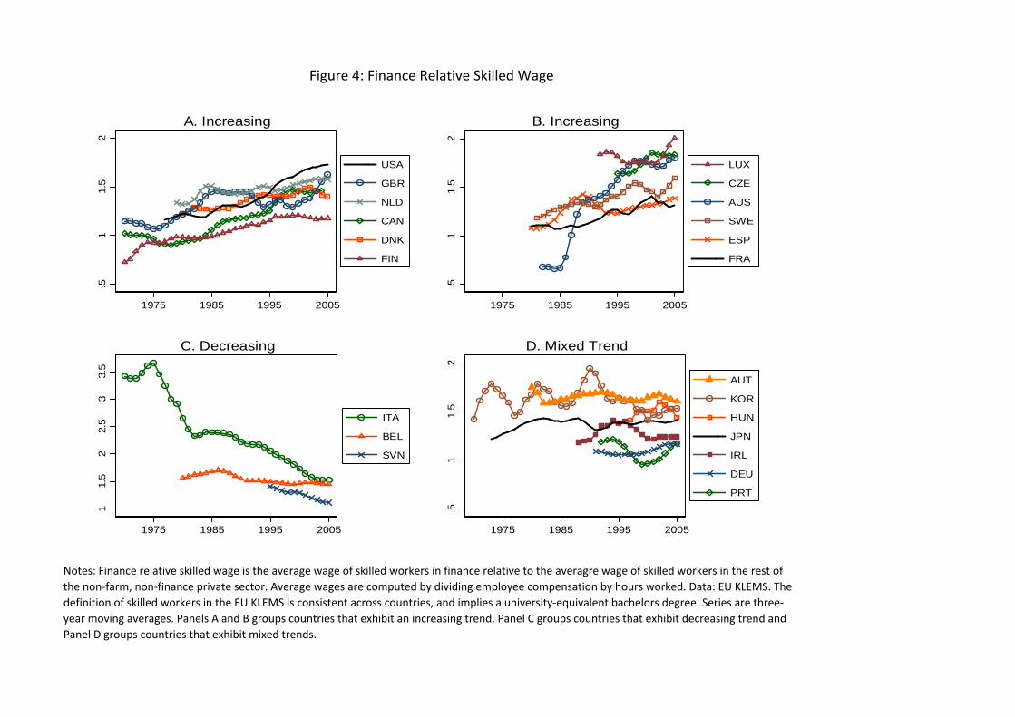
Figure 4: Finance Relative Skilled Wage

Notes: Finance relative skilled wage is the average wage of skilled workers in finance relative to the averagre wage of skilled workers in the rest of

the non-farm, non-finance private sector. Average wages are computed by dividing employee compensation by hours worked. Data: EU KLEMS. The

definition of skilled workers in the EU KLEMS is consistent across countries, and implies a university-equivalent bachelors degree. Series are three-

year moving averages. Panels A and B groups countries that exhibit an increasing trend. Panel C groups countries that exhibit decreasing trend and

Panel D groups countries that exhibit mixed trends.

.51

1.5

2

1975 1985 1995 2005

USA

GBR

NLD

CAN

DNK

FIN

A. Increasing

.51

1.5

2

1975 1985 1995 2005

LUX

CZE

AUS

SWE

ESP

FRA

B. Increasing

11.

52

2.5

33.

5

1975 1985 1995 2005

ITA

BEL

SVN

C. Decreasing

.51

1.5

2

1975 1985 1995 2005

AUT

KOR

HUN

JPN

IRL

DEU

PRT

D. Mixed Trend

Figure 5: Finance Relative Skill Intensity

Notes: Finance relative skill intensity is the share of college-educated workers in finance relative to the

share of college-educated workers in the rest of the non-farm, non-finance private sector. These

shares are computed using hours worked. Data: EU KLEMS. The definition of skilled workers in the EU

KLEMS is consistent across countries, and implies a university-equivalent bachelors degree. Series are

three-year moving averages. Panel A groups countries that exhibit an increasing trend. Panel B groups

countries that exhibit mixed trends.

0.1

.2.3

1970 1975 1980 1985 1990 1995 2000 2005

JPN

ESP

FIN

PRT

USA

BEL

AUS

FRA

CAN

NLD

DNK

A. Consistently Increasing

-.05

0.0

5.1

.15

.2

1970 1975 1980 1985 1990 1995 2000 2005

IRL

HUN

CZE

SVN

SWE

LUX

GBR

ITA

AUT

DEU

KOR

B. Other Trends

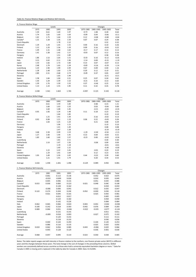
1975 1985 1995 2005 1975-1985 1985-1995 1995-2005 Total

Australia 1.34 0.61 1.69 1.97 -0.73 1.08 0.28 0.63

Austria 1.74 1.65 1.69 1.63 -0.09 0.04 -0.06 -0.11

Belgium 1.62 1.75 1.66 1.59 0.12 -0.08 -0.08 -0.04

Canada* 1.21 1.28 1.35 1.59 0.07 0.07 0.24 0.38

Czech Republic 1.78 2.10 0.32 0.32

Denmark 1.29 1.29 1.45 1.55 0.00 0.16 0.10 0.26

Finland 1.12 1.20 1.36 1.33 0.09 0.16 -0.03 0.22

France 1.49 1.31 1.48 1.62 -0.17 0.17 0.14 0.13

Germany 1.41 1.38 1.45 1.57 -0.03 0.07 0.12 0.16

Hungary 1.51 1.89 0.38 0.38

Ireland 1.86 1.53 1.64 1.51 -0.33 0.10 -0.12 -0.35

Italy 3.15 2.02 2.11 1.96 -1.14 0.09 -0.15 -1.19

Japan 1.53 1.66 1.73 1.66 0.13 0.07 -0.07 0.13

Korea 2.48 1.79 1.63 1.34 -0.69 -0.16 -0.29 -1.14

Luxemburg 1.23 1.90 1.99 2.39 0.67 0.09 0.40 1.16

Netherlands 1.28 1.48 1.60 1.79 0.20 0.12 0.19 0.51

Portugal 2.80 2.31 2.68 2.73 -0.49 0.37 0.05 -0.07

Slovenia 1.65 1.44 -0.21 -0.21

Spain 1.58 1.84 1.90 2.21 0.25 0.07 0.30 0.62

Sweden 1.50 1.29 1.39 1.52 -0.21 0.10 0.13 0.02

United Kingdom 1.39 1.76 1.30 1.55 0.37 -0.46 0.25 0.16

United States 1.13 1.24 1.55 1.90 0.11 0.32 0.35 0.78

Average 1.638 1.541 1.663 1.765 -0.097 0.125 0.102 0.126

1975 1985 1995 2005 1975-1985 1985-1995 1995-2005 Total

Australia 0.61 1.59 1.83 0.98 0.23 1.21

Austria 1.60 1.63 1.59 0.03 -0.04 0.00

Belgium 1.69 1.48 1.45 -0.21 -0.03 -0.24

Canada* 0.95 1.06 1.24 1.48 0.11 0.18 0.23 0.53

Czech Republic 1.66 1.85 0.19 0.19

Denmark 1.25 1.41 1.39 0.16 -0.02 0.13

Finland 0.92 0.98 1.21 1.18 0.06 0.22 -0.03 0.26

France 1.04 1.25 1.33 0.21 0.08 0.29

Germany 1.06 1.15 0.10 0.10

Hungary 1.41 1.49 0.08 0.08

Ireland 1.47 1.28 -0.19 -0.19

Italy 3.68 2.39 2.09 1.53 -1.29 -0.30 -0.56 -2.15

Japan 1.27 1.40 1.44 1.41 0.13 0.04 -0.03 0.15

Korea 1.83 1.60 1.60 1.57 -0.23 0.00 -0.03 -0.26

Luxemburg 1.81 2.11 0.30 0.30

Netherlands 1.53 1.47 1.56 -0.06 0.09 0.03

Portugal 1.19 1.18 -0.01 -0.01

Slovenia 1.40 1.10 -0.30 -0.30

Spain 1.22 1.22 1.41 -0.01 0.20 0.19

Sweden 1.29 1.41 1.64 0.12 0.23 0.35

United Kingdom 1.05 1.49 1.26 1.65 0.44 -0.22 0.39 0.60

United States 1.21 1.41 1.74 0.20 0.34 0.53

Average 1.616 1.358 1.441 1.496 -0.129 0.089 0.056 0.081

1975 1985 1995 2005 1975-1985 1985-1995 1995-2005 Total

Australia 0.061 0.113 0.136 0.052 0.023 0.075

Austria -0.019 -0.009 0.026 0.010 0.035 0.045

Belgium 0.045 0.096 0.131 0.051 0.035 0.086

Canada* 0.015 0.036 0.083 0.123 0.021 0.048 0.040 0.108

Czech Republic 0.128 0.162 0.034 0.034

Denmark -0.006 0.006 0.041 0.012 0.035 0.047

Finland 0.122 0.174 0.204 0.240 0.052 0.030 0.036 0.118

France 0.021 0.045 0.101 0.025 0.056 0.081

Germany 0.012 0.017 0.005 0.005

Hungary 0.124 0.182 0.058 0.058

Ireland 0.142 0.226 0.084 0.084

Italy 0.062 0.065 0.066 0.024 0.003 0.001 -0.042 -0.038

Japan 0.100 0.142 0.218 0.303 0.042 0.076 0.084 0.203

Korea 0.089 0.066 0.031 -0.046 -0.022 -0.035 -0.077 -0.134

Luxemburg 0.131 0.141 0.011 0.011

Netherlands -0.009 0.018 0.093 0.027 0.075 0.102

Portugal 0.120 0.231 0.111 0.111

Slovenia 0.118 0.155 0.036 0.036

Spain 0.040 0.144 0.293 0.104 0.149 0.253

Sweden 0.086 0.110 0.135 0.025 0.025 0.050

United Kingdom 0.019 0.062 0.056 0.085 0.043 -0.006 0.029 0.066

United States 0.093 0.128 0.129 0.036 0.001 0.036

Average 0.068 0.057 0.095 0.133 0.023 0.030 0.038 0.065

Table A1: Finance Relative Wages and Relative Skill Intensity

Levels Changes

Notes: The table reports wages and skill intensity in finance relative to the nonfarm, non-finance private sector (NFFP) in different

years and the changes between those years. The total change is the sum of changes in the preceding three columns. Skilled

workers are consistently defined across countries as those who hold a university-equivalent bachelors degree or more. * Data for

Canada in 2005 is missing and is replaced in this table by data for Canada in 2004. Data: EU KLEMS.

B. Finance Relative Skilled Wage

A. Finance Relative Wage

Levels Changes

C. Finance Relative Skill Intensity

Levels Changes

Finance relative

ICT intensity Domestic credit

Non-bank

domestic

credit/GDP

Bank domestic

credit/GDP

Household bank

credit/GDP

Corporate bank

credit/GDP

Financial

globalization

Deregulation

Index

International

capital

restrictions Privatization Entry barriers

Banking

supervision Directed credit

Interest

rate

control

Finance relative ICT intensity 1

Domestic credit/GDP 0.13 1

Non-bank domestic credit/GDP 0.03 0.87 1

Bank domestic credit/GDP 0.22 0.46 -0.04 1

Household bank credit/GDP 0.29 0.03 -0.36 0.71 1

Corporate bank credit/GDP 0.06 0.64 0.30 0.75 0.08 1

Financial globalization 0.47 0.04 -0.27 0.57 0.76 0.10 1

Deregulation Index 0.38 0.28 0.08 0.43 0.59 0.07 0.76 1

International capital restrictions 0.27 0.35 0.23 0.30 0.31 0.14 0.49 0.82 1

Privatization 0.05 0.33 0.21 0.30 0.52 -0.01 0.39 0.63 0.49 1

Entry barriers 0.54 0.15 -0.09 0.48 0.56 0.15 0.75 0.76 0.51 0.23 1

Banking supervision 0.29 0.25 0.07 0.40 0.52 0.07 0.62 0.84 0.58 0.46 0.65 1

Directed credit 0.37 0.00 -0.10 0.17 0.53 -0.20 0.61 0.78 0.56 0.53 0.65 0.57 1

Interest rate control 0.25 0.19 0.03 0.32 0.32 0.17 0.63 0.72 0.60 0.22 0.50 0.51 0.43 1

Finance relative

ICT intensity Domestic credit

Non-bank

domestic

credit/GDP

Bank domestic

credit/GDP

Household bank

credit/GDP

Corporate bank

credit/GDP

Financial

globalization

Deregulation

Index

International

capital

restrictions Privatization Entry barriers

Banking

supervision Directed credit

Interest

rate

control

Finance relative ICT intensity 1

Domestic credit/GDP 0.08 1

Non-bank domestic credit/GDP -0.12 0.58 1

Bank domestic credit/GDP 0.21 0.65 -0.25 1

Household bank credit/GDP 0.21 0.54 -0.22 0.85 1

Corporate bank credit/GDP 0.17 0.57 -0.20 0.87 0.49 1

Financial globalization 0.14 0.21 -0.02 0.26 0.15 0.29 1

Deregulation Index -0.29 0.03 0.04 0.00 -0.09 0.08 0.03 1

International capital restrictions -0.18 -0.05 -0.04 -0.03 -0.08 0.03 0.02 0.63 1

Privatization -0.03 -0.08 -0.10 0.00 0.07 -0.06 -0.01 0.28 -0.02 1

Entry barriers -0.17 0.05 0.05 0.01 -0.12 0.13 0.03 0.61 0.32 0.07 1

Banking supervision -0.15 0.00 -0.05 0.05 0.01 0.05 -0.11 0.44 0.11 0.13 0.20 1

Directed credit -0.11 -0.06 -0.08 0.01 -0.03 0.04 0.09 0.56 0.29 0.05 0.31 0.10 1

Interest rate control -0.14 0.10 0.13 -0.01 -0.12 0.10 0.08 0.45 0.18 -0.07 0.03 -0.09 0.16 1

A. Correlations across variables in levels

Table A2: Correlations for Level and Predictive Regressions

B. Correlations across variables in changes (t-3,t)

Notes: Statistics are computed for 356 observations for 15 countries. The range for t is 1976-2005. Wage, skill and ICT variables are calculated based on EU KLEMS data. Domestic credit covers all forms of credit to the non-financial sector on a gross level, except for credit to the

government, which is on a net basis; data from the World Bank World Development Indicators databse. Bank domestic credit data are from Jorda, Schularick and Taylor (2014), except for Austria and Korea where the data are from the Bank World Development Indicators databse. Non-bank

domestic credit is total domestic credit minus bank credit. The split of bank domestic credit to households versus corporations is given in Jorda, Schularick and Taylor (2014). Financial globalization is log(foreign assets + liabilities/GDP), data are from Lane and Milesi-Ferretti (2007). Statistics

on the financial reform indices are reported in Table 5. All correlation coefficients that are strictly greater than 0.11 are statistically significant at the 5% level; in Panel B most correlation coefficients are not statistically significant at conventional levels.

Finance relative

ICT intensity Domestic credit

Non-bank

domestic

credit/GDP

Bank domestic

credit/GDP

Household bank

credit/GDP

Corporate bank

credit/GDP

Financial

globalization

Bank

concentration

Finance relative ICT intensity 1

Domestic credit/GDP -0.14 1

Non-bank domestic credit/GDP -0.06 0.89 1

Bank domestic credit/GDP -0.17 0.15 -0.31 1

Household bank credit/GDP -0.10 -0.25 -0.55 0.69 1

Corporate bank credit/GDP -0.12 0.45 0.09 0.77 0.12 1

Financial globalization 0.18 -0.49 -0.69 0.49 0.78 0.04 1

Bank concentration 0.19 -0.61 -0.76 0.36 0.27 0.27 0.39 1

Table A3: Correlations for Bank Concentration Regressions

Notes: Bank concentration is the log of the share of the largest three banks; data from the World Bank. Domestic credit covers all forms of credit to the non-financial sector on a gross

level, except for credit to the government, which is on a net basis; data from the World Bank World Development Indicators databse. Bank domestic credit data are from Jorda,

Schularick and Taylor (2014), except for Austria and Korea where the data are from the Bank World Development Indicators databse. Non-bank domestic credit is total domestic credit

minus bank credit. The split of bank domestic credit to households versus corporations is given in Jorda, Schularick and Taylor (2014). Financial globalization is log(foreign assets +

liabilities/GDP), data are from Lane and Milesi-Ferretti (2007). Statistics are computed for 60 observations for 16 countries. The range for t is 2000-2005. The sample of 16 countries is

determined by ICT data availability in the EU KLEMS data; these countries are: Australia, Austria, Canada, Czech Republic, Germany, Denmark, Finland, United Kingdom, Italy, Japan,

Korea, Netherlands, Portugal, Sweden, United States, Slovenia. All correlations above 0.3 are statistically significant.

(1) (2)

Second Stage Dependent Variable: Changes from t to t+3 in Relative Wage Relative Skilled Wage

Financial deregulation, t-3 -0.0936** -0.183***

(0.0367) (0.0329)

Change in finance relative share of ICT in capital stock, t-3 to t -0.511*** -0.380***

(0.141) (0.126)

Change in domestic credit/GDP, t-3 to t 0.0770** 0.0129

(0.0374) (0.0416)

Change in financial globalization, t-3 to t 0.0269 0.0349

(0.0255) (0.0239)

Observations 293 293

R-squared 0.248 0.275

Instrument: Financial deregulation, t-3

Table A4: Finance Relative Wage and Relative Skill Intensity, Predictive Regressions, TSLS --- First Stage Regressions

Notes: All regressions include country fixed effects. Deregulation data are from Abiad, Detragiache and Tressel (2008). The dependent

variables as well as relative ICT use in finance is calculated from EU KLEMS database. Domestic credit is normalized by GDP, data from the

World Bank World Development Indicators databse. Financial globalization is log(foreign assets + liabilities/GDP), data are from Lane and

Milesi-Ferretti (2007). The sample ends in 2005. Robust standard errors in parentheses. *** p<0.01, ** p<0.05, * p<0.1.

Instrumented, Dependent Variable: Change in financial deregulation, t-3 to t

Destination AUS AUT DNK FIN HUN IRL ITA LUX PRT Total

AUS 0 0 0 0 0 0 0 1 0 1

DNK 0 0 0 0 0 0 0 1 0 1

ESP 1 0 0 1 1 0 0 1 0 4

FIN 0 0 0 0 1 0 1 1 1 4

HUN 0 0 1 1 0 1 0 1 1 5

PRT 0 1 0 0 1 0 0 0 0 2

Total 1 1 1 2 3 1 1 5 2 17

Destination AUS AUT DNK ESP FIN HUN IRL LUX SWE Total

AUS 0 0 0 0 0 0 0 1 0 1

CAN 0 0 0 0 0 0 0 1 0 1

ESP 0 1 0 0 0 1 0 0 0 2

FIN 0 0 0 1 0 0 1 0 0 2

HUN 1 0 1 0 1 0 1 1 1 6

IRL 0 0 1 0 0 0 0 1 0 2

PRT 0 0 0 0 1 1 0 0 0 2

SWE 0 0 0 0 0 0 0 1 0 1

Total 1 1 2 1 2 2 2 5 1 17

Notes: The table reports missing (those with the value of zero) bilateral observations in the OECD immigration

data for the finance sector. Although there are 17 missing observations for each type of worker employed in

finance, these missing observations overlap in only 7 cases.

Table A5: Missing Observations on Finance Immigrants

Origin

A. Skilled Immigrants

A. Unskilled Immigrants

Origin