volatility and directional information-based trading in ... · volatility and directional...
TRANSCRIPT

Volatility and Directional Information-Based Trading in
Options
Yong Jin Mahendrarajah Nimalendran Sugata Ray1
JEL Classifications: D53, G12, G28
Keywords: Option market microstructure, Probability of informed volatility
trading (VolPIN), Probability of informed direcitonal trading (DirPIN), PIN
December 10, 2013
1Yong (Jimmy) Jin, Mahendrarajah Nimalendran, and Sugata Ray, Warrington College of BusinessAdministration, University of Florida, P.O. Box 117168, University of Florida, Gainesville FL 32611-7168. Jin: [email protected]; Nimalendran: [email protected]; Ray: [email protected];.

Volatility and Directional Information-Based Trading in
Options
Abstract
We develop a sequential trade model and estimate the probability of volatility information
trading (V olPIN) and the probability of directional information trading (DirPIN) in the
options market using high frequency individual stock options data. We find that informed
trading in options has a significant impact on price discovery of the underlying asset and
market microstructure of the options market. In particular, DirPIN has a positive effect on
stock returns and a stock with a 10 % higher DirPIN relative to the average DirPIN leads
to a 1.8% per year increase in expected returns; V olPIN predicts future unpriced volatility.
Both PIN measures are significant determinants of option spreads, explaining up to 30% of
the bid-ask spread.

1 Introduction
The process by which information is revealed through trading has been studied extensively.2
Most of this research focuses on directional information, with much less attention given to
the question of how and where information concerning volatility is revealed.3 Compelling
evidence from the time-series and option-pricing literatures indicates that volatility is time-
varying and stochastic. Also, there is a large literature on the relation between future
volatility and option implied volatility. Yet we know little about the extent to which new
information about future volatility is revealed through the trading process. Presumably,
investors with private information about volatility will trade in instruments whose price is
sensitive to volatility, an obvious choice being the options market.4
In this paper, we investigate information based trading on the options market. We
propose a structural model in the spirit of Easley, Kiefer, O’Hara, and Paperman (1996)
and Easley, Hvidkjaer, and O’Hara (2002) to measure the probability of both volatility and
directional information based trading on the options market.5 The model assumes that each
period, there is some probability of an information event. Conditional on the informational
event, the information can be either about volatility or direction with a certain probability,
further we condition the volatility and directional information based on whether it is bullish
or bearish. This results in traders placing orders in accordance with the newly created
information structure, resulting in a rich sequential trade model. Using high frequency
transaction level data and trade direction (buyer initiated and seller initiated) for calls
and puts on individual stock options we estimate the model using maximum likelihood
techniques and obtain separate estimates for the the probabilities of volatility and directional
information-based trading in individual stock options.
Informed directional traders will buy calls and/or sell puts if they are bullish on the price
and sell calls and buy puts when bearish. In contrast, informed volatility traders will buy
calls and buy puts (a straddle) if they are bullish on volatility and sell straddles if they are
2Theoretical underpinnings of this literature include Glosten and Milgrom (1985), Kyle (1985), and Easley,Kiefer, O’Hara, and Paperman (1996) Empirical work in this area is described in Hasbrouck (1995).
3In our study, directional information refers to information about whether a stock price is going up ordown. Volatility information refers to information regarding the future volatility of a stock either increasingor decreasing.
4Recently there have been ETFs on VIX as well as futures on VIX that can be traded. However, we arenot aware of securities on individual stock volatility.
5 Ni, Pan, and Poteshman (2008) [NPP] also investigate informed trading on volatility in the optionsmarket using daily net non-market maker trading volume on calls and puts to construct a measure fortrading on volatility information. We discuss the differences in our studies and findings in the followingsection.
1

bearish. In addition there will be noise or uninformed traders who will be buying and selling
calls and puts. These trading choices provide identification to estimate separate probabilities
of informed trading for directional and volatility trading, which we term DirPIN , and
V olPIN , respectively.
We validate our estimated V olPIN and DirPIN measures by confirming that they
are correlated with intuitively linked observable variables. For example, periods with high
V olPIN are followed by periods with high absolute unpriced volatility (|realized volatility
minus option price implied volatility|). Similarly, we find DirPIN is positively correlated
with the Easley, Kiefer, O’Hara, and Paperman (1996) stock PIN measure, with a correla-
tion of 0.22, while V olPIN has a weaker correlation of .09. We also find that V olPIN and
DirPIN are higher prior to earnings announcements.
We use the estimatedDirPIN and V olPIN together with stock PIN to estimate relative
contributions to asset returns, and bid-ask spreads. We find that the V olPIN and DirPIN
are both significantly related to option market bid-ask spreads. A one standard deviation
(.066) increase in the V olPIN increases relative bid ask spreads by 0.34% and a one standard
deviation (.066) increase in DirPIN increases relative bid ask spreads by 0.73%. Based on
an average spread of 5.8% in the options market, the effect of one standard deviation increase
in volatility and directional information risks in options lead to a 18% increase in spreads.
We also find that the DirPIN is positively linked to future abnormal returns for the
stock. Following the model outlined in Easley, Hvidkjaer, and O’Hara (2002), investors
holding stocks with higher amount of informed trading expect a higher return for the in-
formational risks they face. We find that a stock with a 10% higher DirPIN is associated
with a 1.8% increase in expected returns. The V olPIN does not significantly affect stock
returns. Easley, Hvidkjaer, and O’Hara (2002) find a similar link with the stock PIN as
our findings regarding the DirPIN , documenting a 2.5% higher return for stock with a 10%
larger stock PIN . Interestingly, in our study, the stock PIN is not a significant determinant
of expected returns returns based on Fama-MacBeth regression model. This may be due to
our using only the largest stocks, where more informed trading may be carried out in the
option markets, or a difference in time periods used for the sample.
Our findings are consistent with informed trading in option markets affecting both the
market microstructure of the options market and also future asset returns. Our main contri-
butions are: (1) The construction and estimation of a information risk measure for options
markets, (2) a decomposition of option market bid/ask spreads to include the effects of
asymmetric information about both direction and volatility, as well as the hedging and re-
balancing costs associated delta hedging, (3) linking the directional DirPIN measure from
2

option markets to asset returns, and (4) documenting information-based trading prior to
earnings announcements.
2 Literature review
There is a rich literature covering directional informed trading and its link to market mi-
crostructure 6. The literature examining directional informed trading in both stock and
option markets is narrower, with theoretical roots in Easley, O’hara, and Srinivas (1998)
which proposes a theoretical model, with directionally informed traders choosing between
stock and option markets based on the transaction costs in the markets and the “bang-for-
buck” in the form of leverage, afforded by the options market. The authors conclude there
may be a separating equilibrium, where informed traders trade only in the stock market,
or a pooling equilibrium, where informed traders trade in both, depending on the relative
transaction costs differences in these markets.
Subsequent empirical work focused on directional informed trading in these two venues
has largely supported the theoretical predictions in the model (e.g. Cao, Chen, and Griffin
(2005) which studies option trading prior to takeovers) or extended the framework to include
other interactions between the two markets (e.g. Huh, Lin, and Mello (2012) which allows
the market makers in the option markets to hedge in the stock market).7
The literature examining informed volatility trading is more recent. Johnson and So
(2013), which estimates a multi-market information asymmetry measure, similar to the PIN ,
for option markets using aggregate unsigned volume. While simple to compute as it does
not rely on estimation of a structural model, it includes both information on volatility and
direction in one measure.
Ni, Pan, and Poteshman (2008) (NPP) use trades by non-market makers in the option
markets to estimate demand for volatility and show that this demand is “informative about
the future realized volatility of underlying stocks.” In contrast to our study, which uses
intraday quote and transaction data to sign trades, NPP use non-market maker volume
(NMMV ), obtained from the Chicago Board of Options Exchange (CBOE) at the daily level
for their analysis. Additionally, rather than estimating PIN measures, the study separates
6Bagehot (1971), Glosten and Milgrom (1985), Kyle (1985), Easley and O’hara (1987)7More generally, numerous authors have examined informed trading in option markets, for example,
Chakravarty, Gulen, and Mayhew (2004), and Kaul, Nimalendran, and Zhang (2004) but these authorsfocus on directional information about the underlying stock price, not information about the volatility.Simaan and Wu (2007) examine price discovery across option exchanges, but they make no attempt todifferentiate between option price changes resulting from underlying stock price changes and those resultingfrom volatility changes.
3

option volume into trades that could have been used for constructing straddles and those that
were not. Their findings relating informed volatility trading, estimated using NMMV , to
future changes in volatility closely mirror our own findings regarding the V olPIN and future
volatility. In our study, we separately estimate measures for directional and volatility based
information trading in the options market. While NPP largely disregard “non-straddle”
trading, exclusively focusing on straddle trades, we holistically characterize trades as noise,
directional, or volatility information driven, and separately estimate measures for volatility
and directions information-based trades.
The advantages of our analysis over NPP include: (1) Using intraday data that allow us
to sign trades individually, rather than relying on aggregate daily volume.(2) Examining the
contribution of both volatility and directional information-based risk measures to explain
simultaneously using the PIN framework allows us to assess asset pricing implications of the
two measures separately and to decompose their effect on the option market bid ask spread.
3 Model
In this section we outline our information-based trading model that captures both directional
information and volatility information. Our sequential trade model is a generalization of
Easley, Kiefer, O’Hara, and Paperman (1996) and Easley, Hvidkjaer, and O’Hara (2002)’s
probability of information-based trade (PIN) model.
Our model extends their model to the options market where agents can trade on direc-
tional information as well as volatility information on the underlying stock. Traders having
information about the future increase in stock price can use a long call/short put strategy
and long put/short call strategy for information on future decrease in stock price. If the
information is about volatility, then they can employ a long straddle (long call and long put)
when the information is about an increase in volatility and short straddle for a decrease in
future volatility.
In our model, new information arrives every 30 minutes with probability α and, con-
ditional on a information event, it is either volatility information with probability θ or
directional information with probability 1 − θ. Volatility information can be high (prob δ)
or low (prob 1− δ). Directional information is either good news (prob γ) or bad news (prob
1− γ).
Orders from informed and uninformed traders to buy/sell, call/put options follow in-
dependent Poisson processes. Uninformed buyers (seller) arrive according to independent
4

Poisson processes at rate ε ∈ {εBC , εSC , εBP , εSP}, where the subscripts C and P denote calls
and puts, and superscripts B and S denote buys and sells by the traders. Orders from
traders possessing volatility information arrive at rates µ ∈ {µBC , µBP } for high volatility,
and {µSC , µSP} for low volatility. Finally, orders from informed directional traders arrive at
rate ν ∈ {νBC , νSP} for high direction, and {νSC , νBP } for low direction. Figure 1 shows the
information and the decision tree for the traders’ strategies.
When there is no information in the market (1 − α), the orders are purely uninformed,
with arrival rates εBC , εSC , ε
BP , ε
SP for long call, short call, long put, short put respectively. When
information event occurs in the market (α), and the information is about volatility (θ), and
if the volatility is high (δ), the joint probability of high volatility information event is αθδ.
Under this situation, the market orders arrive rates µBC + εBC , εSC , µ
BP + εBP , ε
SP for long call,
short call, long put, short put respectively. Similarly, we have the probabilities and arrival
rates for each of the five end nodes in the tree. Based on these assumptions we can derive
the likelihood function conditional on number of buys(B), sells (S) for call (C) and put (P )
options.
3.1 Likelihood Function and Estimation
The likelihood function given the model is based on the following assumptions. 1) There is
only one information event in the defined unit period (in our estimation we use 30 minutes
in a day); (2) There is no possibility of volatility information and direction information
occurring simultaneously. Then the marginal likelihood function one period is given by
equation 1, where we have suppressed the subscript t.
l(Θ|Orders) =(1− α)e−εBC
(εBC)CB
CB!e−ε
SC
(εSC)CS
CS!e−ε
BP
(εBP )PB
PB!e−ε
SP
(εSP )PS
PS!
+ αθδe−(µSC+εBC ) (µ
SC + εBC)CB
CB!e−ε
SC
(εSC)CS
CS!e−(µ
BP+εBP ) (µ
BP + εBP )PB
PB!e−ε
SP
(εSP )PS
PS!
+ αθ(1− δ)e−εBC (εBC)CB
CB!e−(µ
SC+εSC) (µ
SC + εSC)CS
CS!e−ε
BP
(εBP )PB
PB!e−(µ
SP+εSP ) (µ
SP + εSP )PS
PS!
+ α(1− θ)γe−(νSC+εBC ) (νSC + εBC)CB
CB!e−ε
SC
(εSC)CS
CS!e−ε
BP
(εBP )PB
PB!e−(ν
SP+εSP ) (ν
SP + εSP )PS
PS!
+ α(1− θ)(1− γ)e−εBC
(εBC)CB
CB!e−(ν
SC+εSC) (ν
SC + εSC)CS
CS!e−(ν
BP+εBP ) (ν
BP + εBP )PB
PB!e−ε
SP
(εSP )PS
PS!(1)
5

3.1.1 Simplified Model
The model give by equation 1 has 16 parameters, and estimating all the parameters using
MLE is challenging. To make the model tractable we impose several restrictions. First, we
set all the uninformed arrival rates to be the same ε = εBC = εSC = εBP = εSP . This is not a very
restrictive assumption as these are non-strategic traders. Second, we set the informed arrival
rates for high and low volatility traders to be the same, µ = µBC = µSC = µBP = µSP . This is
more restrictive as one might expect arrival rates for high volatility to be different from low
volatility. Finally, we assume that the arrival rates for the high and low directional trader to
be the same, ν = νBC = νSC = νBP = νSP . We do not expect directional traders to prefer high
or low directional trades and hence this assumption is not restrictive. These assumptions
reduce the number of parameters to be estimated to 7 from 16 and the likelihood function
is given by equation 2:
l(Θ|Orders) =1
CB!CS!PB!PS!{(1− α)e−εεCBe−εεCSe−εεPBe−εεPS
+ αθδe−(µ+ε)(µ+ ε)CBe−εεCSe−(µ+ε)(µ+ ε)PBe−ε(ε)PS
+ αθ(1− δ)e−εε)CBe−(µ+ε)(µ+ ε)CSe−εεPBe−(µ+ε)(µ+ ε)PS
+ α(1− θ)γe−(ν+ε)(ν + εBC)CBe−εεCSe−εεPBe−(ν+ε)(ν + ε)PS
+ α(1− θ)(1− γ)e−εεCBe−(ν+ε)(ν + ε)CSe−(ν+ε)(ν + ε)PBe−εεPS}
=1
CB!CS!PB!PS!e−4ε{(1− α)εCB+CS+PB+PS + αθδe−2µεCS+PS(µ+ ε)CB+PB
+ αθ(1− δ)e−2µε)CB+PB(µ+ ε)CS+PS + α(1− θ)γe−2νεCS+PB(ν + ε)CB+PS
+ α(1− θ)(1− γ)e−2µεCB+PS(ν + ε)CS+PB}(2)
The log likelihood function is given by,
L(Θ|Orders) = Log(T∏t=1
lt). (3)
We use a maximum likelihood method (MLE) to estimate the parameters of the model,
Θ = {α, δ, θ, γ, ε, µ, ν}, using signed orders Orders ∈ {CB,CS, PB, PS} for individual
stock options. From these estimates we construct estimates for the probability of volatility
informed trading (V olPIN) and directional informed trading (DirPIN).
6

3.2 Information-Based Measures; V olPIN and DirPIN
3.2.1 Simplified Model
The probability of volatility information is αθ, and conditional on this the expected informed
arrival rate is 2(δµ + (1− δ)µ) = 2µ. Hence the expected rate of volatility informed arrival
is 2αθµ. Similarly, the expected directional informed arrival rate is 2α(1 − θ)ν. The total
expected uninformed arrival rate is 4ε. Based on this the information measures V olPIN
and DirPIN are give by the following equations.
V olPIN =αθµ
αθµ+ α(1− θ)ν + 2ε(4)
DirPIN =α(1− θ)ν
αθµ+ α(1− θ)ν + 2ε(5)
We use a 30 minute interval during a day as the time period, and use two weeks of
observations for t. Since each day has 6.5 hours of trading, we get 13 observations per day
and over two weeks, we obtain 130 (T ) observations for the estimation. In the following
section, we use Monte Carlo simulation techniques to ascertain the finite sample properties
of the estimators and ensure parameter recovery using 130 periods is possible and accurate.8
4 Monte Carlo Simulation
We follow the approach used by Nimalendran (1994) to carry our Monte Carlo simulation
for estimating and analyzing the finite sampe properties of the sample parameter estimators.
In this study we use R-Project software to generate simulated samples and obtain the
finite sample behavior using the following procedure.
1. We first set the values for the parameters (α, θ, δ, γ, ε, µ, ν).
8Note that the term CB!CS!PB!PS! can be factored out for the marginal likelihood function. Thisterm does not involve any of the parameters. Hence, in the MLE procedure we eliminate the term from loglikelihood function.
7

2. Generate four independent and identical uniformly (0, 1) random variables to decide the
“No information, High Vol information, Low Vol information, High Dir information,
Low Dir information” state. For example if α = .5, and the generated Uniform variable
is less than .5 then we will be in the no information state. Similarly for the other states
of the tree.
3. Once the terminal node of the tree is determined, we use the given parameters to
simulate the number (volume) of orders of long call, short call, long put, short put for
a certain fixed observations of periods (T = 100 or T = 300), thus a sample including
T observation of Orders ∈ {CB,CS, PB, PS} is generated.
4. Use non-linear optimization tools to estimate the parameters by maximizing the log-
likelihood function, and then record the estimated parameters as (α̂1, δ̂1, θ̂1, γ̂1, ε̂1, µ̂1, ν̂1).
5. Repeat steps 2-4 for 200 replications and record the estimated parameters as,
(α̂i, δ̂i, θ̂i, γ̂i, ε̂i, µ̂i, ν̂i), where i = 1 : 200.
6. After obtaining the set of all the estimated parameters, we calculate the number
of replications for which the optimization converged to feasible estimates (NC), the
mean estimates MEAN = 1NC
∑NCi=1 η̂i and the standard errors of the means SEM =
1√NC
[ 1(NC−1)
∑NCi=1(η̂i −MEAN)2]1/2, where η ∈ {α, δ, θ, γ, ε, µ, ν}.
The results of our simulation is presented in Table 1. We present six set of parameter
choices and two sets of number of observations (100, and 300). The parameters (α, θ, δ, γ)
are chosen to be between 0.3 and 0.7. While the arrival rates for traders is chosen to be (50,
100, or 150) in different combinations. We find that the number of convergences were close
to 100%. The estimators also have very good finite sample properties. The bias for all the
estimators are very small, and the standard error of the estimates are also very small. For
example, the percentage of estimation error of α varies from 0 to 1.2% and the absolute value
of t-test which is the bias/SEM varies from 0 to 0.125, which cannot reject the null that
the estimates are different from the parameters. The efficiency of the estimators improves
when more observations enter the simulated sample, which is the same as our expectation.
Different combinations of parameters also provide information of sensitivity but overall, our
simulation shows that the procedure is efficient and accurate to get the estimates for the
parameters for our Option PIN model using 130 observations.
8

5 Data and summary statistics
5.1 Data
In this paper, all the option transaction level data are obtained from OPRA Option Database.
This data was provided by the OptionData warehouse, Baruch College, CUNY.9 The stock
transaction level data are extracted from the Trade and Quote (TAQ) Database. Other
option data such as option Greeks, implied volatility, and realized volatility are obtained
from Optionmetrics Database. Finally, the stock data such as end of day price, ask price, bid
price, shares outstanding, traded volume are obtained from Center for Research in Security
Prices (CRSP).
5.2 V olPIN and DirPIN Estimation Details
We construct our sample using the following procedure: 1) Compile a list of all the stocks in
TAQ and merge this list with OPRA database; 2) Sort the merged list by the option volume
in 2010 obtained from OptionMetrics, and keep the top 500 stocks. We do this to ensure
sufficient option volume to estimate our PIN measures.
For our study, we consider options within 10% of the strike price, or the nearest in-
and out- of-the-money strikes, whichever results in broader coverage. In terms of option
maturity, we keep all options expiring within 7 to 183 days. OPRA data has second level
quote data for the options markets, as well as transaction data. We use the Lee and Ready
(1991) algorithm to sign trades in both stock and option markets. Finally, we use signed
trades aggregated at 30 minute intervals (CB,CS, PB, PS) to estimate our model.
The time period of our sample (2011 calendar year) is split into 2 week estimation periods.
For each 2 week estimation period, we use 30 minute intervals to measure order flow to
compute V olPIN and DirPIN measures. For each day we have 13 30 minute observations
and over two weeks, we have 130 such observations. These 130 observations are used for our
estimates.
To estimate the PIN measure for stocks, we merge NBBO and Trades data from TAQ
and use Lee and Ready (1991) to define the stock trade direction. Similar to the process
for options, for every 30 minute interval, we calculate the volume of Trades-up (buys) and
9Option Price Reporting Authority (OPRA) was established as a securities information processor for mar-ket information, for collecting, consolidating and disseminating the option market data from its participantsincluding AMEX, ARCA, BATS, BX, BSE, C2, CBOE, ISE, MIAX, NASDAQ, and PHLX. OPRA OptionDatabase contains all the transaction level data (Trades and Quotes) for stock options which is traded inthe participants’ exchange.
9

Trades-down (sells) for each stock. We use two weeks or 10 trading days to obtain 130
observations to estimate PIN using the technique outlined in Easley, Kiefer, O’Hara, and
Paperman (1996). The stock PIN model is given in Figure 2.
5.3 Summary statistics
Table 5 presents summary statistics for option related variables in our sample. The sample
consists of 500 stocks over the 26 2-week periods in 2011. Lack of option volume, or other
variables leads to the overall sample size being around 8000 observations (rather than 500
* 26 = 13000). The average bid ask spread for options in our sample is 10.5 cents, which
translates to a relative bid ask spread of 5.8%. The average log daily volume for options
is 8.2 (or 3640 options traded). The log volume over each two week period is 10.5 (36315),
reflecting approximately 10 trading days per two week window. The Greeks for the options
are also presented. The average ∆ is 0.53, reflecting the fact that only options at or around
the money are used in the analysis.
The average option price implied volatility is 39.0% (annualized). This is slightly higher
than realized volatility (37.7%), in line with the option volatility premium documented
in previous literature. The average unpriced volatility (realized volatility minus implied
volatility) is the difference (-1.3%) and the average absolute unpriced volatility is 10.3%.
Note that informed volatility trading would be reflected in higher absolute unpriced volatility,
rather than simply unpriced volatility, as informed volatility traders may go long or short
volatility.
The variables used to construct V olPIN and DirPIN are given in Section 3. As a recap,
α is the probability that there is information in each 30 minute interval. θ is the probability
that the information is regarding direction, rather than volatility, conditional on there being
information. γ is the probability that directional information is good news rather than bad
news. δ is the probability information is regarding an increase in volatility rather than a
decrease.
V olPIN and DirPIN are estimated over 2 week horizons, by examining order flow in
each 30 minute interval in the 2 week horizon separately. We can see that the probability
of informed trading in each 30 minute horizon is 0.46, with roughly an even probability
that the information is regarding direction and volatility. Information regarding volatility is
more likely to be regarding an increase in volatility (δ = 0.613) but information regarding
direction is equally likely to reflect either good or bad news (γ = 48.5%). The overall
V olPIN and DirPIN are estimated at 0.225 and 0.202 respectively, suggesting roughly an
equal probability of informed volatility and directional trading.
10

Table 6 presents corresponding summary statistics for the underlying stocks in our sam-
ple. The average bid ask spread is 1.64 cents, corresponding to a relative bid ask spread of
4.5bps. The log volume is 15.547 (5.6 million shares) and the log market cap is 16.3 ($12BN).
The stock PIN is computed as per the technique outline in Easley, Kiefer, O’Hara, and Pa-
perman (1996). The probability of informed trading in each 30 minute windows is 0.339, and
informed traders are equally likely to trade on good news and bad news. The overall stock
PIN is estimated as 0.169, which is similar to the numbers reported by Easley, Hvidkjaer,
and O’Hara (2002).
Figure 3 presents distributions of V olPIN and DirPIN parameters in our sample. Fig-
ure 4 presents distributions of stock PIN parameters in our sample.
Table 7 presents the correlations across the various variable in the study. In line with
intuition, PIN measures (V olPIN and DirPIN and Stock PIN) are negatively correlation
with stock and option volume, as well as market cap. They are positively correlated with
bid ask spreads. Also in line with expectations, DirPIN is more positively correlated with
Stock PIN than V olPIN .
Table 8 presents selected summary statistics sorted by market capitalization quintiles.
Consistent with expectations, the probability of all types of informed trading decreases
with market capitalization, reflecting the greater transparency of larger companies. The
differences in the PINs of companies in the largest fifth are significantly different from the
PINs of companies in the smallest quartile.
6 Results and Analysis
6.1 Unpriced volatility and the V olPIN
In this section we study the relation between our option PIN measures and unpriced volatility,
UV = (|RV − IV |) using the following empirical model.
UV = β0 + β1(V olPIN) + β2(DirPIN) + γX + ε (6)
γX refers to control variables and additional interaction terms. Table 9 presents re-
gressions estimating the above equation and analysing the explanatory power of our PIN
measures on the absolute unpriced volatility (realized volatility over the next 2 weeks minus
the implied volatility in the option prices at the end of the current 2 week period). We find
V olPIN has a uniform positive relationship with unpriced volatility, with a one standard
deviation increase (0.066) in V olPIN associated with a 0.8% increase in absolute unpriced
11

volatility (based on model 3 estimate of 0.120 reported in 9). This change translates to a
7.8% increase based on the average unpriced volatility of 10.2%.
The positive relationship is strongest when the realized volatility is higher than the im-
plied volatility. The coefficient estimate increases to 0.227 after including a dummy variable
for the instances when the realized volatility is lower than the implied volatility. This leads
to nearly doubles (1.5% increase and a 15% change from the average) the impact of V olPIN
on future unpriced volatility. Our findings suggest that informed volatility trading, as esti-
mated using our V olPIN measure, is indeed linked to significantly large differences between
implied and realized volatility. Furthermore, the informed trading captured by our measure
is more likely to be trading on increasing volatility, rather than decreasing volatility.
In addition to V olPIN we find thatDirPIN too is positively related to absolute unpriced
volatility. Though, the sensitivity of 0.0541 is about half of the V olPIN effect. However,
when we interact DirPIN with the I(IV−RV ), the estimate increases to 0.0871. This is
consistent with an increase in volatility being positively related to a decrease in stock price.
Our results suggest that there is more directional informed traders in the options market
when the future volatility is higher than the implied volatility.
6.2 Asset Pricing and the DirPIN
In this section we study the relation between our option PIN measures and excess asset
returns (ER). The model is based on the study by Easley, Hvidkjaer, and O’Hara (2002).
ER = β0 + β1(Portfolioβ) + β2(StockPIN) + β3(V olPIN)+
β4(DirPIN) + β5(Log(MktCap)) + β6(StockRelSpread)+
β7(ImpliedV ol) + β8(TurnOver) + ε
(7)
Table 10 and 11 presents results of a Fama-Macbeth and fixed-effects regression model
estimates analysing the effect of our PIN measures on stock returns for the following 2
weeks. Following the model outlined in Easley, Hvidkjaer, and O’Hara (2002), we regress
daily stock returns on estimated market β, market cap, and our PIN measures. We do not
include BM variable as our data spans only one year and Easley, Hvidkjaer, and O’Hara
(2002) do not find a significant effect of this variable on returns. We find that in all the
different specifications the DirPIN to have a positive, significant relationship with future
daily stock returns. More over the coefficient estimate of 0.00362 (Model 7, Table 10) leads
to an increase in expected returns of 1.8% (based on 252 trading days) per year, for a stock
12

that has a 10% higher DirPIN relative to a stock that has average DirPIN of 0.202. Easley,
Hvidkjaer, and O’Hara (2002) using stock PIN find a 2.5% higher expected returns using a
longer time horizon and a larger cross-section of stocks.
Interestingly, the stock PIN in our analysis using Fama-MacBeth model is not a signif-
icant explanatory variable of future returns. These findings are reassuring as the intuition
outlined in Easley, Hvidkjaer, and O’Hara (2002) holds in our sample: investors in stocks
with informed trading have to be compensated for the information risk they face when trad-
ing these stocks. The fact that the Stock PIN is not significant in our analysis suggests
that for such large stocks, more of the directionally informed trading may be done in the
options markets where the transactions costs are relatively low compared to options on small
cap stocks. It also reassuring that the V olPIN is insignificant in this regression analysis
as informational risk regarding the second moment of a stock’s returns should not result in
positive returns for the stock.
The fixed effects regression estimates are shown in Table 11. In these model both Stock
PIN and DirPIN have very significant and positive coefficients. Since the fixed effect esti-
mator is based on removing the time-invariant characteristics of the assets, it is appropriate
to consider the effects as more short term in nature and less due to long term cross sectional
differences in asset returns.
Our results based on overall correlations, results regarding unpriced volatility, and asset
pricing tests are consistent with DirPIN and V olPIN being good measures of directional
and volatility based information trading in the options market.
6.3 Determinants of Option Bid-Ask Spreads
6.3.1 Adverse Selection Cost
Adverse selection costs play an important role in determining stock spreads. On the options
market, the extant evidence is mixed. If informed agents can trade strategically on the
stock and the options markets to maximize their returns from private information, and if
option market makers cannot instantaneously hedge the option exposure to adverse selection,
then the option market makers will face the same information disadvantage as stock market
makers do, and the option spread must compensate for this cost.10
Black (1975) argues that informed agents might prefer the options market for its high
leverage. On the other hand, Easley, O’hara, and Srinivas (1998) find that informed agents
10The bid-ask spreads on stocks compensate market makers for order processing, inventory (Ho and Stoll(1981)), and adverse selection costs (Bagehot (1971), Glosten and Milgrom (1985), Kyle (1985), Easley andO’hara (1987)).
13

may trade in both the option and the stock markets simultaneously. This has implications
for where price discovery occurs. The empirical evidence on this issue is mixed. For example,
Vijh (1990) and Cho and Engle (1999) find that option market makers do not face significant
adverse selection costs, while Easley, O’hara, and Srinivas (1998) and Cao, Chen, and Griffin
(2005) find evidence consistent with informed trading on the options market.
To proxy for adverse selection costs we will use DirPIN , V olPIN and Stock PIN. These
are measures of information based trading in the options market and the stock market.
6.3.2 Hedging Costs
Black and Scholes (1973) show that in a “perfect” market the payoff to an option can be
replicated by continuously unbalancing a portfolio of stocks and bonds. If the conditions
necessary for a perfect market hold, then option spreads should only compensate option mar-
ket makers for order processing costs, and perhaps for informed volatility trading. However,
when there are market frictions such as transaction costs, it is no longer possible to replicate
the option payoff using a dynamic strategy involving continuous unbalancing. Therefore,
option market makers must be compensated for the costs associated with unbalancing at
discrete time intervals, as well as costs due to market frictions such as bid-ask spread on the
underlying stock, price discreteness, information asymmetry, and model misidentification.
The costs consist of the cost of setting up and liquidating the initial delta neutral position,
and the cost to continuously rebalance the portfolio to maintain a delta neutral position.
Several papers, including Leland (1985), Merton and Samuelson (1990), and Boyle and Vorst
(1992), have theoretically examined the impact of stock bid-ask spreads on the hedging costs
imposed on option dealers due to discrete rebalancing. They show that the option spread
(the difference between the prices of long and short calls) due to the discrete rebalancing
is positively related to the proportional spread on the underlying asset, inversely related to
the revision interval, and positively related to the sensitivity of the option to changes in
volatility (vega).
Initial Hedging Cost
An option market maker would set up a delta neutral position by purchasing ∆ shares of
the stock at the ask price and close the position by selling at the bid price. This would lead
to a cost,
IC = kS∆ (8)
14

where, IC represents the initial hedging cost, k is the proportional stock spread, S is the
stock price, and ∆ is the option delta.
Rebalancing Cost
The initial hedging cost does not include the cost of rebalancing the portfolio to maintain
a delta-neutral position. Following Leland (1985) and Boyle and Vorst (1992), we define the
rebalancing cost as follows:
RC =2νk√2π(δt)
(9)
where ν is the option Vega, k is the proportional stock spread and δt is the rebalancing
interval.
The rebalancing cost is proportional to the option’s Vega and the spread on the underlying
stock, and is inversely related to the rebalancing interval. Since Vega is highest when the
stock price is equal to the present value of the exercise price, ceterisparibus, we would
expect at-the-money options to have the highest rebalancing costs. The expression for the
rebalancing costs also has an intuitive explanation the bid-ask spread on the stock gives rise
to an extra volatility when the option is replicated. For example, if you replicate a long call
option, then when the stock price increases, rebalancing would require you to purchase more
stock. But this has to be done at the ask price. Similarly, when the stock price falls, the
stock has to be sold at the bid price to maintain a delta neutral position. This effectively
increases the volatility of the asset, and this increase in volatility would be proportional to
the bid-ask spread (Roll (1984)).
In constructing the above measure of rebalancing cost we do not observe the rebalancing
frequency. Therefore, we assume that this frequency is the same across all option contracts
and drop the term√
2π(δt) in our construction of the rebalancing cost. Hence, we obtain
the following expression for rebalancing costs:
RC = νk (10)
Order Processing Costs
Since order-processing costs are likely to be fixed for any particular transaction, the order
processing costs should decrease as the expected trading volume increases. Copeland and
Galai (1983) suggest a negative relation between bid-ask spreads and trading volume in the
15

long run, and . Easley and OHara (1992) develop a model that implies spreads decrease
with an increase in expected trading volume. We use trading volume of the option contract
(number of contracts traded), denoted as OptV ol, to proxy for order processing costs. Since
we control for adverse selection, we expect the trading volume to be negatively related to
spreads.
6.3.3 A Model of Option Bid-Ask Spread
We propose the following empirical model for the determinants of option spreads.11
OptSprd = β0 + +β1(V olPIN) + β2(DirPIN) + β3(IC) + β4(RC) + β5(OptV ol) + ε (11)
Table 12 provides OLS and fixed effect regression model estimates for the above model.
We find that in all the specification, the option PIN measures and the stock PIN measure
has significant positive impact on option spreads. In OLS models, they explain nearly 31 % of
the option spreads. The economic significant of the information measures are also significant.
A one standard deviation higher probabilities of the option information measures of V olPIN
and DirPIN increase option spread by 18% from its mean value of 5.8%. Interestingly, the
stock PIN too has a significant economic impact and increases option spread by 15 %. The
findings are consistent with information traders splitting their trades between the option and
the stock markets.
6.3.4 Information Based Trading Around Earnings Announcements
In a spirit similar to NPP, we examine the effect of earnings announcement on our PIN
measures. We denote each set of PIN estimates over the 2 weeks covering an earnings
announcement as “earnings periods. The 2 weeks immediately preceding and following the
“earnings periods are denoted as “pre-earnings and “post-earnings. The remainder of the
weeks is baseline weeks.
We analyse the effects of earnings announcement by regressing V olPIN , DirPIN and
the relative bid ask spread for options on dummy variables for each of these periods. The
results are presented in Table 13. These findings are also presented graphically in Figure 5.
11We do not include the inventory costs as a determinant for two reasons. First, the literature on stockspreads suggests that its magnitude is trivial (Stoll (1989) and Madhavan and Smidt (1991)). Second, optionmarket makers rarely take directional risks. Even if they carry inventory, it is likely to be hedged.
16

We find that, in general, informed trading in option markets occurs away from earnings
periods. Both V olPIN and DirPIN measures are significantly lower during the 2 weeks
encompassing earnings announcements. The V olPIN is lower by 3% and the DirPIN is
lower by 8%. Correspondingly, the relative bid ask spreads in option markets are also the
lowest during this period (5% lower). In contrast, informed trading in the stock market is
higher during earnings periods. These results suggest that, in contrast to stock markets,
informed traders on option markets do not trade as much around earnings.
We do note that given our 2 week estimation horizon, this analysis is quite coarse, as
earnings announcements may occur towards the beginning or end of the 2 week horizon.
However, as our analysis of the preceding and subsequent 2 weeks is generally consistent with
findings for earnings weeks, this concern is not major. Additionally, this lack of precision is
likely to add noise to our analysis, and to the extent we find significant results even with
this added noise, the true results are only likely to be statistically stronger.
7 Conclusion
We estimate separate measures for the probability of informed trading in directional and
volatility information in option markets. Our option PIN measures predict future unpriced
volatility and asset prices, in line with expectations. Additionally, our option PIN measures
suggest both directionally informed and volatility informed traders contribute to the high
bid ask spreads in option markets, even after controlling for the underlying Stock PIN .
Asset pricing tests suggest the DirPIN for option markets is actually a better measure
for directional informed trading in the underlying stocks in our sample, rather than the
PIN from the stock markets. In our sample DirPIN is significantly and positively linked
to future returns, while the stock PIN only has relation in fixed effect tests. This may be
due to the shorter horizons, or the nature of large stocks used in our sample. It may also
reflect a growing trend of using option markets to trade on information. Option market
volumes have increased over the last decade, even as stock volumes have stayed largely flat.
As this volume continues to increase, and more information about both the future direction
and volatility of stocks is revealed on the option markets, analyzing the effect of informed
trading on option markets will be paramount. We hope the V olPIN and DirPIN measures,
as proposed in this study, will help with this analysis.
17

References
Bagehot, Walter, 1971, The only game in town, Financial Analysts Journal 27, 12–14.
Black, Fischer, 1975, Fact and fantasy in the use of options, Financial Analysts Journal pp.
36–72.
Black, Fischer, and Myron Scholes, 1973, The pricing of options and corporate liabilities,
The journal of political economy pp. 637–654.
Boyle, Phelim P, and Ton Vorst, 1992, Option replication in discrete time with transaction
costs, The Journal of Finance 47, 271–293.
Cao, Charles, Zhiwu Chen, and John M. Griffin, 2005, Informational Content of Option
Volume Prior to Takeovers, The Journal of Business 78, 1073–1109.
Chakravarty, Sugato, Huseyin Gulen, and Stewart Mayhew, 2004, Informed trading in stock
and option markets, The Journal of Finance 59, 1235–1258.
Cho, Young-Hye, and Robert F Engle, 1999, Modeling the impacts of market activity on bid-
ask spreads in the option market, Working paper, National Bureau of Economic Research.
Copeland, Thomas E, and Dan Galai, 1983, Information effects on the bid-ask spread, the
Journal of Finance 38, 1457–1469.
Easley, David, Soeren Hvidkjaer, and Maureen O’Hara, 2002, Is Information Risk a Deter-
minant of Asset Returns?, The Journal of Finance 57, pp. 2185–2221.
Easley, David, Nicholas M. Kiefer, Maureen O’Hara, and Joseph B. Paperman, 1996, Liq-
uidity, Information, and Infrequently Traded Stocks, The Journal of Finance 51, pp.
1405–1436.
Easley, David, and Maureen O’hara, 1987, Price, trade size, and information in securities
markets, Journal of Financial economics 19, 69–90.
Easley, David, and Maureen OHara, 1992, Adverse selection and large trade volume: The
implications for market efficiency, Journal of Financial and Quantitative Analysis 27,
185–208.
Easley, David, Maureen O’hara, and Pulle Subrahmanya Srinivas, 1998, Option volume
and stock prices: Evidence on where informed traders trade, The Journal of Finance 53,
431–465.
18

Glosten, Lawrence R., and Paul R. Milgrom, 1985, Bid, ask and transaction prices in a
specialist market with heterogeneously informed traders, Journal of Financial Economics
14, 71–100.
Hasbrouck, Joel, 1995, One Security, Many Markets: Determining the Contributions to Price
Discovery, The Journal of Finance 50.
Ho, Thomas, and Hans R Stoll, 1981, Optimal dealer pricing under transactions and return
uncertainty, Journal of Financial economics 9, 47–73.
Huh, Sahn-Wook, Hao Lin, and Antonio Mello, 2012, Hedging by Options Market Makers:
Theory and Evidence, Available at SSRN 2123965.
Johnson, Travis, and Eric So, 2013, A Simple Multimarket Measure of PIN, Available at
SSRN 2181038.
Kaul, Gautam, Mahendrarajah Nimalendran, and Donghang Zhang, 2004, Informed trading
and option spreads, Available at SSRN 547462.
Kyle, Albert S, 1985, Continuous Auctions and Insider Trading, Econometrica 53, 1315–35.
Lee, Charles M. C., and Mark J. Ready, 1991, Inferring Trade Direction from Intraday Data,
The Journal of Finance 46, pp. 733–746.
Leland, Hayne E, 1985, Option pricing and replication with transactions costs, The journal
of finance 40, 1283–1301.
Madhavan, Ananth, and Seymour Smidt, 1991, A Bayesian model of intraday specialist
pricing, Journal of Financial Economics 30, 99–134.
Merton, Robert C, and Paul Anthony Samuelson, 1990, Continuous-time finance, .
Ni, Sophie X, Jun Pan, and Allen M Poteshman, 2008, Volatility information trading in the
option market, The Journal of Finance 63, 1059–1091.
Nimalendran, Mahendrarajah, 1994, Estimating the effects of information surprises and
trading on stock returns using a mixed jump-diffusion model, Review of Financial Studies
7, 451–473.
Roll, Richard, 1984, A simple implicit measure of the effective bid-ask spread in an efficient
market, Journal of Financial Economics 39.
19

Simaan, Yusif E, and Liuren Wu, 2007, Price discovery in the US stock options market, The
Journal of Derivatives 15, 20–38.
Stoll, Hans R, 1989, Inferring the Components of the Bid-Ask Spread: Theory and Empirical
Tests, The Journal of Finance 44, 115–134.
Vijh, Anand M, 1990, Liquidity of the CBOE equity options, The Journal of Finance 45,
1157–1179.
20

Figure 1: Option PIN model.
21
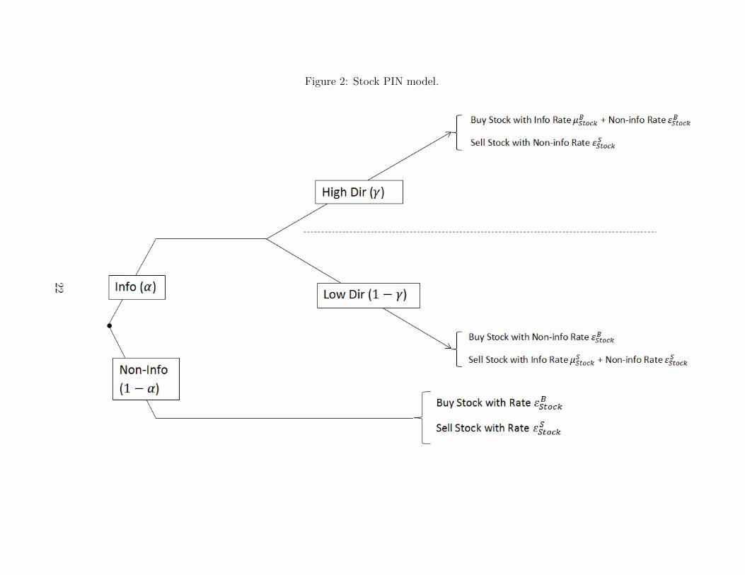
Figure 2: Stock PIN model.
22

Figure 3: Parameter distribution with pooled data in Option PIN model.
This figure provides the empirical distribution of the estimated Option PINmodel parameters with 26 bi-weeks and all the options in our sample. PanelA shows the empirical distribution of Option α, the probability that aninformation event occurs. Panel B shows the empirical distribution of Optionθ, the probability of volatility information happens when information occurs.Panel C shows the empirical distribution of Option δ, the probability of highvolatility information happens when volatility information occurs. Panel Dshows the empirical distribution of Option γ, the probability of high directioninformation happens when direction information occurs. Panel E shows theempirical distribution of Volatility PIN. Panel F shows the empirical distributionof Direction PIN.
Panel A: Empirical distribution of Option α, the probability that an information eventoccurs.
Panel B: Empirical distribution of Option θ, the probability of volatility informationhappens when information occurs.
23

Panel C: Empirical distribution of Option δ, the probability of high volatility informationhappens when volatility information occurs.
Panel D: Empirical distribution of Option γ, the probability of high direction informationhappens when direction information occurs.
24

Panel E: Empirical distribution of Volatility PIN.
Panel F: Empirical distribution of Direction PIN.
25

Figure 4: Parameter distribution with pooled data in Stock PIN model.
This figure provides the empirical distribution of the estimated Stock PIN modelparameters with 26 bi-weeks and all the options in our sample. Panel A showsthe empirical distribution of Stock α, the probability that an information eventoccurs. Panel B shows the empirical distribution of Stock γ, the probabilityof good news happens when information occurs. Panel C shows the empiricaldistribution of Stock PIN.
Panel A: Empirical distribution of Stock α, the probability that an information event occurs.
Panel B: Empirical distribution of Stock γ, the probability of good news happens wheninformation occurs.
26

Panel C: Empirical distribution of Stock PIN.
27

Figure 5: Percentage Changes in Information Measures Around Earning Announcement.
28

Table 1: Finite sample properties of the MLE estimators of the Option PIN model based onMonte Carlo Simulations
The finite sample properties are based on 200 replications of either 100 or 300observation days, that is, 100 or 300 sets of number of long call, short call, longput and short put orders. NC is the number of replications for which the opti-mization converged to feasible estimates, MEAN is the mean estimates, whichis calculated by MEAN = 1
NC
∑NCi=1 η̂i, and SEM is the standard error of the
MEANs, which is calculated by SEM = 1√NC
[ 1(NC−1)
∑NCi=1(η̂i −MEAN)2]1/2,
where η ∈ {α, δ, θ, γ, ε, µ, ν}.T = 100 T = 300
Set Parameter Sim Val NC Mean SEM NC Mean SEM1 α 0.50 200 0.494 0.048 200 0.501 0.031
θ 0.50 200 0.491 0.074 200 0.500 0.043δ 0.50 200 0.503 0.103 200 0.502 0.062γ 0.50 200 0.496 0.100 200 0.500 0.057ε 100.00 200 100.063 0.612 200 100.012 0.340µ 100.00 200 100.291 2.162 200 100.035 1.157ν 100.00 200 99.877 2.127 200 100.004 1.183
2 α 0.50 200 0.506 0.051 200 0.501 0.030θ 0.50 200 0.497 0.070 200 0.495 0.038δ 0.50 200 0.509 0.105 200 0.504 0.056γ 0.50 200 0.498 0.092 200 0.495 0.063ε 100.00 200 99.911 0.559 200 99.971 0.353µ 50.00 200 50.108 1.808 200 50.046 1.169ν 50.00 200 50.200 1.827 200 49.990 1.131
3 α 0.30 200 0.299 0.046 200 0.298 0.025θ 0.70 200 0.704 0.088 200 0.702 0.049δ 0.50 200 0.493 0.114 200 0.497 0.065γ 0.50 200 0.498 0.173 200 0.500 0.093ε 100.00 200 99.960 0.567 200 99.996 0.310µ 100.00 200 100.174 2.261 200 99.914 1.296ν 100.00 200 100.148 3.687 200 99.991 2.019
4 α 0.30 200 0.295 0.049 200 0.298 0.026θ 0.70 200 0.696 0.085 200 0.699 0.046δ 0.40 200 0.388 0.103 200 0.402 0.061γ 0.40 200 0.405 0.177 200 0.397 0.098ε 100.00 200 99.969 0.547 200 100.005 0.324µ 100.00 200 99.870 2.287 200 100.025 1.339ν 100.00 200 100.104 3.508 200 100.201 2.079
5 α 0.30 200 0.301 0.051 200 0.300 0.025θ 0.70 200 0.702 0.086 200 0.702 0.047δ 0.40 200 0.403 0.108 200 0.401 0.060γ 0.40 200 0.393 0.178 200 0.395 0.100ε 50.00 200 49.726 3.484 200 49.989 0.216µ 100.00 200 100.252 1.902 200 99.893 1.066ν 100.00 200 99.796 4.385 200 99.897 1.738
6 α 0.30 200 0.299 0.086 200 0.301 0.029θ 0.70 200 0.681 0.143 200 0.704 0.047δ 0.40 200 0.402 0.154 200 0.404 0.062γ 0.40 200 0.409 0.193 200 0.401 0.095ε 50.00 200 47.852 9.450 200 49.929 0.852µ 100.00 200 99.427 4.285 200 100.194 2.323ν 150.00 200 146.982 13.883 200 150.218 2.191
29

Table 2: Variable Description for Option
Variable Description Frequency / Estimation Pe-riod
OptionOption Spread ($) Option’s ask price minus bid price from OPRA database Transaction / BiweekOption Rel Spread Option spread divide by the mid-point of the ask bid spread from
OPRA databaseTransaction / Biweek
Log(Option Volume) Natural logarithm of the option volume from OPRA database Transaction / BiweekLog(Daily Option Volume) Natural logarithm of daily average option volume from OPRA
databaseTransaction / Average Daily
∆ The data is from Optionmetrics. ∆ of the option is calculated bythe change in option premium for a $1.00 change in underlying price
Last day of period t
Θ The data is from Optionmetrics. Θ is calculated by the change inoption premium as time passes, in terms of dollars per year.
Last day of period t
V ega The data is from Optionmetrics. Vega is calculated by the changein option premium, in cents, for one percentage point change involatility.
Last day of period t
Γ The data is from Optionmetrics. Γ is calculated by the absolutechange in ∆ for a $1.00 change in underlying price.
Last day of period t
Unpriced Volatility (annu-alized)
Realized Volatility of time period t+ 1 minus Implied volatility atthe last day of time period 1 from Optionmetrics
Biweek
Implied Volatility (annual-ized)
The data is from Optionmetrics. IV is calculated for options withstandard settlement at last day of time period t.
Last day of period t
Realized Volatility (annual-ized)
The data is from Optionmetrics. Biweek at t+ 1
Abs(Unpriced Volatility)(annualized)
Absolute Value of Unpriced Volatility from Optionmetrics Biweek
30
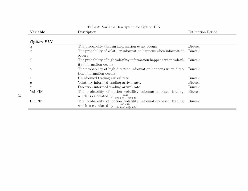
Table 3: Variable Description for Option PIN
Variable Description Estimation Period
Option PINα The probability that an information event occurs Biweekθ The probability of volatility information happens when information
occursBiweek
δ The probability of high volatility information happens when volatil-ity information occurs
Biweek
γ The probability of high direction information happens when direc-tion information occurs
Biweek
ε Uninformed trading arrival rate. Biweekµ Volatility informed trading arrival rate. Biweekν Direction informed trading arrival rate. BiweekVol PIN The probability of option volatility information-based trading,
which is calculated by αθµαθµ+α(1−θ)ν+2ε
Biweek
Dir PIN The probability of option volatility information-based trading,which is calculated by α(1−θ)ν
αθµ+α(1−θ)ν+2ε
Biweek
31

Table 4: Variable Description for Stocks
Variable Description Estimation Period
StockReturn (Per Day) Raw return from CRSP database BiweekS&P 500 Return (Per Day) S&P 500 return from CRSP database BiweekExcess Return (Per Day) Raw return minus S&P 500 Return from CRSP database BiweekStock Spread ($) Stock ask price minus bid price from CRSP database BiweekStock Rel Spread Stock ask bid spread divide by mid-point of ask and bid price from
CRSP databaseBiweek
Log(Daily Stock Volume) Natural logarithm of biweek daily stock volume from CRSPdatabase
Average Daily
Log(Market Cap) Natural logarithm of market capital at last day of period t fromCRSP database
Last day of period t
Stock PINStock α The probability that an information event occurs. BiweekStock δ The probability of good news happens when information occurs. BiweekStock ε Uninformed trading arrival rate. BiweekStock µ Informed trading arrival rate. BiweekStock PIN The probability of stock information-based trading, which is calcu-
lated by Stock δ∗Stock µStock δ∗Stock µ+2Stock ε
.Biweek
32

Table 5: Summary Statistics for Options
Variable Obs Mean Std. Dev. Min Max
OptionOption Ask Bid Spread ($) 8062 0.105 0.310 0.014 2.947
Option Rel Ask Bid Spread (%) 8062 5.8 4.3 1.5 23Log(Option Volume) 8056 10.485 1.263 8.350 14.097
Log(Daily Option Volume) 8056 8.219 1.263 6.084 11.841
∆ 7994 0.526 0.016 0.508 0.615Θ 7994 -12.981 12.866 -83.370 -1.594
V ega 7994 5.909 5.744 0.534 39.047Γ 7994 0.137 0.109 0.012 0.613
Unpriced Volatility 7993 -0.013 0.154 -0.631 0.917Implied Volatility 7994 0.390 0.171 0.128 1.010
Realized Volatility 7995 0.377 0.223 0.081 1.265Abs(Unpriced Volatility) 7993 0.104 0.115 0.000 0.917
Option PINα 8064 0.457 0.064 0.066 0.838θ 8064 0.491 0.114 0.023 0.989δ 8064 0.613 0.203 0.013 0.988γ 8064 0.485 0.176 0.013 0.988ε 8064 158.939 876.544 4.731 27345.970µ 8064 372.193 1267.470 10.783 35709.450ν 8064 303.602 1048.574 11.013 33978.800
Vol PIN 8064 0.225 0.066 0.091 0.410Dir PIN 8064 0.202 0.066 0.078 0.396
33

Table 6: Summary Statistics for Stocks
Variable Obs Mean Std. Dev. Min Max
StockReturn (%) 8029 -0.03 0.74 -2.42 1.96
S&P 500 Return (%) 8029 -0.0044 0.303 -0.85 0.71Excess Return (%) 8029 -0.03 0.64 -2.20 1.76
Stock Ask Bid Spread ($) 8030 0.0164 0.0202 0.0089 0.1720Stock Rel Ask Bid Spread (%) 8030 0.045 0.038 0.010 0.231
Log(Daily Stock Volume) 8036 15.547 0.971 13.249 18.248Log(Mkt Cap) 8030 16.306 1.412 12.893 19.161
Stock PINStock α 8050 0.338972 0.049538 0.167751 0.574098Stock δ 8050 0.490051 0.177726 0.041407 0.928179Stock ε 8050 288674.3 642479.7 3491.761 16900000Stock µ 8050 342090.1 825344.1 6671.03 24400000
Stock PIN 8050 0.169494 0.032986 0.113421 0.28505
34

Table 7: Correlation MatrixDirPIN
VolPIN
StockPIN
Abs(UV)
ExcessRet
Log(DailyOp-tionVol-ume)
Log(DailyStockVol-ume)
Log(MktCap)
StockRelAskBid
OptionRelAskBid
IV RV IC RC
Dir PIN 1.00Vol PIN -0.05 1.00Stock PIN 0.22 0.09 1.00Abs(Unpriced Vol) 0.04 0.03 0.09 1.00Excess Return 0.02 0.00 -0.01 -0.08 1.00Log(Daily Option Volume) -0.56 -0.40 -0.14 -0.07 -0.01 1.00Log(Daily Stock Volume) -0.29 -0.12 -0.14 -0.06 0.00 0.70 1.00Log(Market Cap) -0.33 -0.11 -0.39 -0.23 0.05 0.42 0.33 1.00Stock Rel Ask Bid 0.22 0.15 0.33 0.19 -0.07 -0.16 0.11 -0.48 1.00Option Rel Ask Bid 0.39 0.22 0.29 -0.01 -0.01 -0.49 -0.30 -0.29 0.25 1.00Implied Vol 0.06 -0.02 0.03 0.33 -0.07 -0.13 0.03 -0.53 0.46 -0.11 1.00Realized Vol 0.05 -0.02 0.01 0.54 -0.11 -0.08 0.03 -0.38 0.32 -0.11 0.72 1.00IC -0.10 -0.16 0.05 0.02 0.01 0.02 -0.25 0.02 0.09 -0.01 0.03 0.01 1.00RC -0.09 -0.17 0.06 0.02 0.01 0.00 -0.27 0.01 0.10 0.00 0.03 0.01 0.98 1.00
35

Table 8: Sort by Market Cap
Log(MktCap) Log(Stock Vol) Log(Option Vol) VolPIN DirPIN StockPIN1 (Low) 14.215 15.265 7.727 0.230 0.226 0.190
2 15.605 15.266 7.784 0.236 0.220 0.1773 16.367 15.440 8.045 0.224 0.204 0.1664 17.157 15.535 8.182 0.227 0.198 0.159
5 (High) 18.184 16.234 9.330 0.210 0.162 0.156(1-5) -3.97 -.969 -1.603 0.020 0.0642 0.034
(-190.020) (-30.171) (-41.95) (8.815) (29.672) (29.437)
36

Table 9: Regression on Abs(Unpriced Volatility)
This table reports the coefficients from fixed effect panel regression of absoluteunpriced volatility. The absolute unpriced volatility is defined as the t − 1 pe-riod last day implied volatility (IV) minus the t period realized volatility (10days). VolPIN is the probability of option volatility information-based trading instock/option i of biweek t− 1, which is calculated by αθµ
αθµ+α(1−θ)ν+2εand DirPIN
is the probability of option volatility information-based trading in stock/option
i of biweek t− 1, which is calculated by α(1−θ)ναθµ+α(1−θ)ν+2ε
. The dummy is defined to
be 1 if IV>Realized Volatility(RV), 0 otherwise. Log(Market Cap) is the naturallogarithm of t−1 period last price times total shares outstanding. Log(Daily Op-tion Volume) is the natural logarithm of t−1 period daily average option volume.All the variables are winsorized at 1% level. Time and firm effects are controlledand s.e. is adjusted using robust option. T-stat is reported in parentheses with*** p < 0.01, ** p < 0.05, * p < 0.1.
(1) (2) (3) (4) (5)
VolPIN 0.113*** 0.222*** 0.120*** 0.227*** 0.199***(4.191) (7.399) (3.899) (6.863) (4.620)
I(IV > RV )*VolPIN -0.171*** -0.172*** -0.131***(-14.83) (-14.95) (-4.129)
DirPIN 0.0579** 0.0447 0.0695** 0.0541* 0.0871**(2.096) (1.632) (2.198) (1.736) (2.034)
I(IV > RV )*DirPIN -0.0498(-1.448)
Log(Market Cap) -0.0366*** -0.0368*** -0.0369***(-4.823) (-4.889) (-4.899)
Log(Daily Option Volume) 0.00861*** 0.00819*** 0.00824***(3.088) (2.959) (2.983)
Constant 0.0664*** 0.0697*** 0.588*** 0.599*** 0.601***(6.578) (6.959) (4.701) (4.828) (4.836)
Time Effect YES YES YES YES YESFirm Effect YES YES YES YES YES
Observations 7,993 7,993 7,956 7,956 7,956R-squared 0.002 0.033 0.006 0.038 0.038
No. of Tickers 481 481 479 479 479
37

Table 10: Asset Pricing Test
This table reports the average coefficients of Fama-MacBeth (1973) regression of the (daily) excess return ofstock. Rit = γ0t + γ1tβ̂p + γ2tStockPINit−1 + γ3tV olPINit−1 + γ4tDirPINit−1 + γ5tSIZEit−1 + γ6tYit−1 + ηit,
where Rit is the excess return of stock i in biweek t; β̂p is the portfolio betas calculated from the full periodusing 20 sorted portfolios; StockPINit−1 is the probability of information-based trading in stock i of biweekt− 1, which is calculated by Stock δ∗Stock µ
Stock δ∗Stock µ+2Stock ε; VolPIN is the probability of option volatility information-
based trading in stock/option i of biweek t − 1, which is calculated by αθµαθµ+α(1−θ)ν+2ε
and DirPIN is the
probability of option direction information-based trading in stock/option i of biweek t−1, which is calculated
by α(1−θ)ναθµ+α(1−θ)ν+2ε
; SIZEit−1 is the natural logarithm of market value of equity in firm i at the end of biweek
t − 1, Yit−1 is other control variables. Robust Newey-West (1987) adjusted t-stat is reported in parentheseswith *** p < 0.01, ** p < 0.05, * p < 0.1.
(1) (2) (3) (4) (5) (6) (7)
Portfolio β*104 -0.03 -0.012 -0.99 -1.42 -1.08 -1.03 -1.02(-0.00641) (-0.000) (-0.227) (-0.314) (-0.234) (-0.241) (-0.251)
Stock PIN*103 1.372 0.274(0.28) (0.0496)
VolPIN*103 1.13 1.68 0.815 1.39 1.03(0.668) (1.067) (0.442) (0.742) (0.587)
DirPIN*103 3.80** 3.98** 3.14* 4.17** 3.62*(2.384) (2.624) (1.827) (2.392) (1.901)
Log(Market Cap)*104 1.88*** 1.97** 2.50*** 1.49* 1.25 2.86*** 2.44***(3.308) (2.564) (3.604) (1.894) (1.442) (2.866) (3.323)
Stock Rel Ask Bid Spread*102 -0.757*(-1.960)
Implied Vol -0.00216**(-2.225)
Turnover*105 6.63(0.929)
Constant -0.00337*** -0.00378* -0.00528*** -0.00341 -0.00227 -0.00617** -0.00519***(-3.191) (-2.176) (-2.944) (-1.628) (-0.875) (-2.559) (-3.144)
Observations 8,029 8,024 8,029 8,029 7,964 8,029 8,024R-squared 0.035 0.043 0.050 0.061 0.094 0.055 0.058
Number of groups 26 26 26 26 26 26 26
38

Table 11: Asset Pricing Test (FE Panel Regression)
This table reports the coefficients of fixed effect panel regression of the (daily) excess return of stock. Rit =γ0t + γ1tβ̂p + γ2tStockPINit−1 + γ3tV olPINit−1 + γ4tDirPINit−1 + γ5tSIZEit−1 + γ6tYit−1 + ηit, where Rit
is the excess return of stock i in biweek t, β̂p is the portfolio betas calculated from the full period using20 sorted portfolios; StockPINit−1 is the Stock PIN, the probability of information-based trading in stocki of biweek t − 1, which is calculated by Stock δ∗Stock µ
Stock δ∗Stock µ+2Stock ε; VolPIN is the probability of option volatility
information-based trading in stock/option i of biweek t− 1, which is calculated by αθµαθµ+α(1−θ)ν+2ε
and DirPIN
is the probability of option direction information-based trading in stock/option i of biweek t − 1, which is
calculated by α(1−θ)ναθµ+α(1−θ)ν+2ε
; SIZEit−1 is the natural logarithm of market value of equity in firm i at the end
of biweek t− 1, Yit−1 is other control variables. All the variables are winsorized at 1% level. Time and firmeffects are controlled and s.e. is adjusted using robust option. T-stat is reported in parentheses with ***p < 0.01, ** p < 0.05, * p < 0.1.
(1) (2) (3) (4) (5) (6) (7)
Portfolio β*104 -5.05 -4.92 4.85 -5.13 -3.78 -4.40 -4.73(-0.855) (-0.826) (-0.819) (-0.870) (-0.644) (-0.745) (-0.795)
Stock PIN*103 7.93*** 7.41**(2.692) (2.509)
VolPIN*103 1.74 1.78 1.77 1.06 1.53(1.015) (1.029) (1.028) (0.590) (0.886)
DirPIN*103 5.18*** 5.20*** 4.62*** 4.43** 4.89***(3.097) (3.102) (2.727) (2.520) (2.915)
Log(Market Cap)*104 -50.1*** -50.3*** -47.9*** -50.1*** -71.2*** -50.1*** -48.2***(-8.976) (-8.860) (-8.708) (-7.846) (-10.27) (-8.789) (-8.612)
Stock Rel Ask Bid Spread*102 -0.614(-0.853)
Implied Vol -0.00606***(-6.733)
Turnover*105 -43.6*(-1.753)
Constant 0.0819*** 0.0808*** 0.0769*** 0.0807*** 0.117*** 0.0820*** 0.0763***(8.937) (8.692) (8.441) (7.542) (10.01) (8.421) (8.238)
Observations 8,029 8,024 8,029 8,029 7,964 8,029 8,024R-squared 0.021 0.022 0.023 0.023 0.031 0.023 0.023
No. of Tickers 483 483 483 483 479 483 483
39

Table 12: Regression on Option Rel Ask Bid Spread
This report reports the coefficients from OLS and fixed effect panel regression of option relative ask bidspread. The option relative ask bid spread is defined as the option ask bid spread divide by the average quoteprice (ask+bid
2); Stock PIN is the probability of information-based trading in stock i of biweek t− 1, which is
calculated by Stock δ∗Stock µStock δ∗Stock µ+2Stock ε
; VolPIN is the probability of option volatility information-based trading in
stock/option i of biweek t− 1, which is calculated by αθµαθµ+α(1−θ)ν+2ε
and DirPIN is the probability of option
direction information-based trading in stock/option i of biweek t − 1, which is calculated by α(1−θ)ναθµ+α(1−θ)ν+2ε
;
Initial hedging cost (IC) is the cost to set up a delta neutral position by purchasing ∆ shares of the stockat the ask price and close the position by selling at the bid price, which is calculated by kS∆; Rebalancehedging cost is calculated by νk; Log(Daily Option Volume) is the natrual logarithm of the average dailyoption volume at biweek t. Time and firm effects are controlled and s.e. is adjusted using robust option.T-stat is reported in parentheses with *** p < 0.01, ** p < 0.05, * p < 0.1.
(1) (2) (3) (4) (5) (6)
VolPIN 0.0517*** 0.0513*** 0.0516*** 0.0164*** 0.0164*** 0.0165***(6.646) (6.309) (6.294) (2.608) (2.601) (2.610)
DirPIN 0.111*** 0.110*** 0.110*** 0.0194*** 0.0195*** 0.0196***(11.82) (11.44) (11.44) (2.919) (2.917) (2.924)
Stock PIN 0.266*** 0.261*** 0.261*** 0.0698*** 0.0713*** 0.0713***(17.75) (17.19) (17.14) (5.504) (5.561) (5.565)
IC 0.0516** -0.0589**(2.444) (-2.143)
RC 0.286** -0.144(2.361) (-0.914)
Log(Daily Option Volume) -0.0113*** -0.0112*** -0.0112*** -0.00404*** -0.00401*** -0.00402***(-23.56) (-22.63) (-22.44) (-4.490) (-4.390) (-4.402)
Constant 0.0720*** 0.0717*** 0.0714*** 0.0719*** 0.0717*** 0.0716***(10.78) (10.37) (10.25) (7.512) (7.480) (7.459)
Time Effect NO NO NO YES YES YESFirm Effect NO NO NO YES YES YES
Observations 8,041 7,952 7,952 8,041 7,952 7,952R-squared 0.308 0.304 0.304 0.032 0.033 0.033
No. of Tickers 485 479 479
40

Table 13: Event Study on DirPIN, VolPIN, Stock PIN and Rel Ask Bid
This table reports the coefficients from fixed effect panel regression of the infor-mation measures. The information measures include DirPIN, VolPIN, Stock PINand Option Rel Spread. We only keep the data for biweek t−2, t−1, t, t+1, t+2,where t is the biweek with an earning announcement; Stock PIN is the prob-ability of information-based trading in stock i of biweek t − 1, which is cal-culated by Stock δ∗Stock µ
Stock δ∗Stock µ+2Stock ε; VolPIN is the probability of option volatility
information-based trading in stock/option i of biweek t−1, which is calculated byαθµ
αθµ+α(1−θ)ν+2εand DirPIN is the probability of option direction information-based
trading in stock/option i of biweek t − 1, which is calculated by α(1−θ)ναθµ+α(1−θ)ν+2ε
;option relative ask bid spread is defined as the option ask bid spread divide bythe average quote price (ask+bid
2); Pre-Earning Dummy is defined as 1 if the next
biweek has an earning announcement, 0 otherwise; Earning Dummy is defined as1 if the biweek has an earning announcement, 0 otherwise; Post-Earning Dummyis defined as 1 if the previous biweek has an earning announcement, 0 otherwise.We control the option greeks for the regressions with dependent variables DirPIN,VolPIN and Option Rel Ask Bid Spread. Time and firm effects are controlledand s.e. is adjusted using robust option. T-stat is reported in parentheses with*** p < 0.01, ** p < 0.05, * p < 0.1.
(1) (2) (3) (4)Variables DirPIN VolPIN Stock PIN Option Rel Ask Bid Spread
Pre-Earning Dummy -0.00121 -0.00130 0.00298*** -0.00182***(-0.607) (-0.641) (3.285) (-2.920)
Earning Dummy -0.0130*** -0.00636*** 0.00307*** -0.00345***(-6.709) (-3.217) (3.473) (-5.687)
Post-Earning Dummy -0.00246 -0.00435** -0.00387*** 0.00214***(-1.246) (-2.169) (-4.299) (3.475)
Constant 0.160*** 0.219*** 0.166*** 0.0673***(5.575) (7.485) (313.1) (7.479)
Control for Option Greeks YES YES NO YESTime Effect YES YES YES YESFirm Effect YES YES YES YES
Observations 5,361 5,361 5,358 5,361R-squared 0.015 0.016 0.012 0.145
Number of Tickers 412 412 411 412
41