vol. no. asymptotic waveform evaluation for timing...

352 IEEE TRANSACTIONS ON COMPUTER-AIDED DESIGN. VOL. 9. NO. 4. APRIL I990

Asymptotic Waveform Evaluation for Timing Analysis

LAWRENCE T. PILLAGE, MEMBER, IEEE, A N D RONALD A. ROHRER, FELLOW, I E E ~

Abstract-For digital system designs the propagation delays due to the physical interconnect can have a significant, even dominant, impact on performance. Timing analyzers attempt to capture the effect of the interconnect on the delay with a simplified model, typically an RC tree. For mid-frequency MOS integrated circuits the RC tree methods can predict the delay to within 10 percent of a SPICE simulation and at faster than lOOOx the speed. With continual progress in integrated circuit processing, operating speeds and new technologies are emerging that may require more elaborate interconnect models. Digital bipolar and high-speed MOS integrated systems can require interconnect models which contain coupling capacitors and inductors. In addition, to enable timing verification at the printed circuit hoard level also requires general RLC interconnect models. Asymptotic Waveform Eval- uation (AWE) provides a generalized approach to linear RLC circuit response approximations. The RLC interconnect model may contain floating capacitors, grounded resistors, inductors, and even linear controlled sources. The transient portion of the response is approximated by matching the initial boundary conditions and the first 2q-1 moments of the exact response to a lower order q-pole model. For the case of an RC tree model a first-order AWE approximation reduces to the RC tree methods.

I. INTRODUCTION ITH FINER feature sizes and higher signal speeds, systems that are designed to be digital may evi-

dence aspects of analog behavior in their interconnect, which become the ultimate determinants of performance. Timing analyzers [ 11-[4] and timing simulators [5], 161 attempt to capture the effect of the interconnect on the delay to produce reliable timing verification. For many MOS circuits, timing analyzers [ 11, [3] are often able to predict the interconnect delay with a simplified model, typically an RC tree [7], to within 10 percent of a SPICE [8] simulation prediction. RC trees are RC circuits with capacitors from all nodes to ground, no floating capacitors, no resistor loops, and no resistors to ground. The signal delays through an RC tree are often estimated using a form of the Elmore delay [9], which provides a dominant time constant approximation for monotonic step responses.

To enable the timing verification of bipolar circuits, the

Manuscript received September 6, 1988; revised April 24, 1989. This work was supported in part by Digital Equipment Corporation and the Semiconductor Research Corporation. This paper was recommended by Associate Editor R. K . Brayton.

L. T. Pillage is with the Department of Electrical and Computer Engi- neering, The University of Texas at Austin, Austin, TX 78712.

R. A. Rohrer is with the Department of Electrical and Computer Engi- neering, Carnegie Mellon University, Pittsburgh, PA 15213.

IEEE Log Number 8933519.

interconnect model may need to include grounded resistors [ 101 and inductors [ 1 11 which are not compatible with RC trees. Even for MOS circuits at particularly high speeds, the effects of coupling capacitance may need to be included in the delay estimate. Particularly at the printed circuit board level, input voltage rise time can dominate the timing of a net thus precluding the use of step response approximations for delay estimation. More- over, for generality, a solution is required when there are nonequilibrium initial conditions so that the delays due to charge sharing effects can be predicted.

RLC circuits with nonequilibrium initial conditions may have response waveforms which are nonmonotonic. A single time constant approximation with the Elmore delay is not generally applicable for such circuits. Two time constant models have been shown to improve the accuracy [12], where they too have been applied to RC tree monotone response approximations. Asymptotic Wave- form Evaluation (AWE) provides a generalized approach to waveform estimation for RLC circuits with initial conditions and nonzero input signal risetimes. The RLC circuits may contain floating capacitors, grounded resistors, inductors, and linear controlled sources. The transient response of an RLC circuit is approximated by matching the initial boundary conditions and the first 2q-1 moments of the actual response to a lower order q-pole model. For the case of an RC tree driven by a step input, a first-order AWE approximation is equivalent to the methods which employ Elmore’s delay expression.

Section I1 begins with a discussion of previous work in delay estimation for timing analysis. The RC tree methods which employ Elmore’s delay expression are briefly reviewed. For a more detailed summary of the previous work refer to [ I 11. Next, AWE is described in general in terms of state variable analysis. The state variable for- mulation is used only to explain AWE as applied in general to RLC circuits. Then in Section IV the practical pro- cedural steps of AWE are described and related to the RC tree methods. Finally, examples of AWE are provided for a variety of RLC interconnect circuit models, followed by our concluding remarks in Section VI.

11. RC TREE METHODS A typical approach to timing analysis of MOS inte-

grated circuits is to divide the design into stages, with each stage consisting of a gate output and the interconnect

0278-0070/90/0400-0352$01 .OO @ 1990 IEEE

Authorized licensed use limited to: Michigan Technological University. Downloaded on October 29, 2009 at 12:29 from IEEE Xplore. Restrictions apply.

PILLAGE A N D ROHRER: WAVEFORM EVALUATION FOR TIMING ANALYSIS 353

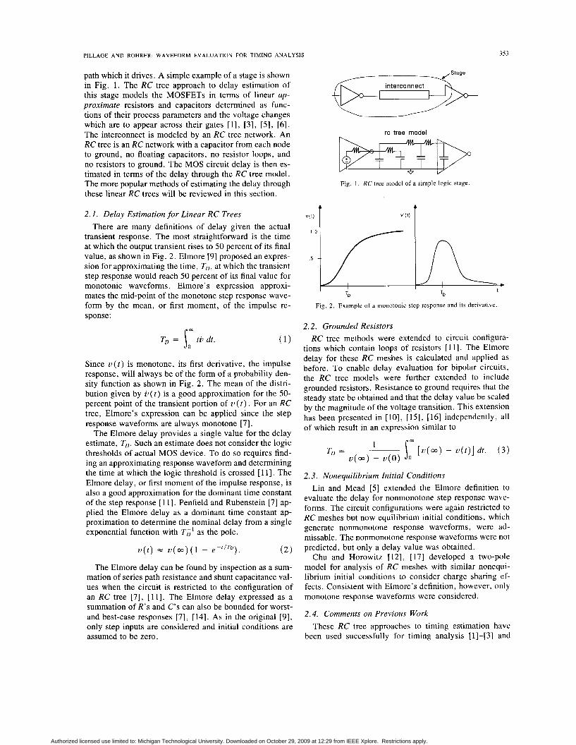
path which it drives. A simple example of a stage is shown in Fig. 1. The RC tree approach to delay estimation of this stage models the MOSFETs in terms of linear approximate resistors and capacitors determined as functions of their process parameters and the voltage changes which are to appear across their gates [ l l , [3l, [5l, [6l. The interconnect is modeled by an RC tree network. An RC tree is an RC network with a capacitor from each node to ground, no floating capacitors, no resistor loops, and no resistors to ground. The MOS circuit delay is then estimated in terms of the delay through the RC tree model. The more popular methods of estimating the delay through these linear RC trees will be reviewed in this section.

2.1. Delay Estimation for Linear RC Trees There are many definitions of delay given the actual

transient response. The most straightforward is the time at which the output transient rises to 50 percent of its final value, as shown in Fig. 2. Elmore [9] proposed an expression for approximating the time, TD, at which the transient step response would reach 50 percent of its final value for monotonic waveforms. Elmore’s expression approximates the mid-point of the monotone step response waveform by the mean, or first moment, of the impulse response:

W

To = tu dt. (1)

Since v ( t ) is monotone, its first derivative, the impulse response, will always be of the form of a probability den- sity function as shown in Fig. 2. The mean of the distri- bution given by i, ( t ) is a good approximation for the 50- percent point of the transient portion of U ( t ) . For an RC tree, Elmore’s expression can be applied since the step response waveforms are always monotone [7].

The Elmore delay provides a single value for the delay estimate, To. Such an estimate does not consider the logic thresholds of actual MOS device. To do so requires finding an approximating response waveform and determining the time at which the logic threshold is crossed [l 13. The Elmore delay, or first moment of the impulse response, is also a good approximation for the dominant time constant of the step response [ 1 11. Penfield and Rubenstein [7] applied the Elmore delay as a dominant time constant approximation to determine the nominal delay from a single exponential function with T i ‘ as the pole.

u ( t ) = v ( w ) ( 1 - e P r l T D ) . ( 2 )

The Elmore delay can be found by inspection as a summation of series path resistance and shunt capacitance values when the circuit is restricted to the configuration of an RC tree [7], [ l l ] . The Elmore delay expressed as a summation of R’s and C’s can also be bounded for worst- and best-case responses [7], [14]. As in the original [9], only step inputs are considered and initial conditions are assumed to be zero.

interconnect

rc tree model

Fig. 1 . RC tree model of a simple logic stage

+ 4

v ( t ’ I

Fig. 2. Example of a monotonic step response and its derivative.

2.2. Grounded Resistors RC tree methods were extended to circuit configura-

tions which contain loops of resistors [ 111. The Elmore delay for these RC meshes is calculated and applied as before. To enable delay evaluation for bipolar circuits, the RC tree models were further extended to include grounded resistors. Resistance to ground requires that the steady state be obtained and that the delay value be scaled by the magnitude of the voltage transition. This extension has been presented in [lo], [15], [16] independently, all of which result in an expression similar to

2.3. Nonequilibrium Initial Conditions Lin and Mead [ 5 ] extended the Elmore definition to

evaluate the delay for nonmonotone step response waveforms. The circuit configurations were again restricted to RC meshes but now equilibrium initial conditions, which generate nonmonotone response waveforms, were ad- missable. The nonmonotone response waveforms were not predicted, but only a delay value was obtained.

Chu and Horowitz [12], [17] developed a two-pole model for analysis of RC meshes with similar nonequilibrium initial conditions to consider charge sharing effects. Consistent with Elmore’s definition, however, only monotone response waveforms were considered.

2.4. Comments on Previous Work These RC tree approaches to timing estimation have

been used successfully for timing analysis [1]-[3] and


354 lEEE TRANSACTIONS ON COMPUTER-AIDED DESIGN, VOL. 9. NO. 4. APRIL 1Y90

timing simulation [5], [6] of low- to mid-frequency MOS digital integrated circuits. The single time-constant and double time-constant models provide good delay esti- mates for RC tree paths when driven by step inputs; higher order approximations may be required, however, when inductance and floating capacitance effects are not negli- gible. Although nonequilibrium initial conditions are considered for the one- and two-pole models, they are valid for a limited set of conditions and may be unable to provide a means of handling the nonmonotone waveforms which may result in general.

111. ASYMPTOTIC WAVEFORM EVALUATION (AWE) Timing analysis of more general digital circuits may

require models more elaborate than RC trees driven by single step inputs. Analysis of RLC interconnect circuit models with initial conditions and nonmonotone response waveforms requires a more comprehensive waveform es- timator. AWE is a generalized approach to approximating the waveform response of linear circuits with multiple step and ramp input signals and unrestricted nonequilibrium initial conditions.

3.1. The A WE Approximation AWE is most conveniently explained in general in terms

of the differential state equations for a lumped, linear, time-invariant circuit:

x = A x + B u (4 1 where x is the n-dimensional state vector and U is the m- dimensional excitation vector. In all but the most patho- logical cases such a circuit description exists [ 181. Once AWE is explained in general, the results will be particu- larized to the more familiar RC tree circuits for comparison with the present practices of delay estimation from the previous section.

Suppose that the particular excitation is of the form

up(t) = uo + u , t , t I to ( 5 ) where uo and u I are constant m-dimensional vectors. In general the form of up ( t ) need not be confined to such simple signals, but rather could assume any form of input excitation for which a particular solution can easily be obtained. Inputs that are polynomials in time or sums of complex-valued exponentials can in theory be as easily accommodated as the step/ramp combination in expression ( 5 ) . For present purposes this simple class of input excitations is considered because it is adequate for the in- vestigation of delay and rise time effects.

For the excitation up, ( 5 ) , the differential-state equations (4) has the particular solution

xp(t) = -A-'Buo - AP2BuI - A - ' B u I t . (6)

The A-matrix may not be singular for this particular solution to exist. This condition is equivalent to specifying that the circuit in question have a unique and well-defined dc solution when all of its capacitances are open-circuited and all of its inductances are short-circuited. This is not

an unreasonable restriction for most of the circuits for which delay estimation may be of interest. There are situations, however, when a node is isolated such that it is connected to the supply voltage only through capacitors. The steady-state solution for these floating nodes must be determined by the charge conservation equation. Assum- ing for now that there are no floating nodes in the circuit, we complete the solution of (4) with the homogeneous equation:

now with the initial condition

xh = h h (7 )

( 8 ) ~ ~ ( 0 ) = x0 + A - I B U ~ + A - ~ B U ~

xh(S) = (SI - A)-IXh(O).

where xo is the initial state at time zero. The Laplace transform solution of the homogeneous equation is

( 9 )

To approximate this solution, x h ( s ) is first expanded in a Maclaurin series

X ~ ( S ) = -A-I(Z + A-lS + AP2S2 + . * * ) xh(0)

( 10) and as many moments as necessary or desirable are matched in terms of lower order approximating functions. The justification for such a moment matching approach follows from the Laplace transform definition

I-" " . P" 1

X(s) = lo e-sfx( t ) dt = c - ( - s ) ~ 1 tkx(t ) dt k = O k! 0

since it has long been established that the time moments:

provide excellent measures of delays, rise times, etc. [9], [ 191. Focusing for now on a specific component of xh (s ) , say the ith, its initial conditions and first 2q - 1 moments

It is these moments that are matched to a lower order frequency-domain function of the form

kl k2 k4 Z;(s)=-+-+ * * * +- $ - P I s - P 2 s - Py


PILLAGE AND ROHRER: WAVEFORM EVALUATION FOR TIMING ANALYSIS 355

where p I through p q are the complex approximating poles and k l through k9 their appropriate residues. In other words, the time-domain moments are to be matched to those of an approximating function of the form

4

I = I i, ( t ) = c kreP". (15)

Under the assumption that the moments (13) can be generated easily-more on this when computational con- siderations are discussed-what remains now is to solve for the time constants and their corresponding residues. Expanding each of the terms in (14) into a series about the origin, and upon inclusion of the initial conditions, the following set of nonlinear simultaneous equations for the ith state variable is obtained:

- ( k l + k2 + - - a + k q ) = [ m - , ] ,

h

(16) A solution for the approximating poles and residues from this set of nonlinear equations could proceed in terms of Newton-Raphson [20] or a similar iteration method. The complexity of these indirect solution methods, however, is not fixed, but varies with the problem. Moreover, heu- ristics are needed to monitor the iteration step size to control convergence.

Instead of attempting to solve the nonlinear equations given by (16), we will reformulate the problem to allow for direct solution of the approximating poles and residues. The set of equations in (16) can be summarized in matrix form as

- V k = [ m , ] , (17)

V A - q k = [ m h ] , (18) and

where m, represents the low-order moments ( - 1 , 0, . * * , q - 2 ) , mh represents the high-order moments ( q - 1, q, * - , 2q - 2 ) , A-' is a diagonal matrix of the reciprocal complex poles, and V is the well-known Van- dermonde matrix [2 11 :

1

P 1' I! P c2

1

P Z '

P 2-2

. . .

. . .

. . .

1

P q

P q

- I

- 2

It follows then from (17) that

and

Since the Vandermonde matrix is the modal matrix for a system matrix in companion form [ 191, (2 1) is equivalent to

ATqm, = mh ( 2 2 )

where

L - a , -a, -a2 . . .

with the coefficients normalized so that aq = 1. This matrix is characterized as A,' rather than A , because its eigenvalues are the reciprocals of the approximating poles for the original system (4). It is shown in [22] that the set of simultaneous nonlinear equations (22) for the coefficients a, through aq - , , a,, can be written recursively to yield the following set of linear equations:

m - , m, . . - mq-2

m, ml mq- I

m q P 2 m q - l m 2 q - 3 -

(24)

It is in terms of a, that we can form a characteristic polynomial

a, + a l p - ' + a 2 p - 2 + * * * + a 9 - I p - 9 + 1 + p - 9 = O

( 2 5 )

the roots of which are the reciprocals of the desired poles. If the poles are not distinct, the Vandermonde matrix is

by definition singular. For such cases the residues must be found using an expression other than (20). For the case of a double pole given a second-order approximation:

Expanding the terms in (26) into a series about s = 0:

) 2 ( s ) = $ ( l + - + , + , + 2s 3s2 4s3 - . *

PI PI PI PI


356 I E E E TRANSACTIONS ON COMPUTER-AIDED DESIGN. VOL 9. NO 4. A P R I L 1990

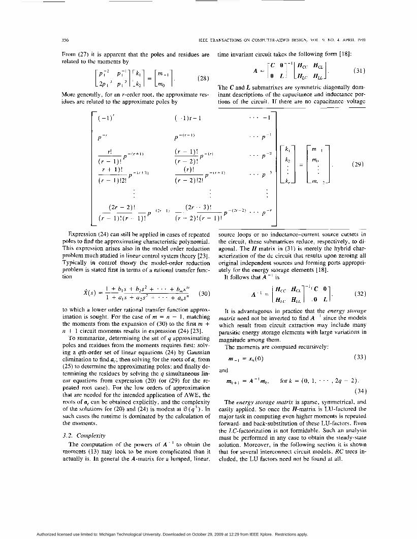
From (27) it is apparent that the poles and residues are time invariant circuit takes the following form [IS]: related to the moments by

The C and L submatrixes are symmetric diagonally dom- More generally, for an r-order root, the approximate residues are related to the approximate poles by

inant descriptions of the capacitance and inductance por- tions of the circuit. If there are no capacitance-voltage

- - 1 r ( - 1 ) r - 1 . . . ( - o r

- 1 P - r P - ( - I ) * * * P

( r - l ) ! ( r - 2 ) !

p - ( r + l ) ~ - ( r ) r!

( r - I ) ! -2

* * P

- 3 P

P - r

(2r - 3 ) ! - ( Z r - 2 ) . . . P - ( 2 r - l )

(2r - 2 ) ! P

( r - l ) ! ( r - l ) ! ( r - 2 ) ! ( r - l ) ! - L

Expression (24) can still be applied in cases of repeated poles to find the approximating characteristic polynomial. This expression arises also in the model order reduction problem much studied in linear control system theory [23]. Typically in control theory the model-order reduction problem is stated first in terms of a rational transfer function

(30) 1 + b l s + b2s2 + . + b,sm X ( s ) = 1 + a ,s + a 2 s 2 + * * + a,s”

to which a lower order rational transfer function approximation is sought. For the case of m = n - 1 , matching the moments from the expansion of (30) to the first m + n + 1 circuit moments results in expression (24) [23].

To summarize, determining the set of q approximating poles and residues from the moments requires first: solving a qth-order set of linear equations (24) by Gaussian elimination to find a,; then solving for the roots of a, from (25) to determine the approximating poles; and finally determining the residues by solving the q simultaneous linear equations from expression (20) (or (29) for the repeated root case). For the low orders of approximation that are needed for the intended application of AWE, the roots of a, can be obtained explicitly, and the complexity of the solutions for (20) and (24) is modest at (3 ( q 3 ) . In such cases the runtime is dominated by the calculation of the moments.

3.2. Complexity The computation of the powers of A - ’ to obtain the

moments (13) may look to be more complicated than it actually is. In general the A-matrix for a lumped, linear,

source loops or no inductance-current source cutsets in the circuit, these submatrices reduce, respectively, to diagonal. The H matrix in (31) is merely the hybrid char- acterization of the dc circuit that results upon zeroing all original independent sources and forming ports appropri- ately for the energy storage elements [ 181.

It follows that A - I is

It is advantageous in practice that the energy storage matrix need not be inverted to find A - I since the models which result from circuit extraction may include many parasitic energy storage elements with large variations in magnitude among them.

The moments are computed recursively:

m-, = x h ( 0 ) (33)

and

m k + l = A - ’ m k , fork = (0, 1 , * , 2q - 2 ) .

( 3 4 ) The energy storage matrix is sparse, symmetrical, and

easily applied. So once the H-matrix is LU-factored the major task in computing even higher moments is repeated forward- and back-substitution of these LU-factors. Even the LC-factorization is not formidable. Such an analysis must be performed in any case to obtain the steady-state solution. Moreover, in the following section it is shown that for several interconnect circuit models, RC trees included, the LU factors need not be found at all.



3.3. Stability Expression (24) is one of many alternative moment

matching methods that may be employed to obtain the approximating poles [23]-[26]. AWE differs from those of control system theory in that the zeros are not found directly, but rather the residues are obtained in order to approximate the time response. More importantly, AWE differs in that the particular solution is subtracted a priori and only the transient portion of the response is approximated. By focusing on the residues and the homogeneous response, the lower order approximation can be forced to match the initial state, m - I , and the finite integral of the voltage response, mo. Since the integral of the approximating voltage waveform is finite and equal to the exact, the final value must also match that of the exact, thus stability in guaranteed.

There are instances when the homogeneous response waveform is nonmonotone and a low-order approximation cannot match the integral of the voltage, mo. The low- order AWE approximation may prove in such cases to have no solution, or may result in a positive approximating pole. These situations are easily remedied by moving to the higher order of approximation necessitated.

3.4. Accuracy The accuracy measure refers to how well the AWE qth-

order model approximates the nth order circuit response. For our purposes, the accuracy is ideally measured by the difference between the approximate response waveform and the exact output waveform over the time range of interest. Referring to Fig. 3, the accuracy is a measure of the shaded region.

The error indicated in Fig. 3 can be expressed simply in terms of the integral of the squared waveform difference:

Error =

where G( t ) is the qth-order AWE approximation. Assum- ing that all of the approximate poles are real:

4

o ( t ) = i = C I kiefiJ. (36)

khe relative error can be found by normalizing (35) by

(37)

Of course, the exact response is not available for determining the error from (35). Instead we intend to approximate the error term by replacing the exact response in (35) with the q + 1 order AWE approximation:

a+ I

v ( t ) = 'c kiePit i = l

k

Fig. 3 . The shaded region can be used to indicate the accuracy.

The approximate normalized error expression is

. (39) )? som (:i,# k,eP" - 1 = 1 2 kleP" dt i som (:$: k,eP'.)? dt

Calculating the error from (39) can be computationally intensive when the order of the approximation is large. For example, when q is equal to 4, evaluating the numerator term in (39) may require more than 40 potentially complex multiplication and addition operations. To reduce the complexity we solve for an upper bound on the numerator term using Cauchy's inequality 1271:

Error =

4 + I

I ( q + 1) ,E (kieP" - kief i t t )2 . (40) I = I

It follows that

q + I m

r = l 0 I ( q + 1) ,E 1 (kieP" - kieP'')2 dt. ( 4 1 )

Cauchy's formula is exact when the individual exponential terms of U ( t ) and G ( t ) match up exactly. Therefore, to determine the least pessimistic result from (39), the individual v ( t ) and G ( t ) terms should be paired in (41) by the poles and residues which lie closest to one another. In addition to ordering the poles, there must also be a way to match q + 1 terms from v ( t ) with only q terms from G ( t ) . The most straightforward approach is to match the first q - 1 terms by pole and residue values as describned above, leaving only the final three terms vq, uq+ and vq. These terms can be matched as before by splitting the vq term into two parts and evaluating:

and

' 2 som ( k q + , e P 4 + " - (kq - k4)ePYf) dt. (43)


358 IEEE TRANSACTIONS ON COMPUTER-AIDED DESIGN. VOL. Y. N O . 4. APRIL I Y Y O

Since (40) is valid only for real functions, the integrals of the individual differences

m

E, = ( k,eP" - ,&,e"')' dt (44)

must be real numbers. Equation (44) can be shown to result in the expression:

(45)

When the AWE approximation contains complex pole pairs, they are evaluated in pairs so that the individual term differences are real functions and Cauchy's inequality still applies [22]:

E = im (kept + k*eP' - ,&eP' - &*ePr) ' dt. (46)

At times, due to the difference in orders ( q + 1 versus q ) , it may be necessary to compare a complex pole pair function with a single real pole function. This integral difference also results in a real function of the poles and residues [22].

The error term given by (39) is used only to measure the accuracy of the approximation. Instead of attempting to bound the response waveforms, which becomes more difficult as the approximation order is increased, we approximate quickly the accuracy and move to higher orders as required.

3.5. Frequency Scaling In addition to the error associated with the AWE ap-

proximation, there is also the question of roundoff error. When the eigenvalues of A - ' are very small, or very large, the powers of A - I , and therefore, the moments, change very rapidly. The large variation in moment values may cause the moment matrix in (24) to become ill- conditioned and near singular. For such cases, higher orders of approximation cannot be obtained unless the moment values are scaled.

As is done classically when working in the frequency domain [I91 where values may range from 10' to IO8 Hz or more, the frequency is scaled to first find a normalized solution, from which the normalized poles are scaled back to find the desired approximation. In AWE the normal- ization is chosen about the first pole by selecting a scale factor of

m-l 7 = -

m0 (47)

Without frequency scaling, the moment matrix in (24) can become numerically unstable before an accurate solution may be reached.

IV. RELATION TO RC TREE METHODS To demonstrate that AWE does not imply excessive

arithmetic, it is applied to the linear RC tree delay estimation problem from which it evolved. It will be shown

that in general, a first-order AWE approximation for an RC tree yields the Elmore delay as the reciprocal dominant pole with effort equivalent to that entailed for RC trees.

4.1. First-Order A WE Approximation Finding A - I from the state equations (4) is equivalent

to solving for the port voltages of the open-circuit capacitance ports and short-circuit inductance ports [ 181. For many circuit configurations, RC trees included, solving for these port variables is trivial.

Consider as an example the RC tree shown in Fig. 4. The state equations for this RC circuit can be expressed in matrix form as

V = C- 'GV + c - ' B u ( r ) (48)

where U ( t ) is a unit step input voltage from 0 to V , , , C is the diagonal capacitance matrix, and G is the related port conductance matrix. The steady state and the moments for this circuit can be obtained from the circuit in Fig. 5 , where all the capacitors in Fig. 4 have been replaced by current sources. The steady state, or m - I is obtained by setting i, equal to zero in (48) and solving for the capacitor voltages. This solution is equivalent to opening all the current sources Z in Fig. 5 and obtaining the voltages across them.

The homogeneous solution to (48) is (from (10))

V h ( S ) = -G- 'C(z + G-ICs + G-'C2s2 + * * - )

. ( -40)). (49)

The mo moment is obtained by setting U ( t ) equal to zero and i, equal to Cv,,(O) and solving for U from (48). This solution is equivalent to setting Z in Fig. 5 equal to -Cuss (0) and U ( t ) equal to zero, then obtaining the node voltages. Only m - I and mo are needed for a first-order approximation, but succeeding moments could be found by similar recursion if higher orders of approximation were sought. The next moment, m l , can be obtained by setting Z equal to Cmo with U ( ! ) = 0 and solving for the node voltages, and so on. Thus finding the moments of the actual circuit in Fig. 4 is a succession of dc solutions to the circuit in Fig. 5 . The equations describing this dc circuit must be formulated and solved only once to determine the steady state. Solution for the moments then requires only changing the dc inputs for the new dc solution.

Since solving for the circuit moments requires only suc- cessive dc analyses, in practice the state equations are not formulated. Moreover, for simple circuits such as RC trees, the steady-state solution is explicit and the first moment, or Elmore delay can be determined by a tree walk of the circuit graph [7]. A graph representing the circuit in Fig. 5 is shown in Fig. 6. The voltage sources and the resistors form a spanning tree, i.e., a graph that touches all nodes but forms no cycles. In [7] it was shown that calculation of the first moment for any node is (3 ( n ) ,


PILLAGE AND ROHRER: WAVEFORM EVALUATION FOR TIMING ANALYSIS 359

R 3 R 4

R I R2

-- -- c3 c4 -- c2 - -C l -- --

* Fig. 4 . RC tree example circuit.

R 3 R 4

* Fig. 5. Capacitors in the circuit of Fig. 4 are replaced by current sources.

where n is the number of capacitors. The Elmore delay at C4 as calculated from the graph is

T: = ( R I + R3 + R4) C4 + ( R I + R 3 ) C 3

+ RlC2 + RICI. (50) A tree walk is viable for RC trees, but does not provide

for a general analysis of paths with floating capacitance or inductance. With AWE, tree link analysis [28] is employed to solve for the moments since it enables a solution for all circuit topologies. It will be shown for the case of an RC tree, however, that tree link analysis provides for a generalized tree walk. For the RC tree in Fig. 5, the spanning tree in Fig. 6 is equivalent to the fundamental

R3

1

c4

* Fig. 6. Tree link graph for the RC circuit in Fig. 4.

The overall solution for the circuit of Fig. 5 can be obtained easily in terms of either the tree branch voltages or the link currents. For an RC tree all of the links (open capacitances) are current sources, and therefore, the solution for the link currents is trivial:

i, = I . ( 5 2 )

The state variables, or link voltages, are then obtained from

v1 = -FTRFZ + FTV, (53)

where R is a diagonal matrix of the tree branch resis- tances, V, is a diagonal matrix of tree branch voltage sources, and Z is the vector of link currents for this RC tree from (52 ) . The matrix FTRF does not involve multiplication but rather can be formed by inspection of the tree link graph, or F matrix, as described in [29], [30]. Equation (53) for this circuit is

~~ ~~ ~

tree which uniquely specifies the tree link equations. From these equations the circuit moments can also be obtained in linear time. The tree link graph in Fig. 6 has the following fundamental loop/cutset matrix F [28] :

The m P l moment, or steady state, can be found from (54) by setting Z equal to 0, and solving for the resulting explicit expression for q. If U ( t ) is a 5-V step input:

in this case a vector all entries of which are five. The mo moment is obtained by setting Z in (53) equal to Cv,, and V, equal to 0 and solving for vl for all the nodes of interest. Solving vl for all four state variables results in:

L - R ~ ( c ~ + C2 + C3 + C4) - R3(C3 + C4) - R 4 C 4 ] LT;J


360 IEEE TRANSACTIONS ON COMPUTER-AIDED DESIGN, VOL. Y. NO. 4. APRIL 1990

From (54) and (56) it is apparent that finding the Elmore delays via tree link analysis is also (3 ( a ) , as is the case

Once the first two moments rn - I ( Vss) and rno ( T D ) are

the node voltages. The homogeneous response at node four is approximated by the first-order model

4.m- for a tree walk.

determined, a first-order approximation can be made for 3.0(t-

2.03-

M W . . . . . . . ...- awe-1 . . . ..-. ,... _ - ...- ..- ,... ._..-

- '- _. : ,. _ - .:.:.- __."'

,;. ,'.. .I ,' I,:

I .

I' I : .' ,/' : , .

.I .' .I : .'

I .

= -k l71(1 + ~7~ + ~ ' 7 : + * ) . ( 5 7 )

The first-order AWE step response approximation for the voltage at C4 is

v4 = vp4 + vh4 = s - Se-'/" (60) where T~ is equal to the Elmore delay. Equation (60) is compared with the SPICE response for this circuit in Fig. 7.

We have shown that a first-order AWE analysis is equivalent to those RC tree methods that utilize Elmore's delay expression. In addition, solving for the rno term at C,, or T L , by way of tree link analysis was shown to be equivalent to a tree walk as described in [7]. More importantly though, when the path is such that a walk is not possible, e.g., it may contain a floating capacitor, it will be shown that tree link analysis continues to apply without loss of generality.

4.2. Inexplicit Steady-State Solution An explicit solution to the circuit with capacitors re-

placed by current sources and inductors replaced by voltage sources is also possible for circuit configurations other than RC trees. Any RLC circuit for which the tree can be specified by only inductors, or the links can be specified by only capacitors has a trivial dc solution. For instance, the RLC ladder shown in Fig. 8 can be solved explicitly since all of the links are capacitors.

There are cases, such as a resistor to ground with the RC tree in Fig. 9 which actually require obtaining the LU factors since the steady state is no longer explicit and the links are not exclusively capacitors. Irrespective of the method used to approximate the transient response waveform, the steady state must be determined a priori. Tree link analysis recognizes when the steady-state solution is not explicit and formulates the problem to solve for the least number of variables. With the capacitors replaced by current sources as shown in Fig. 1 1 , the tree link graph

I .

, .' :

.. I :

time . . .. , .

.. . . : .I ..'

* Fig. 8. RLC Ladder which has a trivial steady-state solution.

R3 R 4

A A A R2 I I

* Fig. 9. RC circuit example with grounded resistor

for this circuit i s now as shown in Fig. 10. The resistors form a cycle in the graph, hence, one of them, for this example, R5 (conductance G5), must be entered as a link.

The link currents can be found from the loop equations:

Z, = -GFTRFil + Z, (61) where G is the diagonal conductance matrix:

The first four link current expressions are again explicit, and the expression for ZG5 can be obtained with a complexity of (3 ( n ) . Thus calculation of the steady state and first moment with the inclusion of a grounded resistor is still linear in circuit size.

In Section 11, the extension of RC tree methods to include the effects of grounded resistance were briefly discussed. Essentially the Elmore delay, or first moment, was


PILLAGE A N D ROHRER: WAVEFORM EVALUATION FOR TIMING ANALYSIS 36 1

R3

R5

* Fig. 10. Tree link graph for the circuit of Fig. 9 when the dc solution is

not explicit.

R3 R 4

AAA R I R2

R5

AAA R I R2 I

I I * Fig. 11. Capacitors replaced by current sources in the circuit of Fig. 9.

scaled by the steady-state voltage as described by (3). From (49) it is apparent that the first moment is changed not only by the change in steady state, n,, (0) , as reflected by the change in x, (0) , but also by the change in G -’. With R5 = 4 9, the first-order AWE approximation is compared with the SPICE response in Fig. 12.

4.3. Finite Input Rise Time Finite input signal voltage rise times can have a signif-

icant, even dominant impact on the overall response waveform. RC tree methods typically apply only to step response approximations. Finite input voltage slope effects have been considered by adding the input signal rise time to the Elmore delay to approximate the overall delay [3 11. A more generalized approach for including input rise time effects is available with AWE.

Consider the RC tree in Fig. 4 driven by a 5-V input signal with a rise time of 1 ms. Because the RC tree is linear, AWE can approximate this circuit response by su- perposing the results from positive- and negative-going ramp inputs as shown in Fig. 13. Only the positive ramp solution needs to be obtained since the negative ramp response has the same solution but is of oppositive sign and shifted in time by 1 ms.

The particular solution at node 4 for the positive-going ramp is

u,(t) = 5 x 103t - 3.5 x io4. (63) The first-order AWE approximation for the homogeneous solution at node 4 is

uh(t) = 3.5e-’.667‘. (64) The complete response approximation is the combined response from (63) and (64) for the positive and negative ramps.

vin $pi=.. . . . . . .

mlR 5.00

. . o.oI’.,: : ; : I : : : : I : : : : I : : : ; i

0.0 5.00 10.00 15.00 20.00

Fig. 12. Response for RC tree with grounded resistor of Fig. 9 .

positive ramp f

negative ramp / Fig. 13. Superposition of two infinite ramps to form a “step with finite

rise time. ’ ’

u ( t ) = u,(t) + u h ( t ) , 0 5 t 5 1mS (65)

and

u ( t ) = u,(t) + uh( t ) - up( t - 1 m S )

- uh(t - ImS) , t I 1mS. (66)

Equations (65) and (66) are shown plotted in comparison to the SPICE response in Fig. 14. The first-order AWE ramp response approximation makes a good prediction of the delay. The largest error in this waveform approximation occurs near time t = 0. This error is to be expected since the AWE approximation is matching the frequency expansion about s = O ( t = 00 ) . From Fig. 14 it is apparent that the AWE approximation starts out with a negative slope. In reality, this is not possible for an RC tree response when there are equilibrium initial conditions. The problem is that the initial boundary conditions for the case of a ramp input have not been met completely. For the case of a step response approximation the initial boundary conditions for the current as well as the voltage are met by matching the rn term. To ensure that the same is true for a ramp input both the rn and the rn -2

terms must be matched. Matching the rn - 2 term is tanta- mount to ensuring that the first derivative of the approximate voltage response matches the first derivative of the actual voltage response at time t = 0. This extended matching guarantees that the initial slope at time t = 0 is


362 IEEE TRANSACTIONS ON COMPUTER-AIDED DESIGN. VOL Y. NO 4. APRIL IYYO

time

0.0 5.0 10.0 15.0

Fig. 14. First-order AWE approximation of ramp response for the circuit Fig. 15. Second-order step response approximation for the circuit of of Fig. 4 . Fig. 4 .

of the correct sign. For most timing analysis applications the possible error in voltage slope at time t = 0 does not affect the delay estimate. However, if necessary, this glitch can be removed by proper matching of the m-, terms. Moreover, as more positive moments are matched, i.e., the order of approximation is increased, the initial slope at t = 0 better approaches exact. This phenomenon will be demonstrated by several ramp response examples in the next section.

4.4. Increased Orders of Approximation The first-order step response approximation in Fig. 7

exhibits an error which may be unacceptable for some delay applications. In [7], what corresponds to a first-order AWE response waveform is bounded to what are sometimes overly pessimistic max/min values. Since with AWE higher orders of approximation can be obtained at an incremental cost to the first-order approximation, the order of approximation is increased until an acceptable error term exists. For the first-order approximation, the error term as described in Section 111-3.4, is calculated to be 36 percent. A second-order approximation for the RC tree in Fig. 4 can be obtained upon calculating the next two moments. The second-order AWE unit step response approximation is compared with the SPICE response in Fig. 15. The error term is decreased to 1.6 percent. The AWE and SPICE response plots are indistinguishable at the resolution shown. Higher orders of approximation are obviously desirable for improving the accuracy of the response approximation. More importantly, though, higher orders of approximation are necessary for the general handling of nonmonotone response waveforms arising from circuits which contain multiple input signals, nonequilibrium initial conditions, floating capacitors, complex poles, ect. In the section which follows several examples are used to demonstrate AWE’S ability to analyze these types of circuit responses.

V. GENERAL RLC CIRCUIT EXAMPLES A first-order AWE approximation has been shown to be

equivalent to some of the RC tree methods. The benefit

of AWE is the ability to recognize and handle more complex interconnect models without loss of generality. In this section some linear RLC circuits are used to demonstrate the applicability of AWE for solving general linear interconnect models.

5. I , MOS Interconnect Low- to mid-frequency MOS circuit interconnect can

be modeled well with an RC tree. The RC tree in Fig. 16 is a typical example of such a model. Of particular interest is the widely varying time constants for this circuit. Stifcircuits such as this RC tree are normally troublesome for circuit [8] and timing [32], [33] simulators; however, in AWE the small time constants are not obtained if they are not required for the delay estimation. For the case of no initial nonzero voltages and a positive input with a slope of 1 ns, the first-order AWE approximation for the voltage across C , is shown and compared with that of SPICE in Fig. 17. The error term (from Section 111-3.4) is calculated to be 4 . 4 percent. A second-order approximation is made by determining the next two moments. The second-order approximation is shown in Fig. 18. At the resolution shown, this approximation and the SPICE response are difficult to distinguish. The error term is decreased to 0.15 percent.

Higher orders of approximation not only provide an im- proved waveform estimate but also enables a measure of the accuracy of the first-order approximation. This capa- bility is essential for interconnect models in general, since there may be complex poles or low frequency zeros which render a first-order approximation useless. Moreover, as described in Sections 111 and IV, the higher orders of approximation are obtained at an incremental cost to the first- order estimate. For example, the cost of a second-order approximation as compared to the first-order estimate for this circuit is shown in Fig. 19. The first-order approximation time is the CPU time required to set up the equations, find the steady state and mo, and solve for the dominant pole and residue. The second-order approximation incremental CPU time is that required to find the next two moments, and the two approximating poles and residues.



R2 72 R3 34 R4 96 R5 72 R6 10 R7 120

+ C l + c 3 ==.114p =$%8p==.O21p

yie__ nZxte-01

7 SPkC.. . . . . . . . 5 . 7

+ a + C 6 + a + C 7 ==.,Zap ==.007p ==1.048p== .47p

Fig. 17. First-order approximation for the voltage at capacitor C , in the circuit of Fig. 16.

flbp.. . . . . . . /--- flm ..... __.I

_..I

/’

i‘ ,/’

timc

0.0 1 . 1 w 2.-

, , , . , I

Fig. 18. Second-order approximation for the voltage at capacitor C7 in the circuit of Fig. 16.

timc

0.0 1 . 1 w 2.- o.o 1/ , , , , , , , , I

Fig. 18. Second-order approximation for the voltage at capacitor C7 in the circuit of Fig. 16.

(RC 1st order tree) - 1 1 . . . . I 0.0 0.1 0.2 0.3 0.4 0.5 0.6

CPU seconds Fig. 19. CPU time comparison between first- and second-order approxi-

mation for the circuit of Fig. 16.

The approximate poles for the first- and second-order approximations are given along with the actual poles in Table I. The first-order AWE analysis approximates the dominant pole at a value very close to the actual dominant

TABLE I APPROXIMATING A N D EXACT POLES FOR RC TREE EXAMPLE

no initial conditions I V,(t=0)=5.0 v 1

-6.6997e11 -1.1236e12 -9.1359e12

I -2.0599e12 I -1.641ie13

pole. The second-order approximation finds two poles very close to the first two actual poles. In general, as the order of the approximation is increased, the approximate poles are found to “creep up on” the actual circuit poles as demonstrated by this example.

5.2. Nonequilibrium Initial Conditions With AWE arbitrary nonequilibrium initial conditions

and charge sharing are handled for general RLC circuits. The initial state of the circuit may cause charge to be shared between capacitors which can affect the delay at various nodes. It is well known that the initial state of a circuit, xo, can excite or suppress various of its natural frequencies [28]. With AWE the moments are functions of the initial conditions xo so as to include this effect. The dominant pole approximations are, therefore, determined by the initial state as well as the circuit elements. With the initial voltage of c6 in Fig. 16 equal to 5 V, the first- and second-order approximate poles that result are shown in Table I. The AWE approximation for the case of v6 ( t = 0) = 0 shows the two most dominant poles to be very near the first two actual poles. With v,(t = 0) = 5 , however, the initial conditions introduce a low-frequency zero which partially cancels the second pole. The AWE approximation finds the two most dominant poles to be near the first and third actual poles when v6 ( t = 0) = 5 . The first- and second-order approximate waveforms determined by these approximate poles are shown in Figs. 20 and 21, respectively. Obviously, a first-order approximation, or single exponential function, cannot be used to approximate this nonmonotone response. The error term for this first-order approximation is 150 percent. The second-order AWE response, which has an error estimate of 0.65 percent, is indistinguishable from the SPICE response at the resolution of this plot.

5.3. Floating Capacitors Although floating capacitors do not usually appear in

digital signal paths directly, the charge that may be dumped to other paths due to coupling capacitance cannot always be neglected. In MOS technologies the floating capacitors which model the gate-drain can sometimes sig- nificantly affect the delay. For example, consider the RC tree circuit in Fig. 16 with a floating capacitor connected


~

364 IEEE TRANSACTIONS ON COMPUTER-AIDED DESIGN. V O L Y. NO 4. APRIL IYYO

. .. , .. r 1.67 :

Fig. 20. First-order approximation for the response of the circuit in Fig. 16 with ~ ( ~ ( 0 ) = 5.0.

time

0.0 1.Zk-09 2.4oc-09 : : : : ! : : : : I

Fig. 21. Second-order approximation for the response of the circuit in Fig. 16 with v , ~ ( O ) = 5.0.

R9 48 R10 24

+ i”l T ‘2p

0.1 p

R1 10 R2 72 R3 34 R4 96 R5 72 R6 10 R7 120

1P

Fig. 22. RC tree of Fig. 16 with a floating capacitor added

to the output node as shown in Fig. 22. The second-order The charge dumped onto CI7 is shown in Fig. 24. Note approximation for the voltage at C, is shown in Fig. 2 3 . The delay, taken to be the point at which a logic threshold of 4.0 V is reached, changes from 1.6 to 1.7 ns because of charge sharing through CI I to CI2. Notice too, that this second-order approximation is not as accurate as the response approximation in Fig. 18. This inaccuracy is reflected in the error term which is now 15 percent with the floating capacitance path, as compared to 0.15 percent without it. From second- to third-order the error term reduces from 15 to 0.14 percent.

- .- - that since we match the mo term of the actual response, the area under these voltage curves, hence, the charge transferred, is always exact.

5.4. Inductors For an example of a circuit with complex poles consider

the analysis of the underdamped RLC circuit in Fig. 25. This circuit is characterized by three pairs of complex poles as shown in Table 11. A first-order AWE approximation for a circuit with dominant complex poles pro-


PILLAGE AND ROHRER: WAVEFORM EVALUATION FOR TIMING ANALYSIS

1.00-

365

; tim

3.3 i

2nd order

vin

4th order Actual

Fig. 23. Second-order approximation for the voltage of capacitor C , in the circuit of Fig. 22.

-1.0881e9 -2.6125e9j -1.0881e9 +2.6125e9j

0.42 '1 vin

~ ~~~~

-1.3532e9 -2.596ie9j -1.3532e9 -2.596ie9j -1.3532e9 +2.596ie9j -1.3532e9 +2.596ie9j -i.3532e8 -6.i541e9i -8.194e8 -6.810e9i

O . o ! a ' . . : : : : I : : : : I 0.0 2.xko9 5 . M

Fig. 24. Second-order approximation for the voltage of capacitor C , * in the circuit of Fig. 22.

-7.3532e8 +6.7541e9j

R I 25 L1 lOnH R2 .01 LZ 10nH R3 .01 ~3 I O O ~ H

-8.194e8 +6.810e9j -3.2i8e8 +1.6225e10j -3.27863 -1.6225elOj

* Fig. 25. RLC underdamped circuit with complex dominant poles

TABLE I1 RLC CIRCUIT POLES A N D APPROXIMATE POLES

duces inaccurate results. The nonmonotone homogeneous response cannot be modeled by a single exponential function. A second-order approximation is required mini- mally.

The input voltage is a 5-V ideal step. A first-order approximation produces a single real dominant pole at p =

-2.833e9. The error term for this first-order approximation is large-74 percent. A second-order AWE analysis yields the approximating poles shown in Table 11. This dominant complex pole pair is near the actual first pole pair shown in Table 11. The second-order AWE approximation is compared with the SPICE response in Fig. 26. At second-order, AWE is able to detect the overshoot but there is still a significant waveform difference as compared to the SPICE response. The error term at second order is 22 percent. It is only at fourth order, with the approximating poles shown in Table 11, that the error term becomes less than 1 percent and all of the response waveform detail is matched. The fourth-order AWE response is also shown plotted in Fig. 26. For the most part, this approximation is coincident with the SPICE waveform

The step response at C3 was shown to be dominated by two pairs of complex poles. The residues were such that both pairs of poles made significant contributions to the response waveform. If the input voltage rise time were changed from 0 to 1 ns, the residues would be changed such that there would be only one complex pole pair dom- inating the response. The second-order RLC circuit response to a 5-V input with a 1-ns rise time is compared to the corresponding SPICE response in Fig. 27. As in the RC tree case, the rise time of the input signal affects the error of the approximation. In general, the step response approximation will exhibit the largest error term since its transient response is more significant than for the case of finite input signal slope.

plot.

VI. CONCLUSIONS AWE is an efficient approach to waveform estimation

for linear RLC interconnect circuit models. Floating capacitors, inductors, linear controlled sources, finite input rise time, and charge sharing are all easily addressed in terms of AWE at any level of detail by merely increasing the order of the approximation. Because of its generality AWE should be applicable both to bipolar circuitry and printed circuit board level interconnect as well as to MOS circuit and interconnect timing estimation.


366 IEEE TRANSACTIONS ON COMPUTER-AIDED DESIGN. VOL 9. NO 4. A P R I L I Y Y O

vi0

.?., :’ c . ..

time o,oLf . , , , , , , , , , . . , , ,

0.0 3.33609 6.67609 1.ood)8

Fig. 27. AWE second-order approximation for the RLC circuit in Fig. 25 with a I-nS/input voltage rise time.

ACKNOWLEDGMENT The authors wish to thank especially Xiaoli Huang,

Dominic Virgilio, and Krishnan Ravichandran from CMU for their contributions to Asymptotic Waveform Evalua- tion. They would also like to thank John Wyatt, Bruce Krogh, Steve McCormick, Jonathan Allen, and Stephen Haley for the helpful discussions they had with them dur- ing the course of this work.

REFERENCES [I ] J . K. Ousterhout, “CRYSTAL: A timing analyzer for NMOS VLSI

circuits,” in Proc. 3rd Caltech Conf. on VLSI, pp. 57-69, Mar. 1983. [2] -, “Switch-level delay models for digital MOS VLSI,” in Proc.

21st Design Automation Conf., pp. 542-548, 1984. 131 N. P. Jouppi, “TV: An nMOS timing analyzer,” in Proc. 3rd CalTech

Con$ on VLSI, Mar. 1983. 141 -, “Timing analysis and performance improvement of MOS VLSI

designs,” IEEE Trans. Computer-Aided Design, vol. CAD-6, pp. 650-665, 1987.

[5l T.-M. Lin and C. A. Mead, “Signal delay in general RC networks,” IEEE Trans. Computer-Aided Design, vol. CAD-3, pp. 331-349, 1984.

161 C. J . Terman, “Simulation tools for digital LSI design.” Ph.D. dissertation, Massachusetts Institute of Technology, Sept. 1983.

[7] P. Penfield and J . Rubenstein, “Signal delay in RC tree networks,” in Proc. 19th Design Automation Conf., pp. 613-617, 1981.

[SI L. W. Nagel, “SPICE2, A computer program to simulate semiconductor circuits.” Tech. Rep. ERL-M520. Univ. Calif., Berkeley, May 1975.

191 W. C. Elmore, “The transient response of damped linear networks with particular regard to wideband amplifiers,” J . Appl. Phys., vol.

[17] M. A. Horowitz, “Timing models for MOS circuits,” Ph.D. dissertation, Stanford Univ., Jan. 1984.

1181 L. 0. Chua and P. Lin, Computer-Aided Analysis ofElecrronic Cir- cuits: Algorithms and Computational Techniques. Englewood Cliffs, NJ: Prentice-Hall, 1975.

[I91 J. Vlach and K. Singhal, Computer Methods for Circuit Analysis and Design. New York: Van Nostrand Reinhold, 1983.

[20] A. Ralston and P. Ratinowitz, First Course in Numerical Analysis. New York: McGraw-Hill, 1978.

[21] C. G . Cullen, Linear Algebra and Differential Equations. Boston, MA: Prindle, Weber and Schmidt, 1980.

[22] L. T. Pillage, “Asymptotic waveform evaluation for timing analysis,” Ph.D. dissertation, Carnegie Mellon Univ., Apr. 1989.

[23] M. La1 and R. Mitra, “Simplification of large system dynamics using a moment evaluation algorithm,” IEEE Trans. Auto. Cont. , vol. pp.

[24] F. Ba Hli, “A general method for time domain synthesis,” Trans. IRE, pp. 21-29, Sept. 1954.

1251 W. H. Kautz, “Transient synthesis in the time domain,” Trans. IRE, pp. 29-39, Sept. 1954.

[26] V. Zakian, “Simplification of linear time-invariant systems by moment approximants.” Int. J . Cont., vol. 18, pp. 455-460, 1973.

[27] D. S. Mitrinovic, Analytic Inequalities. New York: Springer-Ver- lag, 1970.

[28] C. Desoer and E. Kuh. Basic Circuit Theory. New York: McGraw- Hill, 1969.

[29] L. T. Pillage, H. Xiaoli, and R. A. Rohrer, “Treeilink partitioning for the implicit solution of circuits,” in Proc. Int. Symp. on Circuits and Systems, May 1987.

[30] H. Xiaoli, L. T . Pillage, and R. A. Rohrer, “TALISMAN: A piece- wise linear simulator based on tree/link repartitioning,” in Proc. Int. Conf. on Computer-Aided Design, Nov. 1987.

[31] M. A. Cirit. “RC trees revisited,” in Proc. Custom Integrated Cir- cuits Conf., May 1988.

[32] Y. H. Kim, J . E. Kleckner, R. A. Saleh, and A. R. Newton, “Elec- trical-logic simulation,” in Dig. 1984 Int. Con$ on Computer-Aided Design, pp. 7-10, Nov. 1984.

1331 C. Visweswariah and R. A. Rohrer, “SPECS2: An integrated circuit timing simulator,” in Proc. Int. Con5 on Computer-Aided Design, Nov. 1987.

[34] L. Pillage, X. Huang, and R. Rohrer, “AWEsim: Asymptotic waveform evaluation for timing analysis,” in Proc. 26th Design Automa- tion Con$, 1989.

602-603, Oct. 1974.

*

VLSI design and test.

Lawrence T. Pillage received the B.S.E.E. and the M.S.E.E. degrees from the University of Pittsburgh, and the Ph.D. degree in electrical and computer engineering from Carnegie Mellon Uni- versity, in 1983, 1985, and 1989. respectively.

He worked for Westinghouse Research and Development for two years where he acquired three patents. He is currently an Assistant Profes- sor of electrical and computer engineering at the University of Texas at Austin. His research inter- ests include circuit and timing simulation and

19, no. I , pp 55-63, 1948 * [IO] P O’Brien and J Wyatt, “Signal delay in ECL interconnect,” in

Proc IEEE Int. Symp on Circuits and Svstems, May 1986. Ronald A. Rohrer (S’57-M’64-SM374-F’80) [ I I] J L. Wyatt, “Signal propagation delay in RC models for intercon- received the B S E E degree from MIT. Cam-

nect” in Circuit Analqsis, Simulation and Design Amsterdam, The bridge. MA in 1960, dnd the M S E E dnd Ph D Netherlands North-Holland, 1987 degrees trom the University 01 Calitornid, Berke-

[I21 C Chu and M Horowitz, “Charge-sharing models for switch-level ley, in 1961 and 1963, respectively Simulation,” IEEE Trans Computer-Aided Design, vol 6, pp 1053- His early work i n circuit simulation formed the 1060, 1987 basis tor the development ot the SPICE tdmily of

[I31 R E. Bryant, “MOSSIM A switch level simulator for MOS LSI,” circuit simulators. circuit simulation, and auto in Proc 18th Design Automation Conf , June 1981 matic nonlinear circuit \ynthe\i\ He I \ the found-

1141 J Rubenstein, P Penfield, Jr , and M A Horowitz,” Signal delay ing editor of the IEEE TRANSACTIONS O N COM in RC tree networks,” IEEE Trans Computer-Aided Design, vol P U T ~ R - A I D E D D E W N dnd the author dnd co-author CAD-2, pp 202-21 I , 1983 ot three textbooks dnd \everal papers He I \ currently d Profe\\or of elcc-

[I51 A Raghunathan and C D Thompson, “Signal delays in RC trees trical and computer engineering at Cdrnegie Mellon University. Pittsburgh. with charge sharing and leakage,” in Proc 19th Asilomur Conf on PA Circuit\. Svstems and Computers, Nov 1985 Dr Rohrer was the Pre\ident ot the IEEE Circuits and Sy\tenl\ Society

1161 C Shi and K. Zhang. “A robust approach for timing verification,” in 1987 He has received \everdl engineering awards and in 1989 wd\ in Proc lnt Con$ on Computer-Aided Design, Nov 1987 elected to the Nationdl Academy of Engineering


vol. no. asymptotic waveform evaluation for timing...

Documents