visualization of wind data on google earth for the three
TRANSCRIPT

Visualization of Wind Data on Google Earth for the
Three-dimensional Wind Field (3DWF) Model
by Giap Huynh, Yansen Wang, and Chatt Williamson
ARL-TR-6138 September 2012
Approved for public release; distribution unlimited.
NOTICES
Disclaimers
The findings in this report are not to be construed as an official Department of the Army position unless
so designated by other authorized documents.
Citation of manufacturer’s or trade names does not constitute an official endorsement or approval of the
use thereof.
Destroy this report when it is no longer needed. Do not return it to the originator.

Army Research Laboratory Adelphi, MD 20783-1197
ARL-TR-6138 September 2012
Visualization of Wind Data on Google Earth for the
Three-dimensional Wind Field (3DWF) Model
Giap Huynh, Yansen Wang, and Chatt Williamson
Computation and Information Sciences Directorate, ARL
Approved for public release; distribution unlimited.
ii
REPORT DOCUMENTATION PAGE Form Approved OMB No. 0704-0188
Public reporting burden for this collection of information is estimated to average 1 hour per response, including the time for reviewing instructions, searching existing data sources, gathering and maintaining the
data needed, and completing and reviewing the collection information. Send comments regarding this burden estimate or any other aspect of this collection of information, including suggestions for reducing the
burden, to Department of Defense, Washington Headquarters Services, Directorate for Information Operations and Reports (0704-0188), 1215 Jefferson Davis Highway, Suite 1204, Arlington, VA 22202-4302.
Respondents should be aware that notwithstanding any other provision of law, no person shall be subject to any penalty for failing to comply with a collection of information if it does not display a currently valid
OMB control number.
PLEASE DO NOT RETURN YOUR FORM TO THE ABOVE ADDRESS.
1. REPORT DATE (DD-MM-YYYY)
September 2012
2. REPORT TYPE
Final
3. DATES COVERED (From - To)
July 2012 4. TITLE AND SUBTITLE
Visualization of Wind Data on Google Earth for the Three-dimensional Wind Field
(3DWF) Model
5a. CONTRACT NUMBER
5b. GRANT NUMBER
5c. PROGRAM ELEMENT NUMBER
6. AUTHOR(S)
Giap Huynh, Yansen Wang, and Chatt Williamson
5d. PROJECT NUMBER
5e. TASK NUMBER
5f. WORK UNIT NUMBER
7. PERFORMING ORGANIZATION NAME(S) AND ADDRESS(ES)
U.S. Army Research Laboratory
ATTN: RDRL-CIE-D
2800 Powder Mill Road
Adelphi, MD 20783-1197
8. PERFORMING ORGANIZATION REPORT NUMBER
ARL-TR-6138
9. SPONSORING/MONITORING AGENCY NAME(S) AND ADDRESS(ES)
10. SPONSOR/MONITOR’S ACRONYM(S)
11. SPONSOR/MONITOR'S REPORT
NUMBER(S)
12. DISTRIBUTION/AVAILABILITY STATEMENT
Approved for public release; distribution unlimited.
13. SUPPLEMENTARY NOTES
14. ABSTRACT
This report documents the algorithms of visualization of vertical and horizontal cross-sections of wind field, and the
construction of wind direction’s 3D flag for wind direction profile display. In addition, this report describes user-friendly
Google Earth graphical user interface (GUI) menus designed to offer the user flexibility, and simple options in order to generate
3D displays in Google Earth and to save them in a Keyhole Markup Language (KML) file.
15. SUBJECT TERMS
Visualization, vertical and horizontal cross section, wind direction profiles, 3DWF, GUI
16. SECURITY CLASSIFICATION OF: 17. LIMITATION
OF
ABSTRACT
UU
18. NUMBER
OF
PAGES
58
19a. NAME OF RESPONSIBLE PERSON
Giap Huynh a. REPORT
Unclassified
b. ABSTRACT
Unclassified
c. THIS PAGE
Unclassified
19b. TELEPHONE NUMBER (Include area code)
(301) 394-1156
Standard Form 298 (Rev. 8/98)
Prescribed by ANSI Std. Z39.18

iii
Contents
List of Figures iv
List of Tables v
1. Introduction 1
2. Visualization Algorithm 1
2.1 Visualization of Wind Speed Contours on an Arbitrary Vertical Cross Section ............2
2.2 Visualization of the Wind Vector Profile ........................................................................7
2.3 Visualization of Scalar Contour and Wind Vector Field on a Terrain Following
Surface ...........................................................................................................................12
3. Graphical User Interface (GUI) 17
3.1 GUI Module Implementation ........................................................................................17
3.1.1 GUI for Vertical Cross Section .........................................................................18
3.1.2 GUI for Horizontal Cross Section .....................................................................19
3.1.3 GUI for Wind Direction Profiles at User Defined Locations ............................21
3.2 Fortran90 Programs .......................................................................................................22
4. Conclusion 23
5. References 25
Appendix A. Procedure to Download Add-on IE Tab2 for Firefox 3.6+ (or any later
version) 27
Appendix B. User Guide for the Wind Field Visualization GUI 29
List of Symbols, Abbreviations, and Acronyms 49
Distribution List 50
iv
List of Figures
Figure 1. A gridded horizontal layer at level 9 (201, 201, 9) for the u wind component. ..............2
Figure 2. (a) Sampling and assigning values of grid points on intersection line between a vertical cross section and Earth’s surface. dy<min[dx,dy]/2. i and j map horizontal grid point number onto latitude and longitude coordinates. (b) Arbitrary vertical plane, where nz is the number of grid points in the vertical and dy and dzy are the vertical cross section’s grid size. ......................................................................................................................4
Figure 3. Polygon drawing (shaded areas) for different grid points on the vertical cross section plane...............................................................................................................................5
Figure 4. Sample output displaying vertical cross section of wind speed in Google Earth. ...........7
Figure 5. 3D illustration of wind components (u, v, w), wind speed (V), and wind direction coming from the SW. .................................................................................................................8
Figure 6. (a) Three-dimensional illustration of a wind direction flag and (b) its projection on the horizontal plane. ...................................................................................................................9
Figure 7. Wind profile flag adjustment. ........................................................................................11
Figure 8. Wind vector (speed and direction) profiles from the ground to 200 m height for 4 locations. ..................................................................................................................................12
Figure 9. Polygon drawing of horizontal cross section at level lev=8. .........................................13
Figure 10. Example horizontal cross section of wind speed at 120 m above the lowest terrain elevation in a steep mountainous area. The white area indicates regions where the model grid level is below the terrain, while the color contours in the lower right corner indicate strong wind speeds above a deep canyon. ...............................................................................14
Figure 11. Contour plots on a terrain following surface of (a) wind speed at 100 m above ground level and (b) terrain elevation. .....................................................................................15
Figure 12. Wind vector field plotted on a terrain following surface 100 m above ground level. Every 2
nd vector has been plotted..................................................................................16
Figure 13. GUI module for vertical cross section display. ...........................................................18
Figure 14. GUI module for horizontal cross section display. .......................................................20
Figure 15. GUI module for displaying wind vector profiles at 5 user defined locations. ............22
Figure B-1. The main menu for the Wind Field Visualization application. .................................30
Figure B-2. GUI window for vertical cross section. .....................................................................31
Figure B-3. Map outline display. ..................................................................................................33
Figure B-4. Two user selected points forming intersect line. .......................................................34
Figure B-5. Example of a vertical cross section displayed in Google Earth. ...............................36
Figure B-6. Multiple vertical cross sections displaying wind speed at 2 different locations (top row) and at 2 different times for the same location (bottom row). ...................................37

v
Figure B-7. Example of multiple cross sections displayed in one Google Earth frame. Top left displays two vertical cross sections at different locations and times. Top right displays different locations at the same time. Bottom displays a combination of a vertical cross section and a terrain following surface (horizontal cross section) at the same time. .....38
Figure B-8. Horizontal Cross Section GUI. ..................................................................................39
Figure B-9. Terrain following surface (top) of wind speed at 1000 m AGL and level wind speed data (bottom) at 1000 m above the lowest point in the domain (display as cut through Google Earth’s terrain). ..............................................................................................42
Figure B-10. Wind vectors inside a 3D domain from ground up to 800 m. .................................43
Figure B-11. Plotting user selected points in Wind Vector Profiles GUI. ....................................46
Figure B-12. Wind vector profiles from the ground to 200 m height at 5 plotted locations. .......48
List of Tables
Table 1. Formulas for defining the coordinate tuples of the vertices of a rectangle. ......................6
Table 2. Ranges for 3DWF output variable that are visualized using Google Earth™. .................6

vi
INTENTIONALLY LEFT BLANK.

1
1. Introduction
The three-dimensional Wind Field (3DWF) model is a microscale mass consistent diagnostic
model (Wang et al., 2005, 2010). In an effort to improve the user-friendliness of the 3DWF
modeling system, it was necessary to visualize the wind fields generated by the model. This
improvement would provide the user the capability to view the modeled wind field in both,
vertical and horizontal cross sections. Leveraging prior work (Huynh et al., 2010), and the
capabilities of the freely available and widely used GIS software package, Google Earth™, we
have developed a novel method to display (1) wind speed contours in vertical and horizontal
cross sections; (2) wind speed contours in a terrain following surface; (3) the wind vector field in
a terrain following surface; and (4) wind vector profiles at user selected locations.
The advantage of 3D visualization in a GIS system such as Google Earth™ is that it not only
provides a more realistic display of terrain and geomorphology, but more information can be
represented and displayed in 3D space by overlaying multiple variables at their spatial locations.
Google Earth™ provides users a convenient 3D overview of any region in the world using
relatively recent high resolution satellite images. Since the imagery is geo-referenced, providing
relatively accurate latitude and longitude information, 3DWF’s geo-referenced wind field and its
derived data, such as wind components, wind speed, and wind direction, can be reconstructed in
both directions, vertical and horizontal planes, and superimposed on the Google Earth data. As
Google Earth™ supports the Keyhole Markup Language (KML), we implemented a software
system to produce KML files encapsulating the 3D information to be displayed in Google
Earth™ and to view them on the internet.
This report documents the algorithms of the construction of vertical and horizontal cross-sections
of the wind field based on the user’s interactive inputs. Google Earth-based JavaScript graphical
user interface (GUI) applications were also designed to serve such an interactive purpose and to
offer display options. The main processing programs to produce the cross-sections with the
model gridded data and the user’s input were written in Fortran90.
2. Visualization Algorithm
Multidisciplinary geosciences data have been visualized using many different data visualization
software packages. While some software packages are more complex than others, each has its
own set of strengths and weaknesses. We have adopted Google Earth™ as a platform for
visualizing 3DWF wind model gridded data. The case for adoption boiled down to convenience,
user-friendliness, and the vast library of geo-referenced satellite imagery. We have also adopted
similar techniques to those reported by Yamagishi et al., (2010) regarding recent developments

2
in the visualization of geoscience data on Google Earth. In our development we have extended
the capabilities in two ways: (1) we implemented a capability to contour a scalar parameter on a
surface that follows the local terrain at a specified height, and (2) we have implemented the
capability to display vector data in both planar modes and vertical profiles.
2.1 Visualization of Wind Speed Contours on an Arbitrary Vertical Cross Section
Visualization of the wind speed contours through a vertical cross-section is helpful to the 3DWF
model’s user community. The ability to observe the modeled wind flow at different heights in a
user specified vertical plane is significant. The vertical plane can be on any azimuth and is not
necessarily limited to the north-south or east-west directions. Moreover, with the zooming,
panning, and rotation capabilities of Google Earth™, the plane can also be viewed from any
location of 3D space. Based on the model’s output data file, which contains gridded wind
component data (longitude, latitude, and altitude), the vertical cross-section display can be
reconstructed at any location within the model’s domain. Each horizontal altitude model grid
layer is arranged as illustrated in figure 1. This visualization technique can also be applied to
other scalars such as temperature, moisture, or pollutant concentration.
Figure 1. A gridded horizontal layer at level 9 (201, 201, 9) for the u wind component.

3
A user of the modeling system must first define an arbitrary vertical cross-section. This is a
rectangular plane perpendicular to the earth’s surface that is defined by two user-selected points
(1 and 2 in figure 2a) on the earth’s surface within the model grid. The vertical extent of the
cross section is determined by the vertical extent of the 3DWF model grid. In this report, the
provided data file is the 3D geo-referenced gridded wind component data file output from a run
of the 3DWF model with a 201 x 201 x 201 (nx, ny, nz) model grid. The 201 altitude levels (nz)
are 201 horizontal data layers and are separated by a predefined increment such as 10 m, 20 m,
or 30 m, … ,etc., started from level 1 at the lowest terrain elevation (above sea level) within the
model domain map.
Once the user has defined the vertical cross section by selecting two points within the model grid
the latitude, longitude coordinate pairs for each point are read from the Google Earth GUI. The
line defined by the two coordinate pairs is often not parallel with the meridians or the latitudes;
thus, it is necessary to create a new cross section grid and map the model grid output to this new
grid. In order to obtain a more accurate image of the vertical cross section, it is advisable that
the resolution for the cross section grid be set as follows:
.
2/),min(
dzdz
dydxdv
v
Here, dv and dzv are the horizontal and vertical spacing for the cross section grid, respectively.
A further constraint on dv is that the ratio of the length of the line defined by the two coordinate
pairs to dv must be an integer.
A simple algorithm to achieve both constraints is as follows:
1. Calculate the length of the line determined by the two user-defined coordinate pairs and
assign this value to l.
2. Iteratively divide l from step one by an integer until the constraint l /n≤min(dx,dy)/2 is met,
and assign the integer that first meets the constraint to k.
3. Assign the ratio l/k to dv.
The integer value k is now the number of line segments with length dv that partitions the line.
This also implies that there are k+1 horizontal grid points for the vertical cross section grid. We
label these grid points as In m+1, where n is the layer or level number and m+1 is the grid point
index with m taken from 0 to k. Each grid point In m+1 also has a spatial location (latitude,
longitude, altitude) assigned. The output of this process is illustrated in figure 2a with n=6 and
k=9. Note that as indicated in figure 2a, the points I6 1 and I6
10 are coincident with the user-
defined points {1} and {2}, respectively. Figure 2b is an illustration of the vertical cross section
grid. The green line is an indication of the terrain elevation intersected with the vertical cross
section.

4
Figure 2. (a) Sampling and assigning values of grid points on intersection line between a vertical cross section and
Earth’s surface. dy<min[dx,dy]/2. i and j map horizontal grid point number onto latitude and longitude
coordinates. (b) Arbitrary vertical plane, where nz is the number of grid points in the vertical and dy and
dzy are the vertical cross section’s grid size.
Finally, we use a nearest neighbor approach to interpolate values for the u, v, and w wind
components on the cross section grid. For example, as indicated in figure 2a, the u, v, and w
component values of the vertical cross section grid points I61, I
62, I
63, I
64, I
65, I
66, I
67, I
68, I
69, and I
610
5
are assigned to be the u, v, and w component values of model grid points A6i,j, A
6i+1,j+1, A
6i+1,j+1,
A6i+2,j+1, A
6i+2,j+2, A
6i+2,j+2, A
6i+3,j+2, A
6i+3,j+3, A
6i+3,j+3, and A6
i+4,j+3 (white dots), respectively. As a result,
as shown in figure 2b, due to the steep terrain, only one grid point at level n=6 of the vertical
cross section grid (the lower elevation plotted point #1) is above ground and the rest are below
the ground. All grid points that are under the terrain elevation line are set to a zero value for all
components.
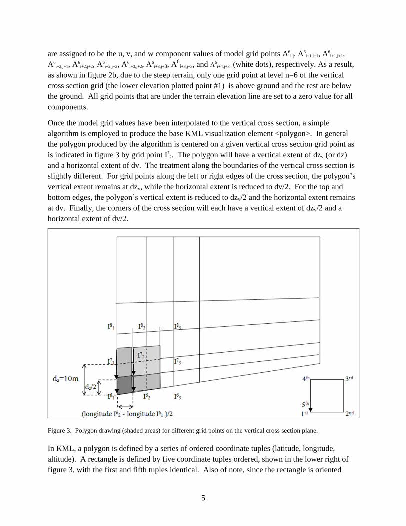
Once the model grid values have been interpolated to the vertical cross section, a simple
algorithm is employed to produce the base KML visualization element <polygon>. In general
the polygon produced by the algorithm is centered on a given vertical cross section grid point as
is indicated in figure 3 by grid point I72. The polygon will have a vertical extent of dzv (or dz)
and a horizontal extent of dv. The treatment along the boundaries of the vertical cross section is
slightly different. For grid points along the left or right edges of the cross section, the polygon’s
vertical extent remains at dzv, while the horizontal extent is reduced to dv/2. For the top and
bottom edges, the polygon’s vertical extent is reduced to dzv/2 and the horizontal extent remains
at dv. Finally, the corners of the cross section will each have a vertical extent of dzv/2 and a
horizontal extent of dv/2.
Figure 3. Polygon drawing (shaded areas) for different grid points on the vertical cross section plane.
In KML, a polygon is defined by a series of ordered coordinate tuples (latitude, longitude,
altitude). A rectangle is defined by five coordinate tuples ordered, shown in the lower right of
figure 3, with the first and fifth tuples identical. Also of note, since the rectangle is oriented
6
vertically, the 1st, 4
th, and 5
th tuples will have the same latitude and longitude, as will the 2
nd and
3rd
tuples. The general formulas for tuples at each vertex of the rectangle are then defined (table
1).
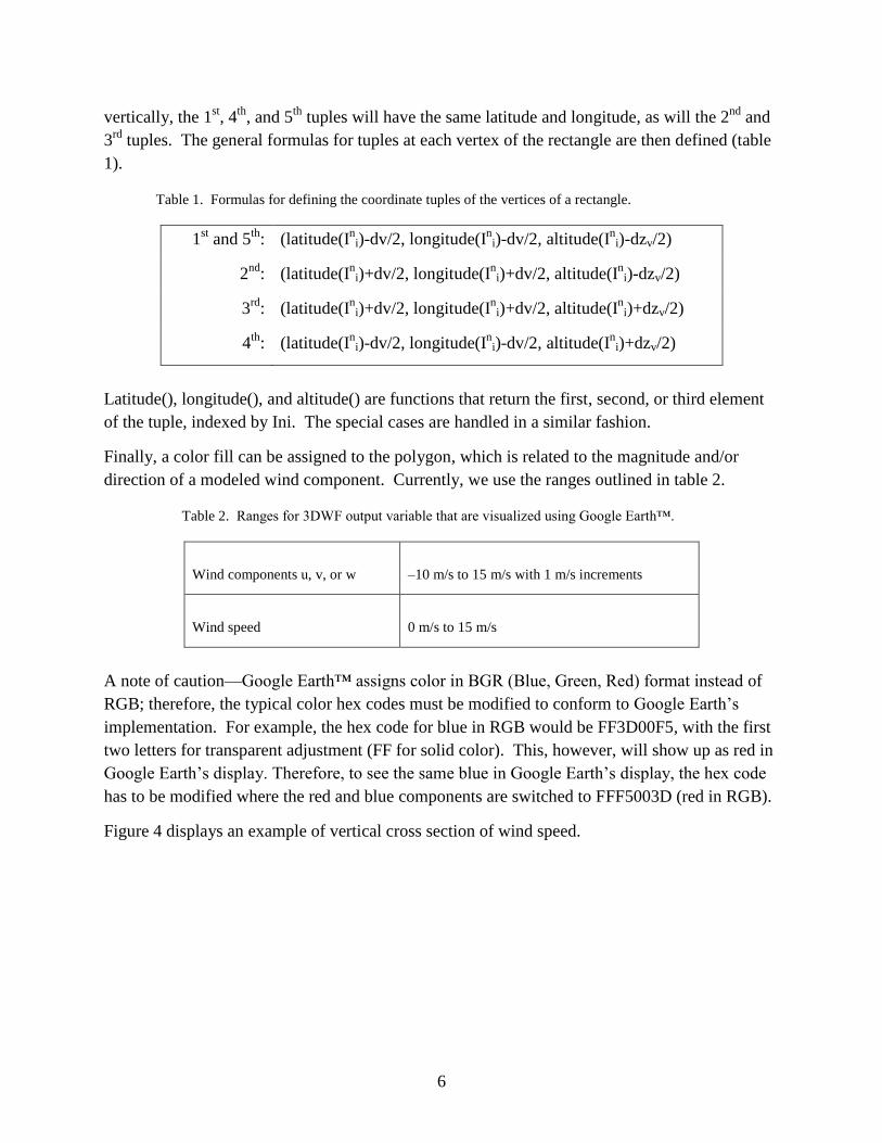
Table 1. Formulas for defining the coordinate tuples of the vertices of a rectangle.
1st and 5
th: (latitude(I
ni)-dv/2, longitude(I
ni)-dv/2, altitude(I
ni)-dzv/2)
2nd
: (latitude(In
i)+dv/2, longitude(In
i)+dv/2, altitude(In
i)-dzv/2)
3rd
: (latitude(In
i)+dv/2, longitude(In
i)+dv/2, altitude(In
i)+dzv/2)
4th
: (latitude(In
i)-dv/2, longitude(In
i)-dv/2, altitude(In
i)+dzv/2)
Latitude(), longitude(), and altitude() are functions that return the first, second, or third element
of the tuple, indexed by Ini. The special cases are handled in a similar fashion.
Finally, a color fill can be assigned to the polygon, which is related to the magnitude and/or
direction of a modeled wind component. Currently, we use the ranges outlined in table 2.
Table 2. Ranges for 3DWF output variable that are visualized using Google Earth™.
Wind components u, v, or w –10 m/s to 15 m/s with 1 m/s increments
Wind speed 0 m/s to 15 m/s
A note of caution—Google Earth™ assigns color in BGR (Blue, Green, Red) format instead of
RGB; therefore, the typical color hex codes must be modified to conform to Google Earth’s
implementation. For example, the hex code for blue in RGB would be FF3D00F5, with the first
two letters for transparent adjustment (FF for solid color). This, however, will show up as red in
Google Earth’s display. Therefore, to see the same blue in Google Earth’s display, the hex code
has to be modified where the red and blue components are switched to FFF5003D (red in RGB).
Figure 4 displays an example of vertical cross section of wind speed.

7
Figure 4. Sample output displaying vertical cross section of wind speed in Google Earth.
2.2 Visualization of the Wind Vector Profile
Google Earth can also be a useful tool for displaying wind vector profiles. Its navigation
features allow users to observe model output from many directions. A similar technique to the
one previously described can be used to create and paint polygons that represent a 3D wind
vector profile at a user specified location within the 3DWF model grid domain. A GUI
application was designed to handle user input interactively. This GUI allows the user to use the
mouse to select points of interest on the Earth’s surface within the given model domain to
acquire latitude and longitude information. This information is then used to extract the wind
vectors for these points and process the profiles for display within Google Earth. Each profile
starts from the ground up to the requested height within the vertical limit of the model’s domain,
with a separation dz between levels. The increment dz (in meters) is determined by the 3DWF
output file. The number of wind vectors or levels at each profile is derived from the requested
height and dz. For example, if the given dz is 20 m, and a user requested a height of 80 m above

8
ground level, the result would be a wind vector profile with five levels. The five levels would be
the data levels that match the heights at 0, 20, 40, 60, and 80 m above ground.
First, for each level in the profile, we must define the wind components (u, v, w), wind speed,
and wind direction. As described earlier, profile level u, v, and w component values are assigned
using a nearest neighbor algorithm. Referring to figure 5, the horizontal wind speed, Vh, and
wind direction, θ, can be calculated using the following formulas. Note that the direction is with
respect to true North, (0o=North, 90
o =East, 180
o =South, 270
o =West) and that the wind is
coming from and follows the meteorological convention.
Vh = sqrt(u2 + v
2 );
θ = 270.0o – atan2(v, u) *180
o /π.
For the 3D display of wind vector data, a pyramidal wind flag is used to represent the vector.
The size of the pyramid is proportional to the magnitude of the total wind. The wind direction is
indicated by the direction that the pyramid points to, conforming to meteorological conventions.
We compute the total wind speed (note that the vertical wind component w is included) as:
V = sqrt(u2 + v
2 + w
2).
The vertical angle of the wind vector α (see figure 5) is calculated as
α = atan2(w,Vh).
z
V
w
y (N)
θ α v Vh
(W) x (E)
(S) u
Figure 5. 3D illustration of wind components (u, v, w), wind speed (V), and wind
direction coming from the SW.
The 3D wind vector flag is constructed with a parallelogram as its base and four triangles with a
common vertex at the apex of the pyramid (figure 6). The centroid of the base parallelogram is
placed at the model grid location given by the tuple (latitude, longitude, altitude). We then
locate the apex of the pyramid, head of the vector, using the following formulas:

9
longitudehead = longitudecentroid + U
latitudehead = latitudecentroid +V
altitudehead = altitudecentroid + W
Here U and V are the u and v wind components that have been converted into the longitude-
latitude reference frame and then scaled by a user defined scale factor. W is the converted and
scaled w component of the wind.
Figure 6. (a) Three-dimensional illustration of a wind direction flag and (b) its projection on the horizontal plane.
We next locate the four vertices of the base using the following formulas. Here, d, measured in
meters, is a user-defined distance that controls the size of the base, and S=1/111133 is a
conversion factor to convert the distance d into degrees for display within Google Earth. For the
two vertices that are on the diagonal of the parallelogram that is parallel to the ground surface we
have:
α
α
d

10
longitudeverparallel = longitudecentroid ± d*S*cosθ
latitudeverparallel = latitudecentroid ± d*S*sinθ
altitudeverparallel = altitudecentroid,
where the application of plus or minus is dependent upon the angles and .
As the vertical wind direction moves upward or downward an angle θ, the second pair of vertices
in vertical direction will be tilted off the vertical line in opposite directions. Their coordinates
can be obtained by using the following formulas:
longitudeververtical = longitudecentroid ± d*S*sinα*sinθ
latitudeververtical = latitudecentroid ± d*S*sinα*cosθ
altitudeververtical = altitudecentroid ± d*cosα
Once the vertices for the vector flag have been defined, there are six total triangles; two define
the base of the pyramid and four define the facets of the pyramid, which can be encoded into the
KML, which is used for display within Google Earth.
Generally, when plotting the wind vector profiles, we need to map the lowest vector to the
appropriate model level. As indicated earlier, we use a nearest neighbor technique for defining
the wind components in the horizontal direction. For the vertical level assignment of the lowest
level, we compute or find the lowest level of valid wind data (i.e., the first model level above
ground). This model level will be the first level defined within the profile to be displayed. We
then extract the remaining requested levels for the profile. Figure 7 illustrates this. In this figure,
assume that dz is defined as 10 m and the user entered a height = 20 m. Therefore, there are three
profile levels requested—one at 0 m, one at 10 m, and one at 20 m. However, since the lowest
valid model wind data for the plotted points 1 and 2 happen to be nearer to the data levels 2 and
3, respectively, the three profile levels at point 1 and point 2 will be defined by the model wind
data from levels 2, 3, and 4, and levels 3, 4, and 5, respectively. The wind flags will then be
displayed at these levels.

11
Figure 7. Wind profile flag adjustment.
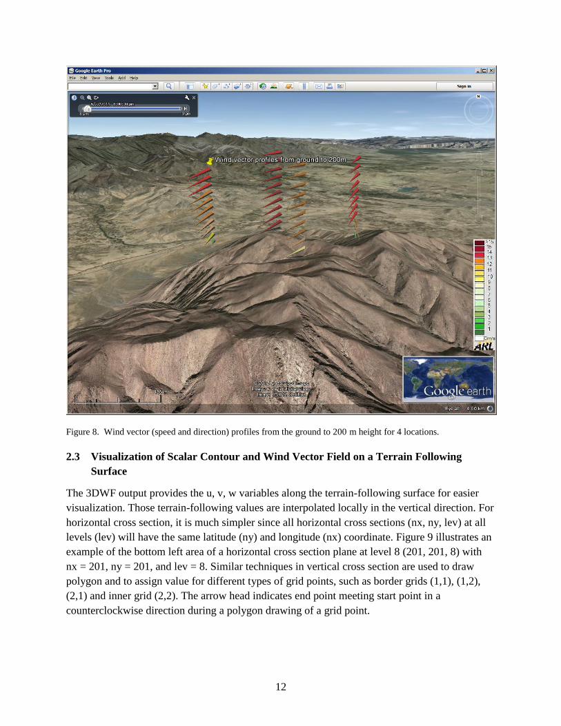
Figure 8 displays a captured simulation of four wind speed and direction profiles between the
ground and a height of 200 m at various locations. The separation between profiled flags
represents dz = 20 m increment. Since Google Earth’s terrain height sometimes does not
perfectly match with the 3DWF’s terrain height, the ground level wind vector flag may disappear
under the Google Earth’s terrain display. In order to avoid this problem, each profile was raised a
short distance above the ground (e.g., 100 m) to ensure the visibility of the wind vector flag at
the ground level. In some cases, a separation of 10 m or 20 m between vector flags can appear
very small in a zoom-out display covering all plotting points, with significant distances between
them. As a result, the vector flags will appear clumped together. For display purposes, the
separation dz between levels was also rescaled and extended, to 5 dz for example, to avoid
crowded appearance. The wind flag’s size is also adjusted to enhance its visualization, as already
mentioned. Notice that the wind speed magnitudes not only are presented by the flag’s lengths
but also by the color scales. The flag’s color helps to identify the wind speed’s range at such
level in the case when the Google Earth’s rotated navigator gives a wrong perspective of the
flag’s actual length. This happens since all flags do not line up in the same wind direction, and as
a result, a view at a particular angle can distort the flag’s actual length. Therefore, the flag’s
displayed lengths should not be used alone to compare the wind speeds between neighbored
wind speed ranges.
12
Figure 8. Wind vector (speed and direction) profiles from the ground to 200 m height for 4 locations.
2.3 Visualization of Scalar Contour and Wind Vector Field on a Terrain Following
Surface
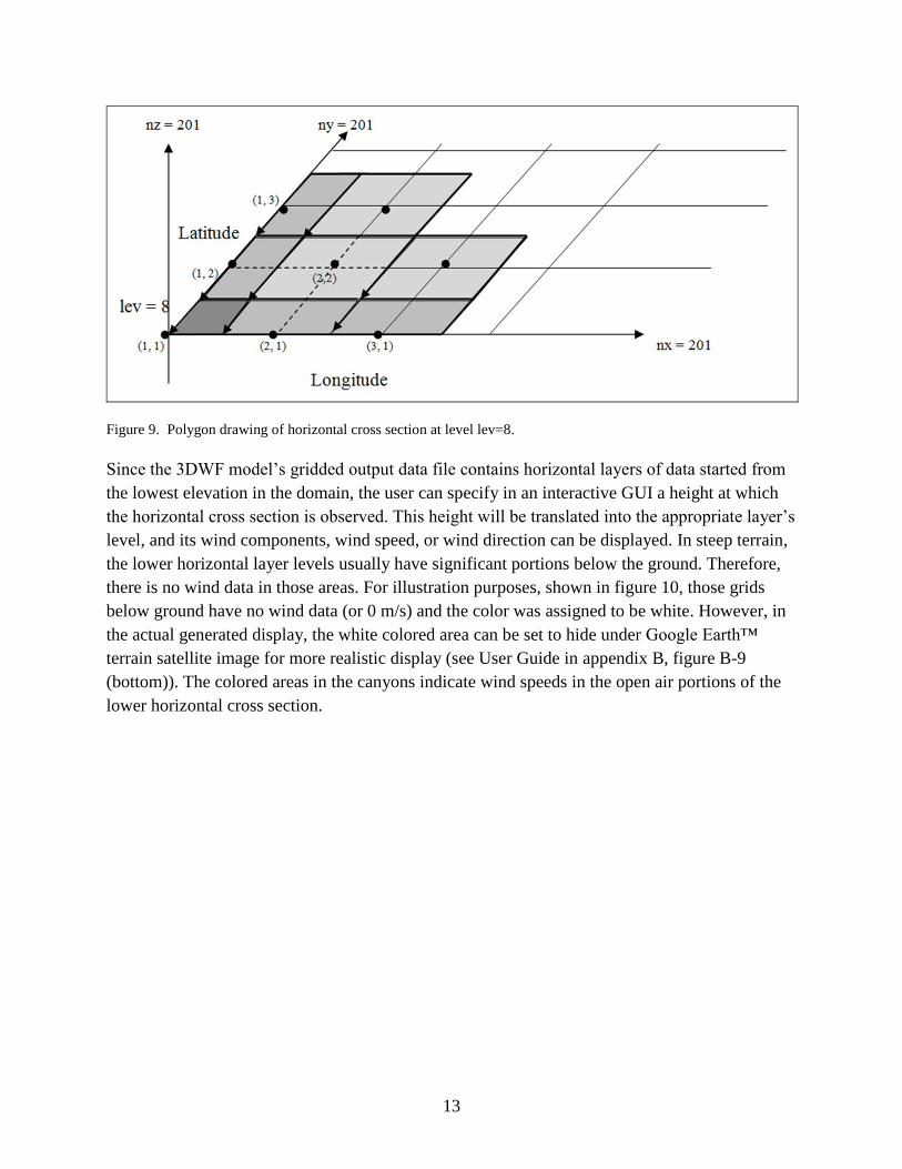
The 3DWF output provides the u, v, w variables along the terrain-following surface for easier
visualization. Those terrain-following values are interpolated locally in the vertical direction. For
horizontal cross section, it is much simpler since all horizontal cross sections (nx, ny, lev) at all
levels (lev) will have the same latitude (ny) and longitude (nx) coordinate. Figure 9 illustrates an
example of the bottom left area of a horizontal cross section plane at level 8 (201, 201, 8) with
nx = 201, ny = 201, and lev = 8. Similar techniques in vertical cross section are used to draw
polygon and to assign value for different types of grid points, such as border grids (1,1), (1,2),
(2,1) and inner grid (2,2). The arrow head indicates end point meeting start point in a
counterclockwise direction during a polygon drawing of a grid point.
13
Figure 9. Polygon drawing of horizontal cross section at level lev=8.
Since the 3DWF model’s gridded output data file contains horizontal layers of data started from
the lowest elevation in the domain, the user can specify in an interactive GUI a height at which
the horizontal cross section is observed. This height will be translated into the appropriate layer’s
level, and its wind components, wind speed, or wind direction can be displayed. In steep terrain,
the lower horizontal layer levels usually have significant portions below the ground. Therefore,
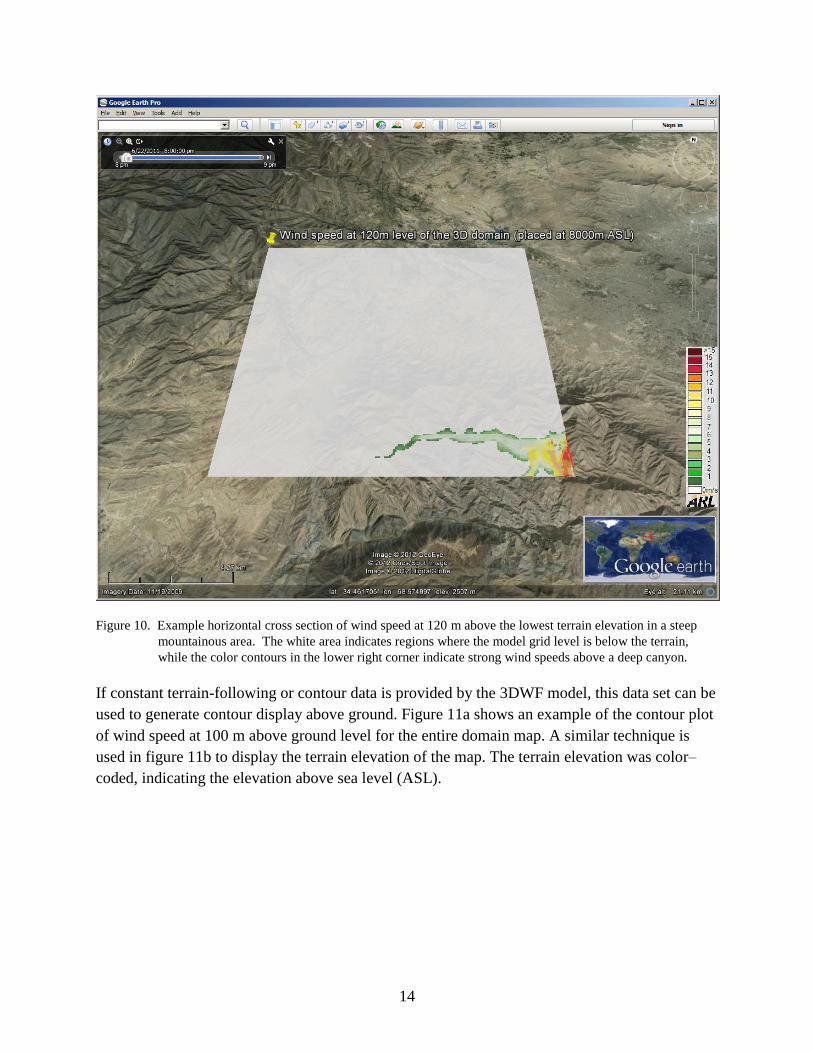
there is no wind data in those areas. For illustration purposes, shown in figure 10, those grids
below ground have no wind data (or 0 m/s) and the color was assigned to be white. However, in
the actual generated display, the white colored area can be set to hide under Google Earth™
terrain satellite image for more realistic display (see User Guide in appendix B, figure B-9
(bottom)). The colored areas in the canyons indicate wind speeds in the open air portions of the
lower horizontal cross section.
14
Figure 10. Example horizontal cross section of wind speed at 120 m above the lowest terrain elevation in a steep
mountainous area. The white area indicates regions where the model grid level is below the terrain,
while the color contours in the lower right corner indicate strong wind speeds above a deep canyon.
If constant terrain-following or contour data is provided by the 3DWF model, this data set can be
used to generate contour display above ground. Figure 11a shows an example of the contour plot
of wind speed at 100 m above ground level for the entire domain map. A similar technique is
used in figure 11b to display the terrain elevation of the map. The terrain elevation was color–
coded, indicating the elevation above sea level (ASL).

15
(a)
(b)
Figure 11. Contour plots on a terrain following surface of (a) wind speed at 100 m above
ground level and (b) terrain elevation.

16
For horizontal cross section of wind direction, a combination of techniques in constructing the
3D wind direction flag and in horizontal cross section display of wind speed described
previously is used to create a horizontal plane of wind direction flags. Figure 12 shows an
example of wind direction vectors at 100 m above ground observing from the south. As
mentioned in the wind direction profile section, wind speeds also are indicated by the flag’s
length and by the color scale.
Figure 12. Wind vector field plotted on a terrain following surface 100 m above ground level. Every 2nd
vector has
been plotted.
From this display, the user is able to observe both wind speed and direction of the vector flow
field realistically in a 3 dimensional visualization. Moreover, Google Earth provides convenient
capabilities, such as navigating in different directions, adjusting for the time of day’s brightness,
observing wind features on top of the real terrain satellite image below, or creating a fly-thru or
around animations for demonstration purpose.
17
3. Graphical User Interface (GUI)
The GUI is comprised of three modules or menus, each designed to handle a different task. The
three tasks are to (1) define a vertical cross section, (2) define a horizontal cross section, and (3)
define wind direction profiles. The three modules are linked together in order to facilitate the
user’s navigation from one module to another directly. Each module requires a few simple
interactive inputs prior to processing the data through built-in Fortran90 executable code. This
section discusses the implementation of these GUI modules and the interfaced Fortran90
programs.
3.1 GUI Module Implementation
JavaScript provides a simple yet powerful means to develop GUIs for Web-based applications. A
number of toolkits exist that provide for a simple foundation to build rich user interfaces. One
such toolkit for geographic information is provided by Google through the Google Earth API.
By design, JavaScript limits access to local resources. This is done to protect against the
execution of malicious code. However, ActiveX components or XPCOM extensions can be used
by JavaScript to write data to the local file system. Since there is an inherent risk, it is very
important to only use these types of objects (ActiveX or XPCOM) from a trusted source in order
to minimize the exposure of a computer system to malware. Without the availability of these
trusted components, the use of JavaScript for the implementation of a GUI for the tool would be
less than ideal.
While hypertext markup language (HTML) is an open standard, its implementation by the
various vendors is often muddled with proprietary extensions. Though we have tried to maintain
compatibility with the various Web browsers on the market today, the requirement to write files
on the client side limited our initial implementation to Microsoft’s Internet Explorer (IE) Web
browser. The Web application renders fine in Mozilla Firefox and is fully functional, sans the
capability to save the geographic data through the GUI. Currently, a PC Vista user who prefers to
run on Mozilla Firefox can also save data to a local file by downloading an add-on named IE
Tab2 (FF3.6+), which is freely available on the Internet. This add-on allows switching to IE from
inside Firefox in order to run the GUI. The procedure to obtain the add-on is provided in
appendix A.
The GUI modules were designed based on the most recent version of the Google Earth API
6.0.0.1735 (beta), rendered in Mozilla Firefox (see User Guide in appendix B). The GUI has
been implemented as a Web page using HTML and JavaScript. The initial interface discussed
here was to demonstrate a proof of concept and the capability to leverage the Geographic
Information System (GIS) information available through the Google Earth API. The interface
provides the user an interactive way to display scalar variables, such as contours of wind speed at
18
different layers above ground using horizontal cross sections and vertical cross sections, as well
as wind direction profiles at user defined locations. The GUI basically consists of two parts—a
GIS map panel on top, which automatically detects and zooms in to the location provided in the
3DWF parameter file, and a menu of buttons and some simple interactive input boxes at the
bottom. The GIS map panel is an embedded Google Earth display, with a simple navigator
control to enable viewing the 3D display in all directions.
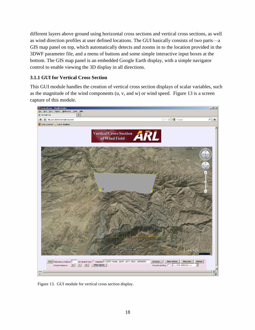
3.1.1 GUI for Vertical Cross Section
This GUI module handles the creation of vertical cross section displays of scalar variables, such
as the magnitude of the wind components (u, v, and w) or wind speed. Figure 13 is a screen
capture of this module.
Figure 13. GUI module for vertical cross section display.

19
The first button from the left is the “Help” button to guide the user with the procedure for
creating a vertical cross section and helpful hints. In this module, the user selects two locations
on the map to define the vertical cross section plane. These two coordinate pairs of longitude
and latitude are then saved in a text file, named as Lineendscoords.txt. This file will be read and
the coordinates processed by the built-in Fortran90 code upon one of the display buttons being
clicked by the user. The display buttons consist of “Display u”, “Display v”, “Display w”, and
“Wind speed”. The user can choose to click any one of them to see the display in a new Google
Earth KML window (see figure 4 above is the result after “Wind speed” button was clicked).
The Google Earth window is also saved in a KML file, with distinctive filename, in a designated
directory such as C:/3DWF. The User Guide in appendix B will provide more details on how to
operate this module.
3.1.2 GUI for Horizontal Cross Section
This GUI module handles the creation of horizontal cross section displays of scalar variables,
such as the magnitude of the wind components (u, v, and w) and wind speed, as well as the
vector wind display. Figure 14 is a screen capture of this module.

20
Figure 14. GUI module for horizontal cross section display.
For this module, there is no mouse plotting involved since the horizontal display will cover the
entire given domain. However, there are still a few required interactive inputs that are saved in a
text file named “Inputinfor.txt”. This file will be read by the built-in executable Fortran90 code.
The first text input box from the left is for the user to define the level of the model output to be
displayed. The value entered is required to be an integer multiple of dz. Note that this height is
given in meters above the lowest terrain elevation point (level number 1) within the given map.
The entered height will result in display of a horizontal layer at the defined height. Once the text
input boxes have been entered, the user can then select one of the seven plot buttons. The seven
buttons are labeled, “u”, “v”, ”w”, “Speed”, “Horiz vectors”, “Domain vectors”, and “Terrain
elev”. When clicked they produce the contours for the wind components, wind speed at the user
defined height, and the terrain elevation contours, respectively. The two vector display buttons,

21
“Horiz vectors” and “Domain vectors”, produce slightly different results. As indicated by its
label, the “Horiz vector” button will produce a wind vector plot at the user-defined elevation.
The “Domain vector” button will produce a multi-layer wind vector plot of all the model levels
up to the height requested by the user. The user is cautioned, however, that this option will result
in the generation of a very large KML file if the default flag density is used. It is also
noteworthy to point out that the computation and render time significantly increase and can
produce a much more cluttered display.
For this report, the maximum entered height is 200 dz, representing the highest level number nz
= 201. For example, if dz = 20 m, then the maximum allowed height to be entered is 200 x 20 =
4000 m for level 201. Figure 10 illustrates a display (KML file) of wind speed at 120 m or level
7 with dz = 20 m. The white area indicates no wind data (or 0 m/s), as this lower horizontal
layer cuts through the steep mountains. Only those areas above the terrain have wind speed data
(shown in colored areas).
For the case of contours of a scalar on a terrain-following surface, if the user enters a height that
matches the height of a precomputed surface within the model output, then the GUI will give the
user two options whether to display this terrain-following surface or the model’s level data. An
example is shown in figure 11a. If the entered height doesn’t match any, then the level data is
displayed.
The wind flag’s size and flag density text input boxes (each defaults to 1) allow the user to
manipulate the wind direction flags for better visualization. Notice that these two input boxes
are applied only for the two wind vector buttons, “Horiz vectors” and “Domain vectors”. The
higher the integer number entered in “Wind flag’s size” input box, the bigger the flag will
appear. The integer number entered in “Flag density” input box is actually the number of grid
point to be skipped in between flags. Therefore, a 1 means full density for the wind vector plot
on the map. An input of 2 would indicate half density with every other vector not being plotted.
The rendering speed of the display is heavily dependent upon the flag density and size. For
quicker display rendering, it is recommended to increase the flag size and flag density so as to
avoid a crowded appearance. The “Terrain elev” button is used to generate a contour display of
the model terrain elevation above sea level.
3.1.3 GUI for Wind Direction Profiles at User Defined Locations
This GUI module, as shown in figure 15, allows the user to generate and display wind direction
and wind speed profiles at user defined locations within the modeled domain. An example is
displayed in figure 8. The user defines the locations to be plotted by clicking the mouse within
the model domain. The coordinate pairs of latitude and longitude are recorded, and saved in a
file called “Plotscoords.txt” (see appendix B). Currently, for practical purpose, the number of
profiles is limited to 50. This GUI requires a few simple interactive inputs. The “Total Frames”
input box (default is 1) is the number of frames to be generated in a time sequence. Each frame
is a display of the user selected profiles. In the “Height” text box, the user defines the height (in

22
m) at which the user would like to observe all the wind direction profiles (in dz increment) down
to the ground. The “Wind flag’s size” is an integer factor used to increase or to reduce the flag’s
size. These inputs are saved in a file named “Profile.txt”.
Figure 15. GUI module for displaying wind vector profiles at 5 user defined locations.
3.2 Fortran90 Programs
Since execution speed was a significant factor in the development of our application, the
algorithm(s) have been implemented using Fortran90. Each GUI module directly interfaces with
each Fortran90 program written to perform the respective algorithm described in the previous
sections. Basically, each program reads in and processes the 3DWF output files such as
“Kabul_3DWF_2011_0623_120000000.gdat” and “3DWF_parameter.txt”. The 3DWF model
output files contain gridded latitude and longitude wind components and terrain elevation, as
23
well as the model map domain information, such as size and location, represented by the center
of the model given in latitude and longitude. Any interactive actions with the GUI modules—
e.g., user’s inputs and map plotting—also are read by the programs prior to the processing and
generation of a series of text files, which are necessary for the creation of polygons of the KML
display.
For the vertical cross section, the Fortran90 code generates the files Gridsinfor.txt,
Polycellucoords.txt, Polycellvcoords.txt, Polycellwcoords.txt, and Polycellspcoords.txt to
prepare necessary inputs for the JavaScript code in the GUI, and subsequently to create the
Google Earth KML file for the cross section display.
For the horizontal cross section, the Fortran90 code generates the following files:
GridsinforH.txt, Polycelluhoriz.txt, Polycellvhoriz.txt, Polycellwhoriz.txt, Polycellsphoriz.txt,
Plothorizonwinvec.txt, Plotvolumewinvec.txt, and Polycellterhoriz.txt. The file GridsinforH.txt
contains the model grid information. The files with the prefix “Polycell” contain sequential data,
for points 1 through 5, defining a rectangle of grids/cells or polygons in order for the JavaScript
code to place them correctly in a KML file. The files Plothorizonwindir.txt and
Plotvolumewinvec.txt contain sequential data, for points 1 through 4, which are used to define
the 6 triangles that comprise the pyramidal wind flags.
For the wind direction profiles defined at user specified locations, the Fortran90 code produces
only one file named “Plotwindir.txt”, which is necessary for the creation of the vertical 3D
pyramid wind direction flags in a KML file.
4. Conclusion
As mentioned in the introduction of this report, there is a need for the development of advanced
techniques to assist scientists and researchers in observing visually the modeled wind’s behavior.
This is especially important to the Army in investigating and predicting wind flows in urban or
mountain areas. In supporting the improvement of the 3DWF model, three visualization
techniques used in the visualization of geosciences data on Google Earth have been adopted and
implemented. The results have proven not only to be more realistic and professional in
appearance, but also provide a convenient method for the quick observation and navigation of
the 3DWF modeled wind field in all directions.
Currently, we have developed three new features, a method to create and display the vertical
cross section of wind field, a method to create and display the horizontal cross section of wind
field, and a method for the creation and display of the wind direction and wind speed profiles.
The vertical cross section helps the user to observe the wind speed’s distribution vertically via
contours. The result not only provides an indication of modeled wind speed differences at
different altitudes, but it also reveals possible effects of the terrain at the lower boundary. The

24
horizontal cross section assists in the visualization of terrain elevation, horizontal layers of wind
components, wind speed, and wind direction, as well as their contour above ground level when
data is available.
As described in displaying wind speed and wind direction profiles above ground section, the
smaller the increment dz is used to generate data levels, the more accurate the adjustment to the
correct profiles’ heights. The other option to obtain correct profiles without this adjustment is to
produce contour data layers closer to the ground.
Based on this work, other applications can be adapted to observe other types of scalar data in
complex areas, such as plume concentrations in a complex terrain. Future development is
planned to include the display of isosurfaces.
25
5. References
Google API Web site. http://code.google.com/apis/Earth/ (accessed July 2011).
Huynh, G.; Wang, Y.; Williamson, C. Building and Vegetation Rasterization for the Three-
dimensional Wind Field (3DWF) Model. U.S. Army Research Laboratory Publication 2010,
1-19.
Wang, Y.; Williamson, C.; Garvey, D.; Chang, S.; Cogan, J. Application of a Multigrid Method
to a Mass Consistent Diagnostic Wind Model. J. Appl. Meteorol. 2005, 44, 1078–1089.
Wang, Y.; Williamson, C.; Huynh, G.; Emmitt, D., Greco, S. 2010, Diagnostic Wind Model
Initialization over a Complex Terrain Using the Airborne Doppler Wind Lidar Data. Open
Remote Sensing Journal 2010, 3, 17–27.
Yamagishi, Y.; Yanaka, H.; Suzuki, K.; Tsuboi, S.; Isse, T.; Obayashi, M.; Tamura, H.; Nagao,
H. Visualization of Geoscience Data on Google Earth: Development of a Data Coverter
System for Seismic Tomographic Models. Computers & Geosciences Journal 36 2010, 373-
382.

26
INTENTIONALLY LEFT BLANK.

27
Appendix A. Procedure to Download Add-on IE Tab2 for Firefox 3.6+ (or any
later version)
Activate Mozilla Firefox (or Internet Explorer, if using computer with Windows operation other
than Vista). For Vista users, an add-on named IE Tab2 (FF3.6+) freely available from the
Internet must be installed. Follow steps a to g to download.
a. Open Firefox Web page by clicking “Getting Started”.
b. Move cursor to “Add-ons” option from the top of the page and select “Desktop Add-ons”.
c. A “Firefox Add-ons” window will appear. Type “IE” inside the slot “search for add-ons”
and click the green arrow at the end to start searching.
d. A list of all current available add-ons developed by the Firefox community will
appear and be ready for download. Select the add-on named “IE Tab 2 (FF 3.6+)” or
similar latest Add-ons and click on the green button “Add to Firefox” to add.
e. A small window will appear with a warning message and with the address link to the add-
on. Click on the address link to activate the “Install Now” button.
f. Click on the “Install Now” button to start installation. A new small window will
appear, and when the installation is done, click on “Restart Firefox” button to activate the
new feature. Notice a small Firefox logo will appear at the bottom right corner next to the
key lock logo.
g. Clicking on that Firefox logo will switch to an IE logo. It will then enable the user to work
inside IE environment and allow saving data file to the local disk. To switch back to
Firefox, click on the IE logo to change.

28
INTENTIONALLY LEFT BLANK.
29
Appendix B. User Guide for the Wind Field Visualization GUI
This user guide is intended to help a new user to operate the Wind Field Visualization Graphic
User Interface (GUI). Currently, the GUI works on PC and requires basic access to Google
Earth, Mozilla Firefox, and Internet Explorer browsers. The GUI software package includes
following files:
MainMenu.html
VerticalCross.html
HorizontalCross.html
WinvecProfiles.html
(Isosurface.html is under development)
Verticalcross.exe
Horizontalcross.exe
Winvecprofiles.exe
(Isosurface.exe is under development)
ARLlogoMain.png
ARLlogoVer.png
ARLlogoHor.png
ARLlogoPro.png
(ARLlogoIso.png is under development)
Wspdspec.jpeg
Wspdonlyspec.jpeg
Terelevspec.jpeg
WV.shortcut (for MainMenu.html)
WVUserGuide.doc
All program files and generated files (in bold letters) should be stored in the same subdirectory,
preferably C:/3DWF/. Currently, there are four separate modules or windows to generate and
control the displays of three different aspects: vertical cross section, horizontal cross section, and
wind vector profiles at plotted locations (isosurface option is under development). Their
JavaScript filenames are VerticalCross.html, HorizontalCross.html, and
WinvecProfiles.html. Each file interfaces with a separate Fortran90 executable file having
similar name such as Verticalcross.exe, Horizontalcross.exe, and Winvecprofiles.exe. These
Fortran90 files, which were written using Microsoft Visual Studio 2010, help to prepare
polygons’ coordinates necessary for the graphic rendering in Google Earth. Other image files in
png and jpeg formats are for the GUI’s titles and color scales. The software package starts with a
short cut logo “WV” created for the file MainMenu.html.

30
B-1 Main Menu
To start the operation, double-click on the WV logo or the MainMenu.html file in the
subdirectory. The main window will open, as seen in figure B-1.
Figure B-1. The main menu for the Wind Field Visualization application.
There is a drop-down menu named “Link selection” at the bottom of the page to allow the user to
select any of the three mentioned features.
B-2 Vertical Cross Section
The first feature on the list is “Vertical Cross Section”. A click on this option will prompt a new
window for VerticalCross.html file, as shown in figure B-2.

31
Figure B-2. GUI window for vertical cross section.
In order for the program to gain access to the stored executable and data files, and also to save
generated files, the GUI must operate in an IE environment and in which Active X control must
be allowed. Click on the Firefox logo at the lower right corner of the page to toggle it to IE
operation. A warning message will pop up about activating Active X control. Click “Yes” to
accept. In the case when a 3DWF_parameter.txt file is given, the software will automatically
detect the latitude and longitude coordinates of the center of the data domain and zoom in at such
location. Figure B-2 is an example of this zoom-in.
1. For each module, always click on the “Help” button at the lower left corner first to review
instructions and explanations.
2. The vertical cross section GUI allows either to generate display for one single vertical cross
section (single frame of display) or to generate display containing multiple vertical cross

32
sections (multiple frames). For multiple vertical cross sections, if they are all at the same
time (same data file), the multiple frames display will appear as though they are in one
image. This feature allows the user to observe the vertical changes at different locations
within the domain map. For multiple vertical cross sections at the different times (different
data files), it will allow the user to view each vertical cross section (or frame) at a time by
sliding the Google Earth’s time scale located at the top left of the display. It is extremely
difficult if not impossible for a user to re-plot at an exact location. Therefore, in the case
when the user would like to observe the changes at an exact location but at different
dates/times, this module will also allow retention of the previous plotted cross line for the
next frame (different date/data file).
For single frame or vertical cross section, enter 1 (default) into the slot “Total cross
sections”.
For multiple frames of multiple vertical cross sections, enter the total number into the slot
“Total cross sections”. This number will automatically count down as the program finishes
processing each frame.
3. The check box “Combined View” allows the user to combine all vertical cross sections
from different frames (different times) to be viewed together in one display, instead of
moving the Google Earth time scale to see each vertical cross section. A check mark on it
will prompt an explanation message. Leave it unchecked for a single frame.
4. In the next long slot, the GUI allows the user the ability to browse the local directory in
order to select an input data file for a frame. Click on the “Browse” button to select an
interested file. Double click on the file or move the cursor to the file, highlight, and click
“Open”. The file will show up inside the “Data file” slot.
5. Since vertical cross section requires two plotted points inside the domain’s horizontal map,
outline of the map’s boundary must be drawn to prevent plotting outside of the intended
area. Plotting can only be allowed after this outline is drawn. Click on “Map outline”
button to display the yellow outline as shown in figure B-3. “Map infor” button displays
basic parameters of the outlined map such as center coordinates, dx, dy, dz, nx, ny, and nz.
This information is given from the output of the 3DWF model.

33
Figure B-3. Map outline display.
6. Next, move cursor and click left mouse button to plot two points inside the yellow outlined
map for the two endpoints of an intersect line between the vertical cross section plane and
the Earth’s surface (figure B-4). After the second click, a message will inform about which
file (currently named as Lineendscoords.txt) the latitudes and longitudes of the plotted
points have been saved in. Coordinates of each point can be seen by left-clicking the mouse
on its yellow pin. A grey area is drawn to represent the vertical cross section defined by the
two plotted points. This display is solely for marking purpose on the menu’s map and not
an actual generated image.

34
Figure B-4. Two user selected points forming intersect line.
7. There are four different display features for this GUI: u, v, w, and wind speed. Once a wind
display feature button is clicked, it will prompt an OK/Cancel self-explanatory instruction
on proper steps to proceed. In the instruction, there is an option to allow combination of
this vertical cross section and a horizontal cross section (of the same data file) that will be
generated upon finishing with the vertical cross section. Figure B-7 in section 9 will
illustrate further of this option.
If the user intends to do this, then “OK” button must be clicked to proceed.
If the user simply generates a single vertical cross section, then click Cancel.
Selecting OK will result in two generated KML files—one for current vertical cross section
and one to be amended with the horizontal cross section later.

35
After selecting OK or Cancel, the GUI will execute the Fortran90 code
“Verticalcross.exe” in order to prepare an appropriate polygon data file necessary for the
polygon drawing in a Google Earth’s KML file. Depending which feature was selected, the
generated polygon data file will be one of the following four files, for u, v, w, and wind
speed, respectively.
Polycellucoords.txt
Polycellvcoords.txt
Polycellwcoords.txt
Polycellspcoords.txt
These polygon data files with prefix “Polycell” contain the vertical cross section’s grid
point’s longitude, latitude, height (ASL in meter), and the real value of either u, v, w, or
wind speed in meters per second.
68.9260864257812, 34.4337882995605, 2425.096, 8.02551174163818
68.9261968271020, 34.4337908470172, 2425.096, 8.02551174163818
68.9261968271020, 34.4337908470172, 2435.096, 8.02551174163818
68.9260864257812, 34.4337882995605, 2435.096, 8.02551174163818
In addition, a file named Gridsinfor.txt is also generated. It contains information in the
order as shown below. For example, if nx = 201, ny = 201, and nz = 201 of a given
domain, the number of vertical grid points found on the intersection line is 442, the level
number ID of the lower level of the two plotted points is 28, and the minimum height
above sea level (ASL) of the terrain within the domain is 1891.02 m.
201 201 201 442 28 1891.02
A warning message will prompt to advise on what to do while processing and generating of
the mentioned files. If the intersection line is long enough result in a large vertical cross
section, then a black command window will appear during execution of the Fortran90 code.
It is important to let the program finish (after the black window disappears and the
“Polycell…” is completely generated), or a premature click on the “OK” button will mess
up the creation of the display file.
After the GUI is done generating those files, the user can click OK in the warning message
and the GUI will start creating KML file. The KML file will be uniquely named by
combination of the data file’s name, “Ver” for vertical, wind feature, and an endpoint’s
longitude. For example, a file name for a vertical cross section of u wind is:
Kabul_3DWF_2011_0623_120000000Veru68.93826293945312.kml
Upon finishing the creation of KML file, the GUI will also automatically display the vertical
cross section in Google Earth™ as shown in figure B-5.

36
Figure B-5. Example of a vertical cross section displayed in Google Earth.
2. For multiple vertical cross sections (or frames), a message will pop up after each frame is
done to remind the user to select the next data file for the next frame or the next vertical
cross section. The Google Earth™ display will show up only after all frames are processed.
The user can use the mouse cursor to slide the time scale located at the top left of the
Google Earth™ window to observe subsequent frames (figure B-6).
3. Since it is almost impossible to re-plot two points at exactly the same latitude and longitude
on map, the GUI can allow option to reuse the original two plotted points in the case when
the user would like to generate the subsequent vertical cross section at exact the same
location. Subsequent self-explanatory messages will appear to allow this flexibility. The
multiple frames feature allows the user the ability to observe the changes at different
locations of vertical cross sections (same time of different times), or the changes at the
same location but at different times/dates.
For a very large vertical cross section, IE will run slowly and prompt a warning message
with the headline “Stop running this script?” from time to time. This is normal and the user

37
must click on “No” to continue. This message may repeat several times until a “Done”
message appears. Click OK to start the display in Google Earth™.
Figure B-6. Multiple vertical cross sections displaying wind speed at 2 different locations (top row) and at 2
different times for the same location (bottom row).
4. Combination multiple cross sections in one single image: As mentioned previously, this
convenient feature allows the user to observe different aspects (vertical and horizontal) or
at different locations (of the same aspect) in one single image. Figure B-7 top left displays
two different vertical cross sections at different times/dates (sliding time scale), and top
right shows two different vertical cross sections at the same time (same data file).

38
Figure B-7. Example of multiple cross sections displayed in one Google Earth frame. Top left displays two
vertical cross sections at different locations and times. Top right displays different locations at the
same time. Bottom displays a combination of a vertical cross section and a terrain following surface
(horizontal cross section) at the same time.
5. For a combination of vertical and horizontal cross sections, the display in figure B-7
bottom row will only show up after the user has generated the horizontal cross section part
in the next horizontal cross section module.
6. Other useful buttons/features:
Reload button allows refreshing the menu before starting a new session.

39
Checkmark slot ‘Disable plotting’ disables plotting all together. This feature helps the user
to pan the map by using mouse’s cursor without plotting latitude/longitude point. The user
also can avoid plotting while panning by simply use the Google Earth’s pan navigator
located at the top right side. To enable plotting again, click the slot to remove the
checkmark.
The Link selection at the bottom right is enabling the user to go directly back and forth
between modules.
B-3 Horizontal Cross Section
1. For Horizontal Cross Section as shown in figure B-8, click “Help” button to review
instructions and explanations.
Figure B-8. Horizontal Cross Section GUI.

40
For this module, there is no mouse plotting needed since it will display the entire horizontal
map. Therefore, there is no need to use “Map outline” button. The top row’s slots and
buttons have already been explained previously. This GUI will detect the dz vertical
increment value given by the 3DWF’s parameter output file in order to alert the user to
enter a correct height in the “Height (m)” slot.
Enter or change the values in the first three slots of the second row:
2. Height: Since horizontal levels are separated by an increment dz, the entered height of a
level must be a multiple value of dz.
3. Vector’s size: This slot is applied only for “Horiz vectors” and “Domain vectors” feature
buttons. Default value is 1.0. A number greater than 1.0 will increase the size of the wind
vector flag. This option helps to enhance visibility of the wind vector flags in the case
when the map is zoomed out far enough to cover the entire domain.
4. Density factor: This slot is applied only for “Horiz vectors” and “Domain vectors” feature
buttons. The default factor for “Density factor” slot is 1 for plotting wind vector flag at
every grid point on the horizontal domain. A value of 2 means skipping one grid point
before plotting the next wind vector flag, or reducing the number of flags by half. A value
of 3 means skipping every 2 grid points, and as a result, reducing the number of wind flags
to one-third, and so on.
5. After all inputs are entered correctly, click one of the wind feature buttons (u, v, w, Speed,
Horiz vectors, and Domain vectors) or “Terrain elev” to process the display.
As mentioned in the vertical cross section, first, an alert message will ask whether the user
would like to combine this horizontal cross section with the vertical cross section, which
has just been generated from the previous module for the same time/date case only.
Clicking OK will cause the GUI to generate two KML files, one for single horizontal cross
section display and one to display the combination after this horizontal portion is amended
to the vertical portion of the previously saved KML file (as explained in Vertical Cross
Section module).
Click Cancel for generating a single horizontal cross section only.
If generating multiple horizontal cross sections or frames, then this message will show up
during the last frame and the user can click Cancel to process the last frame.
For this module, the Fortran90 code will generate following polygon data files:
Polycelluhoriz.txt, Polycellvhoriz.txt, Polycellwhoriz.txt, Polycellsphoriz.txt,
Plothorizonwinvec.txt, Plotvolumewinvec.txt, and Polycellterhoriz.txt

41
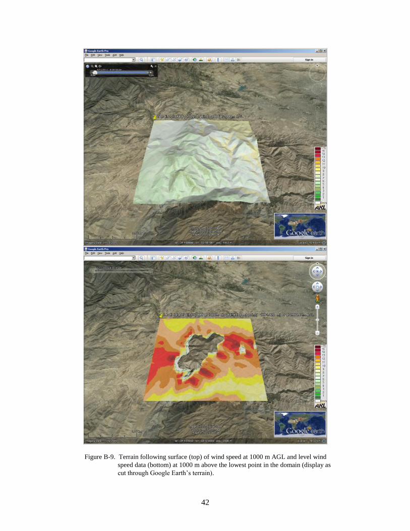
6. For contour display, currently the 3DWF model produces contour data at 20, 100, 200, 300,
400, 500, 600, 700, 800, 900, and 1000 m above ground level (AGL), and this GUI has
been customized to accommodate contours at these specific heights only. If contour data is
also available at an entered height, then the GUI will detect and give the user two options
on whether to generate the contour display or to generate the horizontal level data display.
If an entered height doesn’t match with one of the available contour data levels, then the
GUI will plot just the horizontal level data. Figure B-9 captures an example of contour
display (top) at 1000 m AGL and of level data display (bottom) at 1000 m above lowest
point in the domain.
42
Figure B-9. Terrain following surface (top) of wind speed at 1000 m AGL and level wind
speed data (bottom) at 1000 m above the lowest point in the domain (display as
cut through Google Earth’s terrain).
43
7. Horiz vectors: This feature will plot 3D wind vector flags on a horizontal plane, either as
terrain followed contour plane above ground level if the contour data is available (figure
12), or as a flat horizontal level if contour data is not available.
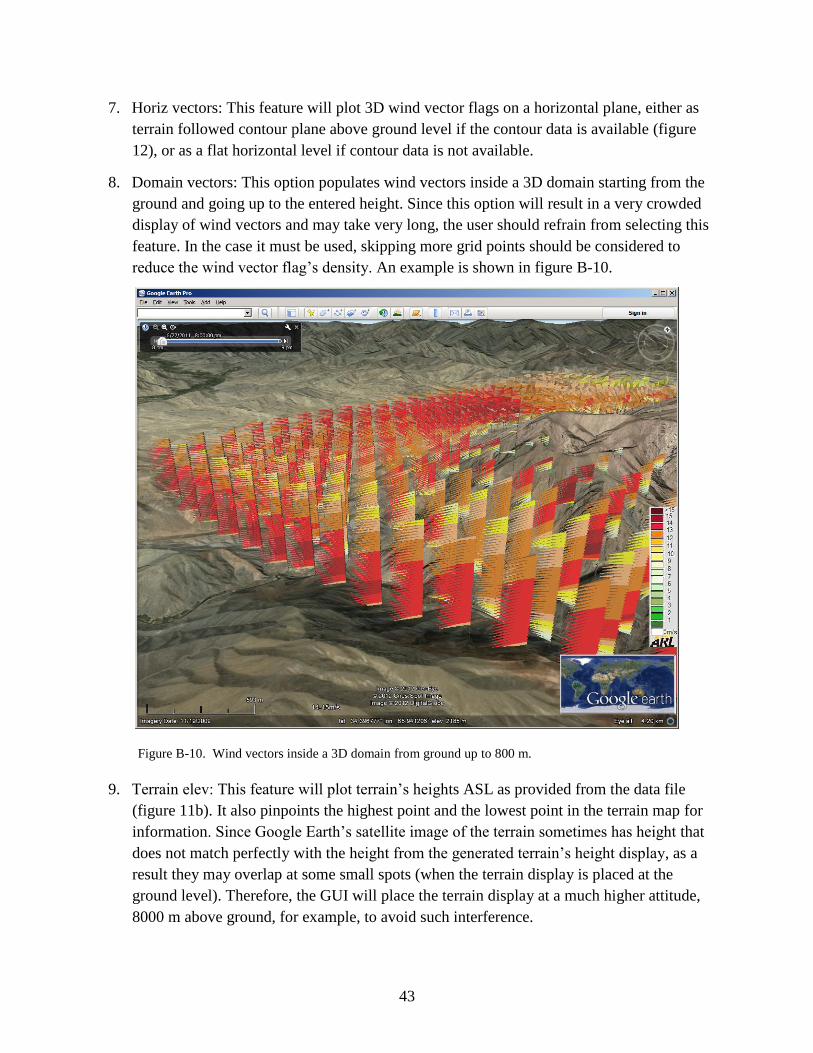
8. Domain vectors: This option populates wind vectors inside a 3D domain starting from the
ground and going up to the entered height. Since this option will result in a very crowded
display of wind vectors and may take very long, the user should refrain from selecting this
feature. In the case it must be used, skipping more grid points should be considered to
reduce the wind vector flag’s density. An example is shown in figure B-10.
Figure B-10. Wind vectors inside a 3D domain from ground up to 800 m.
9. Terrain elev: This feature will plot terrain’s heights ASL as provided from the data file
(figure 11b). It also pinpoints the highest point and the lowest point in the terrain map for
information. Since Google Earth’s satellite image of the terrain sometimes has height that
does not match perfectly with the height from the generated terrain’s height display, as a
result they may overlap at some small spots (when the terrain display is placed at the
ground level). Therefore, the GUI will place the terrain display at a much higher attitude,
8000 m above ground, for example, to avoid such interference.

44
10. Interactive inputs will be saved in a file named “Inputinfor.txt”. The content of this file is
listed as following.
4000
1.0
4
0
0
Kabul_3DWF_2011_0623_120000000
4
1
The first row is the entered height in meters.
The second row with default value of 1.0 is the wind vector flag’s size.
The third row is the density factor. 4 means skipping every 3 grid points before displaying
the vector at the fourth grid point. For this example, the number of vector flags will be
reduced to one-fourth of the original number (at every grid point).
The fourth row with 0 means generating for a single frame or cross section, and 1 signal
generating multiple frames or multiple cross sections.
The fifth row with 0 means to process data and 1 means to draw map’s outline only.
The sixth row is the data file’s name.
The seventh row is the ID number for one of the display feature buttons (4 is for “Wind
speed” button).
The last row will have values of 1 and 0. One or zero is translated from the user’s respond
to the question whether to choose between generating contour (click OK) or level data
(click Cancel) display, respectively.
For this module, the process might take longer for wind vector display depending on the
size of the domain map and the number of generated flags. Therefore, the user may have to
wait a little longer.
This module will generate an information file named as GridsinforH.txt, which contains
information of the number of grid points on x, y, z coordinate, the number of plotted wind
vector flags along the x or y coordinates, and the minimum and maximum height (ASL and
in meters) of the map’s terrain. For the following example, if the number in “Density
factor” slot is 3, then the program will skip every 2 grid points and plot at the third grid
point. Therefore, it will plot a total of 67 wind vector flags on x and y coordinates. The
lowest point and the highest point of the terrain within the map are 1891.02 m and
3193.579 m, respectively.

45
201 201 201 67 1891.020 3193.579
Other generated text files are for the rendering of the polygons in Google Earth™ displays,
as mentioned previously. However, for wind vector display, the polygon coordinates file
Plothorizonwinvec.txt contains additional data columns necessary for the rendering of 3D
wind vector flags. The third column is the height of each corner of a triangle polygon of a
3D wind vector flag. The fourth column is the wind speed value, and the fifth column is the
horizontal wind direction value. For example, one triangle polygon of the 3D wind vector
flag is drawn from completing the following four points stored in this file:
68.9146270751953, 34.3830833435059, 90.551, 11.61158275604248, 28.7212
68.9156341552734, 34.3849182128906, 120.000, 11.61158275604248, 28.7212
68.9154357910156, 34.3851165771484, 100.000, 11.61158275604248, 28.7212
68.9146270751953, 34.3830833435059, 90.551, 11.61158275604248, 28.7212
This GUI also allows generating multiple frames as described in previous section.
B-4 Wind Vector Profiles
1. For Wind Vector Profiles (as shown in figure B-11), click on the “Help” button to review
instructions and explanations.
46
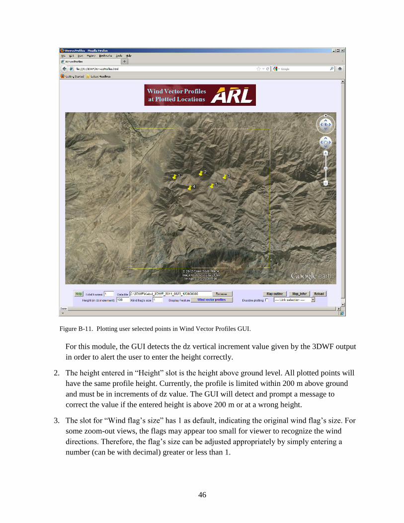
Figure B-11. Plotting user selected points in Wind Vector Profiles GUI.
For this module, the GUI detects the dz vertical increment value given by the 3DWF output
in order to alert the user to enter the height correctly.
2. The height entered in “Height” slot is the height above ground level. All plotted points will
have the same profile height. Currently, the profile is limited within 200 m above ground
and must be in increments of dz value. The GUI will detect and prompt a message to
correct the value if the entered height is above 200 m or at a wrong height.
3. The slot for “Wind flag’s size” has 1 as default, indicating the original wind flag’s size. For
some zoom-out views, the flags may appear too small for viewer to recognize the wind
directions. Therefore, the flag’s size can be adjusted appropriately by simply entering a
number (can be with decimal) greater or less than 1.
47
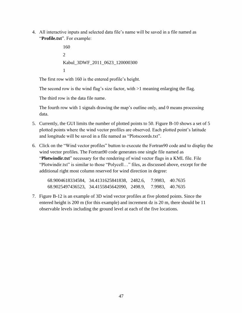
4. All interactive inputs and selected data file’s name will be saved in a file named as
“Profile.txt”. For example:
160
2
Kabul_3DWF_2011_0623_120000300
1
The first row with 160 is the entered profile’s height.
The second row is the wind flag’s size factor, with >1 meaning enlarging the flag.
The third row is the data file name.
The fourth row with 1 signals drawing the map’s outline only, and 0 means processing
data.
5. Currently, the GUI limits the number of plotted points to 50. Figure B-10 shows a set of 5
plotted points where the wind vector profiles are observed. Each plotted point’s latitude
and longitude will be saved in a file named as “Plotscoords.txt”.
6. Click on the “Wind vector profiles” button to execute the Fortran90 code and to display the
wind vector profiles. The Fortran90 code generates one single file named as
“Plotwindir.txt” necessary for the rendering of wind vector flags in a KML file. File
“Plotwindir.txt” is similar to those “Polycell…” files, as discussed above, except for the
additional right most column reserved for wind direction in degree:
68.9004618334584, 34.4131625841838, 2482.6, 7.9983, 40.7635
68.9025497436523, 34.4155845642090, 2498.9, 7.9983, 40.7635
7. Figure B-12 is an example of 3D wind vector profiles at five plotted points. Since the
entered height is 200 m (for this example) and increment dz is 20 m, there should be 11
observable levels including the ground level at each of the five locations.

48
Figure B-12. Wind vector profiles from the ground to 200 m height at 5 plotted locations.
8. The 3D wind vector flag is a rectangle-based pyramid with the top pointing to the direction
of the wind flow. The wind flag is not just for horizontal direction but also includes vertical
direction. Notice that since Google Earth’s point-of-focus is in the middle of the display
window, a zoom-in action will distort the straight up vertical line and wind flag’s direction
of other profiles that are not near the center of the display window. For this reason, the user
needs to pan the display window to place a profile location right at the center of the display
window in order to observe the wind direction correctly.
This GUI also allows multiple frames generation, as described previously.
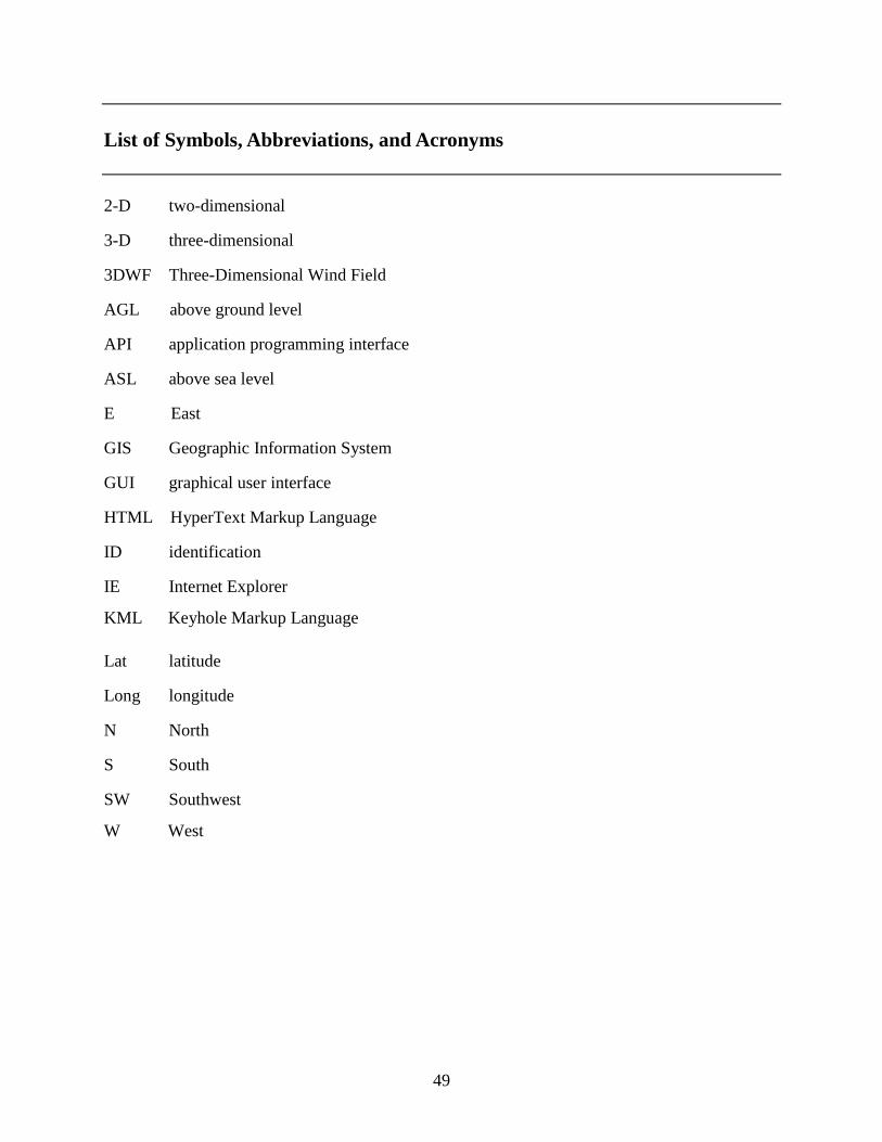
49
List of Symbols, Abbreviations, and Acronyms
2-D two-dimensional
3-D three-dimensional
3DWF Three-Dimensional Wind Field
AGL above ground level
API application programming interface
ASL above sea level
E East
GIS Geographic Information System
GUI graphical user interface
HTML HyperText Markup Language
ID identification
IE Internet Explorer
KML Keyhole Markup Language
Lat latitude
Long longitude
N North
S South
SW Southwest
W West

50
NO. OF
COPIES ORGANIZATION
1 ADMNSTR
ELEC DEFNS TECHL INFO CTR
ATTN DTIC OCP
8725 JOHN J KINGMAN RD STE 0944
FT BELVOIR VA 22060-6218
3 US ARMY RSRCH LAB
ATTN IMAL HRA
MAIL & RECORDS MGMT
ATTN RDRL CIO LL TECHL LIB
ATTN RDRL CIO LT TECHL PUB
ADELPHI MD 20783-1197
1 US ARMY RSRCH LAB
ELEC ATTN RDRL WML B J CIEZAK-JENKINS
BLDG. 390
ABERDEEN PROVING GROUND MD
21005-5069
8 US ARMY RESEARCH LAB
ATTN RDRL CIE D
G HUYNH (5 COPIES)
Y WANG
C WILLIAMSON
ATTN RDRL CIE P CLARK
ADELPHI, MD
6 US ARMY RESEARCH LAB
ATTN RDRL CIE D
D HOOCK (5 COPIES)
G VAUCHER
BLDG 1622
WHITE SANDS MISSILE RANGE
NM 88002-5501
TOTAL: 19 (2 ELEC, 17 HCS)