Visual Tracking for Intelligent Vehicle-Highway Systems

Christopher E. Smith1 Charles A. Richards2

chsmith@cs.umn.edu richards@cs.stanford.edu

Scott A. Brandt3 Nikolaos P. Papanikolopoulos1*

sbrandt@cs.colorado.edu npapas@cs.umn.edu1Artificial Intelligence, Robotics, and Vision Lab 2Stanford Vision Lab

Department of Computer Science 114 Gates Building 1AUniversity of Minnesota Stanford University4-192 EE/CS Building Stanford, CA 94305-9010

200 Union St. SEMinneapolis, MN 55455

3Department of Computer ScienceUniversity of Colorado-Boulder

Campus Box 430Boulder, CO 80309-0430

Accepted to the IEEE Transactions on Vehicular Technology

* Author to whom all correspondence should be sent.

Visual Tracking for Intelligent Vehicle-Highway Systems

Christopher E. Smith Charles A. Richards

chsmith@cs.umn.edu richards@cs.umn.edu

Artificial Intelligence, Robotics, and Vision Lab Stanford Vision Lab

Department of Computer Science 114 Gates Building 1A

University of Minnesota Stanford University

4-192 EE/CS Building Stanford, CA 94305-9010

200 Union St. SE

Minneapolis, MN 55455

Scott A. Brandt Nikolaos P. Papanikolopoulos*

sbrandt@cs.umn.edu npapas@cs.umn.edu

Department of Computer Science Artificial Intelligence, Robotics, and Vision Lab

University of Colorado-Boulder Department of Computer Science

Campus Box 430 University of Minnesota

Boulder, CO 80309-0430 4-192 EE/CS Building

200 Union St. SE

Minneapolis, MN 55455

ABSTRACTThe complexity and congestion of current transportation systems often produce traffic situationsthat jeopardize the safety of the people involved. These situations vary from maintaining a safedistance behind a leading vehicle to safely allowing a pedestrian to cross a busy street. Environ-mental sensing plays a critical role in virtually all of these situations. Of the sensors available,vision sensors provide information that is richer and more complete than other sensors, makingthem a logical choice for a multisensor transportation system. In this paper we propose robustdetection and tracking techniques for intelligent vehicle-highway applications where computervision plays a crucial role. In particular, we demonstrate that the Controlled Active Vision frame-work [15] can be utilized to provide a visual tracking modality to a traffic advisory system inorder to increase the overall safety margin in a variety of common traffic situations. We haveselected two application examples, vehicle tracking and pedestrian tracking, to demonstrate thatthe framework can provide precisely the type of information required to effectively manage thegiven traffic situation.

* Author to whom all correspondence should be sent.

1

1 Introduction

Transportation systems, especially those involving vehicular traffic, have been subjected to

considerable increases in complexity and congestion during the past two decades. A direct result

of these conditions has been a reduction in the overall safety of these systems. In response, the

reduction of traffic accidents and the enhancement of an operator’s abilities have become impor-

tant topics in highway safety. Improved safety can be achieved by assisting the human operator

with a computer warning system and by providing enhanced sensory information about the envi-

ronment. In addition, the systems that control the flow of traffic can likewise be enhanced by

providing sensory information regarding the current conditions in the environment. Information

may come from a variety of sensors such as vision, radar, and ultrasonic range-finders. The sen-

sory information may then be used to detect vehicles, traffic signs, obstacles, and pedestrians with

the objectives of keeping a safe distance from static or moving obstacles and obeying traffic laws.

Radar, Global Positioning System (GPS), and laser and ultrasonic range-finders have been pro-

posed as efficient sensing devices. Vision devices (i.e., CCD cameras) have not been extensively

used due to their high cost and noisy nature. However, the new generation of CCD cameras and

computer vision hardware allows for efficient and inexpensive use of vision sensors as a compo-

nent of a larger, multisensor system.

The primary advantage of vision sensors is their ability to provide diverse information on

relatively large regions. Simple tracking techniques may be used with visual data taken from a

vehicle to track several features of the obstacle ahead. This tracking allows us to detect obstacles

(e.g., pedestrians, vehicles, etc.) and keep a safe distance from them. Optical flow techniques in

conjunction with automatic selection of features allow for fast estimation of the obstacle-related

parameters, resulting in robust obstacle detection and tracking with little operator intervention. In

addition, surface features on the obstacles or knowledge of the approximate shape of the obstacles

(i.e., the shape of the body of a pedestrian or automobile) may further improve the robustness of

the tracking scheme. A single camera is proposed instead of a binocular system because one of

our main objectives is to demonstrate that relatively unsophisticated and uncalibrated off-the-shelf

2

hardware can be used to solve the problem. The ultimate goal of this research is to examine the

feasibility of incorporating visual sensing into an automated Intelligent Vehicle-Highway System

(IVHS) that provides information about pedestrians, traffic signs, and other vehicles.

One solution to these issues can be found under the Controlled Active Vision framework

[15]. Instead of relying heavily ona priori information, this framework provides the flexibility

necessary to operate under dynamic conditions where many environmental and target-related fac-

tors are unknown and possibly changing. The Controlled Active Vision framework utilizes the

Sum-of-Squared Differences (SSD) optical flow measurement [2] as an input to a control loop.

The SSD algorithm is used to measure the displacements of feature windows in a sequence of

images where the displacements may be induced by observer motion, target motion, or both.

These measured displacements are then used as one of the inputs into an intelligent traffic advi-

sory system.

Additionally, we propose a visual tracking system that does not rely upon accurate measures

of environmental and target parameters. An adaptive filtering scheme is used to track feature win-

dows on the target in spite of the unconstrained motion of the target, possible occlusion of feature

windows, and changing target and environmental conditions. Relatively high-speed targets are

tracked under varying conditions with only rough operating parameter estimates and no explicit

target models. Adaptive filtering techniques are useful under a variety of situations, including the

applications discussed in this paper: vehicle and pedestrian tracking.

We first describe some relevant previous research and present a detection scheme that

focuses on computational issues in a way that makes a real-time application possible. Next, we

describe our framework for the automatic detection of moving objects of interest. We then formu-

late the equations for measuring visual motion, including an enhanced SSD surface construction

strategy and efficient search alternatives. We also discuss a feature window selection scheme that

automatically determines which features are worthwhile for use in visual tracking. The paper con-

tinues with the presentation of the architecture that is used for conducting the visual tracking

experiments. Furthermore, we document results from feasibility experiments for both of the

3

selected applications. Finally, the paper concludes with a discussion of the aspects of the system

that deserve further consideration.

2 Previous Work

An important component of a real-time vehicle-highway system is the acquisition, process-

ing, and interpretation of the available sensory information regarding the traffic conditions. At the

lowest level, sensory information is used to derive discrete signals for a traffic or a vehicle system.

There are many potential high-level uses for information that these lower levels can provide. Two

common uses include automatic vehicle guidance and traffic management systems. For automatic

vehicle guidance, a computer system assists or replaces the human’s control of a vehicle. Traffic

management systems require the information for reporting a traffic incident and/or altering traffic

flow in order to correct the problem. In both of these cases, the system studies transportation con-

ditions in order to adjust the behavior of a global information or control system.

Information about the traffic can be obtained through a variety of sensors such as radar sen-

sors, loop detectors, and vision sensors. Among them, the most commonly used is the loop

detector. However, loop detectors provide local information and introduce significant errors in

their measurements. Recently, many researchers [7][8][10][11][12][16][18][20][22] have pro-

posed computer vision techniques for traffic monitoring and vehicle control. Waterfall and

Dickinson [21] proposed a vehicle detection system based upon frame differencing in a video

stream. Houghtonet al. [7] have proposed a system for tracking vehicles in video-images at road

junctions. Inigo [8] has presented a machine vision system for traffic monitoring and control. A

system that counts vehicles based on video-images has been built by Pellerin [16]. Kilger [11] has

done extensive work on shadow handling in a video-based, real-time traffic monitoring system.

Michalopoulos [12] has developed the Autoscope system for vision-based vehicle detection and

traffic flow measurement. A system similar to the Autoscope traffic flow measuring system has

been built by Takatooet al. [18]. This system computes parameters such as average vehicle speed

and spatial occupancy. A vision-based collision avoidance system has been proposed by Ulmer

4

[20]. Zielke et al. [22] have developed the CARTRACK system that automatically selects the

back of vehicles in images and tracks them in real-time. In addition, similar car-following algo-

rithms have been proposed by Kehtarnavazet al. [10]. Finally, several other groups [5][19] have

developed vision-based autonomous vehicles. In the remainder of this paper, we will highlight the

differences of these approaches with the approach our work has taken.

3 Detection and Tracking in a Traffic Vision System

In general, the satisfaction of the goal of constructing visual tracking modalities for intelli-

gent vehicle-highway systems requires the consideration of many elements. We have identified

four principal categories of IVHS vision components. These include the detection of traffic

objects of interest, the selection of features to be tracked, the tracking of features, and any motion

or object analysis.

3.1 Detection of Traffic Objects of Interest

One limitation of tracking using feature windows based upon Sum-of-Squared Differences

optical flow (see Sections 3.2 through 3.4) is that, by itself, there is no way of determining what

the tracked feature represents. Considering only a window of intensities, we could be looking at a

portion of a pedestrian, the edge of a building, a randomly-moving leaf, or a wide variety of other

items. Given an arbitrary image, the success of tracking an object such as a pedestrian relies on

the assumption that we somehow are able to detect that the tracked feature windows correspond to

the object in question. Some research projects involved with the study of motion avoid this issue

of detection by providing a human user with an interface for the selection of trackable features

[15]. However, if an intelligent vision system is to be able to robustly track traffic objects in

unpredictable, real-world environments, it is required that the system have some means of detect-

ing such objects automatically.

In considering detection, it is helpful to consider an image to be comprised of pixels that are

in one of two categories:figure or ground. Figure pixels are those which are believed to belong to

a traffic object of interest, while ground pixels belong to the objects’ environment. We consider

5

detection to be the identification and the analysis of figure pixels in each image of the temporal

sequence.

There is a wide variety of techniques that could be used for the identification of whether a

pixel is part of the figure or ground. For example, we could possess a model of the average shape

of automobiles and attempt to fit this model to locations within an image. However, identification

schemes that are computationally intensive may not be able to complete detection in real-time.

Using such schemes would cause the vision system to lack robustness. In searching for a fast

means to estimate the figure/ground state of a pixel, we consider the heuristic that uninteresting

objects (such as a sidewalk) tend to be displayed by pixels whose intensities are constant or very

slowly changing over time, while objects of interest (such as a pedestrian) tend to be located

where pixel intensities have recently changed. Thus, a comparison between images that occurred

at different times may yield information about the existence of important objects. This type of

frame differencing has a long history in vehicle detection [21]. The work of Waterfall and Dickin-

son [21], for example, proposed frame differencing as a means for detecting vehicles in a

sequence of images. Our system shares several ideas with their work, including a time averaged

ground image and a filter to reduce artifacts caused by camera noise. Because of the limitations of

processor speed when their work was published, they were unable to incorporate the filtering and

the time averaged ground image in their system [21]. We have also extended this type of detection

paradigm to include the use of detection domains, region merging, and post detection analysis

directed at eliminating non-traffic related objects. These extensions are detailed in the remainder

of this section.

The proposed scheme maintains aground image that represents the past history of the envi-

ronment. For each pixel in the current image, a comparison is made to the corresponding pixel in

the ground image. If they differ by more than a threshold intensity amount, then the pixel is con-

sidered to be part of a binaryfigure image. If this threshold is too small, then portions of the object

may blend into the background. If the threshold is too large, then slight changes in the environ-

ment will cause “false positive” errors in which the figure image contains many pixels that don’t

6

necessarily belong to important objects. A smaller, more sensitive threshold can be used if the

images are preprocessed with a low-pass filter. The filter spatially averages the pixels, making

camera noise cause smaller difference values. Experimentally, a 10% difference from a range of

256 grayscale intensity values was found to be a good general-purpose threshold level.

Figure 1 shows the construction of a figure image. The upper left window shows a portion of

a ground image that has been stored in memory. The upper right window shows a corresponding

portion of the current image. At the instant of time that was selected for this image, a pedestrian

had just begun crossing the street. The lower window shows how the pedestrian becomes readily

apparent, as the figure image is formed by comparing the current and the ground images.

Initially, the ground image is a copy of the first image of the sequence. However, environ-

mental changes (e.g., moving clouds and the corresponding shadows) may cause a pixel’s

Figure 1: Figure Image Construction

Ground Image

Current Input from the Camera

Resultant Figure Image

7

intensity to vary over time. To account for this dynamic aspect of IVHS environments, our system

periodically updates the ground image with information from the current frame of intensities.

Rather than periodically replacing the previous ground image, a new ground image is produced by

incorporating new intensity values from the current image according to:

(1)

where is theith ground image (i = k mod 3600), is the current image, and is

a scalar representing the importance of the current data. This equation refers to the intensities of a

specific pixel location in both the ground image and the current image.

Once a figure image has been obtained, we can consider the other activity of detection: ana-

lyzing the traffic objects that may be present in the figure image. However, figure images tend to

contain pixels that belong to a variety of items other than just the traffic objects of interest. For

example, one may find objects such as vehicles in the pedestrian tracking domain, regions caused

by shadows, and small areas of false detection caused by camera noise. The identification and

removal of many of these problem cases occurs as a beneficial side-effect of the partitioning of

figure pixels intosegments that each represent a traffic object.

The image figure segmentation is achieved through a single pass of the Sequential Labeling

Algorithm described in [6]. Because the algorithm creates segments from only a single pass

through the binary figure image, all statistics that are to be calculated for the segments must be

done dynamically. The selection of which statistics to calculate depends on the segment analysis;

for our purposes it suffices to maintain a size (pixel count) and a bounding box of the minimum

and maximum pixel locations in the two image dimensions (see Figure 2). There can be as many

as several hundred segments generated in a single image, only a few of which describe traffic

objects. Since the computational performance of object detection relies on keeping the number of

considered segments to a minimum, several pruning steps must be performed. In particular, a pass

is made through the segment data structure after each scanline is processed, during which many

segments are pruned away if they are found to have different dimensions than those of a typical

traffic object. In practice, this pruning removes almost all of the undesirable sources of figure

Gi 1 α–( )Gi 1– αIk+=

Gi Ik α 0 α 1≤ ≤( )

8

segments.

A common artifact that is observed with figure images is that objects will often be illumi-

nated in a way that causes a curve of background-matching intensities along the interior of their

projected area. For example, the arm of a pedestrian may sometimes be seen in the figure as two

adjacent halves. The result is a pair of segments whose bounding boxes overlap. Since these

curves are usually not parallel to an axis for their entire length, bounding box pairs caused by this

phenomenon almost always overlap. Thus, overlapping figure segments are merged into a single

bounding box, as illustrated in Figure 3.

Even though the figure/ground approach is a relatively fast form of object detection, its crit-

ical real-time nature is such that we would still like to identify ways in which the performance can

Figure 2: Segmentation Output

Figure 3: Segment Merging

9

be improved. One such method involves the use ofdomains. A domain is an individual, rectangu-

lar portion of the current image frame within which the segmentation algorithm is applied. Instead

of using a single domain that covers the entire image, time can be saved by the appropriate use of

several, smaller domains. The segments obtained from each domain are then combined into a

resultant object set.

In our approach, there are two types of domains,spontaneous andcontinuous. Spontaneous

domains are rectangular areas specified by a person as a part of configuring the system to a partic-

ular location. Spontaneous domains are placed where it is anticipated that a traffic object will

appear for the first time. For example, pedestrian tracking with spontaneous domains may work

best if the domains are placed close to the intersection of sidewalks and the boundaries of the

image. Continuous domains for detection with a particular image are generated automatically by

considering rectangular areas that are centered around the locations of segments in the previous

iteration of detection. The continuous domains have dimensions that cause them to have slightly

more pixels than the previously detected segments, in each dimension. Continuous domains allow

for the efficient detection of mobile traffic objects at times when they move away from the sponta-

neous domain locations. Since spontaneous and continuous domains may overlap and it would be

wasteful to perform segmentation repeatedly with the same pixels, intersecting domains are tem-

porarily merged in a way that is similar to the merging of intersecting figure segments, as

described above.

Once detected, the object of interest must be tracked. In the following sections, we describe

the visual measurements we use to select and track features. The measurements are based upon

the Sum-of-Squared Differences (SSD) optical flow [2].

3.2 Visual Measurements

Our goal is an IVHS sensing modality capable of measuring motion in a temporal sequence

of images. This section includes the formulation of the equations for measuring this motion. Our

vehicle and pedestrian tracking applications use the same basic visual tracking measurements that

10

are based upon a simple camera model and an optical flow measure. The visual measurements are

combined with search-specific optimizations in order to enhance the visual processing from

frame-to-frame and to optimize the performance of the system in our selected applications. Addi-

tionally, automatic selection of the features to be tracked is also based upon these equations for

measuring motion.

3.2.1 Camera Model and Optical Flow

We assume a pinhole camera model with a world frame, RW, centered on the optical axis. In

addition, a focal lengthf is assumed. A pointP = (XW, YW, ZW)T in RW, projects to a pointp in the

image plane with coordinates(x, y). We can define two scale factorssx andsy to account for cam-

era sampling and pixel size, and include the center of the image coordinate system(cx, cy) given in

frame FA [15]. This results in the following equations for the actual image coordinates(xA, yA):

. (2)

Any displacement of the pointP can be described by a rotation about an axis through the

origin and a translation. If this rotation is small, then it can be described as three independent rota-

tions about the three axesXW, YW, andZW [4]. We will assume that the camera moves in a static

environment with a translational velocity (Tx, Ty, Tz) and a rotational velocity (Rx, Ry, Rz). The

velocity of pointP with respect to RW can be expressed as:

. (3)

By taking the time derivatives and using equations (2) and (3), we obtain:

(4)

. (5)

We use a matching-based technique known as the Sum-of-Squared Differences (SSD) opti-

cal flow [2]. For the pointp(k–1) = (x(k–1), y(k–1))T in the image(k–1) wherek denotes thekth

xA

f XWsxZW-------------- cx+ x cx and yA

f YWsyZW-------------- cy+ y cy+= =+= =

dPdt------- T– R P×–=

utd

dx xTzZW--------- f

TxZW sx--------------– x y

syRxf

------------ fsx----- x 2sx

f-----+

Ry– ysysx-----Rz++= =

vtd

dy yTzZW--------- f

TyZW sy--------------– f

sy----- y2sy

f-----+

Rx x ysxf

----- Ry– xsxsy-----Rz–+= =

11

image in a sequences of images, we want to find the pointp(k) = (x(k–1)+u, y(k–1)+v)T. This

point p(k) is the new position of the projection of the feature pointP in imagek. We assume that

the intensity values in the neighborhoodN of p remain relatively constant over the sequencek. We

also assume that for a givenk, p(k) can be found in an areaΩ aboutp(k–1) and that the velocities

are normalized by timeT to get the displacements. Thus, for the pointp(k–1), the SSD algorithm

selects the displacement∆x = (u, v)T that minimizes the SSD measure

(6)

whereu,v∈ Ω, N is the neighborhood ofp, m andn are indices for pixels inN, andIk–1 andIk are

the intensity functions in images(k–1) and(k).

In theory, the exhaustive search of the areaΩ for an optimal SSD value is sufficient to visu-

ally track a particular feature window. In practice, however, there are three main problems that

must be considered. First, if the motion of a traffic object is rapid enough to cause its projection to

move beyond the bounds of the search area before the tracking algorithm is able to complete its

search, then the algorithm will fail. Second, if we increase the size of the areaΩ in an effort to

reduce the likelihood of the previous problem, the time required for an iteration of tracking

increases, possibly making the problem worse. Third, the image intensity values of the tracked

object may change as the object experiences effects such as occlusion, non-rigid motion, and illu-

mination changes.

The following section describes a method for addressing the first two problems. The method

resolves the conflicting goals of searching a large area and of minimizing computations.

Approaches are then discussed that improve the performance of the SSD search without requiring

the reduction of the search area size.

3.2.2 Dynamic Pyramiding

Dynamic pyramiding is a heuristic technique which attempts to resolve the conflict between

fast computation and capturing large motions. Earlier systems utilized a preset level of pyramid-

e p k 1–( ) ∆x,( )Ik 1– x k 1 )– m+( ) y k 1–( ) n+,( ) –[

m n, N∈∑=

Ik x k 1–( ) m u+ + y k 1–( ) n v+ +,( )]2

12

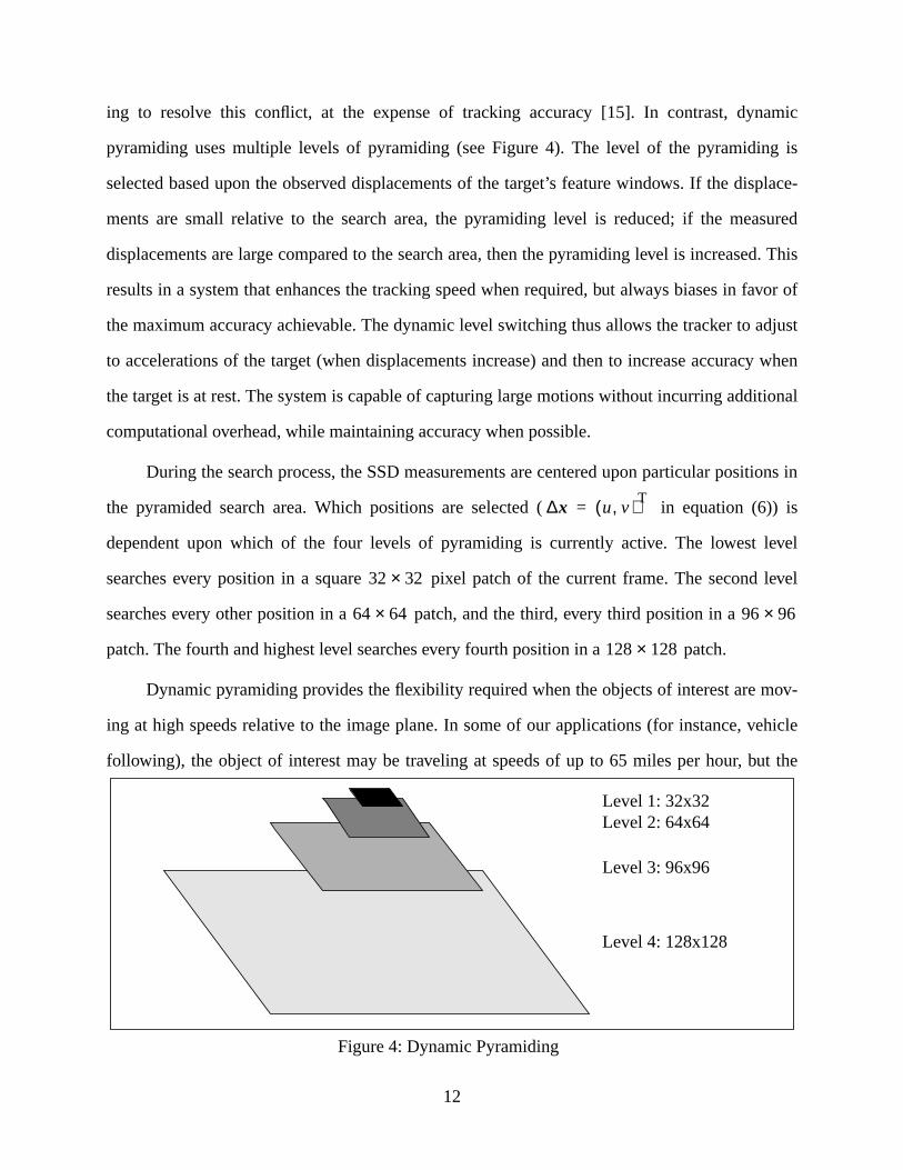
ing to resolve this conflict, at the expense of tracking accuracy [15]. In contrast, dynamic

pyramiding uses multiple levels of pyramiding (see Figure 4). The level of the pyramiding is

selected based upon the observed displacements of the target’s feature windows. If the displace-

ments are small relative to the search area, the pyramiding level is reduced; if the measured

displacements are large compared to the search area, then the pyramiding level is increased. This

results in a system that enhances the tracking speed when required, but always biases in favor of

the maximum accuracy achievable. The dynamic level switching thus allows the tracker to adjust

to accelerations of the target (when displacements increase) and then to increase accuracy when

the target is at rest. The system is capable of capturing large motions without incurring additional

computational overhead, while maintaining accuracy when possible.

During the search process, the SSD measurements are centered upon particular positions in

the pyramided search area. Which positions are selected ( in equation (6)) is

dependent upon which of the four levels of pyramiding is currently active. The lowest level

searches every position in a square pixel patch of the current frame. The second level

searches every other position in a patch, and the third, every third position in a

patch. The fourth and highest level searches every fourth position in a patch.

Dynamic pyramiding provides the flexibility required when the objects of interest are mov-

ing at high speeds relative to the image plane. In some of our applications (for instance, vehicle

following), the object of interest may be traveling at speeds of up to 65 miles per hour, but the

Level 1: 32x32Level 2: 64x64

Level 3: 96x96

Level 4: 128x128

Figure 4: Dynamic Pyramiding

∆x u v,( )T=

32 32×

64 64× 96 96×

128 128×

13

speed relative to the image plane is quite low. In other cases (e.g. pedestrian tracking or vehicle

lane changes), the speed of the object relative to the image plane may be quite high. In these

cases, dynamic pyramiding compensates for the speed of the features on the image plane, allow-

ing the system to maintain object tracking.

3.2.3 Loop Optimizations

We now consider a means of reducing tracking latency without decreasing the neighborhood

size. The primary source of latency in a vision system that uses the SS.D measure is the time

needed to identify the minimizing in equation (6). To find the true minimum, the SSD

measure must be calculated over each possible . The time required to produce a SSD sur-

face and to find its minimum can be greatly reduced by employing a loop short-circuiting

optimization. During the search for the minimum on the SSD surface (the search for ),

the SSD measure must be calculated according to equation (6). This requires nested loops for the

m andn indices. During the execution of these loops, the SSD measure is calculated as the run-

ning sum of the squared pixel value differences. If the current SSD minimum is checked against

the running sum as a condition on these loops, the execution of the loops can be short-circuited as

soon as the running sum exceeds the current minimum. This optimization has a worst-case perfor-

mance equivalent to the original algorithm plus the time required for the additional condition

tests. This worst case occurs when the SSD surface minimum lies at the last position

searched. On average, this type of short-circuit realizes a decrease in execution time by a factor of

two.

Another means for reducing latency for a given neighborhood size is based upon the heuris-

tic that the best place to begin the search is at the point where the minimum was last found on the

surface, expanding the search radially from that point. This heuristic works well when the distur-

bances being measured are relatively regular and small. In the case of tracking, this corresponds to

targets that have locally smooth velocity and acceleration. If a target’s motion does not exhibit

such relatively smooth curves, then the target itself is fundamentally untrackable due to the inher-

ent latency in the video equipment and the vision processing system.

u v,( )T

u v,( )T

u v,( )minT

u v,( )T

14

Under this heuristic, the search pattern in the image is altered to begin at the point on

the SSD surface where the minimum was located for the image. The search pattern then

spirals out from this point, searching over the extent ofu andv. This is in contrast with the typical

indexed search pattern where the indices are incremented in a row-major scan fashion. Figure 5

contrasts a traditional row-major scan and the proposed spiral scan where the center position cor-

responds to the position where the minimum was last found. This search strategy may also be

combined with a predictive filter to begin the search for the SSD minimum at the position that the

predictive aspect of the filter indicates to be the possible location of the minimum.

Since the structure that implements the spiral search pattern contains no more overhead than

the loop structures of the traditional search, worst-case performance is identical. In the general

case, search time is approximately halved.

We observed that search times for feature windows varied significantly — by as much as

100 percent — depending upon the shape/orientation of the feature and the direction of motion. In

determining the cause of this problem and exploring possible solutions, we realized that by apply-

ing the spiral image traversal pattern to the calculation of the SSD measure we could

simultaneously fix the problem and achieve additional performance improvements. Spiraling the

calculation of the SSD measure yields independence of best-case performance from the orienta-

tion and motion of the target by changing the order of the SSD calculations to no longer favor one

k( )

k 1–( )

Figure 5: Traditional and Spiral Search Patterns

15

portion of the image over another. In the traditional calculation pattern (a row-major traversal of

the feature region), information in the upper portion of the region is used before that in the lower

portion of the region, thus skewing the timing in favor of those images where the target and/or

foreground portion of the feature being tracked is in the upper half of the region and where the

motion results in intensity changes in the same region. Additional speed gains are achieved

because the area of greatest change in the SSD measure calculations typically occurs near the cen-

ter of the feature window, which generally coincides with an edge or a corner of the target,

resulting in fewer calculations before the loop is terminated in non-matching cases. Speed gains

from this optimization are approximately 40%.

3.2.4 Greedy, Gradient-Following Neighborhood Search

Both the traditional indexed search patterns and the above-described spiral search variations

perform an exhaustive computation over the feature window’s entire neighborhood. While this

exhaustive search is required in order to find the true SSD minimum, it may be desirable to sacri-

fice this guarantee in favor of expanding the search areaΩ while the search time is kept low. This

selects a point on the SSD surface that may not always be ideal, but can generally be found faster

than an exhaustive search in an expandedΩ. This is done by only computing SSD values on a

select few locations in the neighborhood, based on the SSD surface gradient information that pre-

vious computations may have provided. Imagine this search problem as one where you are

located on an uncharted three-dimensional terrain and the goal is to locate the lowest point. If

enough surface charting has taken place to indicate a depression, then it would make sense to con-

tinue charting in the direction of the depression. Further description of gradient-following search

strategies can be found in [3].

The greedy search optimization begins at a location within the SSD surface, and it consists

of a series of locally optimalgreedy decisions. Each decision computes the SSD values of neigh-

boring locations and selects the minimum. At the selected location, the same decision process is

repeated until no neighboring SSD value is better than the current one. However, this algorithm

provides no guarantees against instances of ridge, plateau, and foothill problems [3]. The greedy

16

searching optimization is typically able to compensate for the decrease in confidence in the

selected value by virtue of its speed.

3.3 Selection of Features to be Tracked

By computing a bounding box around a traffic object of interest (see Section 3.1), we have

reduced the problem of locating trackable features in the entire image to the problem of locating

trackable features in a smaller, rectangular region. We make the reasonable assumption that most

possible feature selections made from within a bounding box either lie entirely within the object

or contain at least a portion of the object’s pixels. By selecting several features for each object, we

increase the odds that we have a feature window on the object. Furthermore, our system tends to

select features that are near the center of the bounding box, an area with even greater likelihood of

being connected to the object.

But it is not enough to select any possible placement of a feature window within the bound-

ing box of a figure object. The reason for this is because a visual tracking algorithm based upon

the SSD technique may fail due to repeated patterns in the image’s intensity function or due to

large areas of uniform intensity. Both situations can provide multiple matches within a feature

window’s neighborhood, resulting in spurious displacement measures. In order to avoid this prob-

lem, our system considers and evaluates many candidate placements of a feature window.

Candidate placements which correspond to unique features are automatically selected.

The feature window selection uses the SSD measure combined with an auto-correlation

technique to produce a complete SSD surface corresponding to an auto-correlation in the areaΩ

[2][15]. Several possible confidence measures can be applied to the surface to measure the suit-

ability of a potential feature window.

The selection of a confidence measure is critical since many such measures lack the robust-

ness required by changes in illumination, intensity, etc. We utilize a two-dimensional

displacement parabolic fit that attempts to fit parabola to a cross-

section of the surface derived from the SSD measure [15]. The parabola is fit to the surface pro-

u v,( )T

e ∆xr( ) a∆xr2 b∆xr c+ +=

17

duced by equation (6) at several predefined orientations. A feature window’s confidence measure

is defined as the minimum of these directional measures.

Naturally, several candidate feature windows are tested and those which result in the best

confidence measures are kept. What remains to be discussed is the decision of which placements

of feature windows are used as candidates. The feature selection algorithm does this by using

another greedy, gradient-following search strategy. Depending on the number of desired resultant

feature window selections, several searches are begun at pre-determined locations within the

bounding box. A natural choice for at least one of these searches is the box’s center. Confidence

measures are computed for both the current candidate as well as for all the neighboring candi-

dates. As before, search continues from the neighbor with the best result, until no neighboring

confidence measures are better than the current one.

3.4 Feature Tracking and Motion Analysis

At this stage, the visual tracking system is provided with a set of features that it can track

according to the SSD optical flow method described earlier. The system performs several itera-

tions of the tracking phase, after which it returns to repeat the detection and selection steps. Thus,

the goal of tracking feature windows can be considered as that of providing feature trajectories

over time.

By advancing the capabilities of the IVHS visual tracking modality from the tracking of fea-

ture windows to the higher level of processing objects, we have provided the groundwork for a

variety of possible analysis tasks. Some tasks that have potential traffic-related applications

involve the identification of object characteristics such as the size of a pedestrian or the class of a

vehicle. Other tasks include the identification of motion characteristics such as a pedestrian’s gait

or the time that the person takes to traverse an intersection.

4 The Minnesota Vision Processing System

The purpose of this section is to describe the architecture on which we have developed our

visual tracking prototype. This description is intended to provide a justification for the way in

18

which our proposed algorithms address real-world constraints (e.g., complexity, accuracy, and

robustness).

The Minnesota Vision Processing System (MVPS) used in these experiments is the image

processing component of the Minnesota Robotic Visual Tracker (MRVT) [17] (see Figure 6). The

MVPS receives input from a video source such as a camera mounted in a vehicle, a static camera,

stored imagery played back through a Silicon Graphics Indigo, or a video tape recorder. The out-

put of the MVPS may be displayed in a readable format or can be transferred to another system

component and used as an input into a control subsystem. This flexibility offers a diversity of

methods by which software can be developed and tested on our system. The main component of

the MVPS is a Datacube MaxTower system consisting of a Motorola MVME-147 single board

computer running OS-9, a Datacube MaxVideo20 video processor, and a Datacube Max860 vec-

tor processor in a portable 7-slot VME chassis. The MVPS performs the image processing

computation and calculates any desired control input. It can supply the data or the input via shared

memory to an off-board processor via a Bit-3 bus extender for inclusion as an input into traffic or

vehicle control software. The video processing and calculations required to produce the desired

control input are performed under a pipeline programming model using Datacube’s Imageflow

Figure 6: MVPS Architecture

BIT3

M147

Max20

Datacube

Max860

VCR

SGI Indigo

Vehicle

StaticCamera

19

libraries.

The speed at which visual information can be processed is generally an important consider-

ation in the determination of the feasibility of computer vision systems. In the MVPS

configuration, portions of a vision application that cannot be directly implemented with

MaxVideo20 hardware elements can be programmed in software that runs on the Max860 proces-

sor. This processor has a peak performance rate of 80 Mflops. Communication between the

MaxVideo20 and the Max860 occurs at 20 Mhz through the use of the P2 bus.

5 Experimental Results

5.1 Pedestrian Tracking

Pedestrians constitute one class of trackable objects that are of extreme importance to many

IVHS applications. Considering the potential for injury when pedestrians and vehicles interact

harmfully, the ability to track pedestrians is likely to be an important element of any visual track-

ing system that is used for IVHS applications. Pedestrian tracking was therefore selected as the

first area to which our tracking paradigm was applied. In these experiments we consider the track-

ing of a pedestrian at an intersection by a static camera. By tracking pedestrians at intersections,

data can be collected regarding the existence of pedestrians in the crosswalk, the crossing time of

average pedestrians, and the identification of impaired pedestrians that cannot cross in the average

time frame. This information can be used for intelligent signal control that adapts to the time

required by impaired pedestrians to cross the street or for collaborative traffic/vehicle manage-

ment systems.

The goal of the first experiments was to demonstrate that our methods could successfully

track a pedestrian under normal environmental situations. The experiments consisted of a single

pedestrian crossing a street at a controlled intersection (See Figure 7). The camera was mounted

on the opposite side of the street in a position that was consistent with a mounting position on the

utility pole supporting the intersection’s crosswalk signals. Imagery was captured from a real

intersection using a camcorder and was later input into the MVPS using a video cassette recorder.

20

A single pedestrian crossed the street at the crosswalk, moving toward the camera (see Fig-

ure 8). Six example frames from a set of one hundred fifty frames of the pedestrian tracking

appear at the end of this paper (see Figure 14, at the end of this paper). The system tracked a fea-

ture on the pedestrian (the contrast gradient at the pedestrian’s waist). Target tracking was not lost

during the duration of the crossing, in spite of the degraded contrast in the imagery due to an over-

cast sky.

With the traditional application of optical flow tracking (described in Section 3.2.1), these

results would have been difficult. However, by combining the loop short-circuiting, the spiral pat-

tern for the search loop, and the spiral pattern for the SSD calculation loop (described in Section

3.2.3), we were able to find the minimum of an SSD surface as much as 17 times faster on the

average than the unmodified search. Experimentally, the search times for the unmodified algo-

rithm averaged 136 msec over 5000 frames under a variety of relative feature window motions.

The modified algorithm with the search-loop short-circuiting alone averaged 60-72 msec search

Figure 7: Experimental Setup

Figure 8: Pedestrian Tracking

TrackingBox

21

times over several thousand frames with arbitrary relative feature window motion. The combined

short-circuit/spiral search algorithm produced search times which averaged 13 msec under similar

tests and the combined short-circuit, dual-spiral algorithm produced search times which were as

low as 8 msec. Together these optimizations allow the MVPS to track three to four features at RS-

170 video rates (33 msec per frame) without video under-sampling. Subsequently, we applied the

gradient-following search scheme to sample image sequences and performance was found to be

similar to that for the combined short-circuit, dual-spiral algorithm.

The elements of the figure/ground system described earlier in the paper were implemented

with success, considering that this application is still in the early stage of development. Using the

pipeline image processing features of the Datacube MaxTower, the differencing between the cur-

rent and ground images was done at frame-rate. The segmentation of a single test object (200 by

300 pixels) in a complete image (512 by 480 pixels) took 150 msec. This time was clearly reduced

through the use of multiple, smaller domains. On an image sequence of several minutes of actual

pedestrian traffic on a sidewalk, the system successfully followed every pedestrian who entered in

the camera’s field of view. That is, no false negatives occurred for the duration of the experiment.

False positives did occur infrequently resulting in approximately 3% of the detections being

incorrect after the completion of the segment merging and object analysis. In general, these

occurred when a shadow of the traffic object fell on an object belonging to the ground image. One

advantage of using a figure image for tracking traffic objects is that the technique can track multi-

ple objects without a significant increase in computation. At the end of this paper there is a series

of illustrations that demonstrate how two bounding boxes produced by the segmentation of figure

images simultaneously track two pedestrians (see Figure 16).

The interaction between spontaneous and continuous domains substantially improved the

effectiveness of the detection phase. In Figure 9, the dynamic nature of the domains is illustrated.

First, the user selects two small domains at the ends of a sidewalk. Once the selection is made,

only a small area of the intersection’s projection is considered for segmentation of the figure

image. In the lower left window, we see that the segmentation has identified a pedestrian who has

22

approached from the left. The continuous domain around the discovered pedestrian is intersected

with the spontaneous domain that was already there. Finally, the lower right window shows the

pedestrian having moved away from the spontaneous domain, causing there to be three separate

Figure 9: Segmentation Domains

Original ImageUser selects spontaneous domains.

Spontaneous Domains

Pedestrian

Intersection of Non-intersecting Continuous DomainSpontaneous and Continuous Domains

Segmentation occurs here.

Initially, no segmentation occurs here.

Now, segmentation occurs at this location.

23

areas of figure segmentation.

5.2 Vehicle Tracking

A primary requirement of an intelligent vision system is that it must be able to detect and

track potential obstacles. Of particular interest are other vehicles moving around and in front of

the vehicle upon which the sensor is mounted (the primary vehicle). These vehicles constitute

obstacles that must be avoided (collision avoidance) or a target that is to be followed (convoying).

Collision avoidance of moving vehicles (with a relatively constant velocity) detected near

the primary vehicle can be effected with careful path planning. The basic goal is to maintain the

desired speed and path (i.e., staying in the same lane of the road or highway) while avoiding other

vehicles. Under normal circumstances this means accelerating and decelerating appropriately to

avoid cars in front of and behind the primary vehicle. In extreme cases this means taking evasive

action or warning the operator of a potential collision situation.

Another application area that involves the same basic problems is vehicle convoying. In this

case, all path planning is done by the operator of the vehicle at the head of the convoy and all

other vehicles must follow at a specified distance in a column behind the primary vehicle. For

these reasons we chose to apply the Controlled Active Vision framework to the problem of track-

ing vehicles moving in roughly the same direction as the primary vehicle.

The experimental data was collected by placing a camcorder in the passenger seat of a car

and driving behind other cars on the freeway (see Figure 10). This produced data that closely

matched that which could be expected in a typical IVHS application. This data was later played

back through a VCR and used as input to the MVPS, which tracked the vehicles and produced a

series of (x, y) locations specifying the detected locations of the features being tracked. Because

the exact world coordinate locations of the features in each frame of the video are unknown, we

were unable to provide a complete analysis of the tracking performance of the system. However, a

simple assumption about the motion of the vehicle in the frame yields conclusive results that

match the intuitive results gained from viewing the graphic display of the vehicle tracking

24

algorithm.

The MVPS includes a monitor upon which graphic representations of the tracking algorithm

are displayed. While the system is tracking, the input data is displayed and a red box is drawn

around the tracked location of the feature (see Figure 11). Initial experiments were done by

watching the system track the features as they were displayed on the monitor. This allowed us to

gain an understanding of the performance of the system under varying conditions and with a vari-

ety of features. In particular, we discovered that the performance of the system is very sensitive to

the robustness of the features selected.

After initial studies were completed, we proceeded to do a quantitative analysis of the vehi-

cle tracking performance. While we were unable to compare the tracking results against ground-

truth data (exact locations of objects/features manually calculated off-line), we were able to pro-

Figure 10: Experimental Setup

Tracking

Figure 11: Vehicle Tracking

Box

25

vide a reasonable determination of the system performance by assuming that the motion of the

vehicle within the frame would be relatively smooth and within easily determinable velocity

bounds. In other words, any sufficiently large, quick motions of the tracked location were likely to

be the result of a loss of tracking rather than due to motion of the vehicle. This hypothesis was

confirmed by viewing the tracking results and correlating the spikes in the plots of the tracked

locations with the motion of the displayed tracking windows.

Figure 12 shows the results of one such experimental run where a single feature (the license

plate) was tracked on the back of a single vehicle that was followed for approximately 2 minutes.

The plot on the left shows the motion of the feature in the frame with respect to a reference point

in the image that corresponds to an initial location of the feature. The plot on the right shows the

first derivative of the plot on the left. This plot clearly shows the relatively regular motion of the

calculated feature position, corresponding to the relatively smooth motion of the tracked vehicle

relative to the vehicle carrying the sensor. The spikes in the plot correspond to the times when the

tracking was lost and the tracking window rapidly moved off the feature. The plot has been anno-

tated to indicate the cause of the tracking problems, that in all cases were due to either momentary

occlusion of the tracked feature by windshield wipers on the primary vehicle, or extreme changes

in the relative brightness and contrast of the tracked feature as a result of the vehicles passing

under overpasses on the freeway. In all cases tracking resumed immediately after the visual distur-

500 1000 1500 2000 2500 3000 3500

10

20

30

500 1000 1500 2000 2500 3000 3500

10

20

30

40

50

60

Figure 12: Licence Plate Results

WindshieldOverpassesWipers

pixels

frames

pixels

frames

26

bance ended. In real-time this corresponded to less than a second of lost tracking per occurrence.

Simple filtering techniques (e.g., Kalman filtering) would effectively remove virtually all pertur-

bation of the tracking window resulting from such events.

Six selected frames of the test are presented in Figure 15 at the end of this paper. The image

labeled “(d)” is taken just prior to the loss of tracking due to windshield wiper occlusion. The blur

due to the wiper is just appearing in the lower left of the frame.

Figure 13 shows the results of tracking a different feature (the spoiler) on back of the same

vehicle tracked in the previous example. Tracking performance in this example is considerably

worse than in the previous example due to the poor SSD surface characteristics of the feature

selected by the operator. The tracking exhibits problems similar to the previous example, but

longer in duration and fails completely at about frame 2000. This failure corresponds to the algo-

rithm finding a suitable feature match on the surface markings of the freeway. Automatic feature

selection techniques presented earlier in this paper would not have chosen this feature for tracking

due to its poor SSD surface characteristics.

6 Drawbacks and Potential Extensions

In researching the MVPS, several limitations or future problems became apparent. Draw-

backs of relying solely upon the cross-correlated feature window tracking were previously

500 1000 1500 2000

10

20

30

40

500 1000 1500 2000

25

50

75

100

125

150

Figure 13: Spoiler Results

pixels

frames

pixels

frames

27

discussed, but the additional functions added to the visual system possess limitations as well. A

clear example of one of these is the sensitivity of the detection phase to jitter in the visual input

device. Unless the acquisition portion of the visual system contains sufficient stabilization abili-

ties, even slight jolts or gusts of wind have the ability to shift the placement of projected items of

the environment. This shifting causes large quantity of figure pixels along their borders. If we

properly tune the predication of a figure segment being an acceptable representation of a traffic

object of interest, then most of these large blobs of figure segments caused by camera jitter will be

properly ignored. However, two problems still remain. First, performance suffers due to the larger

number of pixels that are being processed at the time of the jitter. Second, objects that may other-

wise have been detected could have their bounding boxes intersected with those caused by jitter,

causing their undesirable removal.

Another concern that demands further research with the figure/ground approach is its depen-

dence on environmental conditions. Some conditions that would disturb humans, such as heavy

snowfall, would be ignored by the system (because each flake would be removed by the segmen-

tation size thresholds). A relatively frequent example of environmental effects on traffic vision

systems is that of cloud motion. Moving clouds can cause large, undesired regions in the figure

image due to sharp illumination changes. Currently, such regions are dealt with in the same man-

ner as those resulting from camera jitter.

Shadow handling is a common problem for most techniques that deal with the analysis of

moving objects. With visual tracking, shadows are one of several sources (in addition to non-rigid

motion, specular reflectivity, and others sources) for the variation in a feature window’s intensity

pattern. If this variation becomes too severe, the feature window will no longer be useful for esti-

mating the motion of its associated object of interest. Our system partially compensates for

shadows by continually switching between detection and tracking; however, the robust handling

of the effects of shadows continues to be an open problem and part of our ongoing research.

Another issue for further improvement is the update of the ground image through the time-

averaging process. Segmentation information can be used to increase the quality and the computa-

28

tional performance of the averaging. For example, information about the previous figure images

can be used to limit the scope of the averaging to those pixels that lie outside the figure image.

Occasionally a traffic object of interest will occlude something in the background in such a

way that corresponding colors for the two objects have hues that are clearly different to the human

observer, but whose intensity values are similar. Performing the differencing portion of obtaining

a figure image with more than just grayscale information may provide better results, but it adds

computational and hardware costs.

The performance of the pedestrian tracking could possibly be enhanced with the use of

explicit representations of people that are more complicated than simple bounding box con-

straints. A likely form would be to model a human as a semi-rigid body that deforms in known

and predictable ways. Such tracking would allow the system to track pedestrians in spite of rap-

idly changing conditions (i.e., the pedestrian moving from shadow to bright light) and clutter in

the image. Additionally, occlusion (due to a passing vehicle, other pedestrians, etc.) could be han-

dled more robustly than it currently is. The method presented here may be used to track multiple

features that in turn define the control points for a “snake,” or active deformable model, such as

has been described by Kass [9].

Since the largest source of latency in the figure/ground approach (as implemented on the

current hardware) lies in the switching between detection phase and the other phases, one might

consider tracking traffic objects based on a efficient connection between figure segments from

temporally adjacent frames. This would probably require the research of optimized correspon-

dence schemes that were specific to a particular IVHS task.

Finally, we should remember that a large-scale IVHS project would likely have a visual

tracking system as only one of many components. There are interesting challenges that deal with

the incorporation of the visual sensing data into larger, multisensor application systems for vari-

ous transportation applications.

29

7 Conclusion

This paper presents techniques for visual sensing in uncalibrated environments for intelli-

gent vehicle-highway systems applications. The techniques presented provide ways of recovering

unknown environmental parameters using the Controlled Active Vision framework [15]. In partic-

ular, this paper presents novel techniques for the automatic detection and visual tracking of

vehicles and pedestrians.

For the problem of visual tracking, we propose a technique based upon earlier work in

visual servoing [14][15] that achieves superior speed and accuracy through the introduction of

several performance enhancing techniques. The method-specific optimizations also enhance over-

all system performance without affecting worst-case execution times. These optimizations apply

to various region-based vision processing applications and, in our application, provide the

speedup required to increase directly the effectiveness of the real-time vision system.

Progress toward the goal of real-time processing for intelligent vehicle-highway systems

was also made by proposing means for performing other important visual motion tasks. A fast

strategy was described for the detection of areas that deserve continued processing. We then

showed how these areas of interest could then be used for the selection, tracking, and analysis of

feature windows. Experimentation confirmed the plausibility of a system that follows this type of

framework.

The application of these techniques to two selected IVHS problems has demonstrated the

feasibility of using a vision sensor to derive salient information from real imagery. The informa-

tion may then be used as an input into intelligent control or advisory systems. In such a system,

vision would constitute only one of the sensing modalities available to the system. Other sensors

such as radar, laser and ultrasonic range-finders, infra-red obstacle detectors, GPS, Forward Look-

ing Infra-Red (FLIR), microwave, etc. may provide other modalities with particular strengths and

weaknesses.

30

8 Acknowledgments

This work has been supported by the Minnesota Department of Transportation through Con-

tracts #71789-72983-169 and #71789-72447-159, the Center for Transportation Studies through

Contract #USDOT/DTRS 93-G-0017-01, the National Science Foundation through Contracts

#IRI-9410003 and #IRI-9502245, the Army High Performance Computing Research Center

under the auspices of the Department of the Army, Army Research Laboratory cooperative agree-

ment number DAAH04-95-2-0003/contract number DAAH04-95-C-0008 (the content of which

does not necessarily reflect the position of the policy of the government, and no official endorse-

ment should be inferred), the Department of Energy (Sandia National Laboratories) through

Contracts #AC-3752D and #AL3021, the McKnight Land Grant Professorship Program at the

University of Minnesota, and the Department of Computer Science of the University of

Minnesota.

9 References

[1] T. Abramczuck, “Microcomputer-based TV-detector for road traffic,” Seminar on Micro

Electronics for Road and Traffic Management, Tokoyo, Japan, October, 1984.

[2] P. Anandan, “A computational framework and an algorithm for the measurement of visual

motion,” International Journal of Computer Vision, vol. 2(3), pp. 283-310, 1988.

[3] M. Athans,Systems, Networks, and Computation: Multivariable Methods, McGraw-Hill,

New York, NY, 1974.

[4] J. Craig,Introduction to robotics: mechanics and control, Addison-Wesley, Reading, MA,

1985.

[5] E. Dickmanns, B. Mysliwetz, and T. Christians, “An integrated spatio-temporal approach to

automatic visual guidance of autonomous vehicles,”IEEE Transactions on Systems, Man,

and Cybernetics, vol. 20(6), pp. 1273-1284, November, 1990.

[6] B. Horn,Robot vision, MIT Press, Cambridge, MA, 1986.

[7] A. Houghton, G. Hobson, L. Seed, and R. Tozer, “Automatic monitoring of vehicles at road

junctions,”Traffic Engineering Control, vol. 28(10), pp. 541-453, October, 1987.

[8] R. Inigo, “Application of machine vision to traffic monitoring and control,”IEEE Transac-

tions on Vehicular Technology, vol. 38(3), pp. 112-122, August, 1989.

[9] B. Kass, A. Witkin, and D. Terzopoulos, “Snakes: Active contour models,”International

31

Journal of Computer Vision, vol. 1(4), pp. 321-331, 1987.

[10] N. Kehtarnavaz, N. Griswold, and J. Lee, “Visual control of an autonomous vehicle

(BART) — the vehicle-following problem,”IEEE Transactions on Vehicular Technology,

vol. 40(3), pp. 654-662, August, 1991.

[11] M. Kilger, “A shadow handler in a video-based real-time traffic monitoring system,” inPro-

ceedings of the IEEE Workshop on Applications of Computer Vision, 1992, pp. 11-18.

[12] P. Michalopoulos, “Vehicle detection video through image processing: the autoscope sys-

tem,” IEEE Transactions on Vehicular Technology, vol. 40(1), pp. 21-29, February, 1991.

[13] M. Okutomi and T. Kanade, “A locally adaptive window for signal matching,”International

Journal of Computer Vision, vol. 7(2), pp. 143-162, 1992.

[14] N. Papanikolopoulos, P. Khosla, and T. Kanade, “Visual tracking of a moving target by a

camera mounted on a robot: a combination of control and vision,”IEEE Transactions on

Robotics and Automation, vol. 9(1), pp. 14-35, 1993.

[15] N. Papanikolopoulos, “Controlled active vision,” Ph.D. Thesis, Department of Electrical

and Computer Engineering, Carnegie Mellon University, 1992.

[16] C. Pellerin, “Machine vision for smart highways,”Sensor Review, vol. 12(1), pp. 26-27,

1992.

[17] C. Smith, S. Brandt, and N. Papanikolopoulos, “Controlled active exploration of uncali-

brated environments,” inProceedings of the IEEE Conference on Computer Vision and Pat-

tern Recognition, 1994, pp. 792-795.

[18] M. Takatoo, T. Kitamura, Y. Okuyama, Y. Kobayashi, K Kikuchi, H. Nakanishi, and T. Shi-

bata, “Traffic flow measuring system using image processing,” inProceedings of SPIE,

1990, pp. 172-180.

[19] C. Thorpe, M. Hebert, T. Kanade, and S. Shafer, “Vision and navigation for the Carnegie-

Mellon NAVLAB,” IEEE Transactions on Pattern Analysis and Machine Intelligence, vol.

10(3), pp. 362-373, 1988.

[20] B. Ulmer, “VITA- an autonomous road vehicle (ARV) for collision avoidance in traffic,” in

Proceedings of the Intelligent Vehicles ‘92 Symposium, 1992, pp. 36-41.

[21] R. Waterfall and K. Dickinson, “Image processing applied to traffic, 2. practical experi-

ence,”Traffic Engineering and Control, vol. 25(2), pp. 60-67, 1984.

[22] T. Zielke, M. Brauckmann, and W. Von Seelen, “CARTRACK: computer vision-based car-

following,” in Proceedings of the IEEE Workshop on Applications of Computer Vision,

1992, pp. 156-163.

32

33

Figure 14: Pedestrian Tracking through Optical Flow

(a) (b)

(c) (d)

(e) (f)

34

35

Figure 15: Vehicle Tracking through Optical Flow

(a) (b)

(c) (d)

(e) (f)

36

37

Figure 16: Pedestrian Detection through Figure Segments

(a) (b)

(c) (d)

(e) (f)