visual navigation system for mobile robots

Technical report, IDE1130, June 2011

Visual Navigation System for

Mobile robots

Master’s Thesis in

Computer Science and Engineering

Badaluta Vlad

Embedded Intelligent Systems

Wasim Safdar

School of Information Science, Computer and Electrical Engineering

Halmstad University

Page i

Page ii

Visual Navigation System for

Mobile robots

School of Information Science, Computer and Electrical Engineering

Halmstad University

Box 823, S-301 18 Halmstad, Sweden

June 2011

Page iii

Page iv

Acknowledgement

Most of the fundamental ideas of science are essentially simple, and may, as a rule, be

expressed in a language comprehensible to everyone.

Albert Einstein

First of all we want to thank our supervisor Dr. Björn Åstrand, whose advice, suggestions and

experience helped us during the whole time of preparing and writing this thesis.

I, Vlad, would like to thank my coordinator from Romania, Dr. Remus Prodan, who has guided

me throughout my stay in Sweden.

I, Wasim, would specially like to thank my father Mr. Muhammad Safdar for helping me in my

hard times.

We would also offer our deep gratitude to our examiner Dr. Antanas Verikas for providing us the

opportunity to work on the thesis.

We also want to thank our families for providing us the possibility to study and trusting on our

capabilities.

Page v

Page vi

Details

First Name, Surname: Wasim Safdar

University: Halmstad University, Sweden

Degree Program: Embedded Intelligent Systems

Title of Thesis: Visual Navigation System for Mobile robots

Academic Supervisor: Dr. Björn Åstrand

First Name, Surname: Badaluta Vlad

University: Halmstad University, Sweden

Degree Program: Computer Science and Engineering

Title of Thesis: Visual Navigation System for Mobile robots

Academic Supervisor: Dr. Bjorn Åstrand

Abstract

We present two different methods based on visual odometry for pose estimation (x, y, Ө) of a

robot. The methods proposed are: one appearance based method that computes similarity

measures between consecutive images, and one method that computes visual flow of particular

features, i.e. spotlights on ceiling.

Both techniques are used to correct the pose (x, y, Ө) of the robot, measuring heading change

between consecutive images. A simple Kalman filter, extended Kalman filter and simple

averaging filter are used to fuse the estimated heading from visual odometry methods with

odometry data from wheel encoders.

Both techniques are evaluated on three different datasets of images obtained from a warehouse

and the results showed that both methods are able to minimize the drift in heading compare to

using wheel odometry only.

Keywords

Odometry, Appearance based model, Feature (spotlight) based model, Bayer’s pattern

Page vii

Page viii

Table of Contents

1 Introduction .................................................................................................................................... 1

1.1 Background ....................................................................................................................................... 1

1.2 Visual Navigation………………………………………………………………………………………………………………………..3

1.2.1 Visual Odometry .................................................................................................................. 3

1.2.2 Simultaneous Localization and Mapping…………………………………………………………………………3

1.2.3 Feature Extraction………………………………………………………………………………………………………....4

1.3 Problem Formulation…………………………………………………………………………………………………………………..6

2 Methods ......................................................................................................................................... 7

2.1 System Presentation ......................................................................................................................... 7

2.1.1 Sensing the environment ..................................................................................................... 9

2.1.2 Extraction of useful data from odometry……………………………………………………………………....9

2.1.3 Extraction of Useful data from visual odometry.................................................................9

2.1.4 Plotting pose of the robot.................................................................................................10

2.1.5 Testing and improvements of algorithms.........................................................................10

2.2 Data Evaluation...........................................................................................................................10

2.3 Demosaicing with Bayer’s Pattern..............................................................................................11

2.3.2 Bilinear Interpolation........................................................................................................12

2.4 Appearance based approach............. ........................................................................................13

2.4.1 Unwrapping.....................................................................................................................13

2.4.2 Rotation Estimation.........................................................................................................16

2.5 Spotlight detection and spotlight based turning correction system...........................................19

2.5.1 Spotlight Extraction..........................................................................................................19

2.5.2 Spotlight labeling.............................................................................................................20

2.5.3 Angle measuring for movement determination..............................................................21

Page ix

3 Experiments .................................................................................................................................. 23

3.1 Estimating robot path using Wheel Encoders................................................................................23

3.2 Minimum SSD and Outliners (Appearance Based Method)...........................................................25

3.3 Sensor Fusion using Extended Kalman Filter..................................................................................28

3.4 Sensor Fusion using Simple Kalman Filter and Extended Kalman Filter.........................................29

3.5 Sensor Fusion using Averaging Filter and Extended Kalman Filter................................................30

3.6 Decreasing FOV..............................................................................................................................31

3.7 Region of Interest for Spotlight Algorithm.....................................................................................32

4 Results and Discussions ................................................................................................................. 37

4.1 Preprocessing of Image...................................................................................................................38

4.2 Comparison of Odometry and Visual Odometry (Appearance Based Method)..............................38

4.3 Sensor Fusion with Extended Kalman Filter....................................................................................39

4.4 Sensor Fusion with Simple Kalman Filter and Exteneded Kalman Filter.........................................41

4.5 Sensor Fusion with Averaging Filter and Extended Kalman Filter...................................................43

4.6 Choosing optimal FOV.....................................................................................................................45

4.7 Values for angle for spotlight algorithm.........................................................................................47

5 Conclusion .................................................................................................................................... 49

References 51

Page x

Page xi

List of Figures

1. Step of robot navigation 8

2. Dataset 1 (a), Dataset 2 (b), Dataset 3 (c). 11

3. Bayer’s pattern 12

4. Green channel bilinear interpolation 13

5. Red channel bilinear interpolation 13

6. Blue channel bilinear interpolation 13

7. Omnidirectional camera view 14

8. Omnidirectional camera model 14

9. Unwrapping the Fish-eye image 15

10. Unwrapped Image 16

11. The front view of image is used to calculate heading of robot 17

12. Search widow 17

13. Euclidean distance between two consecutive images 18

14. Spotlight extraction unwrapped image 19

15. Spotlight extraction using threshold 19

16. labeling and identifying the spotlights in consecutive frames 20

17. Angle difference between consecutive frames 21

18. Spotlight angle calculation 22

19. Trajectory from odometry Dataset 1 24



22. The relative angle per frame from visual odometry (Dataset 1) 26

23. The plotting shows minimum SSD per frame (Dataset 1) 27

24. The plotting shows minimum SSD per frame (Dataset 2) 27

25. Steps in estimation of correct heading using Simple Kalman Filter 29

26. Steps in estimation of correct heading using AF and EKF 30

27. The red plotting shows minimum SSD per frame using FOV 7 degrees 31

and the blue plotting shows minimum SSD per frame using FOV 14

28. Plotting ROI 900 x 500 pixels(green) vs. odometry(blue) 33

29. Plotting ROI 1000 x 600 pixels (green) vs. odometry (blue) 34

30. Plotting ROI 1200 x 800 pixels (green) vs. odometry (blue) 34

31. Plottings ROI 1400 x 1000 pixels(green) vs. odometry(blue) 35

32. ROI plotting 35

33. Plotting of all the ROI values 36

34. Angle per frame from Visual odometry and odometry 39

35. Plot of Dataset 1 using Extended Kalman Filter 40

36. Plot of

Dataset 2 using Extended Kalman Filter 40

Page xii

37. Plot of Dataset 1 using SKF and EKF 42

38. Plot of Dataset 2 using SKF and EKF 42

39. Uncertainty measurement 44

40. Plot of Dataset 1 using Averaging Filter and Extended Kalman Filter 44

41. Plot of Dataset 1 using different sensor fusion algorithms 45

42. Heading correction using different FOV’s (Dataset 1) 46

43. Heading correction using different FOV’s (Dataset 2) 46

44. Plotting of the trajectory with constants 47

45. Graph of Sum of angles per frames 48

Page xiii

Page xiv

List of Tables

1. Dataset Properties 10

2. Experiments performed using different filters 23

Page xv

Page - 1 -

1

Introduction

In the past different researchers worked on visual navigation system for robots. They used

different visual sensors, different algorithms and sensor fusion for navigation system of robot.

1.1 Background

“Robots are the next big thing and the current state of the robot industry resembles the PC

industry 30 years ago”, said Bill Gates in the January 2007 issue of Scientific American [19].

Robots are intelligent agents that work on human command. Robots can perform tasks efficiently

that are difficult for human to perform.

The mobile autonomous robot is intelligently guided by the computer without human interfere.

Autonomous robots sense physical properties from the environment, extract features from the

sensors, build map and navigate through the path. The first autonomous robot was designed by

Walters (Essex) in 1948 [16]. Today the research in autonomous mobile robots increases day by

day. In fact autonomous robots are the focus of most of the industries. VOLVO is using

Automatic guided vehicle to transport motor blocks from one assembly to other [16]. BR 700

cleaning robot developed and sold by Kärcher Inc. Germany [17]. Its navigation system is based

on a very sophisticated sonar system and a gyro. HELPMATE is a mobile robot used in hospitals

for transportation tasks [18]. The autonomous mobile robots are also use for exploration, defense

and research purposes where it is difficult for human to reach and perform.

Page - 2 -

1. Introduction

Navigation is the most important task of any autonomous mobile robots. Accurate navigation

helps the robot to complete its task usually using GPS, sensors etc. The navigation based on

vision is becoming more and more important because of its large scope of applications. Different

types of sensors are used for visual navigation of mobile robots. The omnidirectional cameras are

gaining more and more importance in the automatic visual navigation because of their panoramic

view. These cameras give 360 degree view of field in single shot and it is easy to extract features

and navigate the robot in any environment. Alberto Ortiz [1] described systems that use visual

navigation is divided in different types depending on how they perceive knowledge from

environment.

Map-based navigation systems

Map-building based navigation systems

Map-less navigation systems

Behaviour Based navigation systems

Map-based navigation systems need the whole map of the environment before navigation starts.

The map is build by one sensor or combination of different sensors. The robot navigates through

the environment using the online data from the sensors and sensor fusion helps to correct the

robot pose. Map-building based navigation systems build the map by themselves and use this

map for navigation. This technique is also called simultaneous Location and Mapping (SLAM).

The robot explores the environment, build the map and use this map for navigation. Map-less

navigation systems do not need prior knowledge of the environment. The localization of the

robot is done by online invariant feature extraction or visual based navigation system. Behaviour

based navigation systems do not need map of the environment. Navigation is achieved by set of

filters that calculate different control variables of the robot. The collision detection and deadlock

avoidance is provided by one set of the sensors.

Page - 3 -

1.2. Visual Navigation

1.2 Visual Navigation

1.2.1 Visual Odometry

De Souza and Kak in [2] worked on indoor navigation and outdoor visual navigation. Chatila and

Laumond [3] describe procedure to combine information from the range finders and the camera

to build a map. Horn [4] and Lucas and Kanade [5] used optical flow based solutions to estimate

the motion of objects. Davison and Kita in [6] discuss about sequential localization and map

building. Lowe [6] developed SIFT (Scale invariant feature transform) method for tracking of

features from different views.

Dao [7] compute and use the homography matrix to detect and track the ground plane using

Harris Corner Detection. Davide Scaramuzza has done lot of research on visual navigation of

mobile robots. In [8] Scaramuzza presents visual odometry for ground vehicles using

omnidirectional camera. He represents two systems. One is guiding the vehicle on road using

SIFT features and RANSAC-based outlier removal to track key points on the ground plane. The

second is by using appearance-based approach. It is suggested that if scene points are nearly

collinear, they use Euclidean algorithm while in all other cases they use Triggs algorithm. Triggs

algorithm uses the homography based approach for planer motion while Euclidean algorithm

uses similarity measure between two consecutive image frames. Scaramuzza [8] proved from his

experiments that appearance-based approach is better than feature based approach for planar

motion of vehicle. In a second paper [9] Scaramuzza presents a descriptor for tracking vertical

line in omnidirectional images.

1.2.2 Simultaneous Localization and Mapping

Joel Hesch [10] describes SLAM (Simultaneous Location and Mapping) using omnidirectional

camera. The algorithm consists of image unwrapping, smoothing, edge detection and vertical

line detection. Range finders are used for localization and map building. Special landmarks are

Page - 4 -


detected by these rangefinders and localization and mapping is done by data association between

these landmarks and environment. Woo Yeon Jeong and Kyoung Mu Lee [11] proposed a new

vision-based SLAM (Simultaneous Location and Mapping) using both line and corner features as

landmarks in the scene. The proposed algorithm uses Extended Kalman Filter for localization

and mapping.

1.2.3 Feature Extraction

Fabien [12], worked on a visual navigation system using fluorescent tubes as landmarks. Their

method consists of two stages: an automatic map building system and secondly a navigation path

building system with orientation correction at the detection of a light (fluorescent tubes) that

were identified and recorded in the first step. The algorithm detects the fluorescent tubes, using a

fluorescent tube model (image thresholding, distortion correction, incomplete light elimination,

pose detection). When the robot gets near a light, which was recorded in the odometry system, it

takes a picture of the ceiling to estimate its approximate position and make position-adjustments.

Here they take advantage of the shape of the box in which the florescent lights are placed on the

ceiling, that restrict the lighting effect to a rectangle, so the navigation is based on the orientation

of the rectangle.

Hongbo Wang [13], has developed an similar algorithm to one from [11], meaning they are using

the same principle of the shape of the fluorescent lamps, except that here the lamps are the ones

that have orientation and the robot is dependent on identifying particular lamps. This means that

the lights are arranged on the ceiling in a certain pattern (matrix) knowing from the start the

positions of the lights in the real world.

1.2.4 Conclusion

The most common approach used by researcher is to find SIFT features and homography based

localization. We couldn’t use Laumond [3] method to combine laser information because this

information was not available for us, and we don’t have a reference point in respect to the

Page - 5 -


environment so is not enough for map building and localization. We use optical flow based

method for spot light navigation system. The Homography based technique Dao [7] is also very

good method for localization of robot. We can use this technique in future to improve our

algorithm. The localization of robot using SIFT features Lowe [6] is very good technique for

localization of robot but this needs precise calibration of camera and is effected by drifts in

trajectory. Francisco Bonin-Font [1] presents the detailed survey on visual navigation for mobile

robots. The paper describes different systems for land, aerial and underwater navigation systems.

After reading all these papers and after long discussion we concluded that we should use the

appearance based approach by Scaramuzza [8]. Scaramuzza compares different methods in his

paper and describes appearance based approach best because it is least affected by light and do

not need precise calibration of the camera. We are also going to experiment with a feature based

approach so that at the end, we have two methods developed that we can compare and combine

them to get an optimal result.

Page - 6 -

1.3. Problem Formulation

1.3 Problem Formulation

The objective of this thesis is to find suitable algorithm to correct the heading of robot by using

the visual odometry on the dataset available to us. The proposed methods will be evaluated

offline i.e. the whole data set is available before processing, but can be extended to an online

version.

The approach based on appearance based model assumes that scene points are nearly collinear,

camera undergoes pure rotation and camera is calibrated well. The real challenge is to find the

optimum algorithm or combination of different techniques to derive pose(x, y, Ө) of the robot

movement.

The problem in finding the best technique is divided in to three parts.

1. How to extract useful information.

The large dataset of images is available for offline evaluation. The type of data available

for the experiments and what kind of methods can be applied on this dataset have to be

checked and which visual odometry method gives us optimal results.

2. How to use the information for heading correction.

What algorithms and methods can be applied for heading correction of the robot and for

minimizing the processing time?

3. How to combine best techniques for improvement of algorithm.

What methods are used to combine the odometry data and visual odometry data in proper

way to get optimal results? The algorithms are tested on different datasets to evaluate the

feasibility and their performance.

Page - 7 -

2

Methods

2.1 System representation

The goal of our thesis is to find the best algorithm to correct the heading of the robot using visual

odometry. This heading correction can be later used to improve online navigation and

localization of the robot. The offline data available to us are the pictures taken from the fish-eye

camera from a warehouse, odometry data from wheel encoders and laser range sensors data. The

whole thesis is divided in to five parts as shown in the Fig. 1.

Page - 8 -

1. Methods

Figure 1: Step of robot Navigation

Figure 1: Step of robot Navigation

Plotting pose of the robot

Feature Extraction and visual

odometry using fisheye camera

Testing and Improvement of

algorithm

Real Environment

Sensing the environment

using different sensors

Extracting useful data from

odometry

Page - 9 -

2.1. System representation

2.1.1 Sensing the environment

The real environment in our case is warehouse sensed by a fish-eye camera, range sensors and

the wheel encoders. Odometry based on encoded data from wheels is used for making the

trajectory of the robot. The Odometry data is collected by Stage/Player in Linux. The data is

collected by these sensors is used for offline evaluation using different sensor fusion methods.

2.1.2 Extraction of useful data from odometry

The data available to us is from odometry for extracting information.

1 Odometry pose (x, y, θ) with timestamp

2 Images with timestamp

3 Laser information (Proximity data in meters) from laser scanner with time stamp.

2.1.3 Extraction of useful data from visual odometry

The information is extracted from the fisheye camera using methods based on visual odometry or

feature extraction. The two methods used by us for this purpose are:

1 Spot light based guiding navigation

2 Appearance based approach

The best method for visual navigation and heading correction is chosen by checking different

properties of the dataset available to us. The fish-eye images are taken from warehouse. The

warehouse consists of large paper reels. There are no distinct corners that will help the robot to

navigate.

Page - 10 -

1.1. Data Evaluation

2.1.4 Plotting pose of the robot

The information extracted from different methods is used for plotting the corrected pose of the

robot.

2.1.5 Testing and Improvements of algorithms

The trajectory is plotted by using different approaches based on different algorithms and tested

on different datasets.

2.2 Data Evaluation

The first part of the visual navigation is to evaluate the odometry data available to us. The data

set available to us are the panoramic images of the warehouse and odometry data. The odometry

data includes pose (x, y, θ) of robot from wheel encoders with timestamp. We have more than

5000 consecutive images in three distinct datasets. Table-1 shows dataset properties.

Dataset

No. Resolution No. of images Visual

odometry

Spotlights Figures

1 2050 x 2448 1894 X X (a)

2 2050 x 2448 976 X (b)

3 750x480 2157 X (c)

Table 1: Dataset Properties

Page - 11 -

2.3. Demosaicing with the Bayer Pattern

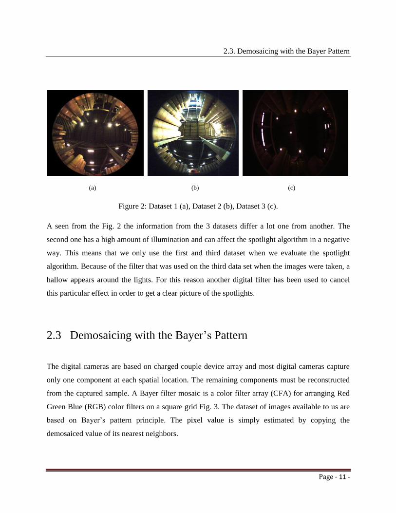
(a) (b) (c)

Figure 2: Dataset 1 (a), Dataset 2 (b), Dataset 3 (c).

A seen from the Fig. 2 the information from the 3 datasets differ a lot one from another. The

second one has a high amount of illumination and can affect the spotlight algorithm in a negative

way. This means that we only use the first and third dataset when we evaluate the spotlight

algorithm. Because of the filter that was used on the third data set when the images were taken, a

hallow appears around the lights. For this reason another digital filter has been used to cancel

this particular effect in order to get a clear picture of the spotlights.

2.3 Demosaicing with the Bayer’s Pattern

The digital cameras are based on charged couple device array and most digital cameras capture

only one component at each spatial location. The remaining components must be reconstructed

from the captured sample. A Bayer filter mosaic is a color filter array (CFA) for arranging Red

Green Blue (RGB) color filters on a square grid Fig. 3. The dataset of images available to us are

based on Bayer’s pattern principle. The pixel value is simply estimated by copying the

demosaiced value of its nearest neighbors.

Page - 12 -

2.3. Demosaicing with the Bayer Pattern

Figure 3: Bayer Pattern

2.3.1 Bilinear Interpolation

The average of each pixel is calculated depending on its position in Bayer’s Pattern [14]

in order to determine its spectrum. The interpolation of colors is calculated by equation 3.1, 3.2,

3.3 and 3.4

G 1 (3.1)

RC (3.2)

RS (3.3)

B1 (3.4)

See Fig. 4, Fig. 5 and Fig. 6

Page - 13 -

2.4. Appearance based approach

Figure 4: Green channel bilinear Interpolation

Figure 5: Red channel bilinear Interpolation

Figure 6: Blue channel bilinear Interpolation

2.4 Appearance based approach

2.4.1 Unwrapping

The first step is to unwrap the image into cylindrical panoramas for ease of processing. The

unwrapping is necessary so that image points become nearly collinear and we get linear

movement of pixels in front part of the view.

Page - 14 -


Panoramic images have horizontal angle up to 360 degrees and vertical angle up to 180 degrees

as shown in Fig. 7. In our case the fish-eye camera is mounted in an upward direction with z-axis

perpendicular to the ceiling as shown in Fig. 8.

Figure 7: Omnidirectional camera view

Figure 8: Omnidirectional Camera Model

We project pixel coordinates from the fish-eye image on a rectangular plane. We view the pixel

of the unwrapped circular image as polar coordinate system and each point of the image on the

plane is determined by the distance from fixed point and angle from fixed direction [15].

Page - 15 -


The polar coordinates are converted in to Cartesian coordinates using equation 3.5. This concept

is shown in Fig. 9.

x=r*cos (Ө), y=r*sin (Ө), where r = radius (3.5)

Figure 9: Unwrapping the Fish-eye Image

For experimental purpose we have the set of images in datasets available to us. We reduce the

image size by 50% before unwrapping the fish-eye image to save processing time. The reduction

of image size is not affecting the results in our experiments because of the high resolution of

images. We take the pixels from center of the fish-eye image considering the value of the radius

1 and then increasing it up to full length using equation 3.5. An example of an unwrapped image

is shown in Fig. 10.

Page - 16 -


Figure 10: Unwrapped Image. The blue marker represents front view of the image.

2.4.2 Rotation Estimation

To estimate the relative angle ΔӨ per frame, we use appearance based approach [8]. If the plane

of the camera is perfectly parallel to the ceiling’s plane then the pure rotation results in column-

wise shift of pixels in front view of the unwrapped image. The rotational angle could then be

retrieved by simply finding the best match between the reference image and the column-wise

shift of successive image after rotation. We only use the front view of robot for rotation

estimation because we are going forward in this part of unwrapped image pixel movement is

linear. The back portion of the image can be used as well if the robot goes backward. This is

shown in Fig. 11.

Page - 17 -

2.4. Appearance Based Approach

Figure 11: The front view of image is used to calculate heading of robot

A small search window is shifted from left to right and right to left in the captured image. We

changed the search window size in our experiments and we observed that results for rotation

estimation are good when the window size is small. The optimal size of our search window is

100x100 pixels, meaning field of view (FOV) that has been used is 14o. The SSD (Sum of square

differences) value for the search window is calculated between the reference image and shifted

image using equation 3.6. This SSD value gives us similarity measure between the consecutive

images. The search window is shown in Fig. 12.

Figure 12: The search widow is moved from right to left and left to right for rotation estimation.

The front view of the image is centered in this image.

Page - 18 -

2.4. Appearance Based Approach

The Euclidean distance between two appearances Ii and Ij (appearance means the search window

of the image) is measured using equation 3.6.

d(Ii,Ij,α)= (3.6)

where h is the image height, w is the image width, c represents the image color components. In

this case w is 2606 pixels, which means angular resolution is approx 7 pixels/о. The RGB color

space is used in this experiment. The minimum SSD is defined as a best similarity measure for a

search window as shown in Fig. 13. We get the number of pixels shifted (αmin) for best similarity

measurement. The rotational angle ΔӨ between two appearances Ii and Ij is calculated as seen in

equation 3.7.

ΔӨ= αmin /pixels per degree (3.7)

Figure 13: The Euclidean distance between two consecutive images. Image is shifted left by α

pixel to find best match.

Page - 19 -

2.5. Spotlight detection and spotlight based turning correction system

2.5 Spotlight detection and spotlight based turning correction

system

For this method the input data, meaning the images, haven’t been unwrapped because of the

distortion of the unwrapping algorithm at the extremities.

Figure 14: Spotlight extraction unwrapped image

As seen in Fig. 14 the spotlights are stretched at the top of the image and their trajectory is not

linear. That’s why, as it will be shown later, the region of interest that has been chosen in the

original image covers the area in which the spotlights have a linearly movement. In other words

this can be exploited for the determination of the best values for turns and forward movement.

2.5.1 Spotlight extraction

For spotlights detection, a threshold has been used, in order to get their position, see Fig. 15.

Figure 15: Spotlight extraction using threshold

Page - 20 -


First the region of interest is chosen (detecting the circular information from the image, as seen

in Fig. 15 the information that contains the spotlights (fisheye camera), after that a threshold has

been applied to extract the zones containing the spotlights. Knowing that the lights have the RGB

code close to 255, in dataset 1, we can apply a binary filter.

2.5.2 Spotlight labeling

For each new frame the spotlights have to be identified and labeled according to the positions of

the lights in the previous one, meaning tracking the ones that appear in both frames and finding

the new ones.

Figure 16: Labeling and identifying the spotlights in consecutive frames

The extraction of the spotlights is followed by their labeling as shown in Fig. 16. This process is

done for two consecutive frames in order to determine the new position of the same spotlights.

After extracting, identifying, labeling of the spotlights in the consecutive frames now comes the

process of finding which are located in both frames. The search for the same spotlights is

narrowed down to the zone surrounding the spotlights in the previous frame, thus creating

specific search zones with a specific search radius. These zones are further narrowed down using

Page - 21 -


an algorithm based on the last heading of each spotlight, meaning the search area is now

restricted to a sector of a circle.

2.5.3 Angle measuring for movement determination

After identifying the same spotlight, labeling the lights from consecutive frames the next step is

to calculate the difference of angles between the same spotlights.

Figure 17: Angle difference between consecutive frames

Page - 22 -


Based on these results a visual flow analysis will be done to determine the heading of the robot

in order to correct the angle of turning.

After getting the results from the experiments, the final angle is calculated by the following: after

the identification of a spotlight in two consecutive frames (as explained above), the angle

between the apparitions of those spotlights is measured. Following this an arithmetic mean is

calculated using all the angles of the identified spotlights see Fig. 17. From this point the value

of the angle is calculated by multiplying the mean with the constant 2 (value got from

experiments). Later after the optimal ROI is defined experiments with other constants will be

shown.

(3.8)

Using this formula on two different sets of data the same results have been obtained concerning

the angles in the turns and in the forward motion

Figure 18: Spotlight angle calculation

The angle of the heading of a specific spotlight is determined by subtracting angle a out of

angle b as shown in Fig. 18. This process of updating the heading is repeated every time the

spotlight is detected in consecutive frames.

Page - 23 -

3

Experiments

The experiments done on three distinct image datasets can be organized as shown in Table-2.

Experiments

No Heading Correction

Methods

Datasets Visual

Odometry

Spotlights

1 Extended Kalman Filter 1,2,3 X X

2 Simple Kalman Filter+EKF 1,2 X

3 Averaging.filter+ EKF 1 X

Table.2 Experiments performed using different filters (EFK, SK-EFK, AV-EFK)

3.1 Estimating robot path using Wheel Encoders

The data collected from visual odometry such as relative rotational angle ΔӨ and SSD per frame

is used for estimating robot path. We also have data from odometry that is used for making

trajectory of path followed by the robot. The odometry data is collected on real-time by using

stage/player [20] in Linux. These tools allow controlling the robot using any language, providing

network interface to any type of hardware and help to get extract information from odometry.

Player supports multiple concurrent client connections to devices, creating new possibilities for

distributed and collaborative sensing and control. The trajectory from 2-D position (x, y) from

odometry data taken from dataset 1, dataset 2 and dataset 3 is shown in Fig. 19, Fig. 20 and Fig.

21. The red circles represent missing data or jumps from odometry. The ground truth for our

Page - 24 -

3. Experiments

experiments is that the trajectory should be in a loop and angles at turn should be closer to 90

degree if the heading is correct. We will see later how to correct the odometry data so we get

correct heading. We used appearance based method [11] as opposed to feature-based method.

Figure 19: Trajectory from odometry Dataset 1. Red dots represent missing data or jumps.

Figure 20: Trajectory from odometry Dataset 2. Red dots represent missing data or jumps.

Page - 25 -

3.2. Minimum SSD and Outliners

Figure 21: Trajectory from odometry Dataset 3.

3.2 Minimum SSD and Outliners (Appearance Based Method)

The relative angle ΔӨ calculated from visual odometry using equation 3.7 is used to plot the

visual odometry trajectory. The graph in Fig. 22 shows relative angle per frame for all the fish-

eye images from dataset 1 calculated using appearance based method. The bumps in this graph

show turns in the robot path.

Page - 26 -

3.2. Minimum SSD and Outlines

Figure 22: The relative angle per frame from visual odometry (Dataset 1). Red circle shows turn

in path.

The minimum SSD value calculated for each for dataset 1 and dataset 2 is shown in Fig. 23 and

Fig. 24. This graph represents similarity level of each relative frame. The red dot with blue

circles represents outliners. This erroneous data is either because of jumps or abnormal frame

and it introduces outliners.

Page - 27 -

3.3. Minimum SSD and Outlines

Figure 23: The plotting shows minimum SSD per frame (Dataset 1). Blue circles are outliers

defined as values above 4500 mainly caused by jumps in data see Fig. 19.

Figure 24: The plotting shows minimum SSD per frame (Dataset 2). Blue circles are outliers

defined as values above 6000 mainly caused by jumps in data see Fig. 20.

Page - 28 -

3.3. Sensor Fusion using Extended Kalman Filter

3.3 Sensor Fusion using Extended Kalman Filter

In our experiments we get the robots 2-D position (x, y) from odometry and ΔӨ from the visual

odometry. To plot the heading from visual odometry we use extended kalman filter. The

predicted (priori) state in equation 3.9.

= + (3.9)

where is relative distance from odometry and is the relative angle from visual odometry.

The predicted (a priori) estimate covariance is equation.3.10.

(3.10)

whereas and

The updated (posteriori) state estimate is

(3.11)

Page - 29 -


whereas is Kalman gain and is innovation

covariance and is measurement residual.

(3.12)

(3.13)

(3.14)

3.4 Sensor Fusion using Simple Kalman Filter and Extended

Kalman Filter

Figure 25: Steps in estimation of correct heading using Simple Kalman Filter.

A careful study of SSD values from the graph in Fig. 23 and Fig. 24 we came to know

that SSD is increased above normal value if there is a jump in heading. This is also shown by

blue circles. The estimation of correct heading either from odometry or visual odometry is done

using simple kalman filter [11]. The SSD value is normalized so that linear extrapolation is

better. The heading correction is done using equation 3.15.

Page - 30 -

3.5. Heading Correction using Averaging Filter.

= (3.15)

Where SSD*= (SSD-thr_SSD)/thr_SSD.

The is angle from odometry, is visual odometry calculated angle and is

interpolated visual odometry angle. The thr_SSD is thresholded SSD value. This value represents

abnormality in heading.

3.5 Sensor Fusion using Averaging Filter and Extended Kalman

Filter

Figure 26: Steps in estimation of correct heading using averaging filter abd Extended

Kalman Filter.

The heading is corrected using averaging filter before updating the heading from

extended kalman filter. The averaging filter simply gives equal weights to some values of both

odomtery data and visual odometry data after there is jump in the heading as in equation 3.16.

The jump in the heading is known by observing the SSD value. The is the abnormal

SSD value after jump and found by experiments.

Page - 31 -

3.6. Decreasing FOV

= (3.16)

3.6 Decreasing FOV

Decreasing FOV from 14 degrees to 7 degrees doesn’t improve the results. Decreasing

ROI means that we are using more correct information but the area of search is decreased. There

are less information in the center of fish-eye image means at radius 1 and information increase as

you go towards boundary. The increase in FOV up to optimal value increases accuracy. The

decrease in FOV doesn’t improve the results for similarity measure of images. The minimum

sum of SSD value for each frame using same dataset and FOV 7 degrees is shown in Fig. 27.

Figure 27: The red plotting shows minimum SSD per frame using FOV 7 degrees and the blue

plotting shows minimum SSD per frame using FOV 14.

Page - 32 -

3.7. Region of Interest for spotlight algorithm

3.7 Region of Interest for Spotlight Algorithm

Experiments have been done with different sizes of the region of interest in order find the

optimal parameters in which the algorithm works. The center of the ROI is the same with the

center of the images, only the width and the height of it are modified in order to apply the

algorithm. In other words these parameters are shifted to see how much of the information in the

vicinity of the center affect the final output of the algorithm.

The following experiments have been done to determine the optimal values of the parameters

(image width and image height).

a. 900 x 500 pixels

Starting from this size the algorithm is beginning get positive results, meaning the trajectory

starts to resemble with the odometry information, see Fig. 28.

The next graph shows a comparison between the trajectory generated by the information

gathered from the odometry (Blue) and from the spotlight algorithm with the mentioned ROI

resolution (Green).

The trajectory of the spotlights that pass in this ROI is straight but their number is too small in

order to get an accurate measurement of the angles, especially in turns, as it’s seen in the graph

below.

Page - 33 -


Figure 28: Plotting ROI 900 x 500 pixels(green) vs. odometry(blue)

b. 1000 x 600 (Height ratio = 0.571; Width ratio = 0.342)

For this particular size, the algorithm got the best plotting of the trajectory. This has been

achieved by gaining more information from the spotlights, meaning more spotlights pass in the

ROI, but sacrificing the linearity trajectory of the spotlights at the left and right borders. This

does not affect the final results because the height of 1000 pixels enables the algorithm to take in

consideration the spotlights that are further away (front and back) that have an linearity trajectory

when the movement is forward orientated. In case of turning the spotlights that are nearby the

center have a smaller movement than the ones at the extremities of the height (the angular speed

is smaller), that can be approximated to and Euclidian linearity trajectory Fig. 28.

In the parts of the data that don’t contain large jumps, the algorithm got better results.

The 90 degrees turns are plotted correctly as well as the forward motion, except for the very big

jumps that appear in the data flow of the images, and the distances read from the odometry

system, see Fig. 29.

Page - 34 -


Figure 29: Plotting ROI 1000 x 600 pixels (green) vs. odometry (blue)

c. 1200 x 800

At this size of the ROI the forward motion is still detected in acceptable numbers, but the

turnings start to be erroneous Fig. 30.

Figure 30: Plotting ROI 1200 x 800 pixels (green) vs. odometry (blue)

Page - 35 -


d. 1400 x 1000

From this point there are errors in both forward motion and turnings Fig. 31.

Figure 31: Plottings ROI 1400 x 1000 pixels(green) vs. odometry(blue).

In Fig. 32 the four ROI’s that have been used are shown.

Figure 32: ROI plotting (Red - 900x600, Green - 1000x600,

Purple – 1200x800, Blue – 1400x1000).

Page - 36 -

3.7. Region of Interest for spotlight algorith

The next graph represents the plotting of all the trajectories with the different ROI values.

Figure 33: Plotting of all the ROI values.

As seen from the experiments Fig. 33 the best result was achieved with a region of interest of

1000 pixels height and 600 pixels width. (height ratio of 0.571, and width ratio = 0.342)(green

plotting).

Page - 37 -

4

Results and Discussions

The results based on the appearance based methods and spotlight based methods using different

sensor fusion filters (EFK, SK-EFK, AV-EFK), FOV’s and ROI are discussed here.

Assumptions in appearance based approach:

The assumptions chosen in appearance based model are

The robot goes pure horizontal rotation

It is assumed that there is no vibration and camera is moving parallel plane with

the ceiling.

The scene points are nearly collinear

It is assumed that pixel movement is nearly Euclidean when robot moves. Also

there is always small drift present but it has very little effect on our readings.

The camera is calibrated well

It is assumed that camera is precisely calibrated

Image size reduction

The reduction in size of image is not affecting our results. The image size is

reduced 50% to increase processing time

Page - 38 -

4. Results and Discussion

4.1 Preprocessing of Image

We have large set of data. The preprocessing of image data is compulsory to processing time for

results evaluation. The image also contains noise. Demociasing with Bayer’s pattern covert the

image into RGB format and also do act as smoothing filter because it calculates interpolated

values. The image preprocessing, doesn't have a dramatic impact upon the overall result, due to

the images high resolution. The digital camera captures only one component of the image. The

remaining color components are reconstructed using demosaiced value of their nearest

neighbours (see chapter 2.3). The conversion of image in to RGB image is necessary so that we

have more information about color components for measuring similarity measure of consecutive

images. The similarity of images is measured for three color components R, G and B. This

increases accuracy of our results.

4.2 Comparison of Odometry and Visual Odometry

(Appearance Based Method)

The useful information from the odometry data for our experiments is relative position and angle

of the robot. The odometry data is based on information collected from wheel encoders using

Stage/Player tool. The appearance based method (see chapter 2.4.2) is also used to measure

relative rotational angles using similarity measure between consecutive images. The difference

between these two sets of data means sum of angles from odometry and sum of angles from

appearance based method is shown in Fig. 34. The cyan represents data extracted from odometry

and red color represents data extracted from visual odometry. The total angle from odometry is

788 degrees while from visual odometry is 687 degrees. The difference between them is 101

degrees. Visual odometry value is underestimated and odometry value is overestimated. Both

Page - 39 -


measurements have errors because there are large jumps and drift in odometry data, also missing

images where there is a jump.

Figure 34: Angle per frame from Visual odometry and odometry. Red color represents visual

odometry data and cyan color represents odometry data.

4.3 Sensor Fusion with Extended Kalman Filter

The state xi of the robot is updated by predicted state of robot. We observe from the Fig.

38, when there is jump in trajectory the heading (x, y, Ө) becomes worse. When there is a jump

we have no information about robot pose. For heading calculation we use only Extended Kalman

Filter. The dataset 1 shows some improvement in trajectory at the start as shown in Fig. 35 but

after jump the estimation goes wrong. The dataset 2 also shows some improvement in the

trajectory when the robot goes forward as shown in Fig. 36.

Page - 40 -


Figure 35: Plot of Dataset 1 using Extended Kalman Filter. (Blue – odometry, Green – EFK).

Figure 36: Plot of Dataset 2 using Extended Kalman Filter. (Blue – odometry, Green – EFK).

Page - 41 -

4.4. Sensor Fusion with Simple Kalman Filter and Extended Kalman Filter

4.4 Sensor Fusion with Simple Kalman Filter and Extended

Kalman Filter

The heading is plotted using sensor fusion technique based on the Simple Kalman Filter and

Extended Kalman Filter (see chapter 3.4) for dataset 1 and 2. The angle measured using

appearance based approach is replaced with the angle measured from odometry when the SSD

value is greater than the specified threshold. We always get different SSD threshold values for

different datasets because of change of the amount of light in the environment. The threshold

SSD value for the first dataset after a jump is 4500 and for second dataset is 6000. The corrected

pose from the filter is used to plot. The Extended Kalman Filter estimates the heading of the

robot using 2-D position from odometry data. The Fig. 37 and Fig. 38 show that the heading is

not recovered using this approach. Only dataset 1 shows some improvement in trajectory because

we are using only front view of unwrapped image and in dataset 2 the estimation of the robot

pose goes wrong, it will be observed in Fig. 38.

Page - 42 -

4.4. Sensor Fusion with Simple Kalman Filter and Extended Kalman Filter

Figure 37: Plot of Dataset 1 using SKF and EKF.

Figure 38: Plot of Dataset 2 using SKF and EKF.

Page - 43 -

4.4. Sensor Fusion using Averaging Filter and Extended Kalman Filter

4.5 Sensor Fusion with Averaging Filter and Extended Kalman

Filter

We observe from Fig. 23 that when we have jump in heading we get high SSD value. This high

SSD value is shown by red dots. When we get SSD value greater than specified threshold in our

case it is 4500 we give equal weight to 10 to 15 values of both odometry and visual odometry

data. The time stamps between jump tells us that there are 10 to 15 missing frame per jump but

for last jump we have more than 25 missing frames. If we take mean of more than 25 frames our

trajectory become good for last jump but become worse for all other jumps because now we are

also changing correct heading. We take the mean of values from odometry and visual odometry

one by one and give equal weight to both odometry and visual odometry values as in equation

3.15. We use this filter because visual odometry underestimate the value and odometry

overestimate the value after jump. We know that they are near to correct estimation therefore we

applied averaging filter after jump. The values we get from this are always near to correct value

and are more precise see Fig. 39. We update the heading again using averaging filter with

extended kalman filter in equation 3.15. The graph in Fig. 40 shows that using this method the

heading is corrected very much and the second loop is exactly on the first loop. The heading after

second last jump is not improved due to very big jump and lot of missing data. This jump is

about 16 meters.

Page - 44 -

4.4. Sensor Fusion using Averaging Filter and Extended Kalman Filter

Figure 39: Uncertainty measurement

Figure 40: Plot of Dataset 1 using Averaging Filter and Extended Kalman Filter

The comparison of sensor fusion using Extended Kalman Filter, Simple Kalman Filter and

Extended Kalman Filter, Averaging Filter and Extended Kalman Filter is shown in Fig. 41. The

best result is obtained from using averaging Kalman Filter and Extended Kalman Filter.

Page - 45 -

4.6. Choosing FOV

Figure 41: Plot of Dataset 1 using different sensor fusion algorithms.

4.6 Choosing optimal FOV

The FOV for the similarity measure is chosen such that it will give optimum results. The middle

portion of the image marked by blue marker represents front portion of corridor, see Fig.10.

These pixels are mapped on upper portion of rectangular window. The upper part of unwrapped

image has less information. The information about the environment increases as we go down in

rectangular window. Therefore we consider the lower part of unwrapped image. The best vertical

and horizontal FOV selected is 14 degrees. The result obtained after choosing this FOV 14 and

FOV 7 for dataset 1 and 2 is shown in Fig. 42 and Fig. 43.

Page - 46 -

4.6. Choosing FOV

Figure 42: Heading correction using different FOV’s (Dataset 1).

Figure 43: Heading correction using different FOV’s (Dataset 2).

Page - 47 -

4.7. Values for angle for spotlight algorithm

4.7 Values for angle for spotlight algorithm

The first value used for the equation 3.8 is 1.9, see Fig. 44. As seen below this dramatically alters

the trajectory of the second turn. At the same time the forward heading is altered as well. So for

this value we don’t get the best correction.

Figure 44: Plotting of the trajectory with const. 1.9. (Red), 2.0 (Green), 2.1 (Black)

In the case of using a constant with the value 2.1 the angles in the turns become worse but the

forward heading remains unaltered.

Fig. 45 presents the graph of sum of angles per frames. The blue graph represents the angles

extracted from odometry, and the red one is the graph representing the angles generated with the

spotlight algorithm.

Page - 48 -

4.7. Values for angle for spotlight algorithm

The odometry angles have a peak of approx. 790 degrees. In reality because of the two loops on

the same path the angle should be 720 degrees. On the other hand the spotlight algorithm has an

output of approx. 690 degrees, the difference being only of 30 degrees.

As shown in the “stepped ladder” graph the constant values represent moving forward

and the differences / distances between the “steps”, the turnings.

Figure: 45: Graph of Sum of angles per frames (Blue – Odometry based angles, Red – Spotlight

algorithm based angles).

Page - 49 -

5

Conclusion

In this work, two different visual odometry methods for heading correction have been proposed:

an appearance based method and a spotlight navigation method. The derived heading from these

methods has been fused with odometry data from wheel encoders for better estimation of the

robot path. The evaluation of the performance and feasibility of the proposed methods have been

tested using three different datasets from warehouse using different:

– fusion methods (EFK, SK-EFK, AV-EFK)

– field of view (Appearance based method)

– region of interests (Spotlight method)

The limitations in correcting the pose of the robot in our project are followings.

Jumps and Missing images

There is missing information (jumps) in odometry data and also missing

images at those particular locations and in random places as well. These

jumps make it difficult to estimate correct heading of the robot.

Page - 50 -

5. Conclusion

Not Enough Information

We do not have enough information about the warehouse for getting the

absolute coordinates. For example we do not know the distance between

the camera and the ceiling. If we have enough information we can

calculate the translational motion using appearance based method and

results would be better.

FOV

The field of view is only 14 degrees. This means if there is a jump in

heading greater than 14 degrees we cannot estimate the correct angle for

that jump. Also there is no guarantee that if the jump is smaller than 14

degrees we correctly estimate the angle because the environment is same

and still there is some similarity between images.

Odometry Data

The heading is estimated from appearance based method using

translational motion from odometry data. Having jumps in the data, the

distances that are computed from it has a negative impact on the sensor

fusion methods.

With all these limitations we are still able to recover the correct heading for dataset 1 using

appearance based method with AV-EFK fusion with 14 degrees of FOV. The trajectory of

dataset 1 is simple and there are no sharp turns but for the dataset 2 the presence of sharp makes

heading estimation wrong.

As seen from the results of the experiments of the spotlight algorithm the optimal ratios for

which the algorithm has the best results using ROI of 1000 x 600 (height ratio = 0.571; width

ratio = 0.342). These values have been tested for two data sets and received similar results. In

order to get better results, an algorithm that detects patterns in the configuration of the spotlight

Page - 51 -

5. Conclusion

can be used with the one created here. This can provide a more accurate system to detect

forward/backward movement and better turning estimation, meaning the configuration of a

particular cluster of lights can be viewed and monitored as a whole, this minimizing the chance

of getting errors from individual light.

Page - 52 -

References

1. F. Bonin-Font, A. Ortiz and G. Oliver. Visual Navigation for Mobile Robots: A Survey.

Department of Mathematics and Computer Science, University of the Balearic Islands,

Palma de Mallorca, Spain

2. G.N. DeSouza and A.C. Kak. Vision for Mobile Robot Navigation: A Survey. IEEE

Transactions on Pattern Analysis and Machine Intelligence, Purdue University, West

Lafayette, IN

3. R. Chatila and J.P. Laumond. Position Referencing and Consistent World Modeling for

Mobile Robots. In Proc. of IEEE Int’l Conf. on Robotics and Automation (ICRA), pages

138–145, 1985.

4. B.K.P. Horn and B.G. Schunck. Determining Optical Flow. Artificial Intelligence

Laboratory, Massachusetts Institute of Technology, Cambridge, U.S.A.

5. B.D. Lucas and T. Kanade. An Iterative Image Registration Technique with an

Application to Stero Vision. In Proc. of DARPA Image Uderstanding Workshop, pages

121–130, 1981.

6. D.G. Lowe. Object Recognition From Local Scale Invariant Features. In Proc. of

International Conference on Computer Vision (ICCV), pages 1150–1157, 1999.

Page - 53 -

References

7. N.X. Dao, B. You, and S. Oh. Visual Navigation for Indoor Mobile Robots Using a

Single Camera. In Proc. of IEEE Int’l Conf. on Intelligent Robots and Systems (IROS),

pages 1992–1997, 2005.

8. D. Scaramuzza. Appearance-Guided Monocular Omnidirectional Visual Odometry for

Outdoor Ground Vehicles. Member IEEE, and Roland Siegwart, Fellow, IEEE.

9. D. Scaramuzza, R. Siegwart and A. Martinelli. A Robust Descriptor for Tracking Vertical

Lines in Omnidirectional Images and Its Use in Mobile Robotics. The International

Journal of Robotics Research 2009.

10. J. Hesch, N. Trawny. Simultaneous Localization and Mapping using an Omni-Directional

Camera. {joel, trawny}@cs.umn.edu

11. F. Labrosse. The Visual Compass: Performance and Limitations of an Appearance-Based

Method. Department of Computer Science University of whales, Aberystwyth.

12. F. Launay, A. Ohya, S. Yuta. Image Processing for Visual Navigation of Mobile Robot

using Fluorescent Tubes. Intelligent Robot Laboratory, University of Tsukuba.

13. H. Wang, L. Kong. Ceiling Light Landmarks Based Localization and Motion Control for

a Mobile Robot. Proceedings of the 2007 IEEE International Conference on Networking,

Sensing and Control, London, UK, 15-17 April 2007.

14. R. jean. Demosaicing with the Bayer Pattern. Department of Computer Science,

University of North Carolina.

mailto:trawny%[email protected]

Page - 54 -

References

15. R. Möller, M. Krzykawski, L. Gerstmayr. Three 2D-Warping Schemes for Visual Robot

Navigation. Computer Engineering, Faculty of Technology, and Center of Excellence

‘Cognitive Interaction Technology’, Bielefeld University, 33594 Bielefeld, Germany

16. http://www.cas.kth.se/cosy-lite/presentations/robot-intro.pdf.

17. http://www.personal.stevens.edu/~yguo1/EE631/Introduction.pdf.

18. J.M. Evans. HelpMate: An Autonomous Mobile Robot Courier for Hospitals. Transitions

Research Corporation Danbury, CT, USA

19. http://www.computerworlduk.com/in-depth/it-business/11/bill-gates-predicts-the-future-

is-robots/

20. J. Owen. How to Use Player/Stage. July10, 2009.

http://www.cas.kth.se/cosy-lite/presentations/robot-intro.pdf

http://www.personal.stevens.edu/~yguo1/EE631/Introduction.pdf

http://www.computerworlduk.com/in-depth/it-business/11/bill-gates-predicts-the-future-is-robots/

http://www.computerworlduk.com/in-depth/it-business/11/bill-gates-predicts-the-future-is-robots/

visual navigation system for mobile robots

Documents