autonomous navigation for mobile service robots in … · autonomous navigation for mobile service...
TRANSCRIPT
Autonomous Navigation for Mobile Service Robots in
Urban Pedestrian Environments
E. Trulls∗
Institut de Robotica i
Informatica Industrial
CSIC-UPC
Barcelona, Spain
A. Corominas Murtra
Institut de Robotica i
Informatica Industrial
CSIC-UPC
Barcelona, Spain
J. Perez-Ibarz
Institut de Robotica i
Informatica Industrial
CSIC-UPC
Barcelona, Spain
G. Ferrer
Institut de Robotica i
Informatica Industrial
CSIC-UPC
Barcelona, Spain
D. Vasquez
Swiss Federal Institute
of Technology
Zurich, Switzerland
Josep M. Mirats-Tur
Cetaqua, Centro
tecnologico del agua
Barcelona, Spain
A. Sanfeliu
Institut de Robotica i
Informatica Industrial
CSIC-UPC
Barcelona, Spain
Abstract
This paper presents a fully autonomous navigation solution for urban, pedestrian environ-
ments. The task at hand, undertaken within the context of the european project URUS,
was to enable two urban, service robots, based on Segway RMP200 platforms and using
planar lasers as primary sensors, to navigate around a known, large (10000 m2), pedestrian-
only environment with poor GPS coverage. Special consideration is given to the nature
of our robots, highly mobile but two-wheeled, self-balancing and inherently unstable. Our
approach allows us to tackle locations with large variations in height, featuring ramps and
staircases, thanks to a 3D map-based particle filter for localization and to surface traversabil-
ity inference for low-level navigation. This solution has been tested in two different urban
settings, the experimental zone devised for the project, a University Campus, and a very∗Videos illustrating the navigation framework during the experimental sessions are available in: http://www.iri.upc.edu/
people/etrulls/jfr10. A description of the videos is available in section 9 as well as in the website.
crowded public avenue, both located in the city of Barcelona, Spain. Our results total over
6 km of autonomous navigation, with a success rate on go to requests of nearly 99%. The
paper presents our system, examines its overall performance and discusses the lessons learnt
throughout development.
1 Introduction
Large, modern cities are becoming cluttered, difficult places to live in, due to noise, pollution, traffic con-
gestion, security and other concerns. This is especially true in Europe, where urban planning is severely
restricted by old structures already laid out. Ways to alleviate some of these problems include enhancements
to public transportation systems and car-free areas, which are becoming common in city centers. In May
2010 New York City closed to motor vehicles two key sections of midtown, Times Square and Herald Square,
after a pilot program in 2009 that reduced pollution, cut down on pedestrian and bicyclist accidents, and
improved overall traffic by rerouting. A Green Party initiative to close to vehicles 200 streets in the center
of Geneva, Switzerland, has been approved in principle in early 2010. Barcelona already features an iconic
hub in La Rambla, a prominently pedestrian-only thoroughfare over 1 km in length running through the
historic center of the city.
It is expected that urban service robots will be deployed in such areas in the near future, for tasks such as
automated transportation of people or goods, guidance, or surveillance. The study of these applications was
a basic requirement of URUS: Ubiquitous networking Robotics in Urban Settings (Sanfeliu and Andrade-
Cetto, 2006; URUS project website, ) (2006-2009), a European IST-STREP project of the Sixth Framework
Programme, whose main objective was to develop an adaptable network robot architecture integrating the
basic functionalities required to perform tasks in urban areas. This paper is concerned with autonomous
navigation for a mobile service robot in pedestrian environments.
In recent years significant advances have been experienced in the area of autonomous navigation, specially
thanks to the efforts of the scientific and engineering teams participating in the DARPA Urban Challenge
(Montemerlo et al., 2008; Rauskolb et al., 2008), as well as other contests (Luettel et al., 2009; Morales
et al., 2009). Even if most of this body of work is designed for car-like vehicles running on roads, some
important ideas translate to robots of different configurations operating in pedestrian areas, specially in
terms of navigation architecture and software integration. However, urban pedestrian areas present additional
challenges to the robotics community, such as narrow passages, ramps, holes, steps and staircases, as well
as the ubiquitous presence of pedestrians, bicycles and other unmapped, dynamic obstacles. This leads to
new challenges in perception, estimation and control. For instance, GPS-based systems remain an unreliable
solution for mobile robots operating in urban areas, due to coverage blackouts or accuracy degradation
(Levinson et al., 2007; Yun and Miura, 2007), so that additional work is necessary for robot localization.
This paper presents a fully autonomous navigation solution for urban service robots operating in pedestrian
areas. In this context, the navigation framework will receive go to queries sent by some upper-level task
allocation process, or directly by an operator. The go to query will indicate a goal point on the map
coordinate frame. The system is designed as a collection of closely-interrelated modules. Some of them have
been applied successfully on other robots during the URUS project demonstrations, while the lower-level
modules are geared toward our Segway robots and take into account their special characteristics. The main
contribution of this paper is the presentation of a set of techniques and principles that jointly yield a valuable
experimental field report: (1) the consideration of real-world urban pedestrian environments, with inherent
features such as ramps, steps, holes, and pedestrians and other dynamic obstacles, (2) the use of Segway-based
platforms, which provide high mobility but create perception and control issues successfully addressed by our
approach, (3) real-time 3D localization, without relying on GPS, using state-of-the-art techniques for on-line
computation of expected range observations, (4) the successful integration of all navigation software modules
for real-time, high-level actions, and (5) extensive field experiments in two real-world urban pedestrian
scenarios, accomplishing more than 6 Km of autonomous navigation with a high success rate.
The paper is organized as follows. Section 2 describes the locations where the experiments were conducted.
Section 3 presents the robots at our disposal and the sensors on-board. Section 4 presents the architecture of
the navigation system. Sections 5 and 6 present our path planning and path execution algorithms. Section 7
summarizes the localization algorithm, a 3D map-based particle filter. Section 8 is concerned with our low-
level navigation module, an obstacle avoidance (OA) system capable of dealing with terrain features such as
ramps. Field results are summarized in section 9, while section 10 presents the main lessons learnt by the
scientific team and identifies critical aspects to work on in the future.
A previous version of this work was presented in (Corominas Murtra et al., 2010b). A new localization
algorithm, using full 3D information, and several improvements on the path execution and obstacle avoidance
modules allowed us to increase our success rate on go-to requests from 79% to nearly 99%. We also present
experiments in two urban areas, instead of one. All experimental data presented in this paper is new.
2 Sites available for experimentation
Most of the experiments were conducted at the Campus Nord of the Universitat Politecnica de Catalunya
(UPC), located in Barcelona, where a large section was outfitted as an experimental area (Barcelona Robot
Lab) for mobile robotics research. This installation covers over 10000 m2 and is equipped with wireless
coverage and 21 IP video cameras. Our robots are currently self-contained, using only on-board sensors for
navigation. A more thorough overview about the capabilities of this lab is available in (Sanfeliu et al., 2010).
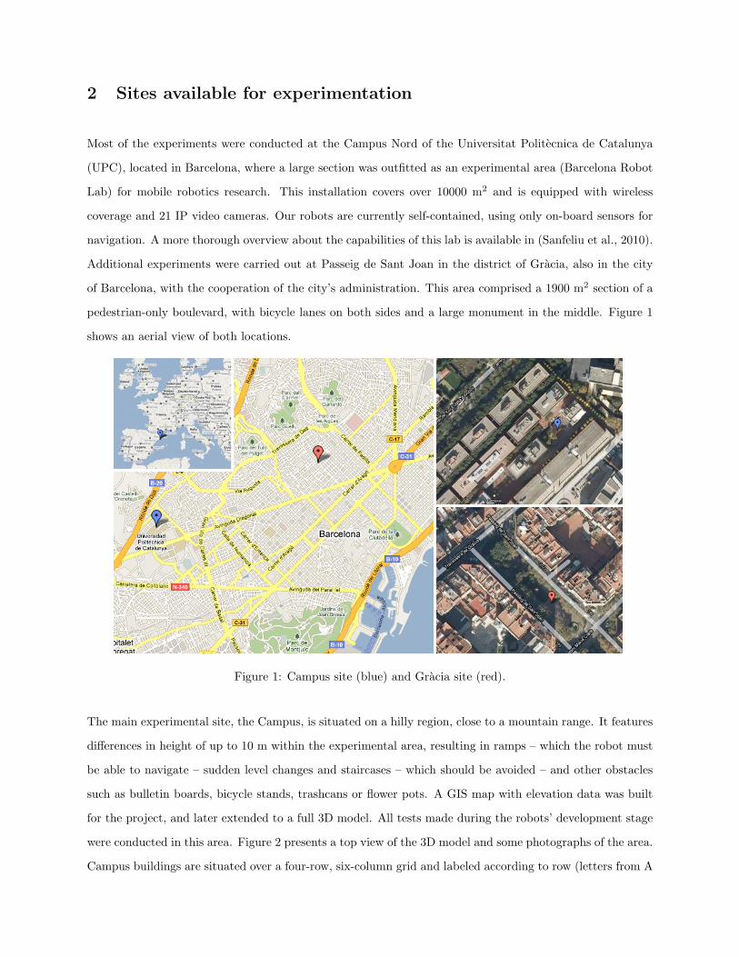
Additional experiments were carried out at Passeig de Sant Joan in the district of Gracia, also in the city
of Barcelona, with the cooperation of the city’s administration. This area comprised a 1900 m2 section of a
pedestrian-only boulevard, with bicycle lanes on both sides and a large monument in the middle. Figure 1
shows an aerial view of both locations.
Figure 1: Campus site (blue) and Gracia site (red).
The main experimental site, the Campus, is situated on a hilly region, close to a mountain range. It features
differences in height of up to 10 m within the experimental area, resulting in ramps – which the robot must
be able to navigate – sudden level changes and staircases – which should be avoided – and other obstacles
such as bulletin boards, bicycle stands, trashcans or flower pots. A GIS map with elevation data was built
for the project, and later extended to a full 3D model. All tests made during the robots’ development stage
were conducted in this area. Figure 2 presents a top view of the 3D model and some photographs of the area.
Campus buildings are situated over a four-row, six-column grid and labeled according to row (letters from A

to D, bottom to top) and column (numbers from 1 to 6, left to right), e.g. A1 or D6. The experimental area
covers the eastern part of the campus. The main features found on this area are the terrace at the bottom
of the map, the FIB (Computer Faculty) square and cafeteria, and a promenade with another terrace above
it, between rows B and C.
The site at Passeig de Sant Joan does not feature ramps or staircases, but is again on sloped terrain, rising
more than 2 m in height along 70 m of length, with a relatively even slope of nearly 2◦. This poses a problem
for two-wheeled robots such as ours, as will be further explained in section 3. It is of particular interest that
there are few clear landmarks such as walls, as most of the area is encircled by hedges on either side, and the
monument in the middle was at the time (spring) surrounded by rose bushes. While the campus scenario
is somewhat controlled and mostly populated by students, the Gracia environment is a very crowded public
street in the middle of a large city, frequented by pedestrians, children and bicyclists. A 3D model of the
area was built from scratch, in much lesser detail. The area is pictured in figure 3. We placed four fences
below the monument for safety reasons, which were included in the 3D map. Later on we had to put other
fences in place to reroute part of the traffic, but these were not included in the map.
3 Robots
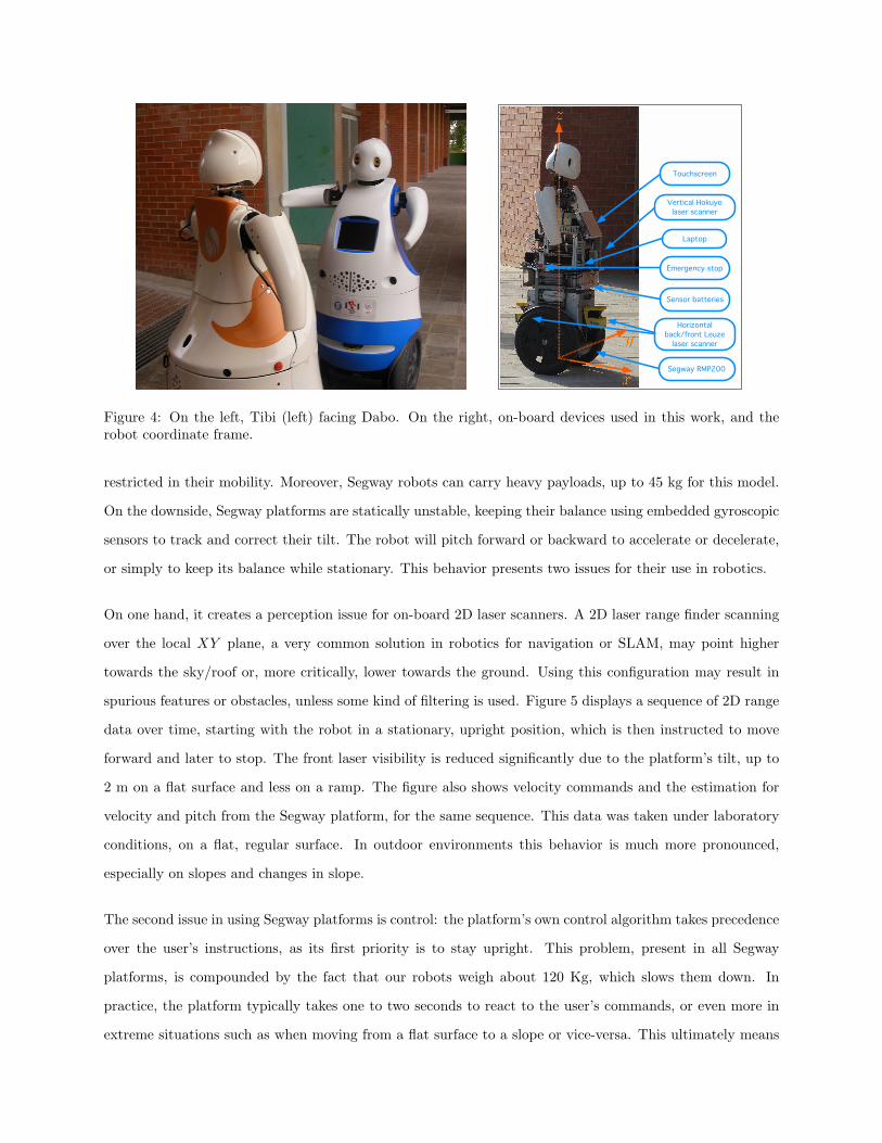
Two mobile service robots, designed to operate in urban, pedestrian areas, were developed for the URUS
project. These are Tibi and Dabo, pictured in figure 4. They are based on two-wheeled, self-balancing
Segway RMP200 platforms, and as such are highly mobile, with a small footprint, a nominal speed up to
4.4 m/s, and the ability to rotate on the spot (while stationary).
They are equipped with the following sensors:
• Two Leuze RS4 2D laser range finders, scanning over the local XY plane, pointing forward and
backward respectively, at a height of 40 cm from the ground. These scanners provide 133 points
over 190◦ at the fastest setting, running at approximately 6 Hz. This device has a range of 64 m,
but in practice we use a 15 m cap. Front and back laser observations are notated as otLF and otLB
respectively.
• A third 2D laser scanner, a Hokuyo UTM-30LX, mounted at a height of 90 cm., pointing forward
and rotated 90◦ over its side, scanning over the local XZ plane. This scanner provides 1081 points
over 270◦ at 40 Hz, and has a range of 30 m, again capped to 15 m. Aperture is limited to 60◦ to
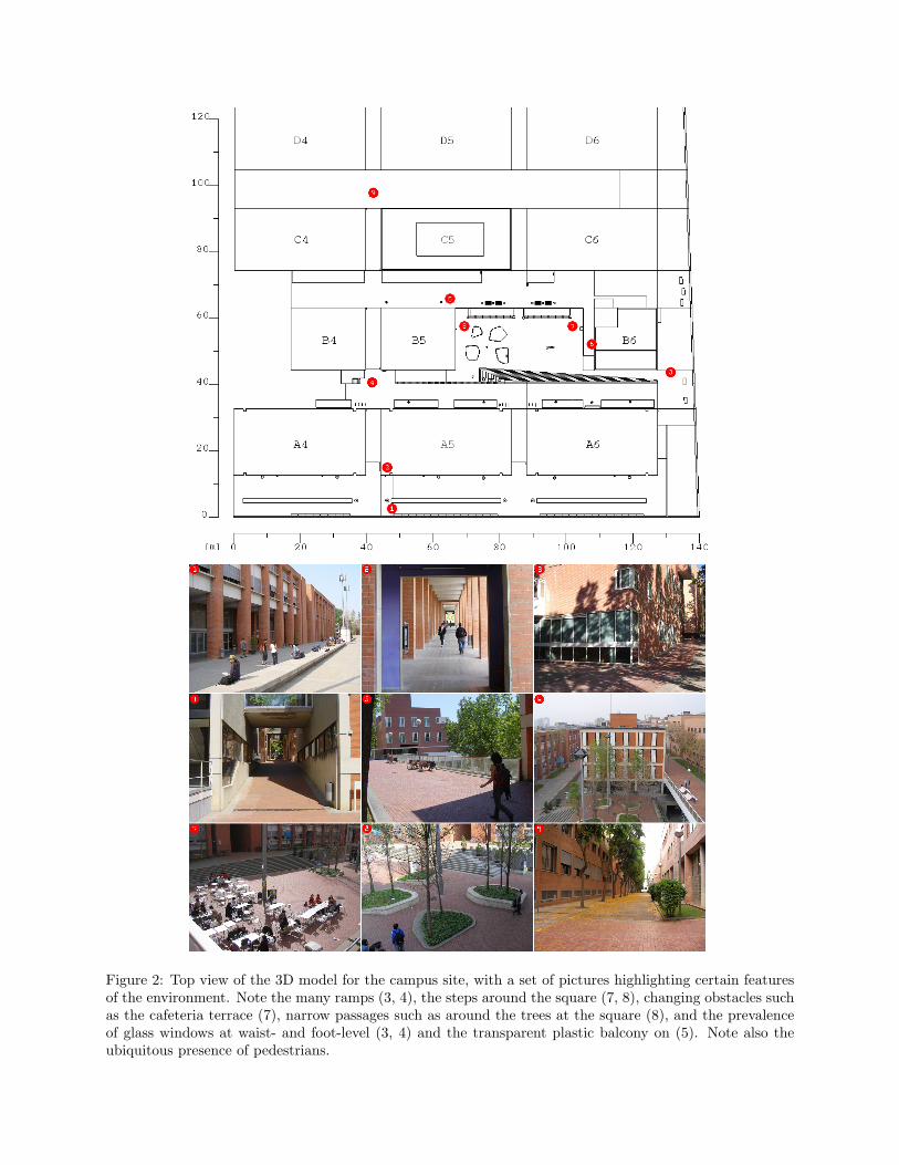
Figure 2: Top view of the 3D model for the campus site, with a set of pictures highlighting certain featuresof the environment. Note the many ramps (3, 4), the steps around the square (7, 8), changing obstacles suchas the cafeteria terrace (7), narrow passages such as around the trees at the square (8), and the prevalenceof glass windows at waist- and foot-level (3, 4) and the transparent plastic balcony on (5). Note also theubiquitous presence of pedestrians.
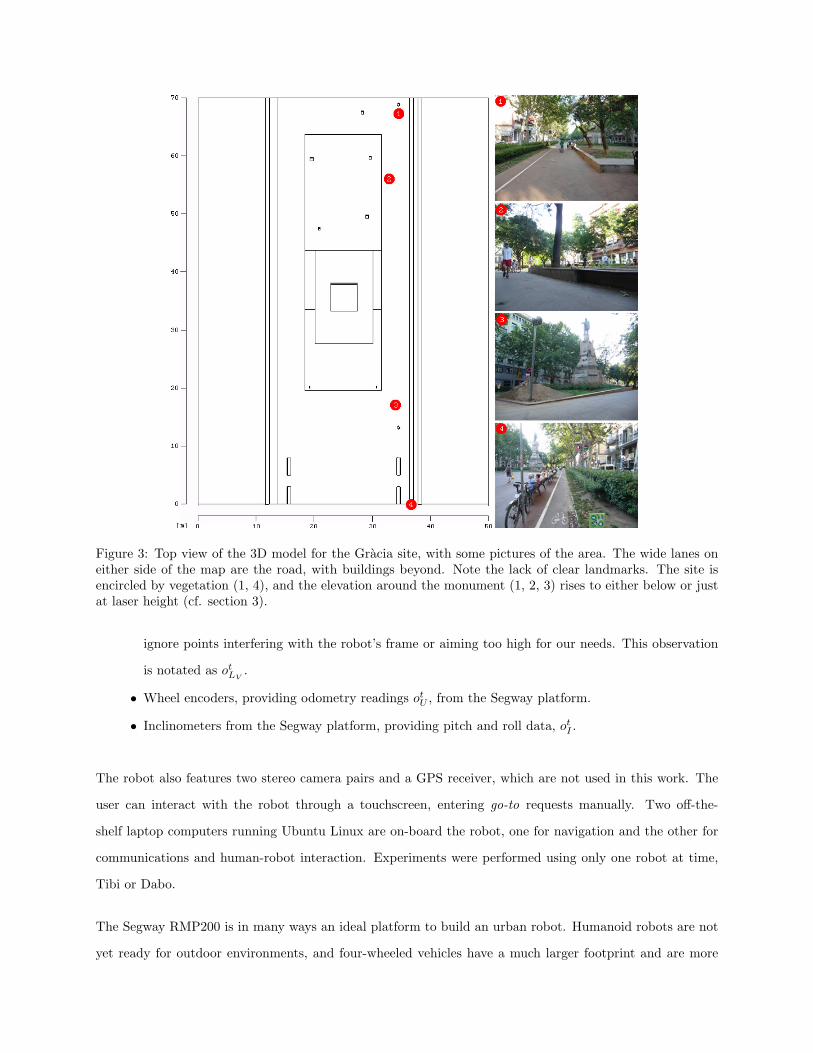
Figure 3: Top view of the 3D model for the Gracia site, with some pictures of the area. The wide lanes oneither side of the map are the road, with buildings beyond. Note the lack of clear landmarks. The site isencircled by vegetation (1, 4), and the elevation around the monument (1, 2, 3) rises to either below or justat laser height (cf. section 3).
ignore points interfering with the robot’s frame or aiming too high for our needs. This observation
is notated as otLV .
• Wheel encoders, providing odometry readings otU , from the Segway platform.
• Inclinometers from the Segway platform, providing pitch and roll data, otI .
The robot also features two stereo camera pairs and a GPS receiver, which are not used in this work. The
user can interact with the robot through a touchscreen, entering go-to requests manually. Two off-the-
shelf laptop computers running Ubuntu Linux are on-board the robot, one for navigation and the other for
communications and human-robot interaction. Experiments were performed using only one robot at time,
Tibi or Dabo.
The Segway RMP200 is in many ways an ideal platform to build an urban robot. Humanoid robots are not
yet ready for outdoor environments, and four-wheeled vehicles have a much larger footprint and are more
Touchscreen
Vertical Hokuyo
laser scanner
Laptop
Emergency stop
Sensor batteries
Horizontal
back/front Leuze
laser scanner
Segway RMP200
Figure 4: On the left, Tibi (left) facing Dabo. On the right, on-board devices used in this work, and therobot coordinate frame.
restricted in their mobility. Moreover, Segway robots can carry heavy payloads, up to 45 kg for this model.
On the downside, Segway platforms are statically unstable, keeping their balance using embedded gyroscopic
sensors to track and correct their tilt. The robot will pitch forward or backward to accelerate or decelerate,
or simply to keep its balance while stationary. This behavior presents two issues for their use in robotics.
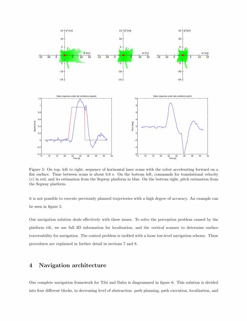
On one hand, it creates a perception issue for on-board 2D laser scanners. A 2D laser range finder scanning
over the local XY plane, a very common solution in robotics for navigation or SLAM, may point higher
towards the sky/roof or, more critically, lower towards the ground. Using this configuration may result in
spurious features or obstacles, unless some kind of filtering is used. Figure 5 displays a sequence of 2D range
data over time, starting with the robot in a stationary, upright position, which is then instructed to move
forward and later to stop. The front laser visibility is reduced significantly due to the platform’s tilt, up to
2 m on a flat surface and less on a ramp. The figure also shows velocity commands and the estimation for
velocity and pitch from the Segway platform, for the same sequence. This data was taken under laboratory
conditions, on a flat, regular surface. In outdoor environments this behavior is much more pronounced,
especially on slopes and changes in slope.
The second issue in using Segway platforms is control: the platform’s own control algorithm takes precedence
over the user’s instructions, as its first priority is to stay upright. This problem, present in all Segway
platforms, is compounded by the fact that our robots weigh about 120 Kg, which slows them down. In
practice, the platform typically takes one to two seconds to react to the user’s commands, or even more in
extreme situations such as when moving from a flat surface to a slope or vice-versa. This ultimately means
14 16 18 20 22 24 26 28 30 32−0.4
−0.2
0
0.2
0.4
0.6
0.8
1
1.2
Time [s]
Speed [m
/s]
Dabo response under lab conditions (speed)
14 16 18 20 22 24 26 28 30 32−6
−4
−2
0
2
4
6
8
10
Time [s]
Pitch [deg]
Dabo response under lab conditions (pitch)
Figure 5: On top, left to right, sequence of horizontal laser scans with the robot accelerating forward on aflat surface. Time between scans is about 0.6 s. On the bottom left, commands for translational velocity(v) in red, and its estimation from the Segway platform in blue. On the bottom right, pitch estimation fromthe Segway platform.
it is not possible to execute previously planned trajectories with a high degree of accuracy. An example can
be seen in figure 5.
Our navigation solution deals effectively with these issues. To solve the perception problem caused by the
platform tilt, we use full 3D information for localization, and the vertical scanner to determine surface
traversability for navigation. The control problem is tackled with a loose low-level navigation scheme. These
procedures are explained in further detail in sections 7 and 8.
4 Navigation architecture
Our complete navigation framework for Tibi and Dabo is diagrammed in figure 6. This solution is divided
into four different blocks, in decreasing level of abstraction: path planning, path execution, localization, and
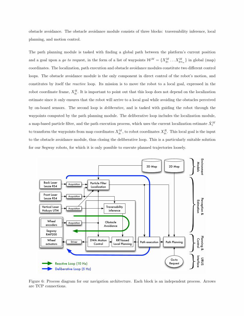
obstacle avoidance. The obstacle avoidance module consists of three blocks: traversability inference, local
planning, and motion control.
The path planning module is tasked with finding a global path between the platform’s current position
and a goal upon a go to request, in the form of a list of waypoints WM = {XMg1 . . . X
MgNw} in global (map)
coordinates. The localization, path execution and obstacle avoidance modules constitute two different control
loops. The obstacle avoidance module is the only component in direct control of the robot’s motion, and
constitutes by itself the reactive loop. Its mission is to move the robot to a local goal, expressed in the
robot coordinate frame, XRgi . It is important to point out that this loop does not depend on the localization
estimate since it only ensures that the robot will arrive to a local goal while avoiding the obstacles perceived
by on-board sensors. The second loop is deliberative, and is tasked with guiding the robot through the
waypoints computed by the path planning module. The deliberative loop includes the localization module,
a map-based particle filter, and the path execution process, which uses the current localization estimate XMr
to transform the waypoints from map coordinates XMgi , to robot coordinates XR
gi . This local goal is the input
to the obstacle avoidance module, thus closing the deliberative loop. This is a particularly suitable solution
for our Segway robots, for which it is only possible to execute planned trajectories loosely.
ObstacleAvoidance
Segway RMP200
Back LaserLeuze RS4
Acquisition Particle Filter Localization
Front LaserLeuze RS4
Acquisition
Vertical LaserHokuyo UTM
Acquisition
Wheel encoders
Acquisition
Driver
Traversability inference
DWA Motion Control
RRT-based Local Planning
Path Planning
3D Map 2D Map
Wheel actuators
Reactive Loop (10 Hz)
Deliberative Loop (5 Hz)
Go-to
Request
Perce
ptio
n &
Estim
atio
nPla
nning &
Contro
lURUS
Interfa
ce
Path execution
Enviro
nment
Models
Figure 6: Process diagram for our navigation architecture. Each block is an independent process. Arrowsare TCP connections.
We use two different environment models, a 2D map and a 3D map. The 3D map is a model containing
the environment’s static geometry. The 2D map is inherited from previous work (Corominas Murtra et al.,
2010b) and is required for path planning. The reactive loop runs at 10 Hz and the deliberative loop runs at
5 Hz. Since the platform moves at speeds up to 1 m/s these rates are deemed sufficient.
Each sensor has an associated data acquisition process. All navigation and data acquisition processes run
concurrently in the same computer. The software framework follows a publish/subscriber architecture, with
the aim to ease software integration between developers: each block of figure 6 has been implemented
as an independent process, accessible through an interface. The resulting specification runs over YARP
as middleware, a free, open-source, platform-independent set of libraries, protocols and tools aimed at
decoupling the transmission of information from the particulars of devices and processes in robotic systems
(Metta et al., 2006). For a further description of our software architecture, please refer to (Corominas Murtra
et al., 2008).
5 Path planning
Our planning algorithm has been developed in the context of the URUS project, having as a key requirement
the ability to effectively deal with the diversity of platforms involved in the project. Thus, we have privileged
reliability and flexibility over other concerns such as on-line replanning. That said, it is worth noting that
limited on-line planning capabilities are actually fulfilled by the local planning component of our architecture
(cf. 8.1).
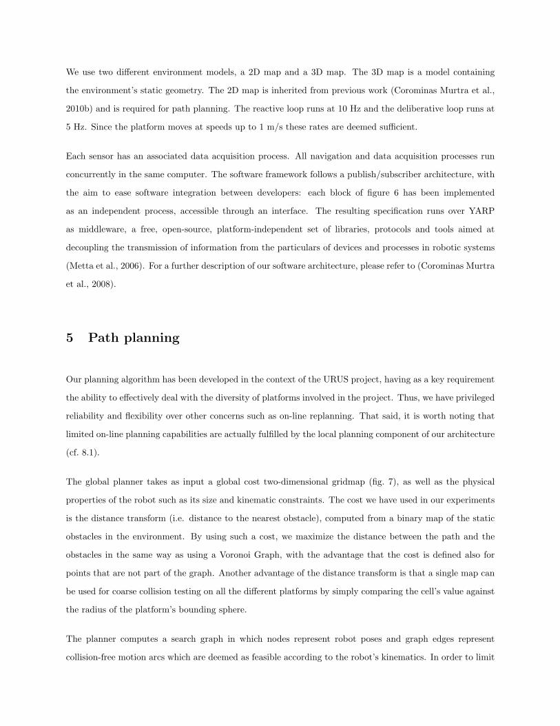
The global planner takes as input a global cost two-dimensional gridmap (fig. 7), as well as the physical
properties of the robot such as its size and kinematic constraints. The cost we have used in our experiments
is the distance transform (i.e. distance to the nearest obstacle), computed from a binary map of the static
obstacles in the environment. By using such a cost, we maximize the distance between the path and the
obstacles in the same way as using a Voronoi Graph, with the advantage that the cost is defined also for
points that are not part of the graph. Another advantage of the distance transform is that a single map can
be used for coarse collision testing on all the different platforms by simply comparing the cell’s value against
the radius of the platform’s bounding sphere.
The planner computes a search graph in which nodes represent robot poses and graph edges represent
collision-free motion arcs which are deemed as feasible according to the robot’s kinematics. In order to limit
Figure 7: On the left, the cost map for the UPC campus. Warmer tones indicate high costs, white indicatesunreachable places. On the right, three sample paths displayed using our simulation environment. Red dotsindicate the path computed by the path planning module. Red circles correspond to the circle path, whichwill be introduced in the following section. Green and blue dots correspond to the localization estimate andmark the starting position for each iteration. Further examples are available in the videos introduced insection 9.
the size of the search space, graph expansion is performed using a fixed arc-length and a discrete number of
arc curvatures. The graph is explored using the A∗ algorithm, where the heuristic is the naıve grid-distance
to the goal, computed on the cost map using Dijkstra’s algorithm.
It is worth noting that using a fixed arc length and angle discretization implies, in most cases, that the plan
is not able to reach the exact goal pose making it necessary to use an acceptance threshold. However, in
practice this has not been a problem. We have used a threshold of 30 cm, which is precise enough for our
particular application.
As stated above, this module was common to all robotic platforms in the project. Our navigation system
defers on-line replanning to the obstacle avoidance module, and has simpler requirements for global path
planning: the distance between waypoints is set to 2 m for Tibi and Dabo, and we disregard heading angle
data for the waypoint. Examples of its application are displayed in figure 7.
6 Path execution
The task of the path execution algorithm is to provide local goal points to the robot so that the trajectory
computed by the global planner is followed in a smooth manner, even with the presence of unmapped

obstacles that force the robot to stray out of the path. Our approach consists in defining circle-based search
zones centered on the plan’s waypoints. The localization estimate is then used to determine which circle the
robot lies on, if any, and the next waypoint to target, which is then transformed into robot coordinates and
sent to the obstacle avoidance module as a local goal.
The circle path is created upon receiving a new path from the global planner, once per go to request, and is
defined as a list of circles {C1 . . . CNw} with center each waypoint and radius the distance to the following
waypoint. The radius for the last circle, with center the goal, is defined as the goal tolerance dg, a global
parameter set to 0.5 m. The algorithm stores an index to the circle currently being followed, k, which is
initialized to 2, as XMg1 is the robot’s starting position. During runtime, the algorithm determines whether
the circle currently being followed and its adjacent circles Ck−1, Ck+1 contain the localization estimate XMr ,
starting from the higher index and moving down. Whenever this is true the process stops and k is set to the
index of the compliant circle. The waypoint to target is in every case the center of the next circle, Ck+1,
which by definition lies on the circumference of Ck. That is, when a robot nears a waypoint (enters its
associated circle), the goal will switch to the next waypoint (the center of the next circle). We check only
the next circle to enforce smoothness, and the previous circle as a safeguard against small variations on the
localization estimate. This procedure is illustrated in figure 8.
Figure 8: Illustration demonstrating the behavior of the path execution algorithm under normal operatingconditions. Waypoints and the circle path are plotted in red when considered by the path execution algorithm,in purple when not. The localization estimate and an arrow signaling the current target are plotted in green.The environment (unbeknown to the path execution module) is plotted in black. On the left, the circlecurrently being followed is CN−2, centered on waypoint XM
N−2, and so the current target is XMN−1. The
algorithm considers this circle and its neighbors, in this order: first CN−1, then CN−2 and finally CN−3. Asthe first circle that contains the localization estimate is CN−2, the target does not change. On the right, therobot moves forward and enters circle CN−1, so that the new circle being followed is CN−1 and XM
N becomesthe new target.
If no circle contains the localization estimate we compute its distance to the path, defined as the shortest

distance to a waypoint. If this distance is smaller than the recovery distance dr, set to 3 m, the path
execution algorithm will enter recovery mode, sending the robot to the closest waypoint. When the robot is
farther away than the recovery distance we presume recovery is not possible, stop the robot, and request the
path planning module for a new path to the same global goal. These situations are illustrated in figure 9.
Figure 7 displays examples of circle paths in the campus area.
Figure 9: Illustration demonstrating the behavior of the path execution module when the robot strays offthe path. The dashed circles determine the recovery zone. On the left, the robot is following circle CN−2,targeting waypoint XM
N−1, but moves off the circle path and is instructed to return to XN−2. On the right,the robot strays farther off the path and moves out of the recovery zone, prompting the algorithm to stopthe robot and request a new path from the global planner, plotted in blue. The old path is discarded.
This approach is valid for obstacle-free environments, but may fail if an unmapped object rests over a
waypoint which thus cannot be reached. We solve this by computing not one but an array of goal candidates
GR, which are offered to the obstacle avoidance module as possible targets. Being XMj the current target,
we consider all waypoints {XMi |i ∈ [j,Nw]}. We take a maximum of NOA points, and only candidates closer
to the robot than dOA are considered valid. The first candidate that violates this rule is truncated to dOA
and the rest are ignored. For our implementation we use dOA = 5.5 m, and NOA = 8. This guarantees at
least three goal candidates within range. The obstacle avoidance module considers one candidate at a time,
starting from the lower index, and selects the first candidate that may be reached, as explained in section 8.
7 Map-based localization
Localization is the process in charge of closing the deliberative loop (fig. 6), thus allowing the path execution
module to convert goal points from the global planner, in map coordinates, to local goal points, in robot
coordinates. Localization plays a key role in autonomous navigation for mobile robots and a vast amount
of work can be found in the literature. It is accepted by mobile robot researchers that GPS-based solutions
are not robust enough in urban environments due to insufficient accuracy and partial coverage. This fact
has forced the mobile robotics community to design alternative or complementary methods for localization
(Thrun et al., 2001; Georgiev and Allen, 2004; Levinson et al., 2007; Yun and Miura, 2007; Nuske et al.,
2009).
In recent years, researchers worldwide have opted for particle filter-based solutions for localization (Thrun
et al., 2001; Levinson et al., 2007; Nuske et al., 2009), which offer design advantages and greater flexibility
than approaches based on the Kalman Filter (Arras et al., 2003; Georgiev and Allen, 2004; Yun and Miura,
2007). However, when particle filter localization is developed for autonomous navigation, it has to deal
with real-time requirements. Particle filters need to compute expected observations from particle positions.
Computations can be performed off-line and then stored in large look-up tables discretizing the space of
positions, so that during on-line executions these look-up tables will be queried from particle positions
(Thrun et al., 2001; Levinson et al., 2007). However, when the robot operates in large environments and the
position space has a dimensionality greater than 3, precomputing expected observations becomes a critical
database issue.
In this section we describe a 3D map-based localization method, consisting of a particle filter that computes
the expected observations on-line by means of fast manipulation of a 3D geometric model of the environment,
implemented using the OpenGL library (OpenGL website, ). Using OpenGL for on-line observation model
computations has already been proposed by some researchers (Nuske et al., 2009). However, in that paper
the authors use an edge map of the environment and compute only expected edge observations. Our approach
does not perform any feature extraction step and deals with on-line computation of the full sensor model, so
that real sensor data is directly compared with expected sensor data to score the particles in the filter loop.
This approach overcomes the issue of feature occlusion due to the ubiquitous presence of pedestrians and
other unmodeled obstacles around the robot, achieving robust tracking of the robot’s position. Our solution
runs at 5 Hz, enough for our platform’s speed.
7.1 State Space
The state space considered in our approach, X, is that of 3D positions, parametrized as a (x, y, z) location
referenced to the map frame, and the three Euler angles, heading, pitch and roll, (θ, φ, ψ), defined starting
with the heading angle with respect to the x map axis. In this section, all positions will be referenced to the
map frame if no specific mark or comment indicates otherwise.
At each iteration t, the filter produces a set of particles, P t, where each particle is a pair formed by a position
in the state space and a weight:
P t = {st1 . . . stNP }; sti = (Xt
i , wti); X
ti = (xti, y
ti , z
ti , θ
ti , φ
ti, ψ
ti) (1)
where sti is the ith particle produced by the tth iteration, Xti ∈ X, and wti ∈ [0, 1].
7.2 3D environment model
The environment model used by the localization module, also referred to as the map, and notated asM, is a
geometric 3D representation of the static part of the area where the robot operates. In both the Campus and
Gracia areas, the static part considered includes buildings, stairs, ramps, borders, curbs, some important
vegetation elements and urban furniture such as benches or streetlamps. Our implementation uses the .obj
geometry definition file format (OBJ file format, ), originally developed for 3D computer animation and
scene description, which has become an open format and a de facto exchange standard.
Both maps were built by hand, taking measurements with laser distance meters and measuring tape, which
were used to build a coherent 3D model. Even if the maps incorporate the most important geometrical
elements of each experimental area, they are always considered incomplete models: for instance, trees were
only modeled partially, due to the difficulty of doing so, and minor urban furniture was not always mapped.
Thus, the localization approach should be robust enough to address this issue. Further details are available
in (Corominas Murtra et al., 2010a).
7.3 Kinematic model
In particle filtering, having a motion model allows to propagate the particle set, thus limiting the search
space to positions satisfying the motion model constrained to given sensor inputs. Probabilistic kinematic
models (Thrun et al., 2005) compute a new sample set, called the prior, P t−
, based on the previous set,
P t−1, constrained to the platform’s motion. We define the platform wheel odometry readings as:
otU = (∆tρ,∆
tθ) (2)
where ∆tρ is the translational 2D increment in the local XY plane, and ∆t
θ is the rotational increment around
the local Z axis of the platform. Both increments are the accumulated odometry from iteration t − 1 up
to iteration t. The Segway RMP200 platform also features embedded inclinometers that provide a pitch
increment measure from t− 1 to t:
otI = ∆tφ (3)
With these two input observations, at the beginning of each iteration, the state of the ith particle is moved
according the probabilistic kinematic model described by:
∆tρ,i = N (∆t
ρ, σtρ); σ
tρ = ερ∆t
ρ
∆tθ,i = N (∆t
θ, σtθ); σ
tθ = εθ∆t
θ
∆tφ,i = N (∆t
φ, σtφ); σtφ = εφ∆t
φ
xti = xt−1i + ∆t
ρ,i cos
(θt−1i +
∆tθ,i
2
)
yti = yt−1i + ∆t
ρ,i sin
(θt−1i +
∆tθ,i
2
)
θti = θt−1i + ∆t
θ,i
φti = φt−1i + ∆t
φ,i
(4)
where the first three lines draw, for each particle, random data with normal distribution centered at the
platform data (∆tρ,∆
tθ,∆
tφ) with standard deviation depending linearly with each respective increment by
parameters ερ, εθ, εφ, so that large increments imply a more sparse propagation. Epsilon values were set to
ε{ρ,θ,φ} = 0.2 during the experimental sessions.
Please note that the orientation angles of a Segway robot do not necessarily indicate a displacement direction
since the platform is unconstrained in pitch. Thus, this kinematic model approximates displacements in the
local plane provided by the platform odometry as displacements in the global (map) XY plane. This
approximation leads to an error that is negligible in practice since the slopes in our test environments have
at most an inclination of 10%. Note also that the kinematic model does not modify zti and ψti since these
two variables are constrained by gravity, as will be explained in the next subsection.
7.4 Gravity Constraints
A wheeled robot will always lie on the floor, due to gravity. For relatively slow platforms, as those presented
in section 3, it can be assumed as well that the whole platform is a rigid body, so that a suspension system,
if present, does not modify the attitude of the vehicle. With these assumptions, and for two-wheeled self-
balancing platforms, there are constraints on the height z and roll ψ dimensions of the position space, given
a (x, y, θ) triplet and the environment model M. Both constraints will be computed using OpenGL for fast
manipulation of 3D models.
The height constraint sets a height, z, for a given coordinate pair (x, y). To compute it, the floor part of
the map is rendered in a small window (5×5 pixels) from an overhead viewpoint at (x, y, zoh), limiting the
projection to a narrow aperture (1◦). After rendering we obtain the depth component of the central pixel,
dc, and compute the constrained z value as z = zoh − dc.
The roll constraint fixes the roll component, for a coordinate triplet (x, y, θ). Its computation is based on
finding zr and zl, the height constraints at two points to the left and to the right of (x, y, θ). These points
are separated a known distance L (i.e. size of the platform), so that the roll constraint can be computed as
ψ = atan2(zl − zr, L).
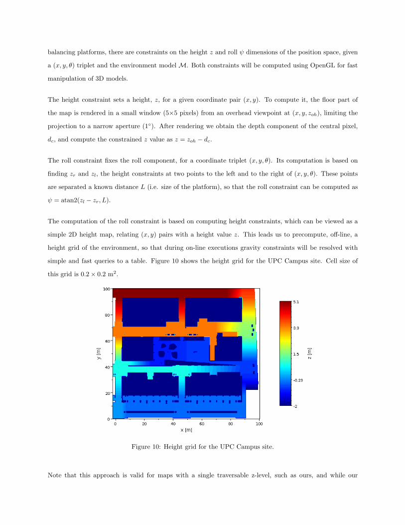
The computation of the roll constraint is based on computing height constraints, which can be viewed as a
simple 2D height map, relating (x, y) pairs with a height value z. This leads us to precompute, off-line, a
height grid of the environment, so that during on-line executions gravity constraints will be resolved with
simple and fast queries to a table. Figure 10 shows the height grid for the UPC Campus site. Cell size of
this grid is 0.2× 0.2 m2.
Figure 10: Height grid for the UPC Campus site.
Note that this approach is valid for maps with a single traversable z-level, such as ours, and while our
algorithms can be directly applied to multi-level maps further work would be required in determining the
appropriate map section to compute. To avoid discretization problems, specially when computing the roll
constraint using the height grid, we use lineal interpolation on the grid.
7.5 Range Observation Model & Similarity Metrics
Fast and accurate computation of observation models is a key issue for successful particle filtering. The
result of computing an observation model is an expected observation computed from a particle position,
denoted as osL(Xti ) for a laser scanner. Given this expected observation, the conditional probability of an
actual laser observation given that the robot is in particle position Xti can be approximated as:
p(otL|Xti ) ∼ L(otL, o
sL(Xt
i )), ∈ [0, 1] (5)
where L is a similarity function measuring the closeness of two laser observations. This subsection first
details how the expected observations osL are computed and then presents the similarity function used to
compare real and expected laser scanner data.
We propose a method using the OpenGL library for fast on-line computation of expected laser scanner
observations. The method is based on rendering the 3D model from the viewpoint of the sensor’s position
given the particle position Xti , and reading the depth buffer of the computer graphics card. The rendering
window size has been minimized to reduce the computation time while keeping the sensor’s accuracy given
by the scanner aperture, ∆α, and the number of scan points NL. Algorithm 1 outlines the procedure to
compute an expected laser scan from a particle position Xti , given a 3D environment model M and a set of
sensor parameters (∆α, NL, rmin, rmax), being respectively: the angular scan aperture, the number of scan
points, and range limits.
Since the Leuze scanner has an aperture greater than 180◦, we divide the computation in two sectors. For
the Hokuyo scanner we use only an aperture of 60◦, so that a single sector is enough. According to the
device parameters detailed on section 3, the resulting window sizes are 88×5 pixels for the Leuze device (for
each sector) and 265×5 pixels for the Hokuyo scanner. This optimized implementation allows the filter to
run at 5 Hz while computing at each iteration NP × (133 + 133 + 241) ranges. For NP = 50 particles, this
implies 126750 ranges per second. Further details on computing such expected range observations can be
found at (Corominas Murtra et al., 2010a).
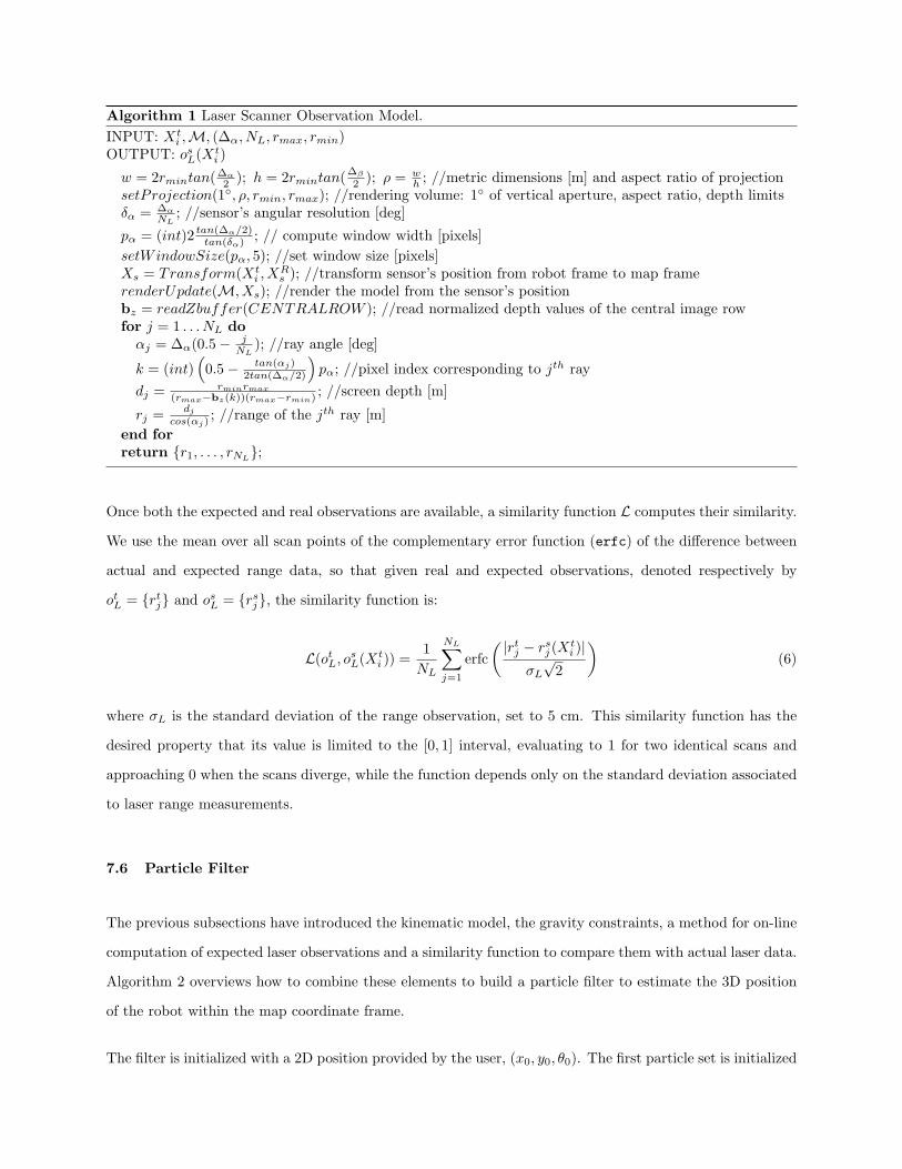
Algorithm 1 Laser Scanner Observation Model.INPUT: Xt
i ,M, (∆α, NL, rmax, rmin)OUTPUT: osL(Xt
i )
w = 2rmintan(∆α
2 ); h = 2rmintan(∆β
2 ); ρ = wh ; //metric dimensions [m] and aspect ratio of projection
setProjection(1◦, ρ, rmin, rmax); //rendering volume: 1◦ of vertical aperture, aspect ratio, depth limitsδα = ∆α
NL; //sensor’s angular resolution [deg]
pα = (int)2 tan(∆α/2)tan(δα) ; // compute window width [pixels]
setWindowSize(pα, 5); //set window size [pixels]Xs = Transform(Xt
i , XRs ); //transform sensor’s position from robot frame to map frame
renderUpdate(M, Xs); //render the model from the sensor’s positionbz = readZbuffer(CENTRALROW ); //read normalized depth values of the central image rowfor j = 1 . . . NL doαj = ∆α(0.5− j
NL); //ray angle [deg]
k = (int)(
0.5− tan(αj)2tan(∆α/2)
)pα; //pixel index corresponding to jth ray
dj = rminrmax(rmax−bz(k))(rmax−rmin) ; //screen depth [m]
rj = djcos(αj)
; //range of the jth ray [m]end forreturn {r1, . . . , rNL};
Once both the expected and real observations are available, a similarity function L computes their similarity.
We use the mean over all scan points of the complementary error function (erfc) of the difference between
actual and expected range data, so that given real and expected observations, denoted respectively by
otL = {rtj} and osL = {rsj}, the similarity function is:
L(otL, osL(Xt
i )) =1NL
NL∑j=1
erfc( |rtj − rsj (Xt
i )|σL√
2
)(6)
where σL is the standard deviation of the range observation, set to 5 cm. This similarity function has the
desired property that its value is limited to the [0, 1] interval, evaluating to 1 for two identical scans and
approaching 0 when the scans diverge, while the function depends only on the standard deviation associated
to laser range measurements.
7.6 Particle Filter
The previous subsections have introduced the kinematic model, the gravity constraints, a method for on-line
computation of expected laser observations and a similarity function to compare them with actual laser data.
Algorithm 2 overviews how to combine these elements to build a particle filter to estimate the 3D position
of the robot within the map coordinate frame.
The filter is initialized with a 2D position provided by the user, (x0, y0, θ0). The first particle set is initialized
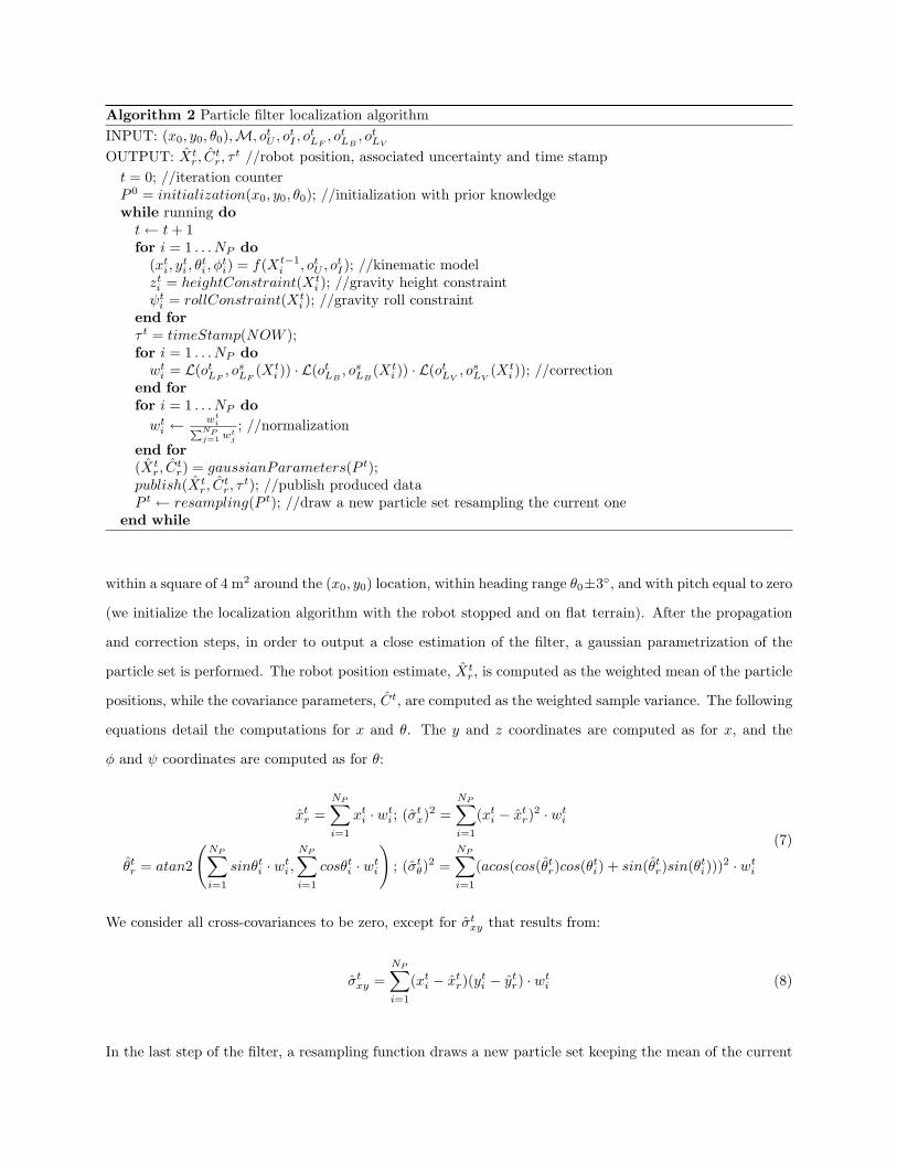
Algorithm 2 Particle filter localization algorithmINPUT: (x0, y0, θ0),M, otU , o
tI , o
tLF, otLB , o
tLV
OUTPUT: Xtr, C
tr, τ
t //robot position, associated uncertainty and time stampt = 0; //iteration counterP 0 = initialization(x0, y0, θ0); //initialization with prior knowledgewhile running dot← t+ 1for i = 1 . . . NP do
(xti, yti , θ
ti , φ
ti) = f(Xt−1
i , otU , otI); //kinematic model
zti = heightConstraint(Xti ); //gravity height constraint
ψti = rollConstraint(Xti ); //gravity roll constraint
end forτ t = timeStamp(NOW );for i = 1 . . . NP dowti = L(otLF , o
sLF
(Xti )) · L(otLB , o
sLB
(Xti )) · L(otLV , o
sLV
(Xti )); //correction
end forfor i = 1 . . . NP dowti ←
wtiPNPj=1 w
tj
; //normalization
end for(Xt
r, Ctr) = gaussianParameters(P t);
publish(Xtr, C
tr, τ
t); //publish produced dataP t ← resampling(P t); //draw a new particle set resampling the current one
end while
within a square of 4 m2 around the (x0, y0) location, within heading range θ0±3◦, and with pitch equal to zero
(we initialize the localization algorithm with the robot stopped and on flat terrain). After the propagation
and correction steps, in order to output a close estimation of the filter, a gaussian parametrization of the
particle set is performed. The robot position estimate, Xtr, is computed as the weighted mean of the particle
positions, while the covariance parameters, Ct, are computed as the weighted sample variance. The following
equations detail the computations for x and θ. The y and z coordinates are computed as for x, and the
φ and ψ coordinates are computed as for θ:
xtr =NP∑i=1
xti · wti ; (σtx)2 =NP∑i=1
(xti − xtr)2 · wti
θtr = atan2
(NP∑i=1
sinθti · wti ,NP∑i=1
cosθti · wti
); (σtθ)
2 =NP∑i=1
(acos(cos(θtr)cos(θti) + sin(θtr)sin(θti)))
2 · wti
(7)
We consider all cross-covariances to be zero, except for σtxy that results from:
σtxy =NP∑i=1
(xti − xtr)(yti − ytr) · wti (8)
In the last step of the filter, a resampling function draws a new particle set keeping the mean of the current

one. Resampling is necessary to avoid particle depletion (Doucet et al., 2001; Arulampalam et al., 2002),
an undesired phenomenon of particle filters where the particle set collapses to a single state point rendering
the filter no longer capable of exploring new solutions for the estimation, and therefore compromising its
robustness.
As an aside, the vertical laser is integrated into the correction stage only when appropriate. Most unmodeled
obstacles, such as pedestrians or bicyclists, have a relatively small footprint on the XY plane, so that the
horizontal lasers remain usable despite numerous occlusions (as our experiments demonstrate). The vertical
scanner on the other hand can be nearly fully occluded by a single pedestrian a few meters in front of the
robot. In that scenario the filter attempts to match actual and expected observations by pitching the robot
forward, lifting the floor surface towards the part of the scan corresponding to the pedestrian, and thus
increasing the similarity between scans. This is clearly inadequate and compromises the filter’s performance,
so we use the vertical laser only when the difference between actual and expected observations, as computed
by the similarity function, is smaller than a threshold, determined experimentally. We do not want to
perform feature extraction or segmentation over the raw scan, but there exist more elaborate solutions, such
as iteratively considering sets of data removing the points further away from the robot until the threshold
is met. These shall be explored in the future.
Section 9 summarizes the field work and discusses in depth the two failures we experienced during the
experiments, both due to localization issues.
8 Obstacle avoidance
The motion planning problem is well known and studied when using a priori information (Latombe, 1991).
However, many techniques are not applicable when the environment is not known or highly dynamic. This
problem is compounded by the fact that both the environment (i.e. the real world) and the robot carry
uncertainties due to sensing and actuation, respectively, so that it is not feasible to treat motion planning
separately from its execution. To solve these problems it is necessary to incorporate sensory information
in the planning and control loop, making possible reactive navigation. A real-time approach based on
the artificial potential field concept was presented in (Khatib, 1986), was later extended in (Khatib and
Chatila, 1995) and became widely used, as for instance in (Haddad et al., 1998). Other methods extract
higher-level information from the sensor data, such as for instance (Minguez and Montano, 2004), a reactive
obstacle avoidance system for complex, cluttered environments based on inferring regions from geometrical

properties. None of these methods take into account the physical properties of the robot platform itself:
two common approaches which do so are the curvature velocity method (Simmons, 1996) and the dynamic
window approach (Fox et al., 1997).
Our proposal consists of an obstacle avoidance method that combines a local planner with a slightly modified
dynamic window approach so as to generate motion control commands suitable for the robot platform.
Decoupling planning and execution is a common practice in mobile robotics, as the full path planning
problem is typically too complex for real-time processing. This is particularly appropriate in our case, as our
Segway robots cannot execute trajectories with a high degree of accuracy. Inputs to the local planner are
a set of local goal candidates, provided by the path execution module and notated as GR, and sensor data:
the front laser scan otLF and odometry updates otU . The output of the local planner is an obstacle-free goal,
denoted by XRf . This goal is the input of the motion controller unit which computes suitable commands for
translational and rotational velocities.
This approach would be sufficient for traversing flat environments. This is not the case, as urban environ-
ments contain features such as ramps, which the robot must be able to navigate, and drops and staircases,
which should be avoided. Notably, a configuration of front and back lasers only is not capable of navigating
a ramp upwards, as a ramp is seen from its base as a wall at a distance determined by the ramp’s slope and
the laser’s mounting height. In addition, our robots suffer from the tilt problem, introduced in section 3, so
that navigation on ramps, or even on flat surfaces when accelerating or decelerating is impaired as well.
One possible solution lies in using an additional planar laser scanner somewhat tilted towards the ground,
as introduced in (Wijesoma et al., 2004), where it is used for detection and tracking of road curbs. A
similar approach is used in (Morales et al., 2009) for navigating cluttered pedestrian walkways. In the latter,
the authors use two planar laser scanners tilted towards the ground so that on a flat surface the beams
intersect the floor at 1 and 4 m from the robot, respectively. This information is used to perform traversable
road extraction, and allows the robot to navigate on outdoor paths. We found this technique challenging
to implement on our robots, for two reasons. Firstly, its application on two-wheeled robots is much more
involved than on statically stable robots, due to the additional degree of freedom (pitch). Secondly, this
approach requires the robot to move towards an area of space to determine its traversability. This may
negate one of the main advantages of our platform: its ability to rotate on the spot. We should also be able
to ensure map consistency in time, and deal explicitly with occlusions and dynamic obstacles.
We instead opt for a reactive solution, based on the vertical laser scanner, positioned as explained in section 3,
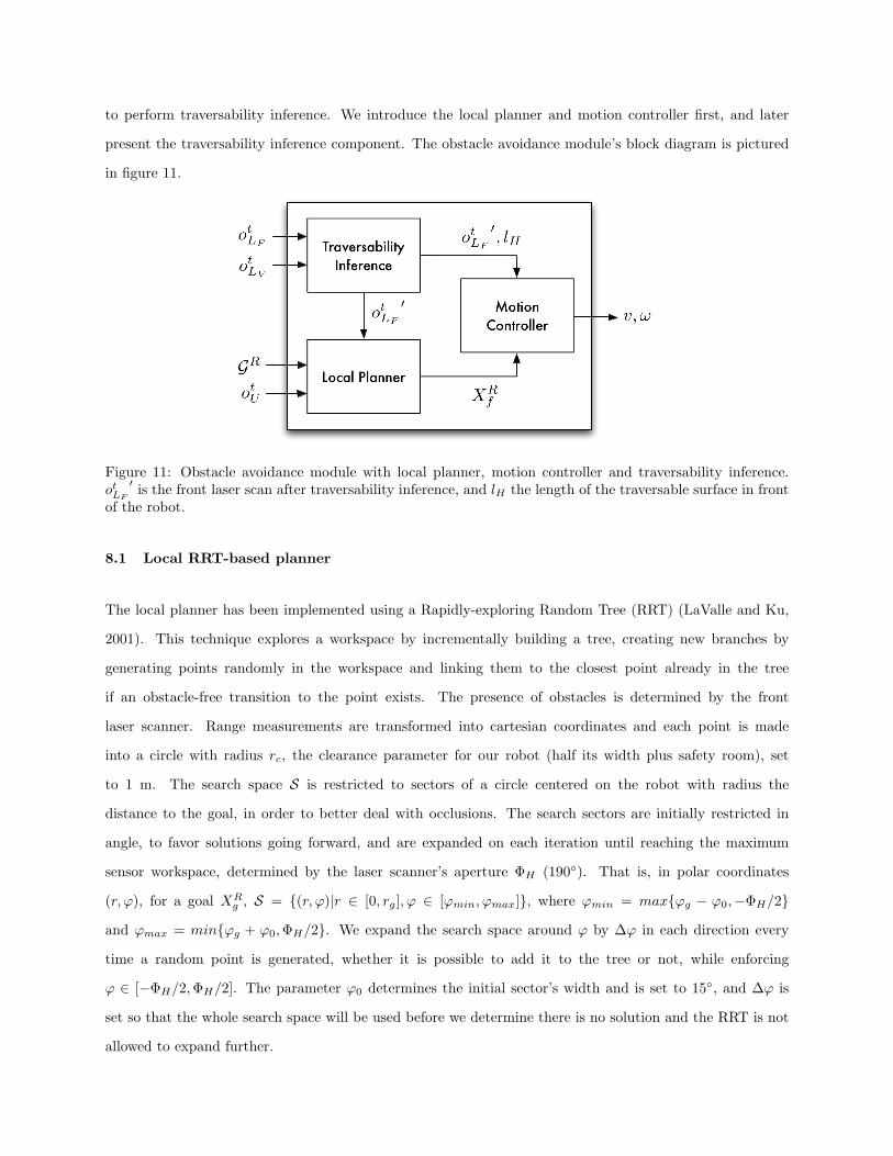
to perform traversability inference. We introduce the local planner and motion controller first, and later
present the traversability inference component. The obstacle avoidance module’s block diagram is pictured
in figure 11.
Traversability Inference
Local Planner
Motion Controller
Figure 11: Obstacle avoidance module with local planner, motion controller and traversability inference.otLF
′ is the front laser scan after traversability inference, and lH the length of the traversable surface in frontof the robot.
8.1 Local RRT-based planner
The local planner has been implemented using a Rapidly-exploring Random Tree (RRT) (LaValle and Ku,
2001). This technique explores a workspace by incrementally building a tree, creating new branches by
generating points randomly in the workspace and linking them to the closest point already in the tree
if an obstacle-free transition to the point exists. The presence of obstacles is determined by the front
laser scanner. Range measurements are transformed into cartesian coordinates and each point is made
into a circle with radius rc, the clearance parameter for our robot (half its width plus safety room), set
to 1 m. The search space S is restricted to sectors of a circle centered on the robot with radius the
distance to the goal, in order to better deal with occlusions. The search sectors are initially restricted in
angle, to favor solutions going forward, and are expanded on each iteration until reaching the maximum
sensor workspace, determined by the laser scanner’s aperture ΦH (190◦). That is, in polar coordinates
(r, ϕ), for a goal XRg , S = {(r, ϕ)|r ∈ [0, rg], ϕ ∈ [ϕmin, ϕmax]}, where ϕmin = max{ϕg − ϕ0,−ΦH/2}
and ϕmax = min{ϕg + ϕ0,ΦH/2}. We expand the search space around ϕ by ∆ϕ in each direction every
time a random point is generated, whether it is possible to add it to the tree or not, while enforcing
ϕ ∈ [−ΦH/2,ΦH/2]. The parameter ϕ0 determines the initial sector’s width and is set to 15◦, and ∆ϕ is
set so that the whole search space will be used before we determine there is no solution and the RRT is not
allowed to expand further.
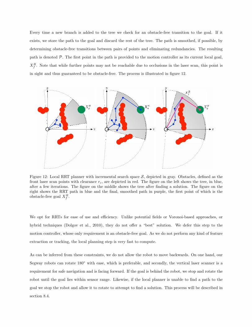
Every time a new branch is added to the tree we check for an obstacle-free transition to the goal. If it
exists, we store the path to the goal and discard the rest of the tree. The path is smoothed, if possible, by
determining obstacle-free transitions between pairs of points and eliminating redundancies. The resulting
path is denoted P. The first point in the path is provided to the motion controller as its current local goal,
XRf . Note that while further points may not be reachable due to occlusions in the laser scan, this point is
in sight and thus guaranteed to be obstacle-free. The process is illustrated in figure 12.
Figure 12: Local RRT planner with incremental search space S, depicted in gray. Obstacles, defined as thefront laser scan points with clearance rc, are depicted in red. The figure on the left shows the tree, in blue,after a few iterations. The figure on the middle shows the tree after finding a solution. The figure on theright shows the RRT path in blue and the final, smoothed path in purple, the first point of which is theobstacle-free goal XR
f .
We opt for RRTs for ease of use and efficiency. Unlike potential fields or Voronoi-based approaches, or
hybrid techniques (Dolgov et al., 2010), they do not offer a “best” solution. We defer this step to the
motion controller, whose only requirement is an obstacle-free goal. As we do not perform any kind of feature
extraction or tracking, the local planning step is very fast to compute.
As can be inferred from these constraints, we do not allow the robot to move backwards. On one hand, our
Segway robots can rotate 180◦ with ease, which is preferable, and secondly, the vertical laser scanner is a
requirement for safe navigation and is facing forward. If the goal is behind the robot, we stop and rotate the
robot until the goal lies within sensor range. Likewise, if the local planner is unable to find a path to the
goal we stop the robot and allow it to rotate to attempt to find a solution. This process will be described in
section 8.4.
8.2 Motion controller
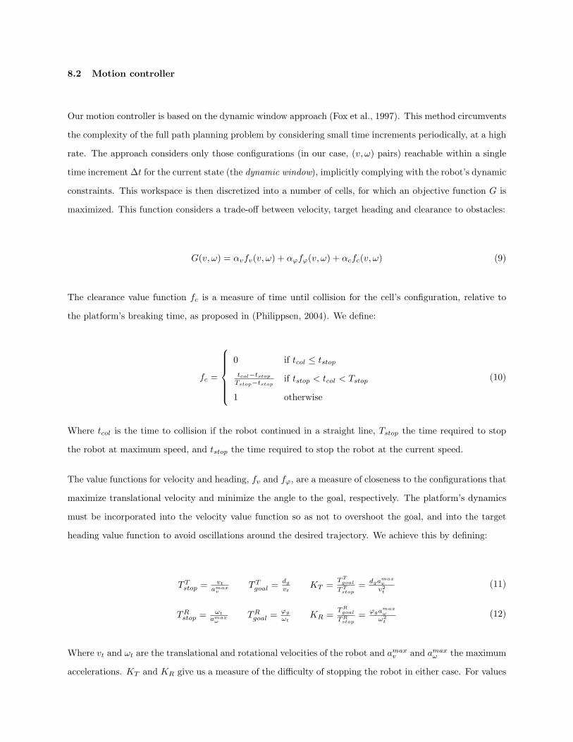
Our motion controller is based on the dynamic window approach (Fox et al., 1997). This method circumvents
the complexity of the full path planning problem by considering small time increments periodically, at a high
rate. The approach considers only those configurations (in our case, (v, ω) pairs) reachable within a single
time increment ∆t for the current state (the dynamic window), implicitly complying with the robot’s dynamic
constraints. This workspace is then discretized into a number of cells, for which an objective function G is
maximized. This function considers a trade-off between velocity, target heading and clearance to obstacles:
G(v, ω) = αvfv(v, ω) + αϕfϕ(v, ω) + αcfc(v, ω) (9)
The clearance value function fc is a measure of time until collision for the cell’s configuration, relative to
the platform’s breaking time, as proposed in (Philippsen, 2004). We define:
fc =
0 if tcol ≤ tstoptcol−tstopTstop−tstop if tstop < tcol < Tstop
1 otherwise
(10)
Where tcol is the time to collision if the robot continued in a straight line, Tstop the time required to stop
the robot at maximum speed, and tstop the time required to stop the robot at the current speed.
The value functions for velocity and heading, fv and fϕ, are a measure of closeness to the configurations that
maximize translational velocity and minimize the angle to the goal, respectively. The platform’s dynamics
must be incorporated into the velocity value function so as not to overshoot the goal, and into the target
heading value function to avoid oscillations around the desired trajectory. We achieve this by defining:
TTstop = vtamaxv
TTgoal = dgvt
KT = TTgoalTTstop
= dgamaxv
v2t(11)
TRstop = ωtamaxω
TRgoal = ϕgωt
KR = TRgoalTRstop
= ϕgamaxω
ω2t
(12)
Where vt and ωt are the translational and rotational velocities of the robot and amaxv and amaxω the maximum
accelerations. KT and KR give us a measure of the difficulty of stopping the robot in either case. For values
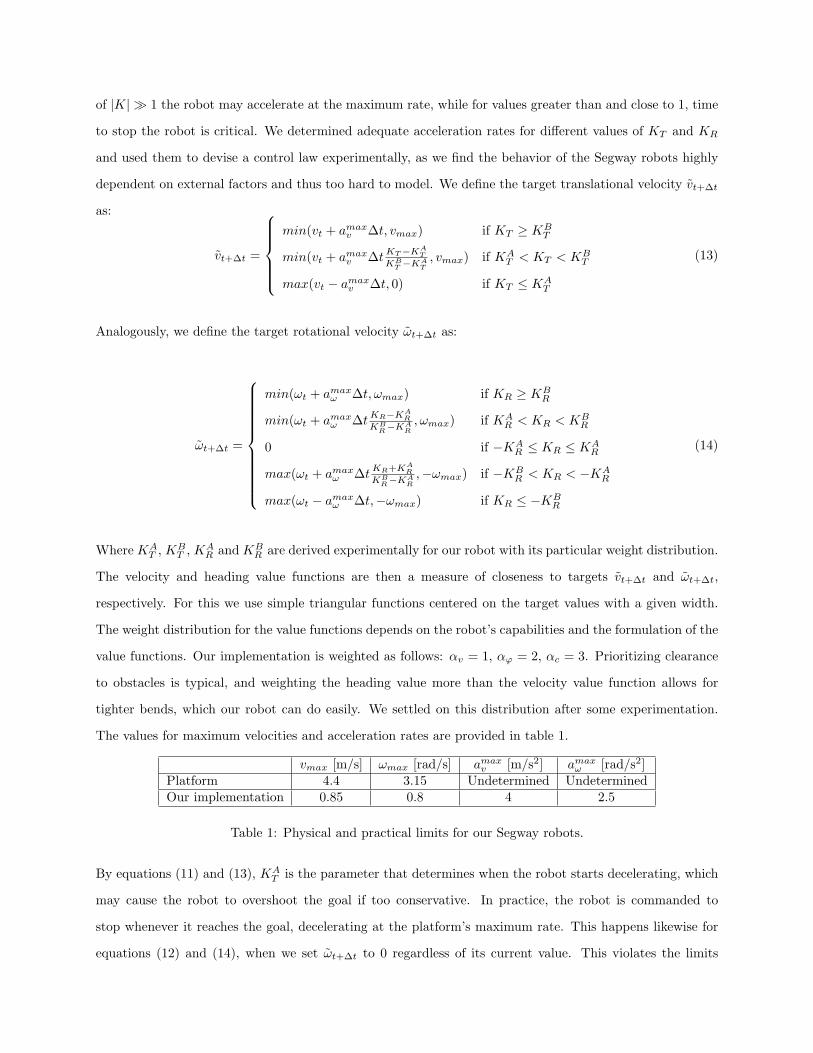
of |K| � 1 the robot may accelerate at the maximum rate, while for values greater than and close to 1, time
to stop the robot is critical. We determined adequate acceleration rates for different values of KT and KR
and used them to devise a control law experimentally, as we find the behavior of the Segway robots highly
dependent on external factors and thus too hard to model. We define the target translational velocity vt+∆t
as:
vt+∆t =
min(vt + amaxv ∆t, vmax) if KT ≥ KB
T
min(vt + amaxv ∆tKT−KAT
KBT −KA
T
, vmax) if KAT < KT < KB
T
max(vt − amaxv ∆t, 0) if KT ≤ KAT
(13)
Analogously, we define the target rotational velocity ωt+∆t as:
ωt+∆t =
min(ωt + amaxω ∆t, ωmax) if KR ≥ KBR
min(ωt + amaxω ∆tKR−KAR
KBR−KA
R
, ωmax) if KAR < KR < KB
R
0 if −KAR ≤ KR ≤ KA
R
max(ωt + amaxω ∆tKR+KAR
KBR−KA
R
,−ωmax) if −KBR < KR < −KA
R
max(ωt − amaxω ∆t,−ωmax) if KR ≤ −KBR
(14)
Where KAT , KB
T , KAR and KB
R are derived experimentally for our robot with its particular weight distribution.
The velocity and heading value functions are then a measure of closeness to targets vt+∆t and ωt+∆t,
respectively. For this we use simple triangular functions centered on the target values with a given width.
The weight distribution for the value functions depends on the robot’s capabilities and the formulation of the
value functions. Our implementation is weighted as follows: αv = 1, αϕ = 2, αc = 3. Prioritizing clearance
to obstacles is typical, and weighting the heading value more than the velocity value function allows for
tighter bends, which our robot can do easily. We settled on this distribution after some experimentation.
The values for maximum velocities and acceleration rates are provided in table 1.
vmax [m/s] ωmax [rad/s] amaxv [m/s2] amaxω [rad/s2]Platform 4.4 3.15 Undetermined UndeterminedOur implementation 0.85 0.8 4 2.5
Table 1: Physical and practical limits for our Segway robots.
By equations (11) and (13), KAT is the parameter that determines when the robot starts decelerating, which
may cause the robot to overshoot the goal if too conservative. In practice, the robot is commanded to
stop whenever it reaches the goal, decelerating at the platform’s maximum rate. This happens likewise for
equations (12) and (14), when we set ωt+∆t to 0 regardless of its current value. This violates the limits
listed in table 1, but not the platform limits, thus still observing the dynamic window principle. We find
this allows for better control of the platform.
8.3 Traversability inference
False obstacles due to, for instance, ramps may be detected by incorporating the localization estimate and
using the 3D map to identify the situation, but this solution dangerously couples the robot’s reactive behavior
to the robustness of the localization process. This would compromise the safety of our navigation system.
Thus, our approach is based on the vertical laser scanner, used to infer whether the robot can traverse this
region of space. It also enables the robot to detect some obstacles outside the field of view of the horizontal
laser scanners.
The campus features three different kinds of traversable surfaces: flat, sloped with a relatively even incline,
and transitions from one to the other. The Gracia environment does not feature noticeable changes in
inclination, while being sloped throughout. The vertical laser observations in these environments can thus
be modeled with one or two line segments. Linear regressions are extracted from the sensor data by least
squares fitting, using the average regression error to determine its quality. Prior to this computation, the
vertical laser scan is pre-processed by removing points beyond the range of the obstacle avoidance module
(8 m), or due to interference with the robot chassis. The inference process is divided into three steps, executed
in order, and is terminated whenever one of these steps produces a satisfactory solution. We consider:
1. A single regression using all data.
2. Two regressions, using all data sorted over x and divided into two sets by a threshold, for a set of
thresholds over x, until conditions are met.
3. A single regression, iteratively removing the points farthest away from the robot over x, until con-
ditions are met.
In any case, a maximum regression error and a minimum regression length must be satisfied. In the second
case two additional conditions are enforced in order to ensure the compatibility between segments: the
vertical gap and the angular difference between regressions must be sufficiently small. These thresholds were
determined empirically for our sensors at the campus environment.
This inference process enables the robots to enter and traverse ramps by removing points from the front
laser scan incorrectly indicating the presence of obstacles prior to local planning. To do this, we use the
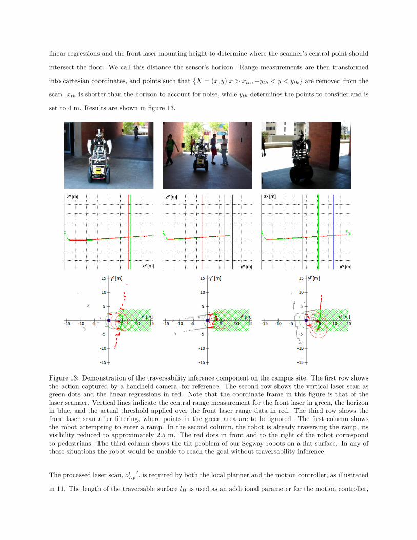
linear regressions and the front laser mounting height to determine where the scanner’s central point should
intersect the floor. We call this distance the sensor’s horizon. Range measurements are then transformed
into cartesian coordinates, and points such that {X = (x, y)|x > xth,−yth < y < yth} are removed from the
scan. xth is shorter than the horizon to account for noise, while yth determines the points to consider and is
set to 4 m. Results are shown in figure 13.
Figure 13: Demonstration of the traversability inference component on the campus site. The first row showsthe action captured by a handheld camera, for reference. The second row shows the vertical laser scan asgreen dots and the linear regressions in red. Note that the coordinate frame in this figure is that of thelaser scanner. Vertical lines indicate the central range measurement for the front laser in green, the horizonin blue, and the actual threshold applied over the front laser range data in red. The third row shows thefront laser scan after filtering, where points in the green area are to be ignored. The first column showsthe robot attempting to enter a ramp. In the second column, the robot is already traversing the ramp, itsvisibility reduced to approximately 2.5 m. The red dots in front and to the right of the robot correspondto pedestrians. The third column shows the tilt problem of our Segway robots on a flat surface. In any ofthese situations the robot would be unable to reach the goal without traversability inference.
The processed laser scan, otLF′, is required by both the local planner and the motion controller, as illustrated
in 11. The length of the traversable surface lH is used as an additional parameter for the motion controller,
limiting the translational speed or directly stopping the robot. The robot is also commanded to stop if the
slope is too steep for the platform. Staircases are easy to discriminate when seen from the bottom, but from
the top the laser’s accuracy presents a problem and some observations are close enough to those of a ramp
to fall under the threshold. The staircase’s steep incline is then used to disambiguate.
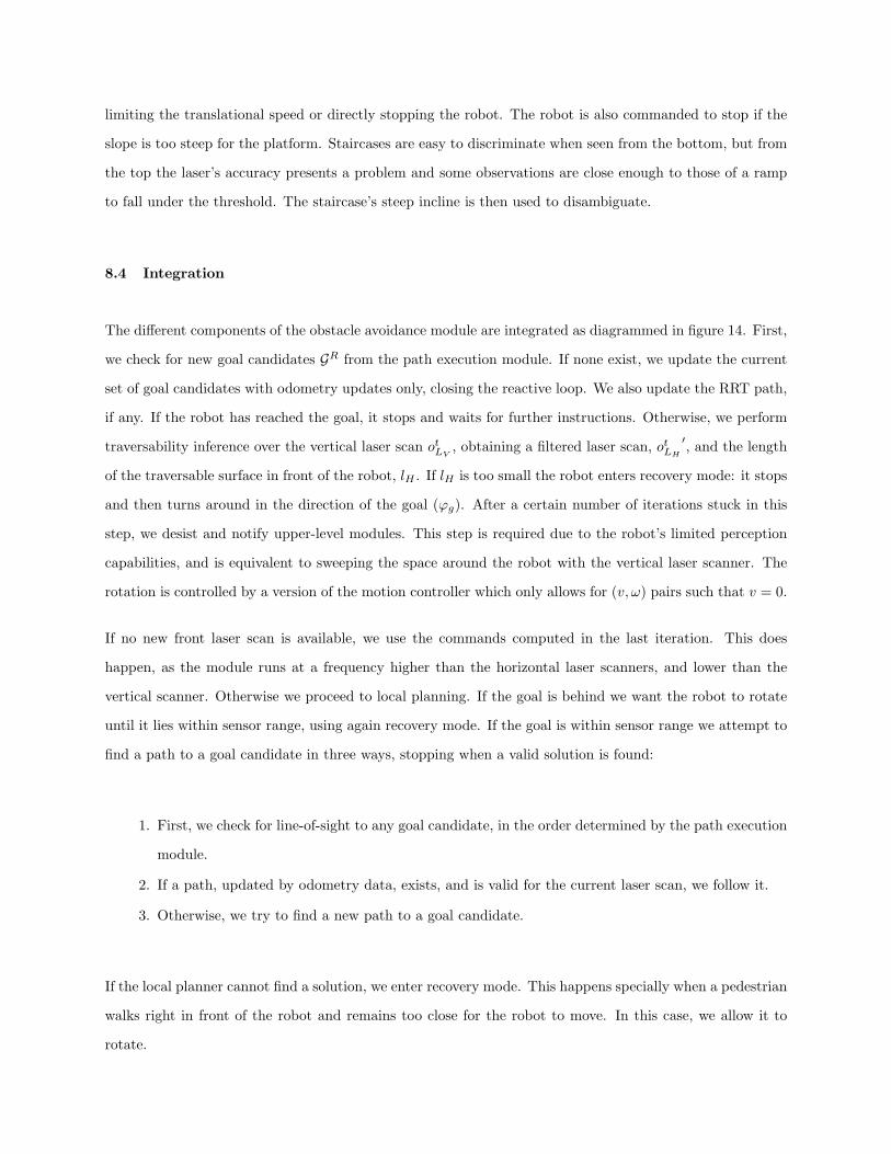
8.4 Integration
The different components of the obstacle avoidance module are integrated as diagrammed in figure 14. First,
we check for new goal candidates GR from the path execution module. If none exist, we update the current
set of goal candidates with odometry updates only, closing the reactive loop. We also update the RRT path,
if any. If the robot has reached the goal, it stops and waits for further instructions. Otherwise, we perform
traversability inference over the vertical laser scan otLV , obtaining a filtered laser scan, otLH′, and the length
of the traversable surface in front of the robot, lH . If lH is too small the robot enters recovery mode: it stops
and then turns around in the direction of the goal (ϕg). After a certain number of iterations stuck in this
step, we desist and notify upper-level modules. This step is required due to the robot’s limited perception
capabilities, and is equivalent to sweeping the space around the robot with the vertical laser scanner. The
rotation is controlled by a version of the motion controller which only allows for (v, ω) pairs such that v = 0.
If no new front laser scan is available, we use the commands computed in the last iteration. This does
happen, as the module runs at a frequency higher than the horizontal laser scanners, and lower than the
vertical scanner. Otherwise we proceed to local planning. If the goal is behind we want the robot to rotate
until it lies within sensor range, using again recovery mode. If the goal is within sensor range we attempt to
find a path to a goal candidate in three ways, stopping when a valid solution is found:
1. First, we check for line-of-sight to any goal candidate, in the order determined by the path execution
module.
2. If a path, updated by odometry data, exists, and is valid for the current laser scan, we follow it.
3. Otherwise, we try to find a new path to a goal candidate.
If the local planner cannot find a solution, we enter recovery mode. This happens specially when a pedestrian
walks right in front of the robot and remains too close for the robot to move. In this case, we allow it to
rotate.
Goalachieved
Goalbehind
Line ofsight to k-th goal
candidate
YesNo
Yes
Yes
Yes
Yes
Yes
Yes
Yes
No
No
No
No
No
No
No
Figure 14: Obstacle avoidance module diagram. Parameters are: goal candidates from the path executionmodule GR,t, laser scans otLF and otLV , and odometry updates otU . The process stores the last set of goalcandidates GR,t−1 and the last path computed by the local planner PR,t−1. Blocks painted blue, green andred belong to the traversability inference algorithm, the local planner and the motion controller, respectively.Gray blocks are process logic.
9 Experiments and assessment of results
The navigation system was validated over the course of four experimental sessions, one on the Gracia site
and three at the Campus. An external computer, connected to the on-board computer via wireless, was
used to send manual go-to requests (XY coordinates over the map) to the navigation system, and for on-line
monitoring using our GUI. Note that these are high-level requests, equivalent to “send a robot to the south-
east door of the A5 building”. Goals in the experiments include both long distances across the campus (the
longest possible path between two points being around 150 m), and goals closer to each other to force the
robot (and thus the path planning algorithm) through more complex situations such as around the trees in
the square or around the columns in the A5/A6 buildings. Requests were often chained to keep the robot in
motion, sending the robot to a new location just before reaching the current goal. We typically chose closer
goals to keep some control over the trajectories and have the robot explore all of the area.
Runtime for all experiments added up to 2.3 hours, with over 6 km of autonomous navigation. We set a
speed limit of 0.75 m/s for the first session, and increased it to 0.85 m/s for the following three sessions –
note that this is a soft limit, and the robot often travels faster due to its self-balancing behavior. We used
Tibi and Dabo without distinction.
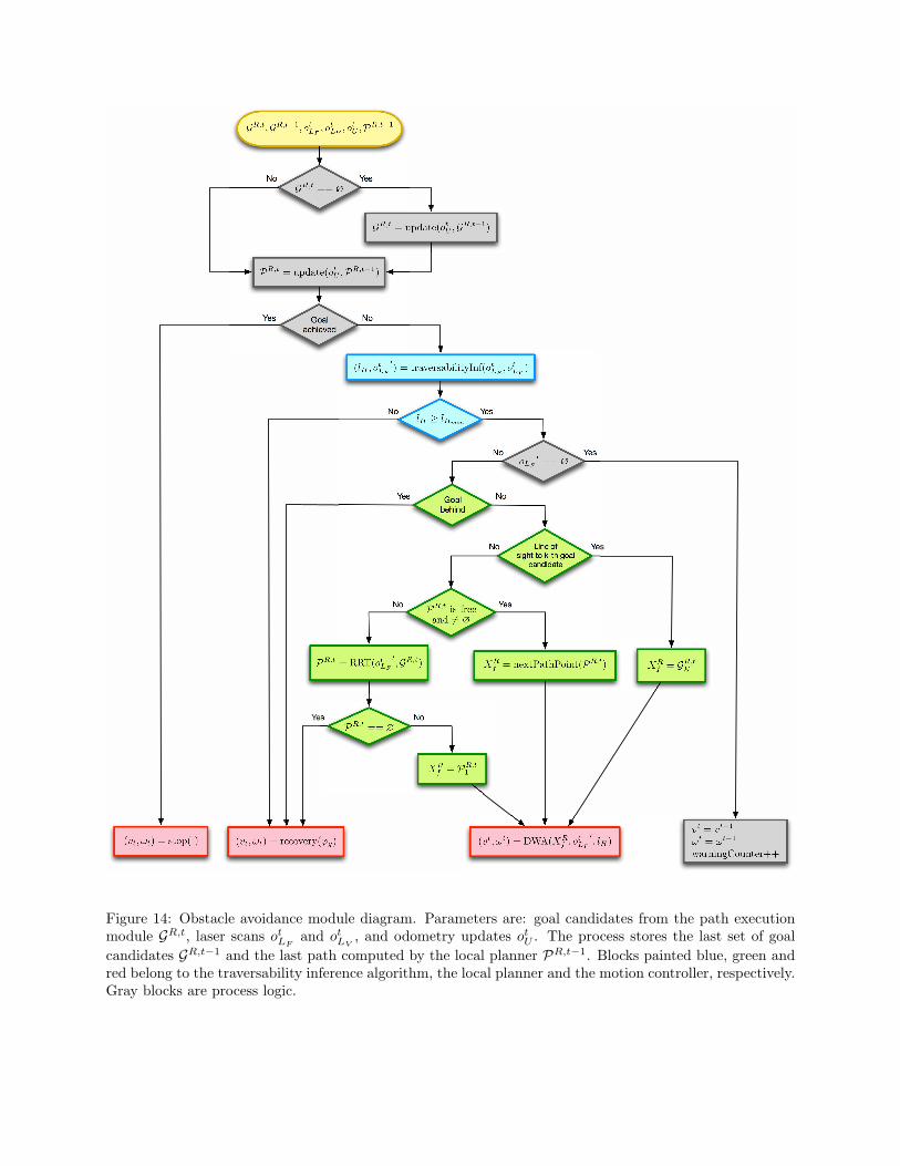
Results are displayed in tables 2 and 3. Table 2 lists the navigation distance D, as estimated by the
localization module, and the total navigation time tnav, understood as that spent with the robot attending
a go-to request. This measure is divided in time spent on obstacle-free navigation tfree, active obstacle
avoidance tOA, safety stops tstop, and rotation on recovery mode trot. The ratio ROA is a measure of the
time spent avoiding obstacles, computed as ROA = (tOA + tstop + trot)/tnav, and v is an estimation of the
average translational speed computed using the previous values, v = D/tnav. Table 3 displays the number
of requests, failures, and success rate, as well as the average navigated distance per request dreq.
Table 2: Experimental results (1)Place & Date D [m] tnav [s] tfree [s] tOA [s] tstop [s] trot [s] ROA [%] v [m/s]
Gracia, 20-May-2010 777.7 1107.9 978.9 40.1 15 73.9 13.2 0.71Campus, 3-Jun-2010 858.5 1056.2 903.3 91.9 19.9 41.1 14.5 0.81Campus, 22-Jun-2010 2481.8 3426.3 2481.1 541.3 174.3 229.6 27.6 0.72Campus, 23-Jun-2010 2252.5 2727.3 2325.8 186.8 75.4 139.3 14.7 0.83
Accumulated 6370.5 8317.7 6689.1 860.1 284.6 483.9 19.6 0.77
We were allowed three days (mornings only) to conduct experiments at the Gracia site, the last of which
was dedicated to a public demonstration, and so the scope of that session is limited, totaling less than
1 km of autonomous navigation. Even so it must be noted that, due to time constraints, these experiments

Table 3: Experimental results (2)Place & Date Requests [#] dreq [m] Errors [#] Success rate [%]
Gracia, 20-May-2010 33 23.6 0 100Campus, 3-Jun-2010 23 37.3 0 100Campus, 22-Jun-2010 55 45.1 0 100Campus, 23-Jun-2010 60 37.5 2 96.7
Accumulated 171 37.3 2 98.8
were conducted with little to no prior in-site testing. Moreover, while part of the area was fenced, many
pedestrians and bicyclists disregarded instructions and crossed the area anyway. This proves the robustness
of our navigation system in new environments under similar conditions.
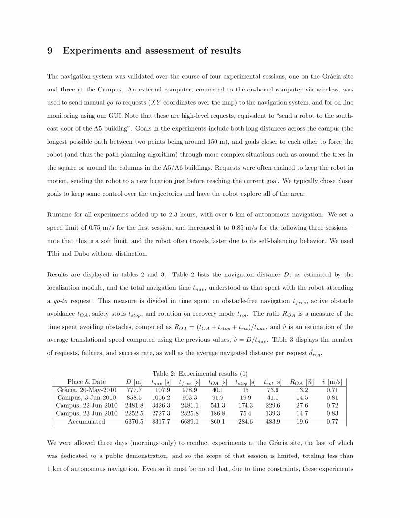
The four runs are plotted in figure 15. For the session at the Gracia site, we fenced the rightmost passageway
and allowed pedestrians and bicyclists to use the one on the left. The rest of the area was left as-is except for
four fences placed below the monument, at y = 20 (fig. 15, top left), as a safety measure. The second session,
already at the Campus site, starts at (90,38), and ends at (17,69) when the robot encounters a large section
occupied by public works and thus unmapped. In the third session we ventured once to the passageway
between C and D buildings, which is on the verge of the experimental area and was roughly mapped, and
hence did not revisit. We also had the opportunity to navigate the narrow passageway to the right of the FIB
square, which is usually occupied by the cafeteria’s terrace. Please note that areas where the localization
estimate is within a building, such as for A5, A6 and C6, are covered (fig. 2, picture number 2).
The fourth run contains the only two errors we encountered. Both are related to the localization algorithm,
and were mainly due to features of the terrain. Subsection 9.1 analyzes these two failures in detail.
The first and second sessions are documented by one video each, available on the following website: http:
//www.iri.upc.edu/people/etrulls/jfr10. The video for the second session contains the session in its
entirety. Figure 16 provides a sample screenshot with an explanation of the different data shown.
All navigation processes run concurrently on a single laptop. The localization process runs at 5 Hz, and
the obstacle avoidance process runs at 10 Hz. Traversability inference is typically computed in less than
1 ms, while the local planner takes 1-10 ms per iteration, up to about 50 ms for the worst-case scenario (five
goal candidates, no solution). The computational cost for the dynamic window computation depends on its
granularity, taking an average of 10 ms for 175 cells. The path execution module carries a negligible compu-
tational load, and the path planning module is only executed upon a go-to request and takes approximately
one second, which does not interfere in real-time navigation.
Figure 15: Localization results for the four experimental sessions. Red circles in the bottom right figuremark failure points.
9.1 Failure Analysis
Having failures gives us the chance to learn, advance and improve our system. Therefore, this subsection
provides insights to the two localization failures that occurred during the last session, at the Campus site.
This analysis was made possible by the off-line study of the logged data for that session, automatically stored
by our software framework. Our localization module can be run off-line using dummy sensors, which publish
logged sensor data under the same interfaces as during on-line executions, while keeping synchronization.
This allows us to run new real-time, off-line executions of the localization process with the data collected
during on-line executions.
The first failure happened approximately at XY point (90,50). The robot was traveling from left to right
along y = 38 and turned to its left to go up the ramp at x = 90 (fig. 15). The turning point can be seen
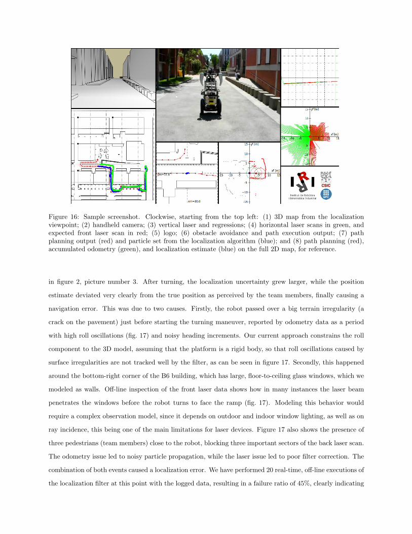
Figure 16: Sample screenshot. Clockwise, starting from the top left: (1) 3D map from the localizationviewpoint; (2) handheld camera; (3) vertical laser and regressions; (4) horizontal laser scans in green, andexpected front laser scan in red; (5) logo; (6) obstacle avoidance and path execution output; (7) pathplanning output (red) and particle set from the localization algorithm (blue); and (8) path planning (red),accumulated odometry (green), and localization estimate (blue) on the full 2D map, for reference.
in figure 2, picture number 3. After turning, the localization uncertainty grew larger, while the position
estimate deviated very clearly from the true position as perceived by the team members, finally causing a
navigation error. This was due to two causes. Firstly, the robot passed over a big terrain irregularity (a
crack on the pavement) just before starting the turning maneuver, reported by odometry data as a period
with high roll oscillations (fig. 17) and noisy heading increments. Our current approach constrains the roll
component to the 3D model, assuming that the platform is a rigid body, so that roll oscillations caused by
surface irregularities are not tracked well by the filter, as can be seen in figure 17. Secondly, this happened
around the bottom-right corner of the B6 building, which has large, floor-to-ceiling glass windows, which we
modeled as walls. Off-line inspection of the front laser data shows how in many instances the laser beam
penetrates the windows before the robot turns to face the ramp (fig. 17). Modeling this behavior would
require a complex observation model, since it depends on outdoor and indoor window lighting, as well as on
ray incidence, this being one of the main limitations for laser devices. Figure 17 also shows the presence of
three pedestrians (team members) close to the robot, blocking three important sectors of the back laser scan.
The odometry issue led to noisy particle propagation, while the laser issue led to poor filter correction. The
combination of both events caused a localization error. We have performed 20 real-time, off-line executions of
the localization filter at this point with the logged data, resulting in a failure ratio of 45%, clearly indicating
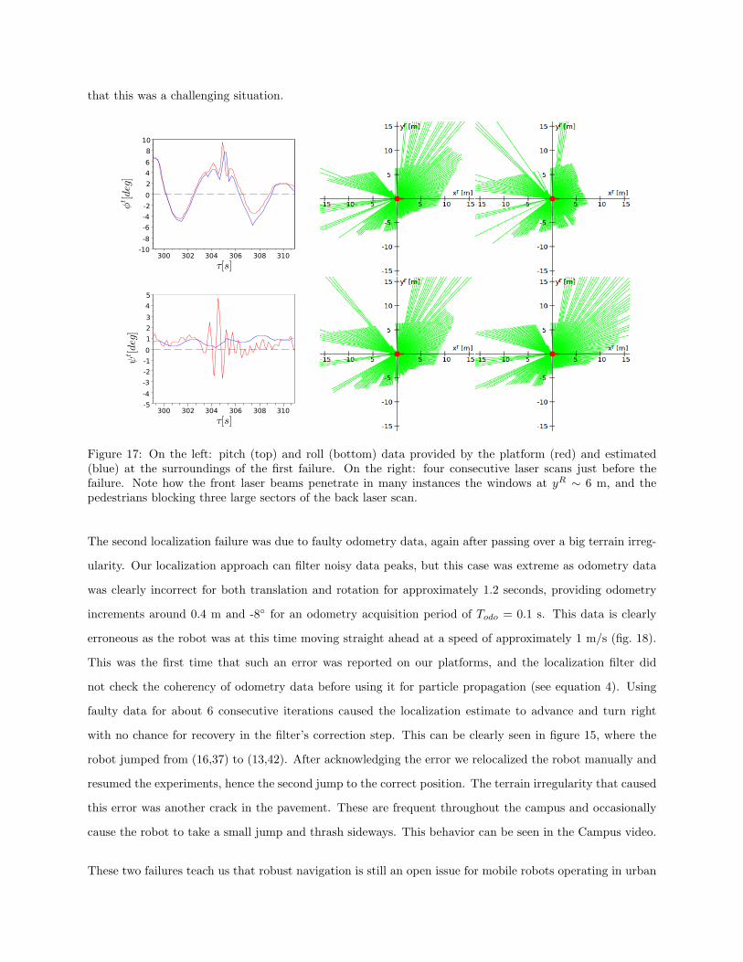
that this was a challenging situation.
Figure 17: On the left: pitch (top) and roll (bottom) data provided by the platform (red) and estimated(blue) at the surroundings of the first failure. On the right: four consecutive laser scans just before thefailure. Note how the front laser beams penetrate in many instances the windows at yR ∼ 6 m, and thepedestrians blocking three large sectors of the back laser scan.
The second localization failure was due to faulty odometry data, again after passing over a big terrain irreg-
ularity. Our localization approach can filter noisy data peaks, but this case was extreme as odometry data
was clearly incorrect for both translation and rotation for approximately 1.2 seconds, providing odometry
increments around 0.4 m and -8◦ for an odometry acquisition period of Todo = 0.1 s. This data is clearly
erroneous as the robot was at this time moving straight ahead at a speed of approximately 1 m/s (fig. 18).
This was the first time that such an error was reported on our platforms, and the localization filter did
not check the coherency of odometry data before using it for particle propagation (see equation 4). Using
faulty data for about 6 consecutive iterations caused the localization estimate to advance and turn right
with no chance for recovery in the filter’s correction step. This can be clearly seen in figure 15, where the
robot jumped from (16,37) to (13,42). After acknowledging the error we relocalized the robot manually and
resumed the experiments, hence the second jump to the correct position. The terrain irregularity that caused
this error was another crack in the pavement. These are frequent throughout the campus and occasionally
cause the robot to take a small jump and thrash sideways. This behavior can be seen in the Campus video.
These two failures teach us that robust navigation is still an open issue for mobile robots operating in urban
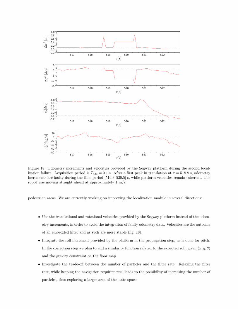
Figure 18: Odometry increments and velocities provided by the Segway platform during the second local-ization failure. Acquisition period is Todo = 0.1 s. After a first peak in translation at τ = 518.8 s, odometryincrements are faulty during the time period [519.3, 520.5] s, while platform velocities remain coherent. Therobot was moving straight ahead at approximately 1 m/s.
pedestrian areas. We are currently working on improving the localization module in several directions:
• Use the translational and rotational velocities provided by the Segway platform instead of the odom-
etry increments, in order to avoid the integration of faulty odometry data. Velocities are the outcome
of an embedded filter and as such are more stable (fig. 18).
• Integrate the roll increment provided by the platform in the propagation step, as is done for pitch.
In the correction step we plan to add a similarity function related to the expected roll, given (x, y, θ)
and the gravity constraint on the floor map.
• Investigate the trade-off between the number of particles and the filter rate. Relaxing the filter
rate, while keeping the navigation requirements, leads to the possibility of increasing the number of
particles, thus exploring a larger area of the state space.
An early, improved version of the particle filter is giving promising results after a series of real-time, off-line
executions when the robot passes over the two failure situations.
10 Lessons learnt and future work
Despite many recent advances, reliable autonomous navigation in urban, pedestrian environments remains
a major challenge in robotics. This paper presents a solution geared towards two-wheeled robots, highly
mobile and with a small footprint, and deals effectively with problems in both perception and control due to
their self-balancing behavior. It has been extensively tested in two different urban scenarios, covering over
6 km with a 99% success rate.
The main issue to be addressed in the future is one of perception. We rely on 2D laser scanners for
localization and obstacle avoidance, because (1) they provide an immediate perception stage with no need
for feature extraction, and (2) they are robust to varying illumination conditions. On the downside, they are
by definition limited to a 2D plane. This impairs the visibility of horizontal laser scanners on urban scenarios
with ramps, which has been addressed by means of the vertical laser scanner and the traversability inference
algorithm. But obstacles outside either plane remain a problem. We find in practice that objects or terrain
features lying low on the floor, such as curbs or steps, are the most problematic, as the vertical scanner
can only sense forward and the wheels extend approximately 30 cm to either side. 3D laser scanners are
costly and bulky, and current time-of-flight cameras are not usable under direct sunlight. We plan to explore
the use of multiple laser scanners tilted to the floor to build local obstacle maps, using feature matching
and/or in conjunction with the localization estimate. Note that with this configuration the platform’s tilt
would again pose a problem, and the mobility of the robot may be reduced because of blind spots when
turning on its axis, as explained in section 8. We would also have to deal with occlusions and dynamic
obstacles explicitly. We also plan to explore the use of stereo cameras in hybrid laser-camera solutions, for
both localization and obstacle avoidance.
Future research also includes the identification and tracking of moving objects for better motion planning
on the local domain, and the extension of the path planning and path execution algorithms from 2D to
3D. The latter would enable us to deal with multi-level environments: while the Campus setting presents
great variations in height, there is at most one traversable surface for a (x, y) point. Higher-level extensions
include the segmentation of unmapped objects for incorporation to the 3D map, by extending past and
current work on mapping the Campus area (Valencia et al., 2009). The robot may then deal with situations
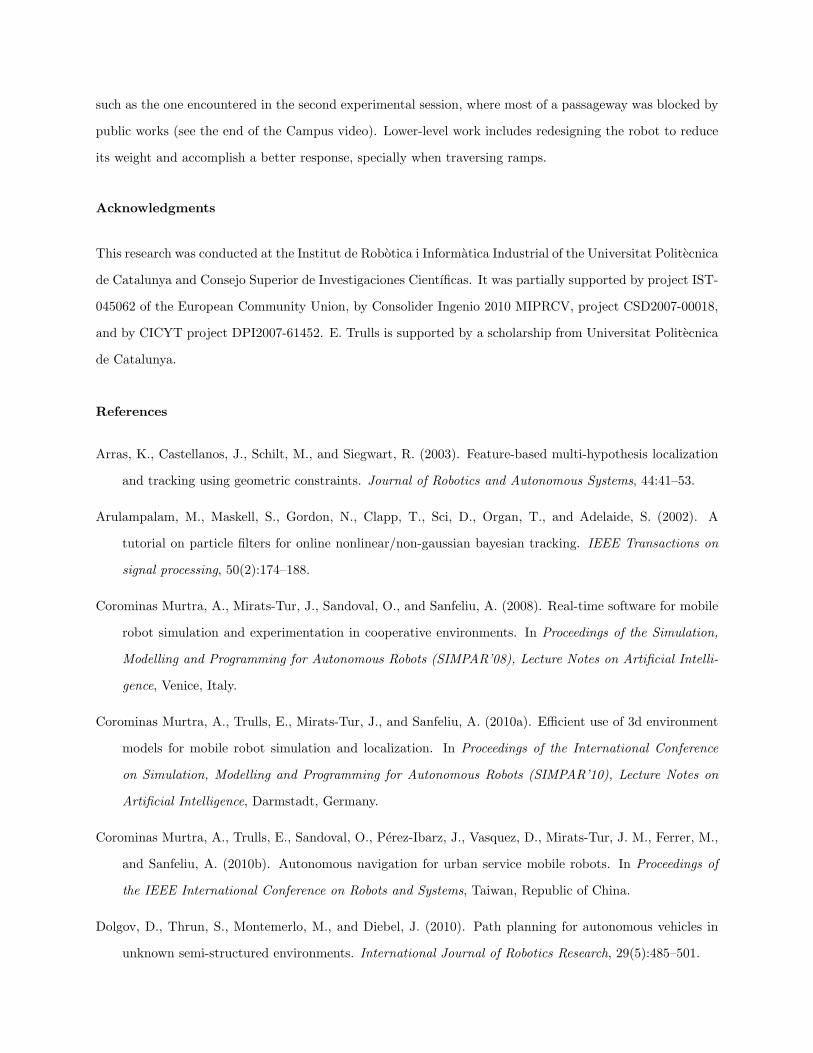
such as the one encountered in the second experimental session, where most of a passageway was blocked by
public works (see the end of the Campus video). Lower-level work includes redesigning the robot to reduce
its weight and accomplish a better response, specially when traversing ramps.
Acknowledgments
This research was conducted at the Institut de Robotica i Informatica Industrial of the Universitat Politecnica
de Catalunya and Consejo Superior de Investigaciones Cientıficas. It was partially supported by project IST-
045062 of the European Community Union, by Consolider Ingenio 2010 MIPRCV, project CSD2007-00018,
and by CICYT project DPI2007-61452. E. Trulls is supported by a scholarship from Universitat Politecnica
de Catalunya.
References
Arras, K., Castellanos, J., Schilt, M., and Siegwart, R. (2003). Feature-based multi-hypothesis localization
and tracking using geometric constraints. Journal of Robotics and Autonomous Systems, 44:41–53.
Arulampalam, M., Maskell, S., Gordon, N., Clapp, T., Sci, D., Organ, T., and Adelaide, S. (2002). A
tutorial on particle filters for online nonlinear/non-gaussian bayesian tracking. IEEE Transactions on
signal processing, 50(2):174–188.
Corominas Murtra, A., Mirats-Tur, J., Sandoval, O., and Sanfeliu, A. (2008). Real-time software for mobile
robot simulation and experimentation in cooperative environments. In Proceedings of the Simulation,
Modelling and Programming for Autonomous Robots (SIMPAR’08), Lecture Notes on Artificial Intelli-
gence, Venice, Italy.
Corominas Murtra, A., Trulls, E., Mirats-Tur, J., and Sanfeliu, A. (2010a). Efficient use of 3d environment
models for mobile robot simulation and localization. In Proceedings of the International Conference
on Simulation, Modelling and Programming for Autonomous Robots (SIMPAR’10), Lecture Notes on
Artificial Intelligence, Darmstadt, Germany.
Corominas Murtra, A., Trulls, E., Sandoval, O., Perez-Ibarz, J., Vasquez, D., Mirats-Tur, J. M., Ferrer, M.,
and Sanfeliu, A. (2010b). Autonomous navigation for urban service mobile robots. In Proceedings of
the IEEE International Conference on Robots and Systems, Taiwan, Republic of China.
Dolgov, D., Thrun, S., Montemerlo, M., and Diebel, J. (2010). Path planning for autonomous vehicles in
unknown semi-structured environments. International Journal of Robotics Research, 29(5):485–501.
Doucet, A., de Freitas, N., and Gordon, N. (2001). Sequential Monte Carlo Methods in Practice. Springer
Science.
Fox, D., Burgard, W., and Thrun, S. (1997). The dynamic window approach to collision avoidance. Robotics
& Automation Magazine, 4(1):23–33.
Georgiev, A. and Allen, P. (2004). Localization methods for a mobile robot in urban environments. IEEE
Transactions on Robotics and Automation, 20(5).
Haddad, H., Khatib, M., Lacroix, S., and Chatila, R. (1998). Reactive navigation in outdoor environments
using potential fields. In Proceedings of the IEEE International Conference on Robotics and Automation.
Khatib, M. and Chatila, R. (1995). An extended potential field approach for mobile robot sensor-based
motions. In Proceedings of Intelligent Autonomous Systems, pages 490–496.
Khatib, O. (1986). Real-time obstacle avoidance for manipulators and mobile robots. The International
Journal of Robotics Research, 5(1):90–98.
Latombe, J. (1991). Robot Motion Planning. Kluwer Academic Publishers.
LaValle, S. and Ku, J. (2001). Rapidly-exploring random trees: Progress and prospects. In Algorithmic and
Computational Robotics: New Directions. Fourth Workshop on the Algorithmic Foundations of Robotics.
AK Peters, Ltd.
Levinson, J., Montemerlo, M., and Thrun, S. (2007). Map-based precision vehicle localization in urban
environments. In Proceedings of the Robotics: Science and Systems Conference, Atlanta, USA.
Luettel, T., Himmelsbach, M., Hundelshausen, F. V., Manz, M., Mueller, A., and Wuensche, H.-J. (2009).
Autonomous offroad navigation under poor gps conditions. In Proceedings of the IROS 2009 3rd Work-
shop on Planning, Perception and Navigation for Intelligent Vehicles, St Louis, MO, USA.
Metta, G., Fitzpatrick, P., and Natale, L. (2006). Yarp: yet another robot platform. International Journal
on Advanced Robotics Systems, 3(1):43–48.
Minguez, J. and Montano, L. (2004). Nearness diagram (nd) navigation: Collision avoidance in troublesome
scenarios. Transactions on Robotics and Automation, 20(1).
Montemerlo, M., Becker, J., Bhat, S., Dahlkamp, H., Dolgov, D., Ettinger, S., Haehnel, D., Hilden, T.,
Hoffmann, G., Huhnke, B., Johnston, D., Klumpp, S., Langer, D., Levandowski, A., Levinson, J.,
Marcil, J., Orenstein, D., Paefgen, J., Penny, I., Petrovskaya, A., Pflueger, M., Stanek, G., Stavens, D.,
Vogt, A., and Thrun, S. (2008). Junior: The stanford entry in the urban challenge. Journal of Field
Robotics, 25(9).
Morales, Y., Carballo, A., Takeuchi, E., Aburadani, A., and Tsubouchi, T. (2009). Autonomous robot
navigation in outdoor cluttered pedestrian walkways. Journal of Field Robotics, 26(8):609–635.
Nuske, S., Roberts, J., and Wyeth, G. (2009). Robust outdoor visual localization using a three-dimensional-
edge map. Journal of Field Robotics, 9(26):728–756.
OpenGL website (–). OpenGL website. http://www.opengl.org.
Philippsen, R. (2004). Motion planning and obstacle avoidance for mobile robots in highly cluttered dynamic
environments. PhD thesis, Ecole Polytechnique Federale de Lausanne (EPFL), Lausanne, Switzerland.
reference number 3146.
Rauskolb, F. W., Berger, K., Lipski, C., Magnor, M., Cornelsen, K., Effertz, J., Form, T., Graefe, F., Ohl,
S., Schumacher, W., Wille, J.-M., Hecker, P., Nothdurft, T., Doering, M., Homeier, K., Morgenroth, J.,
Wolf, L., Basarke, C., Berger, C., Glke, T., Klose, F., and Rumpe, B. (2008). Caroline: An autonomously
driving vehicle for urban environments. Journal of Field Robotics, 25(9).
Sanfeliu, A. and Andrade-Cetto, J. (2006). Ubiquitous networking robotics in urban settings. In Proceedings
of the IEEE/RSJ IROS Workshop on Network Robot Systems, Beijing, China.
Sanfeliu, A., Andrade-Cetto, J., Barbosa, M., Bowden, R., Capitan, J., Corominas Murtra, A., Gilbert,
A., Illingworth, J., Merino, L., Mirats-Tur, J. M., Moreno, P., Ollero, A., Sequeira, J., and Spaan,
M. (2010). Decentralized sensor fusion for ubiquitous networking robotics in urban areas. Sensors,
10(3):2274–2314.
Simmons, R. (1996). The curvature-velocity method for local obstacle avoidance. In Proceedings of the IEEE
International Conference on Robotics and Automation, volume 4.
OBJ file format (–). OBJ file format. http://local.wasp.uwa.edu.au/~pbourke/dataformats/obj/.
Thrun, S., Burgard, W., and Fox, D. (2005). Probabilistic Robotics. The MIT Press.
Thrun, S., Fox, D., Burgard, W., and Dellaert, F. (2001). Robust monte carlo localization for mobile robots.
Artificial Intelligence, 128:99–141.
URUS project website (–). URUS project website. http://urus.upc.edu.

Valencia, R., Teniente, E. H., Trulls, E., and Andrade-Cetto, J. (2009). 3d mapping for urban service robots.
In Proceedings of the IEEE/RSJ International Conference on Intelligent Robots and Systems, pages
3076–3081, St Louis, MO, USA.
Wijesoma, W. S., Kodagoda, K. R. S., and Balasuriya, A. (2004). Road-boundary detection and tracking
using ladar sensing. Transactions on Robotics and Automation, 20(3):456–464.
Yun, J. and Miura, J. (2007). Multi-hypothesis outdoor localization using multiple visual features with a
rough map. In Proceedings of the IEEE International Conference on Robotics and Automation, Rome,
Italy.