visual motion estimation problems & techniques
DESCRIPTION
Visual Motion Estimation Problems & Techniques. Princeton University COS 429 Lecture Feb. 12, 2004. Harpreet S. Sawhney [email protected]. Outline. Visual motion in the Real World The visual motion estimation problem Problem formulation: Estimation through model-based alignment - PowerPoint PPT PresentationTRANSCRIPT

Visual Motion Estimation
Problems & Techniques
Harpreet S. [email protected]
Princeton UniversityCOS 429 Lecture
Feb. 12, 2004

Outline1. Visual motion in the Real World
2. The visual motion estimation problem
3. Problem formulation: Estimation through model-based alignment
4. Coarse-to-fine direct estimation of model parameters
5. Progressive complexity and robust model estimation
6. Multi-modal alignment
7. Direct estimation of parallax/depth/optical flow
8. Glimpses of some applications

Types of Visual Motion
in the
Real World

Simple Camera Motion : Pan & Tilt
Camera Does Not Change Location

Apparent Motion : Pan & Tilt
Camera Moves a Lot

Independent Object Motion
Objects are the FocusCamera is more or less steady

Independent Object Motionwith
Camera Pan
Most common scenario for
capturing performances

General Camera Motion
Large changesin
camera location & orientation

Visual Motion due to Environmental Effects
Every pixel may have its own motion

The Works!
General Camera & Object Motions

Why is Analysis and Estimation
ofVisual Motion Important?

Visual Motion Estimationas a means of extracting
Information Content in Dynamic Imagery...extract information behind pixel data...
ForegroundVs.
Background

Information Content in Dynamic Imagery...extract information behind pixel data...
ForegroundVs.
Background
Extended Scene Geometry

Information Content in Dynamic Imagery...extract information behind pixel data...
ForegroundVs.
Background
Extended Scene Geometry
TemporalPersistence
Layers with 2D/3DScene ModelsLayers & Mosaics
Direct method based Layered, Motion, Structure & Appearance Analysis providesCompact Representation for Manipulation & Recognition of Scene Content
Segment,Track,FingerprintMoving Objects

• Pin-hole camera model
• Pure rotation of the camera
• Multiple images related through a 2D projective transformation: also called a homography
• In the special case for camera pan, with small frame-to-frame rotation, and small field of view, the frames are related through a pure image translation
An Example
A Panning Camera

Pin-hole Camera Model
fZ
Y
y
Z
Yf=y fP≈p

Camera Rotation (Pan)
f
Z’
Y’
y’
Z′Y′
f=y′ P′f≈p′
PR′=P′
pR′≈p′

Camera Rotation (Pan)
f
Z’’
Y’’
y’’
Z ′′Y ′′
f=y ′′ P ′′f≈p ′′
PR ′′=P ′′
pR ′′≈p ′′

Image Motion due to
Rotationsdoes not depend
on the depth / structure of the
scene
Verify the same for a 3D scene and 2D camera

Pin-hole Camera Model
fZ
Y
y
Z
Yf=y fP≈p

Camera Translation (Ty)
fZ
Y
yXX
X
X
Z′Y′
f=y′ P′f≈p′ T′+P=P′
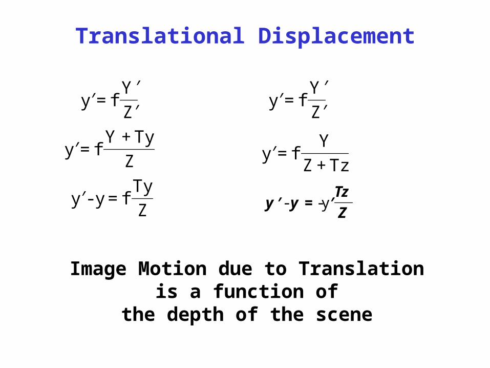
Translational Displacement
Z′Y′
f=y′
Z
Ty+Yf=y′
Z
Tyf=y-y′
Z′Y′
f=y′
Tz+Z
Yf=y′
Z
Tzyy y-- ′=′
Image Motion due to Translationis a function of
the depth of the scene


Sample Displacement Fields
Render scenes with various motions and plot the displacement fields

Motion Field vs. Optical Flow
X
Y
Z
Tx
Ty
Tz
wx
wy
wz
P
pP’p’
Motion Field : 2D projections of 3Ddisplacement vectors due to camera and/or object motion
Optical Flow : Image displacement fieldthat measures the apparent motion ofbrightness patterns

Motion Field vs. Optical Flow
Lambertian ball rotating in 3D
Motion Field ?
Optical Flow ?
Courtesy : Michael Black @ Brown.eduImage: http://www.evl.uic.edu/aej/488/

Motion Field vs. Optical Flow
Stationary Lambertian ball with amoving point light source
Motion Field ?
Optical Flow ?
Courtesy : Michael Black @ Brown.eduImage : http://www.evl.uic.edu/aej/488/

• Parametric motion models – 2D translation, affine, projective, 3D pose [Bergen, Anandan, et.al.’92]
• Piecewise parametric motion models– 2D parametric motion/structure layers [Wang&Adelson’93, Ayer&Sawhney’95]
• Quasi-parametric– 3D R, T & depth per pixel. [Hanna&Okumoto’91]
– Plane+parallax [Kumar et.al.’94, Sawhney’94]
• Piecewise quasi-parametric motion models– 2D parametric layers + parallax per layer [Baker et al.’98]
• Non-parametric– Optic flow: 2D vector per pixel [Lucas&Kanade’81, Bergen,Anandan et.al.’92]
A Hierarchy of Models
Taxonomy by Bergen,Anandan et al.’92

Sparse/Discrete Correspondences
&
Dense Motion Estimation

Discrete Methods
Feature Correlation&
RANSAC

Visual Motion through Discrete Correspondences
pp′
Images may be separated by time, space, sensor types
In general, discrete correspondences are related
through a transformation

Discrete Methods
Feature Correlation&
RANSAC

Discrete Correspondences
• Select corner-like points• Match patches using Normalized Correlation• Establish further matches using motion model

Direct Methods for Visual Motion Estimation
Employ Models of Motionand
Estimate Visual Motionthrough
Image Alignment

Characterizing Direct MethodsThe What
• Visual interpretation/modeling involves spatio-temporal image representations directly– Not explicitly represented discrete features like
corners, edges and lines etc.
• Spatio-temporal images are represented as outputs of symmetric or oriented filters.
• The output representations are typically dense, that is every pixel is explained,– Optical flow, depth maps.– Model parameters are also computed.
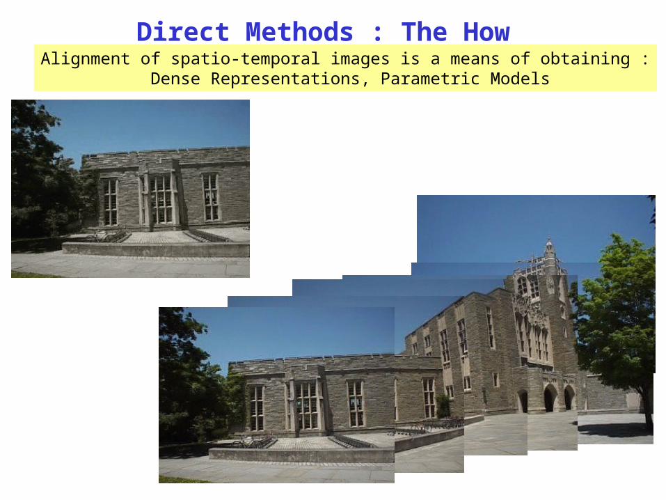
Direct Methods : The How Alignment of spatio-temporal images is a means of obtaining :
Dense Representations, Parametric Models

Direct Method based Alignment

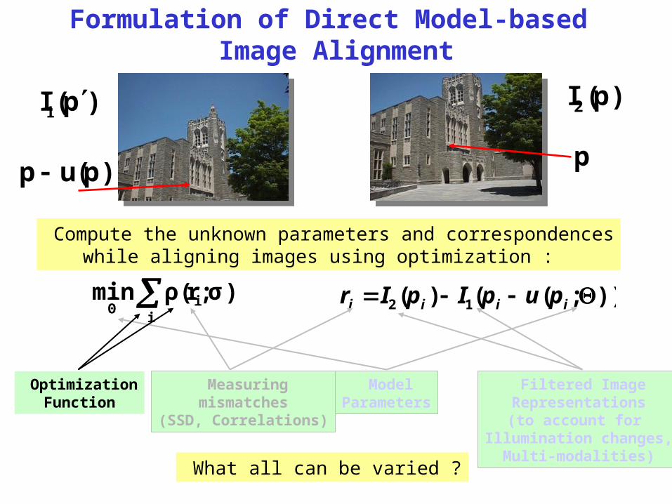
Formulation of Direct Model-based Image Alignment[Bergen,Anandan et al.’92]
)p(I1 )p(I2
p)p(up
Model image transformation as :
)());(()( 112 pIpupIpI
Images separated by
time, space, sensor types
BrightnessConstancy

Formulation of Direct Model-based Image Alignment
)p(I1 )p(I2
p)p(up
Model image transformation as :
))Θ;p(up(I)p(I 12
Images separated by
time, space, sensor types
Reference Coordinate
System

Formulation of Direct Model-based Image Alignment
)p(I1 )p(I2
p)p(up
Model image transformation as :
))Θ;p(up(I)p(I 12
Images separated by
time, space, sensor types
Reference Coordinate
System
Generalized pixel
Displacement

Formulation of Direct Model-based Image Alignment
)p(I1 )p(I2
p)p(up
Model image transformation as :
))Θ;p(up(I)p(I 12
Images separated by
time, space, sensor types
Reference Coordinate
System
Generalized pixel
Displacement
ModelParameters

Formulation of Direct Model-based Image Alignment
)p(I1 )p(I2
p)p(up
Model image transformation as :
))Θ;p(up(I)p(I 12
Images separated by
time, space, sensor types
Reference Coordinate
System
Generalized pixel
Displacement
ModelParameters
Formulation of Direct Model-based Image Alignment
)p(I1 )p(I2
p)p(up
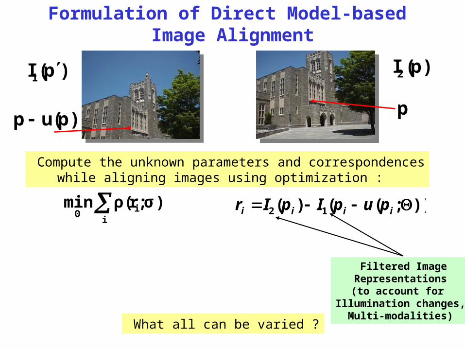
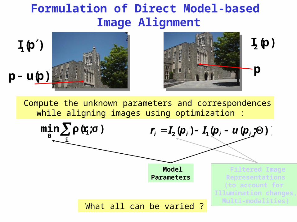
Compute the unknown parameters and correspondenceswhile aligning images using optimization :
i
iΘ
),σ;r(ρmin ));(()( 12 iiii pupIpIr
What all can be varied ?
Filtered ImageRepresentations(to account for
Illumination changes,Multi-modalities)
Formulation of Direct Model-based Image Alignment
)p(I1 )p(I2
p)p(up
Compute the unknown parameters and correspondenceswhile aligning images using optimization :
i
iΘ
),σ;r(ρmin ));(()( 12 iiii pupIpIr
What all can be varied ?
Filtered ImageRepresentations(to account for
Illumination changes,Multi-modalities)
ModelParameters
Measuringmismatches
(SSD, Correlations)
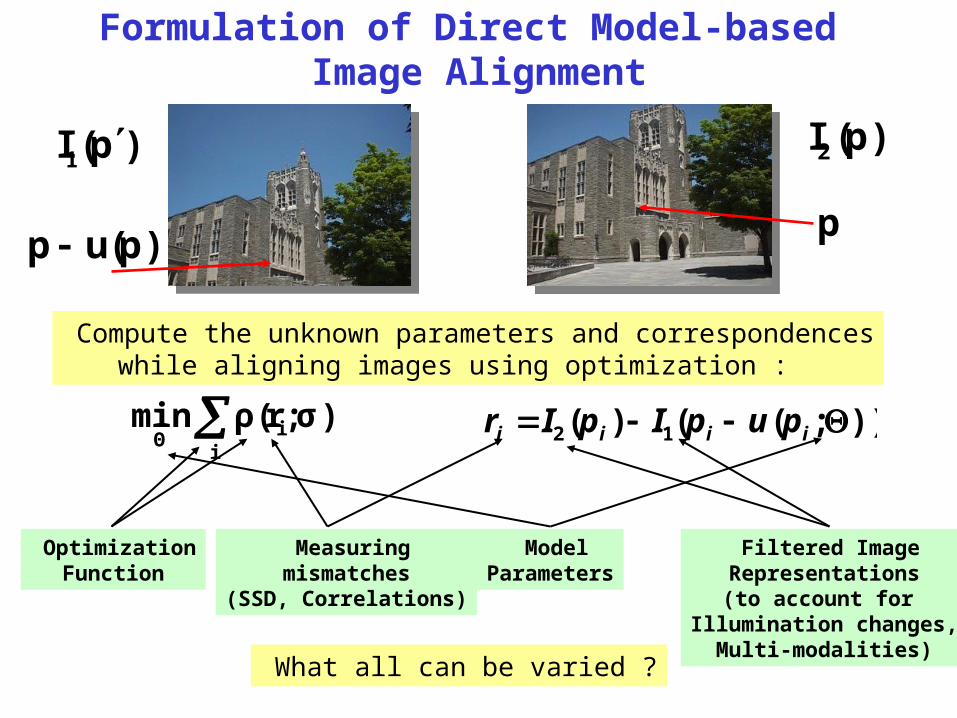
OptimizationFunction

• Parametric motion models – 2D translation, affine, projective, 3D pose [Bergen, Anandan, et.al.’92]
• Piecewise parametric motion models– 2D parametric motion/structure layers [Wang&Adelson’93, Ayer&Sawhney’95]
• Quasi-parametric– 3D R, T & depth per pixel. [Hanna&Okumoto’91]
– Plane+parallax [Kumar et.al.’94, Sawhney’94]
• Piecewise quasi-parametric motion models– 2D parametric layers + parallax per layer [Baker et al.’98]
• Non-parametric– Optic flow: 2D vector per pixel [Lucas&Kanade’81, Bergen,Anandan et.al.’92]
A Hierarchy of Models
Taxonomy by Bergen,Anandan et al.’92

Plan : This Part
• First present the generic normal equations.
• Then specialize these for a projective transformation.
• Sidebar into backward image warping.
• SSD and M-estimators.

An Iterative Solution of Model Parameters
[Black&Anandan’94 Sawhney’95]
i
iΘ
),σ;r(ρmin ));(()( 12 iiii pupIpIr
• Given a solution )m(Θ at the mth iteration, find Θδ by solving :
l i i k
ii
i
il
l
i
k
i
i
i rr
r
rrr
r
r
)()(
k
iw
• iw is a weight associated with each measurement.

An Iterative Solution of Model Parameters
i
iΘ
),σ;r(ρmin ));(()( 12 iiii pupIpIr
• In particular for Sum-of-Square Differences :
l i i k
iil
l
i
k
i rr
rr
k
2
2
2 r
SSD
• We obtain the standard normal equations:
• Other functions can be used for robust M-estimation…
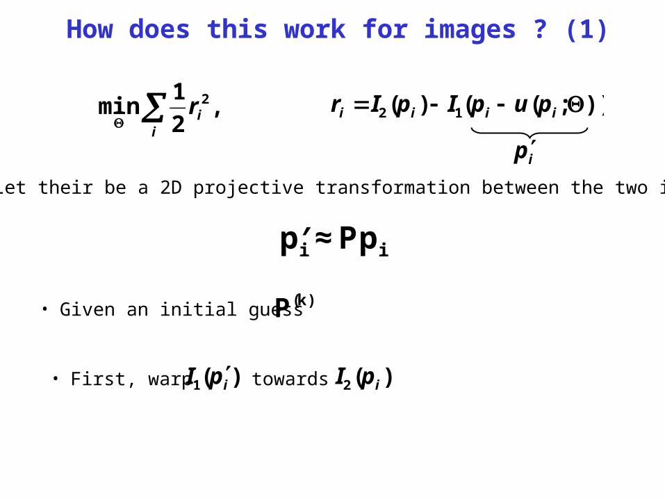
How does this work for images ? (1)
i
ir ,2
1min 2 ));(()( 12 iiii pupIpIr
ip
• First, warp
• Given an initial guess)k(Ρ
)(1 ipI towards )(2 ipI
• Let their be a 2D projective transformation between the two images:
ii pp Ρ≈′

How does this work for images ? (2)
i
ir ,2
1min 2 ));(()( 12 iiii pupIpIr
ip
( ) )p(ΡI)p(I)(pI wk11
ww1 =′=
)p(I1 )p(I2
p)p(up
)(pI ww1
( ) wk pΡ

How does this work for images ? (3)
i
ir ,2
1min 2 ));(()( 12 iiii pupIpIr
ip( ) )p(ΡI)p(I)(pI wk11
ww1 =′=
)p(I1 )p(I2
p)p(up
)(pI ww1
( ) wk pΡ
:)(pI ww1
Represents image 1 warped towards the reference image 2,Using the current set of parameters

How does this work for images ? (4)
• The residual transformation between the warped image and the reference image is modeled as:
));p(pp(I)p(Ir iiiw
1i2i Θδδ= www --
Wherei
wi D]p[Ip +≈
=
032d31d
23d22d21d
13d12d11d
D

How does this work for images ? (5)
• The residual transformation between the warped image and the reference image is modeled as:
))D;p(pp(I)p(I=r iiiw
1i2iwww -- δ
d|d
pI;0))(p(pI)(pI 0D
wiw
iw
iw
i2
T
=∂
∂∇--≈
1ydxd
d)yd(1xd1ydxd
dyd)xd(1
p
3231
232221
3231
131211
w
2
2
0D
w
yxy1yx000
xyx0001yx|
D
p

How does this work for images ? (6)
)I(p-∇∇≈r ii δ= d|pI 0D
wiD
wi
T
i
ir ,2
1min 2
)I(p∇∇∇ ∇∇ iii
∑∑ δ= wi
TD
wiD
wi
wi
wi
TD pdpIIp
TT
gHd =
D][IΡΡ (k)1)(k
So now we can solve for the model parameters while aligning images iteratively using warping and Levenberg-Marquat style optimization

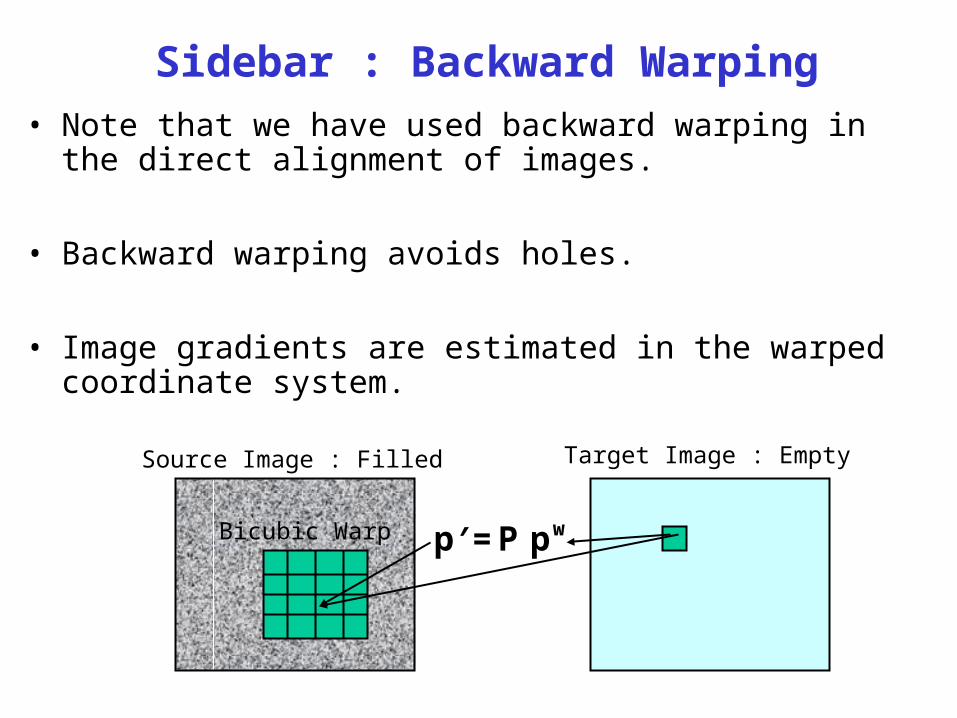
Sidebar : Backward Warping• Note that we have used backward warping in the direct
alignment of images.
• Backward warping avoids holes.
• Image gradients are estimated in the warped coordinate system.
Target Image : EmptySource Image : Filled
wpΡp =′Bilinear Warp
Sidebar : Backward Warping• Note that we have used backward warping in the direct
alignment of images.
• Backward warping avoids holes.
• Image gradients are estimated in the warped coordinate system.
Target Image : EmptySource Image : Filled
wpΡp =′Bicubic Warp

delay
estimateglobal shift
warp
)(tI
)1(ˆ tI
)(td
)(td
I (t 1)
Iterative Alignment : Result

How to handle Large Transformations ?
[Burt,Adelson’81]
• A hierarchical framework for fast algorithms
• A wavelet representation for compression, enhancement, fusion
• A model of human vision
Gaussian
Laplacian
PyramidProcessing

Iterative Coarse-to-fine Model-based Image Alignment Primer
p
2
ΘΘ))u(p;(pI(p)I( 21min )
{ R, T, d(p) }{ H, e, k(p) }
{ dx(p), dy(p) }
d(p)
Warper -

• Coarse levels reduce search.
• Models of image motion reduce modeling complexity.
• Image warping allows model estimation without discrete feature extraction.
• Model parameters are estimated using iterative non-linear optimization.
• Coarse level parameters guide optimization at finer levels.
Pyramid-based Direct Image Alignment Primer

Application : Image/Video Mosaicing
• Direct frame-to-frame image alignment.
• Select frames to reduce the number of frames & overlap.
• Warp aligned images to a reference coordinate system.
• Create a single mosaic image.
• Assumes a parametric motion model.

Princeton Chapel Video Sequence54 frames
Video Mosaic ExampleVideoBrush’96

Unblended Chapel Mosaic

• Chips are images.
• May or may not be captured from known locations of the camera.
Image Mosaics

Output Mosaic

Handling Moving Objects in 2D Parametric Alignment &
Mosaicing

Generalized M-Estimation
i
iΘ
),σ;r(ρmin ));(()( 12 iiii pupIpIr
• Given a solution )m(Θ at the mth iteration, find Θδ by solving :
l i i k
ii
i
il
l
i
k
i
i
i rr
r
rrr
r
r
)()(
k
iw
• iw is a weight associated with each measurement.Can be varied to provide robustness to outliers.
Choices of the );r( i σρ function:
2SS
σ
1
r
)r(ρ
222
2GM
)rσ(
σ2
r
)r(ρ
2
2
SS σ2
rρ
22
22
GM σr1
σrρ

Optimization Functions & their Corresponding Weight Plots
Geman-Mclure Sum-of-squares
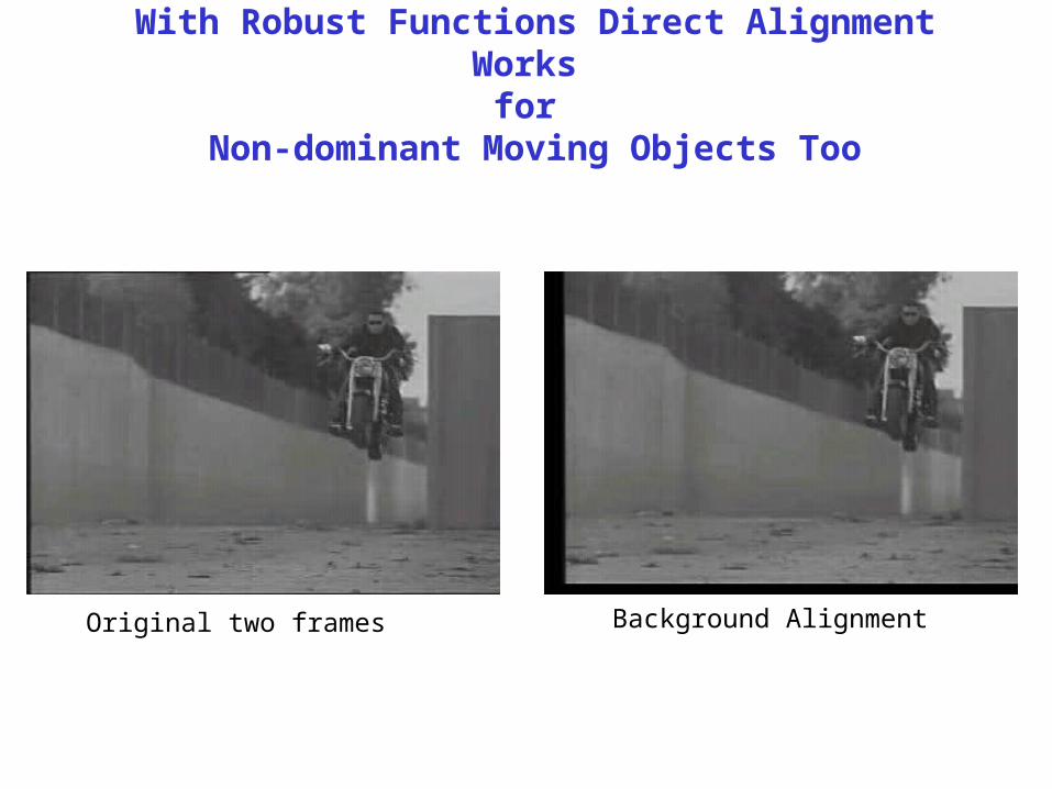
With Robust Functions Direct Alignment Works
for Non-dominant Moving Objects Too
Original two frames Background Alignment

Object Deletion with Layers
Video Stream with deleted moving objectOriginal Video

Optic Flow Estimation
))D;p(pp(I)p(I=r iiiw
1i2iwww -- δ
pI;0))(p(pI)(pITw
iw
iw
i2 δ∇--≈
[ ] I)(pI)(pIy
xII w
iw
i2wy
wx δ
δ
δ=≈ -
Gradient Direction Flow Vector

Normal Flow ConstraintAt a single pixel, brightness constraint:
0IvIuI tyx =++
Normal FlowI
I- t
∇


Computing Optical Flow:Discretization
• Look at some neighborhood N:
0
0),(),(
want
want
N),(
T
bAv
v jiIjiIji
t
0
0),(),(
want
want
N),(
T
bAv
v jiIjiIji
t
),(
),(
),(
),(
),(
),(
22
11
22
11
nnt
t
t
nn jiI
jiI
jiI
jiI
jiI
jiI
bA
),(
),(
),(
),(
),(
),(
22
11
22
11
nnt
t
t
nn jiI
jiI
jiI
jiI
jiI
jiI
bA

Computing Optical Flow:Least Squares
• In general, overconstrained linear system
• Solve by least squares
bAAAv
bAvAA
bAv
T1T
TT
want
)(
)(
0
bAAAv
bAvAA
bAv
T1T
TT
want
)(
)(
0

Computing Optical Flow:Stability
• Has a solution unless C = ATA is singular
Ny
Nyx
Nyx
Nx
nn
nn
III
III
jiI
jiI
jiI
jiIjiIjiI
2
2
22
11
2211
T
),(
),(
),(
),(),(),(
C
C
AAC
Ny
Nyx
Nyx
Nx
nn
nn
III
III
jiI
jiI
jiI
jiIjiIjiI
2
2
22
11
2211
T
),(
),(
),(
),(),(),(
C
C
AAC

Computing Optical Flow:Stability
• Where have we encountered C before?• Corner detector!• C is singular if constant intensity or edge• Use eigenvalues of C:
– to evaluate stability of optical flow computation– to find good places to compute optical flow
(finding good features to track)– [Shi-Tomasi]

Example of Flow Computation

Example of Flow Computation

Example of Flow Computation
But this in general is not the motion field

Motion Field = Optical Flow ?
From brightness constancy, normal flow:E
E-
E
v)E(v t
T
n ∇∇∇
==
Motion field for a Lambertian scene:
E
)xn(Iv
T
∇=∴
ωρΔ
nIE Tρ= )xn(IEvE Tt
T ωρ=+∇xnω=dt
dn
Points with high spatial gradient are the locationsAt which the motion field can be best estimated
By brightness constancy (the optical flow)

Motion Illusions in
Human Vision

Aperture Problem
• Too big:confused bymultiple motions
• Too small:only get motionperpendicularto edge

Ouchi Illusion
The Ouchi illusion, illustrated above, is an illusion named after its inventor,
Japanese artist Hajime Ouchi. In this illusion, the central disk seems to float above the checkered background when
moving the eyes around while viewing the figure. Scrolling the image horizontally or vertically give a much stronger effect.
The illusion is caused by random eye movements, which are independent in the horizontal and vertical directions.
However, the two types of patterns in the figure nearly eliminate the effect of the eye movements parallel to each type
of pattern. Consequently, the neurons stimulated by the disk convey the signal that the disk jitters due to the horizontal
component of the eye movements, while the neurons stimulated by the background convey the signal that movements
are due to the independent vertical component. Since the two regions jitter independently, the brain interprets the regions
as corresponding to separate independent objects (Olveczky et al. 2003).
http://mathworld.wolfram.com/OuchiIllusion.html

Akisha Kitakao
http://www.ritsumei.ac.jp/~akitaoka/saishin-e.html

Rotating Snakes
