Viscoelastic Behaviour of Pumpkin Balloons

T. Gerngross, Y. Xu and S. Pellegrino ∗Department of Engineering, University of Cambridge

Trumpington Street, Cambridge, CB2 1PZ, UK

Abstract

The lobes of the NASA ULDB pumpkin-shaped super-pressure balloons are madeof a thin polymeric film that shows considerable time-dependent behaviour. A non-linear viscoelastic model based on experimental measurements has been recentlyestablished for this film. This paper presents a simulation of the viscoelastic be-haviour of ULDB balloons with the finite element software ABAQUS. First, thestandard viscoelastic modelling capabilities available in ABAQUS are examined,but are found of limited accuracy even for the case of simple uniaxial creep tests onULDB films. Then, a nonlinear viscoelastic constitutive model is implemented bymeans of a user-defined subroutine. This approach is verified by means of biaxialcreep experiments on pressurized cylinders and is found to be accurate provided thatthe film anisotropy is also included in the model. A preliminary set of predictions fora single lobe of a ULDB is presented at the end of the paper. It indicates that time-dependent effects in a balloon structure can lead to significant stress redistributionand large increases in the transverse strains in the lobes.

Key words: atmospheric balloons, viscoelasticity, creep, polyethylene film,Schapery

1 Introduction

The NASA Ultra Long Duration Balloon (ULDB) project is developing bal-loon structures with diameters of up to 120 m. ULDB designs involve over200 identical gores made of a thin polymeric film attached to high stiffness,meridional tendons. While the behaviour of the tendons is essentially time-independent, the film shows considerable viscoelastic behaviour.

∗ Corresponding author.Email address: sp28@cam.ac.uk (S. Pellegrino).

Preprint submitted to Elsevier Science 31 March 2007

Thin polymeric films have been used in atmospheric balloons for many yearsand their viscoelastic behaviour has been studied extensively. Of particularrelevance to the present study is a description of the ULDB film material byRand and co-workers (Henderson, Caldron and Rand, 1994; Rand, Grant andStrganac, 1996; Rand, Henderson and Grant, 1996) that is based on Schapery’sclassical work (Schapery, 1969). In this paper, this formulation will be denotedas the Schapery-Rand model. An alternative model, based on a decompositioninto thermodynamically derived functions, instead of the master curve used inthe Schapery model, has been proposed by Vialettes et al. (2005) in connectionwith CNES super-pressure balloons.

This paper uses a User-Defined Material (UMAT) subroutine in the commer-cial finite-element software ABAQUS to study the time variation of the strainand stress distribution in a pumpkin balloon. Detailed predictions from thisapproach are compared to photogrammetry measurements on simple balloonsof cylindrical shape. Preliminary results for the behaviour of a 10 m diame-ter pumpkin balloon with 145 lobes are obtained, also with ABAQUS, usinga simple power-law creep model. These results indicate that time-dependenteffects in a balloon structure can lead to a significant stress redistribution andlarge increases in the transverse strains in the lobes.

The paper is set out as follows. First, in the next section, the Schapery-Randmodel is outlined and the numerical parameters are defined for the case of theULDB film. Next, in Section 3, the standard viscoelastic modelling capabilitiesavailable in ABAQUS are investigated for uniaxial test cases. It is shownthat the built-in viscoelastic models give reasonable results, but not a fullyaccurate fit to experimental data. It is also found that analytical predictionsfrom the Schapery-Rand model are much more accurate. Section 4 outlinesa user-defined material subroutine in ABAQUS, whose performance is thentested for uniform biaxial creep in two cylinder tests. The numerical resultsare compared to experimental creep strain data. Finally, in Section 6, simplepredictions of the creep strains and stresses in a pumpkin balloon, based onthe ABAQUS power-law creep model are presented. Section 7 concludes thepaper.

2 Nonlinear Viscoelastic Model

2.1 Schapery-Rand Model

Schapery (1969) proposed a nonlinear viscoelastic constitutive model wherethe transient material behavior is defined by a function known as the mastercurve. This is a plot of creep compliance, D, additional to the instantaneous

2

compliance, D0, in terms of a time variable ψ, known as the reduced time. Non-linearities are captured by including four functions of stress and temperature.The dependence of reduced time on temperature is captured by an additionalfunction, of temperature only.

More precisely, the reduced time is defined as

ψ(t) =∫ t

0

dτ

aT (T )aσ(T, σ)(1)

where aT is a temperature dependent function and aσ a stress and temperaturedependent function.

Then, the total uniaxial strain is obtained from:

ε(t) = g0D0σ(t) + g1

∫ t

0(D(ψ(t)− ψ(τ))

d(g2σ(τ))

dτdτ (2)

where the first term represents the instantaneous, i.e. elastic response while thesecond term describes the transient response. Note the nonlinearity factors: g0

is the change of instantaneous elastic compliance, g1 is the change of transientcompliance, and g2 is the sensitivity to transient stress. They are all functionsof stress and temperature.

Rand, Grant and Strganac (1996) extended Schapery’s uniaxial formulationto the case of plane stress. The nonlinearity functions were related to a singleeffective stress σ̄ given, at any time t, by

σ̄ =√

σ21 + 2A12σ1σ2 + A22σ2

2 + A66σ212 (3)

where σ1, σ2 are the normal stress components in the machine and transversedirections of the film, respectively, and σ12 is the shear stress. The coefficientsAij are chosen such that the nonlinearity functions for the machine directioncan be used to determine the nonlinearities in any direction.

2.2 ULDB Film Parameters

A material that has been used extensively for stratospheric balloons is a LinearLow Density Polyethylene (LLDPE) called StratoFilm 372, or SF372. Exper-imental data for this material has been published (Henderson, Caldron andRand, 1994; Rand, Grant and Strganac, 1996; Rand, Henderson and Grant,1996). More recently, a film called StratoFilm 420 has been introduced, whichis a three layer extrusion from the same resin as SF372, with a total thicknessof 0.038 mm. The material used for the experiments presented in this paperwas SF430; this is essentially the same as SF420, but without an additive for

3

-10 -8 -6 -4 -2 0 2 4- 9.8

-9.4

-9.0

- 8.6

-8.2

Log ψ [s]

Lo

g D

[1

/Pa

]

Fig. 1. Master curve for transient creep compliance of SF372 in machine direction,from Rand, Henderson and Grant (1996).

-40 -20 0 +2002468

10

Temperature [oC]

Log a

T

(a) aT

0 4 8 12 16 20 24

-1.2

-0.8

-0.4

0.0

Stress [MPa]

Log

aσ

23oC

0oC

-30oC-50oC

(b) aσ

0 5 10 15 20 250.41.01.41.82.22.6

Stress [MPa]

g2

23oC0oC

-30oC-50oC

(c) g2

Fig. 2. Nonlinearity functions for SF372, from Rand, Henderson and Grant (1996).

protection from ultraviolet light. After some initial uniaxial creep experimentson SF430, it was decided that it would be reasonable to use the material datafor SF372.

Figures 1 and 2 show the viscoelastic material data in the machine directionfor SF372. The data presented includes the master curve, the temperatureshift function aT , and the nonlinearity functions aσ and g2. The nonlinearityparameters g0 and g1 in the general Schapery model, Equation (2), are setequal to 1.0. Note that the master curve relates to a temperature of 23◦C.The instantaneous elastic compliance D0 = 3×10−10 Pa−1 has been estimatedat the smallest ψ available, ψ ≈ 10−10 s. The coefficients of Equation (3) arelisted in Table 1, for plane stress at 23◦C.

Table 1Biaxial stress coefficients for SF372 at 23◦C

A12 A22 A66

-1.08 1.18 6.05

4

3 Viscoelastic Capabilities in ABAQUS

3.1 Power Law Creep Option

The finite element package ABAQUS offers a power-law model that can beused in time hardening or strain hardening form, via the ∗creep function.Both forms define an equivalent uniaxial creep strain rate that depends onthe equivalent uniaxial deviatoric stress, the total time, and three user-definedfunctions of temperature. The time hardening form is expressed as

˙̄εcr

= Aσ̄ntm (4)

Assuming constant uniaxial stress σ̄0 and constant temperature, integrationof Equation (4) yields

ε̄cr =A

m + 1σ̄n

0 tm+1 (5)

The parameters A, n, m can be obtained by fitting Equation (5) to the LLDPEmaster curve, Figure 1, but this requires that one particular value of σ̄0 beassumed.

This approach is found to be quite accurate at or near the particular stressat which the model was fitted to the experimental data, however there can besignificant errors at other stress levels. For example, Figure 3 shows (amongother results) the power-law model predictions obtained for a uniaxial stressof 4 MPa using a model fitted to experimental data at σ̄0 = 2 MPa. Thecoefficients of the model are listed in Table 2.

Table 2Coefficients for power-law fit (T = 20◦C, σ̄0 = 2 MPa)

A n m

1.82× 10−4 1.63 -0.925

3.2 Shear Test Data Option

Another possibility is to use the ∗viscoelastic command in conjunctionwith ∗shear test data, in order to generate a viscoelastic model based onexperimental data from either creep or relaxation tests.

This approach is based on a stress relaxation formulation that assumes strainas the independent state variable. Similar to the way creep data was usedin Equation (2), stress relaxation can be written as (McCrum, Buckley and

5

Bucknall, 2003)

σ =∫ t

0E(t− τ)

dε(τ)

dτdτ (6)

where E(t) is the tensile stress relaxation modulus at time t. The ABAQUSformulation uses normalised shear test data, and hence Equation (6) needs tobe rewritten as (ABAQUS, 2003):

τ(t) = G0

∫ t

0gR(t− τ)

dγ(τ)

dτdτ (7)

where γ is the shear strain and gR(t) is the normalised shear relaxation mod-ulus, defined as gR(t) = GR(t)/G0. Here GR(t) is the time-dependent shearrelaxation modulus and G0 = GR(0) is the instantaneous shear modulus.

The normalised relaxation modulus is defined by a sum of exponentials knownas a Prony series, and can be written as:

gR(t) = 1−N∑

i=1

gi

(1− e

− tτi

)(8)

ABAQUS will compute the terms in the Prony series automatically from agiven set of normalized shear creep compliance data, which can be derived byadding the instantaneous compliance to the master curve data and dividingby the instantaneous compliance. The Poisson’s ratio of the film is assumedto remain unchanged over time, and hence does not appear in the normalizedshear compliance.

This method is a linear version of Schapery’s constitutive equation, as can beseen by comparing Equation (2) with Equation (6). However, stress dependentnonlinearities are, again, not captured by this approach.

When the master curve in Figure 1 was entered as creep test data spanning16 decades of time, ABAQUS encountered problems with the automatic con-version to a Prony series. To overcome this problem the creep data was trans-formed into relaxation data and then the automatic conversion to a Pronyseries worked fine.

3.3 Validation

Predictions from the two different viscoelastic options in ABAQUS were com-pared to a direct solution of the Schapery-Rand nonlinear viscoelastic modelwith the parameters defined in Section 2, and also to experimental measure-ments. As already mentioned, the parameters for the ABAQUS models wereobtained by fitting to experimental data at a constant stress of 2 MPa. The

6

accuracy of the models was tested by simulating the creep response of a uni-axial specimen subject to a constant stress of 2 MPa and it was found thatvery good agreement could be achieved with the ∗viscoelastic option, bymodifying the slope of the function g2 values for 23◦C, in Figure 2(c). Theresults obtained with the ∗creep option were less good.

A validation exercise was then carried out for uniaxial creep tests at a constantstress level of 4 MPa, to assess the accuracy of stress-independent creep modelsfor SF372. The results are shown in Figure 3.

0

1

2

3

4

0 1000 2000 3000 4000 5000

Time [s]

Tota

l str

ain

[%

]

*creep

*viscoelastic

Rand-Schapery

experiment

Fig. 3. Comparison of viscoelastic models at stress of 4 MPa.

Both ABAQUS options give rather poor results, the power-law model basedon the ∗creep option predicts strains up to 10% lower. The ∗viscoelasticoption, which follows the linear Schapery viscoelastic constitutive equation,but similarly neglects the stress dependent nonlinearities of the material, un-derpredicts the creep strains by up to 40%.

On the other hand, the creep strains predicted by the Schapery-Rand modelpractically coincide with the experimental data. The next section describesan implementation of this model in ABAQUS in the form of a user definedmaterial.

4 ABAQUS UMAT Subroutine

To implement the Schapery-Rand constitutive model in a numerical algo-rithm, Equation (2) needs to be rewritten in incremental form. A numericalintegration method for a three-dimensional, isotropic, viscoelastic materialhas been presented by Haj-Ali and Muliana (2004). Following the same ap-proach, during the present study the Schapery-Rand model was implemented

7

in ABAQUS. The present work could be readily extended to any displace-ment based finite element software, where the strain components are used asindependent state variables.

The viscoelastic properties are entered as material constants in the ABAQUSinput file ∗user material. The incremental formulation requires the transientcompliance D to be expressed in terms of a Prony series, as in Section 3.2. 16terms were included.

A graphical depiction of the algorithm is shown in Figure 4. ABAQUS callsUMAT during each increment and for each integration point. The ABAQUSinterface for a user defined material passes a time increment ∆t and a corre-sponding strain increment ∆εABAQUS, this is determined using the Jacobianmatrix computed at the end of the previous time increment.

Every time UMAT is called it starts with an estimation of a trial stress incre-ment, ∆σtrial, based on the nonlinearity parameters at the end of the previoustime increment. With this initial guess an iterative loop is entered, where in-tegration of Equation (2) yields a trial strain increment, ∆εtrial, which is thencompared with ∆εABAQUS. If required, the trial stresses and the nonlinearityparameters are corrected and the loop is repeated. Alternatively, if the strainerror residual is below a tolerance (set to tol = 10−7) UMAT exits the loop

and updates the Jacobian matrix ∂∆σj

∂∆εiand the stresses σj. Also, at the end of

the increment the history for every strain/stress component and every Pronyterm is stored using the statev array.

ABAQUS passes:

stress/strain history

∆εABAQUS, ∆t

trial ∆σtrial

nonlinearity

parameters

∆εtrial = εt -εt-∆t

residual66

-1

[ ] x residual∆σ

stress correction =

check

residual

norm

∆εABAQUS -∆εtrialresidual =

return to ABAQUS:

Jacobian=[ ] residual6

6 ∆σ

-1stress update,

store stress/strain history

Fig. 4. Iterative algorithm in UMAT.

8

5 Verification of UMAT Subroutine

The accuracy of the nonlinear viscoelastic model implemented in the ABAQUSUMAT subroutine was verified against experimental creep strain measure-ments on two pressurized cylinders.

5.1 Experiment

The cylinders had a diameter of 300 mm and height of 760 mm, and weremade of SF430. The overall test layout can be seen in Figure 5(a).

5.1.1 Specimen Preparation and Setup

Two layers of SF430 were placed on top of each other and heat-sealed with asoldering iron. Symmetry was achieved by forming two diametrically opposite,parallel seams. End-fittings made of MDF panels were attached to the cylinderwith jubilee clamps and sealed with silicone and felt padding.

At mid-height the cylinder was fitted with nine self-adhesive coded targetsfor photogrammetry strain measurements, plus 2 targets for reference. Thetargets were located over a 40 × 40 mm square region, see Figure 5(b).

(a) Experimental setup (b) Measurementregion

Fig. 5. Cylinder specimen.

The bottom end fitting was clamped to a rigid support, while the top end

9

fitting was suspended from a string going over a pulley arrangement to acounterweight hanger, see Figure 5(a). The cylinder was attached to an air-line for pressurization and to a Sensor Technics pressure transducer with amaximum pressure of 2500 Pa.

Four Olympus SP-350 digital cameras (with a resolution of 8.0 Mpixel) wereconnected to a personal computer and mounted in front of the target area.The cameras were triggered via the computer and so produced sets of foursimultaneous photos of the coded targets, each from a different view point.

5.1.2 Procedure

Initially, the weights on the counterweight hanger were set to match the weightof the top end fitting, in order to remove any load from the cylinder.

The pressure regulator was set to the nominal experimental pressure, see Ta-ble 3. At the same time the axial load on the cylinder was increased by hangingadditional weights through the counterweight hanger. The cylinder pressurewas recorded throughout the experiment. While the increase of the counter-weight resulted in an instantaneous increment in axial loading, full pressur-ization was reached only after ∼10 seconds.

Under loading the viscoelastic film deformed and the movement of the codedtargets was recorded by taking a series of close-up photos. Photos of the mea-surement area were taken, initially at intervals of a few seconds and increasingto five minutes towards the end of the experiment. Three-dimensional coor-dinates of the targets were then computed by means of the photogrammetrysoftware Photomodeler (2004). The strain components in the axial and hoopdirections were computed from the changes of coordinates of the targets overtime.

5.2 Analysis

It was assumed that the cylinder would be under a biaxial state of stressthroughout the experiment, and so wrinkle free. This allowed the film to bemodelled with triangular membrane elements; a mesh of 72 M3D3 elementsin the hoop direction and 56 elements in the longitudinal direction was used.Wrinkling of the film, which occurs near the end-fittings, was neglected becausethe creep measurements were taken away from the ends. One end fitting wasfully constrained, whereas the other end of the cylinder was allowed to moveaxially.

A uniform internal pressure was applied, through the ∗dload command, and

10

axial forces were simultaneously applied through the ∗cload command. Bothloads were increased from zero to their final value in a single instantaneousstep and kept constant for 5100 s.

The film was assumed to be isotropic with a Poisson’s ratio of 0.49 and aconstant thickness of 0.038 mm. The analysis was run at a constant roomtemperature of 23 ◦C. Figure 6 shows the axial and hoop strains at 5100 s, incylinder 1.

+0.00

+0.45

+0.91

+1.37

+1.82

+2.28

+2.74

εhoop [%]

+0.22

+0.34

+0.47

+0.60

+0.73

+0.86

+0.98

εaxial [%]

Fig. 6. Strain distribution after 5100 s.

5.3 Comparison

Two cylinders were tested at different pressures and with different axial loads,see Table 3. Both cylinders were built with the material’s machine directionaligned with the cylinder’s hoop direction.

Table 3Cylinder experiments

Cylinder Pressure [Pa] Axial load [N]

1 930 6.28

2 1100 22.22

The total strains, i.e. including both instantaneous and time-dependent re-sponse, from experiment and analysis are compared in Figure 7. The resultsfrom the analysis based on the isotropic UMAT, with an assumed Poisson’sratio of 0.49, show a significant difference from the experimental measure-ments. Remarkably, the strain in the axial direction decreases over time in theisotropic model. This is due to anisotropy that cannot be captured with theisotropic UMAT.

11

An anisotropic version of the UMAT subroutine (which will be presented indetail elsewhere) has been implemented to establish the accuracy of a morerefined material model. In the anisotropic UMAT the hoop compliance, whichis in the machine direction of the film, was left unchanged but the longitudinalcompliance was multiplied by a factor of 0.72. Also, the Poisson’s ratios wereν12 = 0.49 and ν21 = 0.68.

The dotted lines in Figures 7(a) and 7(b) show the strains predicted by theanisotropic model; these predictions agree well with the measurements.

0 1000 2000 3000 4000 5000 6000 -0.5

0.0

0.5

1.0

1.5

2.0

2.5

3.0

Time [s]

Tota

l str

ain

[%

]

hoop

strains

axial

strains

Experiment

Isotropic UMAT

Anisotropic UMAT

(a) Pressure 930 Pa, axial load 6.28 N

-0.5

0.0

0.5

1.0

1.5

2.0

2.5

3.0

3.5

Tota

l str

ain

[%

]

0 1000 2000 3000 4000 5000 6000

Time [s]

Experiment

Isotropic UMAT

Anisotropic UMAT

hoop

strains

axial

strains

(b) Pressure 1100 Pa, axial load 22.22 N

Fig. 7. Comparison of total strains in two cylinders.

12

6 Preliminary Study of Balloon Behaviour

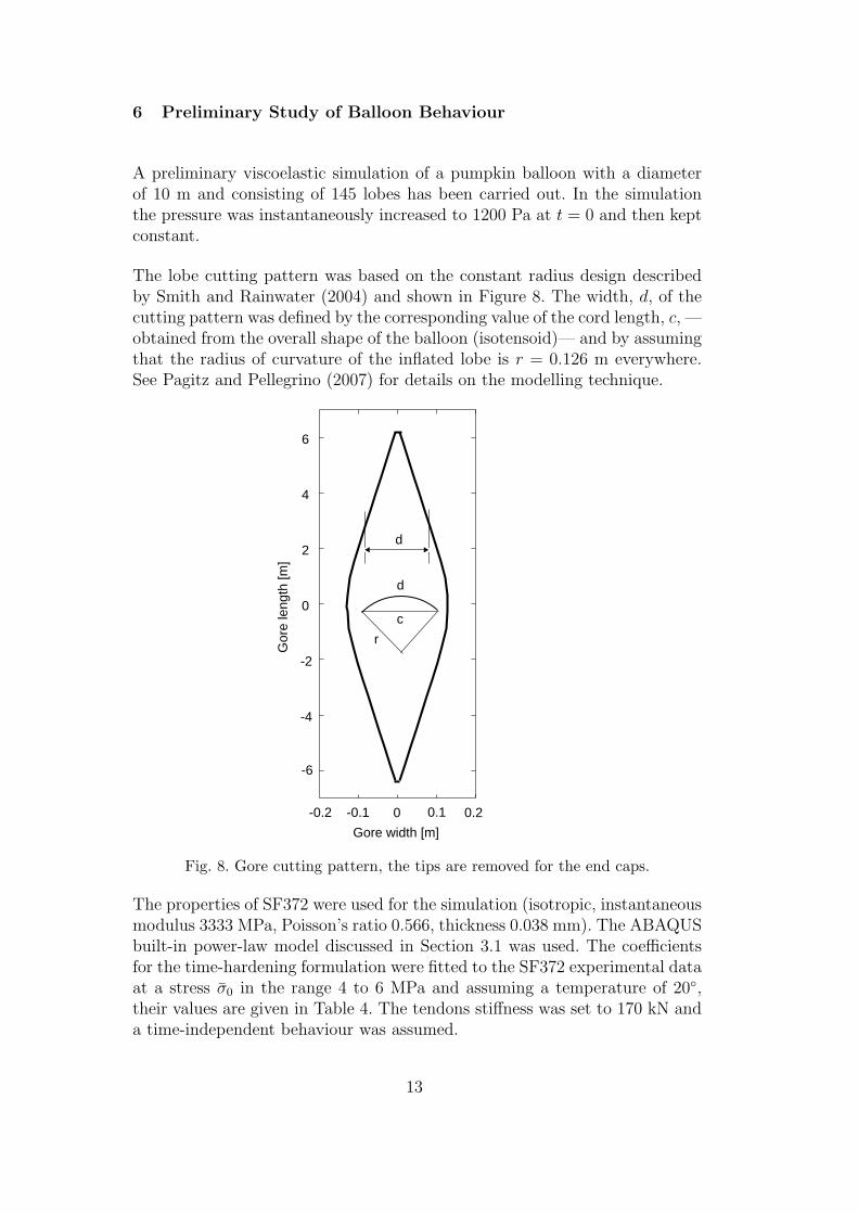
A preliminary viscoelastic simulation of a pumpkin balloon with a diameterof 10 m and consisting of 145 lobes has been carried out. In the simulationthe pressure was instantaneously increased to 1200 Pa at t = 0 and then keptconstant.

The lobe cutting pattern was based on the constant radius design describedby Smith and Rainwater (2004) and shown in Figure 8. The width, d, of thecutting pattern was defined by the corresponding value of the cord length, c, —obtained from the overall shape of the balloon (isotensoid)— and by assumingthat the radius of curvature of the inflated lobe is r = 0.126 m everywhere.See Pagitz and Pellegrino (2007) for details on the modelling technique.

-0.2 -0.1 0 0.1 0.2

-6

-4

-2

0

2

4

6

Gore width [m]

Gor

e le

ngth

[m]

d

d

r

c

Fig. 8. Gore cutting pattern, the tips are removed for the end caps.

The properties of SF372 were used for the simulation (isotropic, instantaneousmodulus 3333 MPa, Poisson’s ratio 0.566, thickness 0.038 mm). The ABAQUSbuilt-in power-law model discussed in Section 3.1 was used. The coefficientsfor the time-hardening formulation were fitted to the SF372 experimental dataat a stress σ̄0 in the range 4 to 6 MPa and assuming a temperature of 20◦,their values are given in Table 4. The tendons stiffness was set to 170 kN anda time-independent behaviour was assumed.

13

Table 4Coefficients for power-law fit (T = 20◦C)

A n m

1.27× 10−4 1.63 -0.94

The variation of strains and stresses over 1000 minutes is plotted in Figure 9.The initial strains are smaller than 0.2% both in the meridional direction andin the hoop direction. Over time, the meridional strains remain essentiallyunchanged in most of the lobe, apart from the equatorial region where theyincrease six times, whereas the hoop strains increase by a factor of about six inmost of the lobe, apart from the equatorial region where they remain approx-imately constant. The initial stress distribution has peak values of approxi-mately 8 MPa, quickly decreasing to about half this value and then remainingapproximately constant.

A simple pseudo-elastic approximation is sometimes used to predict viscoelas-tic stress distributions and for the present case Rand has estimated a pseudo-elastic modulus of 138.7 MPa. Figure 10 presents a comparison of the stressdistribution that is computed from the power-law viscoelastic model, with thatobtained from the simplified linear model. It can be seen that the linear modelproduces a roughly correct estimate of the hoop stresses, but underestimatesthe peak meridional stress.

7 Discussion and Conclusion

This paper has shown the importance of viscoelastic effects in the behaviour ofballoon structures made of LLDPE. In the particular case of ULDB balloonsour preliminary analysis results have shown that the stress distribution tendsto become more uniformly distributed, over time. This potentially importantresult will need to be verified by a more detailed analysis, of course, andtemperature effects should also be considered.

We have shown that the biaxial behaviour of the ULDB film material SF372is well modelled by the Schapery-Rand non-linear, anisotropic viscoelasticmodel. This behaviour has been captured by the anisotropic version of ourABAQUS UMAT subroutine, as shown by comparing numerical predictionsto experimental measurements taken on two cylinders. We have found that theisotropic version of the model is of limited accuracy. We have also found thatthe standard power-law creep and viscoelastic models available in ABAQUSare less accurate than the Schapery-Rand models, even in the case of prob-lems where the stress distribution is relatively uniform and it is possible todetermine the best-fit model parameters near the stress level of interest.

14

Arc-length [m]

Str

ain

[%

]

0 2 4 6 8 10 12 14

0

0.2

0.4

0.6

0.8

1.0

1.2

1.4t=0t=10 mint=100 mint=1000 min

-0.2

(a) Strain distribution

Str

ess [M

Pa]

Arc-length [m]

0 2 4 6 8 10 12 140

1

2

3

4

5

6

7

8

t=0t=10 mint=100 mint=1000 min

(b) Stress distribution

Fig. 9. Distribution of total strains and stresses along the centerline of a pumpkinballoon lobe; solid lines denote hoop strains/stresses, dotted lines denote meridionalstrains/stresses.

The ULDB film is a blown film that can be expected to show anisotropicbehaviour. This became apparent in Section 5.3 when numerical and experi-mental results were compared. While under a biaxial state of stress the higherstiffness of the material in the axial direction resulted in lower strains com-pared to the isotropic case, the axial strains were actually observed to bedecreasing. This behaviour cannot be captured by the isotropic model.

15

0 2 4 6 8 10 12 140

1

2

3

4

5

6

7

t=1000 min

Linear elastic solution

Arc-length [m]

Str

ess [M

Pa]

Fig. 10. Comparison of stress distribution obtained from pseudo-elastic simulationwith viscoelastic stress distribution after 1000 min; solid lines denote hoop stresses,dotted lines denote meridional stresses.

The discrepancy between the initial behaviour observed experimentally andthe anisotropic model predictions may be due to the rate of application of thetwo components of the loading, at the beginning of the experiment. The axialload was applied very quickly, while the nominal pressure was reached onlyafter about 10 seconds. Furthermore, a general reason for these discrepanciesmight be the use of material data describing SF372 in the analysis, while thematerial that was used with the experiment is the current ULDB materialSF430.

Acknowledgments

We thank Dr Jim Rand for advice and providing film material data to usand Dr David Wakefield for insightful suggestions. Mr Danny Ball, ColumbiaScientific Balloon Facility and Mr Loren Seely, Aerostar International haveprovided advice and materials for this study. Financial support from the NASABalloon Program Office is gratefully acknowledged.

References

Haj-Ali, R.M. and Muliana, A.H. (2004). Numerical finite element formulationof the Schapery nonlinear viscoelastic material model. International Journalfor Numerical Methods in Engineering, 59, 25–45.

16

Henderson, J.K., Caldron, G. and Rand, J.L. (1994). A nonlinear viscoelasticconstitutive model for balloon films. American Institute of Aeronautics andAstronautics AIAA-1994-638.

ABAQUS (2003). ABAQUS Version 6.3. ABAQUS, INC. 1080 Main StreetPawtucket, Rhode Island 02860-4847 USA, Pawtucket, RI 02860.

McCrum, N.G., Buckley, C.P. and Bucknall, C.B. (2003). Principles of Poly-mer Engineering, 2nd edition, Oxford Science Publications, Oxford.

Pagitz, M. and Pellegrino, S. (2007). Buckling pressure of ”pumpkin” balloons.Accepted for publication in International Journal of Solids and Structures.

Photomodeler (2004). Pro5.0 EOS Systems.Rand, J.L., Grant, D.A. and Strganac, T. (1996) The nonlinear biaxial char-

acterization of balloon film. American Institute of Aeronautics and Astro-nautics AIAA-96-0574.

Rand, J.L., Henderson, J.K. and Grant, D.A. (1996). Nonlinear behaviour oflinear low-density polyethylene. Polymer Engineering and Science, 36 (8),1058–1064.

Schapery, R.A. (1969). On the characterization of nonlinear viscoelastic ma-terials. Polymer Engineering and Science, 9 (4), 295–310.

Smith, M.S. and Rainwater, E.L. (2004). Optimum designs for superpressureballoons. Advances in Space Research, 33, 1688–1693.

Vialettes, P., Siguier, J-M., Guigue, P., Karama, M., Mistou, S., Dalverny,O., and Petitjean, F. (2005). Viscoelastic laws study for mechanical mod-elization of super-pressure balloons. American Institute of Aeronautics andAstronautics AIAA-2005-7469.

17