effective viscoelastic behaviour of cellular auxetic materials - lamp
TRANSCRIPT

Steffen Alvermann
Effective Viscoelastic Behaviour of Cellular Auxetic Materials

Monographic Series TU Graz Computation in Engineering and Science
Series Editors G. Brenn Institute of Fluid Mechanics and Heat Transfer G.A. Holzapfel Institute of Biomechanics M. Schanz Institute of Applied Mechanics W. Sextro Institute of Mechanics O. Steinbach Institute of Computational Mathematics

Monographic Series TU Graz Computation in Engineering and Science Volume 1
Steffen Alvermann _____________________________________________________ Effective Viscoelastic Behaviour of Cellular Auxetic Materials ______________________________________________________________ This work is based on the dissertation Effective Viscoelastic Behaviour of Cellular Auxetic Materials, presented by S. Alvermann at Graz University of Technology, Institute of Applied Mechanics in January 2007. Supervisor: M. Schanz (Graz University of Technology) Reviewer: M. Schanz (Graz University of Technology), G. E. Stavroulakis (Technical University of Crete)

Bibliographic information published by Die Deutsche Bibliothek. Die Deutsche Bibliothek lists this publication in the Deutsche Nationalbibliografie; detailed bibliographic data are available at http://dnb.ddb.de.
© 2008 Verlag der Technischen Universität Graz
Cover photo Vier-Spezies-Rechenmaschine
by courtesy of the Gottfried Wilhelm Leibniz Bibliothek –
Niedersächsische Landesbibliothek Hannover
Layout Wolfgang Karl, TU Graz / Universitätsbibliothek
Printed by TU Graz / Büroservice
Verlag der Technischen Universität Graz
www.ub.tugraz.at/Verlag ISBN: 978-3-902465-92-4
This work is subject to copyright. All rights are reserved, whether the whole or part of the material is concerned, specifically the rights of reprinting, translation, reproduction on microfilm and data storage and processing in data bases. For any kind of use the permission of the Verlag der Technischen Universität Graz must be obtained.

Abstract
This work is concerned with the calculation of effective, macroscopic material parametersof materials with an inhomogeneous microstructure. On the microscopic scale, the calcu-lation of a representative volume element of the material is done taking dynamical effectsinto account. This makes it possible to study damping effects on the macroscopic scale.The microstructures to be analyzed are mainly composed of trusses. They are calculatedwith a newly developed boundary element formulation, which delivers analytical exactresults. A special interest is put on microstructures which, because of their deformationmechanism, cause a negative Poisson’s ratio of a material on the macroscopic scale (aux-etic materials). The calculation of adequate macroscopic material parameters is done withdifferent optimization techniques. Beside the classical gradient-based optimization pro-cedures, also softcomputing methods like Genetic Algorithms and Neural Networks areused. A number of numerical examples are presented where effective viscoelastic materialparameters are calculated. The Genetic Algorithm turned out to deliver the most reliableresults in the homogenization process, wheras the gradient-based methods may fail due tothe existence of local minima in the optimization function.
Zusammenfassung
Die vorliegende Arbeit behandelt die Berechnung effektiver, makroskopischer Eigenschaf-ten von Materialien mit inhomogener Mikrostruktur. Auf mikroskopischer Ebene wird da-bei die Berechnung eines repräsentativen Volumenelementes des zu untersuchenden Ma-terials in der Dynamik durchgeführt, um Effekte wie beispielweise die innere Dämpfungdes makroskopischen Materials zu erfassen. Die zu untersuchenden Mikrostrukturen sindmeist einfache Balkentragwerke, die mit Hilfe einer neuentwickelten Randelementformu-lierung analytisch exakt berechnet werden. In der vorliegenden Arbeit interessieren insbe-sondere solche Strukturen, die durch ihre mikroskopische Kinematik negative Querkon-traktionszahlen auf makroskopischer Ebene verursachen (auxetische Materialien). DieBerechnung effektiver Materialparameter auf makroskopischer Ebene erfolgt mit Hilfeverschiedener Optimierungsverfahren, wobei neben klassischen Gradientenverfahren auchSoftcomputing-Methoden wie Genetische Algorithmen und Neuronale Netze zum Ein-satz kommen. Eine Reihe von Beispielrechnungen werden vorgestellt, bei denen effek-tive viskoelastische Materialparameter verschiedener Mikrostrukturen berechnet werden.Der Genetische Algorithmus liefert dabei die zuverlässigsten Ergebnisse, wohingegen dieklassischen Gradientenverfahren teilweise aufgrund lokaler Minima in der Optimierungs-funktion fehlschlagen.


CONTENTS
1 Introduction 1
2 Continuum mechanics 52.1 Kinematics of deformations . . . . . . . . . . . . . . . . . . . . . . . . . 52.2 Equilibrium . . . . . . . . . . . . . . . . . . . . . . . . . . . . . . . . . 62.3 Constitutive equation . . . . . . . . . . . . . . . . . . . . . . . . . . . . 7
2.3.1 Linear elasticity . . . . . . . . . . . . . . . . . . . . . . . . . . . 72.3.2 Linear viscoelasticity . . . . . . . . . . . . . . . . . . . . . . . . 11
2.4 Auxetic Materials . . . . . . . . . . . . . . . . . . . . . . . . . . . . . . 162.4.1 The term auxetic . . . . . . . . . . . . . . . . . . . . . . . . . . 162.4.2 Origin of auxetic behavior . . . . . . . . . . . . . . . . . . . . . 172.4.3 Naturally occurring materials . . . . . . . . . . . . . . . . . . . 182.4.4 Man-made auxetic materials and structures . . . . . . . . . . . . 182.4.5 Industrial applications . . . . . . . . . . . . . . . . . . . . . . . 20
3 Calculation of Truss Structures 233.1 Basic Equations and Fundamental Solutions . . . . . . . . . . . . . . . . 23
3.1.1 Beam . . . . . . . . . . . . . . . . . . . . . . . . . . . . . . . . 233.1.2 Bar . . . . . . . . . . . . . . . . . . . . . . . . . . . . . . . . . 27
3.2 Integral Equation . . . . . . . . . . . . . . . . . . . . . . . . . . . . . . 283.3 Boundary (Element) Equations by Collocation . . . . . . . . . . . . . . . 293.4 Assembling of System Matrix . . . . . . . . . . . . . . . . . . . . . . . 30
3.4.1 Global Coordinates . . . . . . . . . . . . . . . . . . . . . . . . . 303.4.2 Assembling . . . . . . . . . . . . . . . . . . . . . . . . . . . . . 323.4.3 Boundary Conditions . . . . . . . . . . . . . . . . . . . . . . . . 323.4.4 Transition Conditions . . . . . . . . . . . . . . . . . . . . . . . . 333.4.5 Combined Transition/Boundary Conditions . . . . . . . . . . . . 343.4.6 Solving the System Matrix . . . . . . . . . . . . . . . . . . . . . 353.4.7 Example Calculation . . . . . . . . . . . . . . . . . . . . . . . . 37
4 Micromechanics and Homogenization 414.1 Representative Volume Element . . . . . . . . . . . . . . . . . . . . . . 414.2 Classical homogenization approaches . . . . . . . . . . . . . . . . . . . 43
4.2.1 Voigt - Reuss bounds . . . . . . . . . . . . . . . . . . . . . . . . 434.2.2 Hashin - Shtrikman bounds . . . . . . . . . . . . . . . . . . . . . 454.2.3 Strain energy based homogenization . . . . . . . . . . . . . . . . 454.2.4 Surface average based approach . . . . . . . . . . . . . . . . . . 46
i

4.2.5 Unit Cell versus RVE . . . . . . . . . . . . . . . . . . . . . . . . 50
5 Optimization 535.1 Simplex Algorithm . . . . . . . . . . . . . . . . . . . . . . . . . . . . . 535.2 SQP - Sequential Quadratic Programming . . . . . . . . . . . . . . . . . 53
5.2.1 Local Minima . . . . . . . . . . . . . . . . . . . . . . . . . . . . 555.3 Genetic Algorithm . . . . . . . . . . . . . . . . . . . . . . . . . . . . . 555.4 Neural Network . . . . . . . . . . . . . . . . . . . . . . . . . . . . . . . 59
6 Effective properties in statics 636.1 Beam-type microstructures . . . . . . . . . . . . . . . . . . . . . . . . . 636.2 Plane stress microstructure . . . . . . . . . . . . . . . . . . . . . . . . . 72
7 Effective properties in dynamics 777.1 Beam cells in small frequency range . . . . . . . . . . . . . . . . . . . . 78
7.1.1 Genetic Algorithm . . . . . . . . . . . . . . . . . . . . . . . . . 797.1.2 Simplex Algorithm . . . . . . . . . . . . . . . . . . . . . . . . . 807.1.3 SQP - Sequential Quadratic Programming . . . . . . . . . . . . . 827.1.4 Discussion of results . . . . . . . . . . . . . . . . . . . . . . . . 84
7.2 Beam cells in large frequency range . . . . . . . . . . . . . . . . . . . . 867.3 Plate cells . . . . . . . . . . . . . . . . . . . . . . . . . . . . . . . . . . 91
8 Conclusions 95
A Mathemetical Preliminaries 97A.1 Kronecker delta . . . . . . . . . . . . . . . . . . . . . . . . . . . . . . . 97A.2 Dirac delta distribution and Heaviside function . . . . . . . . . . . . . . 97A.3 Matrix of Cofactors . . . . . . . . . . . . . . . . . . . . . . . . . . . . . 98
B Forces and Bending Moments of Fundamental Solutions 99
C Cubic Lagrange Element Matrix 101
D Material data for PMMA 103
References 105
ii

1 INTRODUCTION
Nearly all common materials undergo a transverse contraction when being stretched in onedirection and a transverse expansion when being compressed. The magnitude of this trans-verse deformation is governed by the Poisson’s ratio. Poisson’s ratios for various materialsare approximately 0.5 for rubbers, 0.3 for common steels, 0.1 to 0.4 for cellular solids suchas typical polymer foams, and nearly 0 for cork. These materials, possessing a positivePoisson’s ratio, contract laterally when stretched and expand laterally when compressed.Negative Poisson’s ratios are theoretically permissible but have not been observed in realmaterials. Materials with a negative Poisson’s ratio behave counter-intuitively, meaningthat they become thicker in their perpendicular directions when being stretched. At firstsight, this seems impossible because one thinks that the volume of the material must beconserved. However, there is no law of conservation of volume and in fact, all materialswith a Poisson’s ratio which differs from 0.5 do not ’conserve volume’.
Materials with a negative Poisson’s ratio are expected to have interesting mechanical prop-erties such as high energy absorption and fracture resistance which may be useful in appli-cations such as packing material, knee and elbow pads, robust shock absorbing material,filters or sponge mops. Nevertheless, until now, no industrial applications have been real-ized in terms of products which are ready for mass production. However, a considerablenumber of patents has been given, which clearly shows the interest of industry in auxeticmaterials. As an example, the manufacturing process of an auxetic polymeric material waspatented in US Patent 6878320 [29]. An example of the practical application of a partic-ular value of Poisson’s ratio is the cork of a wine bottle. The cork must be easily insertedand removed, yet it also must withstand the pressure from within the bottle. Rubber, witha Poisson’s ratio of 0.5, could not be used for this purpose because it would expand whenbeing compressed into the neck of the bottle and would jam. Cork, by contrast, with aPoisson’s ratio of nearly zero, is ideal in this application.
From a continuum mechanics point of view, there is no restriction for Poisson’s ratio tobe positive. This is known for a long time, but nobody made an effort to investigate thisbehavior. In fact, the earliest example for a material with a negative Poisson’s ratio waspublished in Science in 1987, ’Foam structures with a negative Poisson’s ratio’ by R.S.LAKES [34]. LAKES converted a synthetic foam from its conventional, positive Poisson’sratio state to one having a negative Poisson’s ratio by a relatively simple process [6]. Infact, the fabrication process is published in the Internet in form of a ’cooking recipe’[33]. Since then several new negative Poisson’s ratio materials have been developed andfabricated.
A negative Poisson’s ratio effect can be explained with the microstructural characteristicsof a material. Foams or composite structures having a specific microstructure exhibit this
1

2 1 Introduction
effect. Thus, when studying such materials it is necessary to ’bridge the length scales’or, in other words, to investigate a certain microstructure and try to obtain the behavior ofit on a macroscopic scale. The problem of finding a micro-macro transition is subject ofmany publications. This may be due to the fact that nearly every material exhibits a certainmicrostructure. On the microscopic scale of a material, one can find heterogeneties suchas cracks, inclusions, fibres or others while one a macroscopic scale, the material maybe modeled perfectly isotropic. Thus, the bridge between microscopic and macroscopicscale was always of great interest for researchers - either one was interested in findingmacroscopic properties of a material with a certain microstructure (homogenization) [37]or there was a need for a microstructural explanation of a macroscopic phenomena (lo-calization). Most papers recently published in the context of micro-macro considerationsare concerned with the latter problem, in particular there exist many publications whichare concerned with crack identification and the micromechanical implications [49]. Inthe scope of this work, however, the attention is focused on the homogenization prob-lem. The aim is to predict macroscopic material parameters of specific microstructureswhich exhibit a negative Poisson’s ratio. Since it is expected that such materials have gooddamping characteristics, the homogenization is done in a dynamic formulation. Dynamicformulation, in this context, means that material parameters for a non-static constitutiveequation are calculated. Therefore, it is necessary to make a dynamic calculation of themicrostructure.
There is a big manifold of microstructures with a negative Poisson’s ratio. The repertoireof such materials includes metallic foams, polymers or honeycomb-like structures. Theessence of all these different microstructures is that the effect is always caused by a spe-cific kinematic mechanism. In fact, the effect can easily be shown by certain mechanismsinvolving simple beam models. An example mechanism is given in Figure 1.1. The beams
unloaded under tensional load
Figure 1.1: Microstructure of an auxetic material
in this structure are rigidly connected. Due to their arrangement with the ’re-entrant’ cor-ners at the joints, the whole structure expands when being subjected to a tensional load.Thus, a material with a microstructure of this type would have a negative Poisson’s ratio.Although it is hardly possible to fabricate a microstructure with small beams of constantcross-section which are rigidly connected among each other, the ideal beam model is ad-equate to study the behavior. It must be true that if a certain effect of the microstructurecauses a specific behavior on the macroscale, this effect is present at a perfect microstruc-

3
ture as well as on a real, imperfect microstructure. Moreover, such an effect must bepresent in a three-dimensional application as well as in a two-dimensional case. There-fore, a calculation procedure for plane frameworks is needed in a first step. This problemis found very commonly in mechanics and has been solved by many authors. Yet, withinthis work, a new solution is introduced. The calculation of plane truss structures is solvedby a boundary integral method, delivering an exact solution in frequency domain. Thus,the calculation of the microstructure is done as precise as possible.
With the results on the microscale, the homogenization is performed. Since homogeniza-tion techniques and the corresponding publications are centered on the calculation of staticproperties, a new method is proposed to calculate effective dynamic properties. Thehomogenization in the static case delivers (under certain assumptions) exact results. Infrequency domain, however, this is not possible. For this reason, the homogenization isformulated as an optimization problem, the task is to ’try to find macroscopic material pa-rameters which describe the micromechanical behavior as good as possible’. A number ofdifferent optimization procedures are used to solve the problem.
The work is arranged in the following way. Firstly, a presentation of the fundamentalequations of continuum mechanics is given, focused on the constitutive equation in theelastic and viscoelastic case. The calculation of plane truss structures using a boundaryintegral method is presented in chapter 3. Next, the theory of homogenization is given.In chapter 5, the optimization procedure used for the homogenization are described andfinally, example calculations are presented in the static and dynamic case.
Throughout this work, Einsteins summation convention is used, i.e., summation is per-formed if a term has repeated indices in a monomial.

4 1 Introduction

2 CONTINUUM MECHANICS
In this chapter, the basic notations and equations for the description of a continuous mediumare summarized. The main focus is put on the constitutive equations for elastic and vis-coelastic material behavior. More detailed and extensive elaborations can be found inwell-known textbooks, e.g. [19], [11].
2.1 Kinematics of deformations
The term deformation refers to a change in the shape of a continuum between a referenceconfiguration and a current configuration. In the reference configuration, a particle of thecontinuum occupies a point P with the position vector x and in the current configuration,this particle occupies a point P with the position vector x as shown in Figure 2.1. The
currentconfiguration
referenceconfiguration
PP
xx
dxdx
x+dxx+dx
Q Q
u(x)
u(x+dx)
ζ1
ζ2
ζ3
Figure 2.1: Deformation of a body
difference of the position vectors x and x is termed displacement, so the components of thedisplacement vector u are given by
ui = xi− xi . (2.1)
A neighboring point Q has the position vector x + dx in the reference configuration andx + dx in the current configuration. The connecting line element dx is mapped to the lineelement dx via
dxi = Fi jdx j . (2.2)
5

6 2 Continuum mechanics
Fi j are the components of the displacement gradient which are in a cartesian coordinatesystem
Fi j = ui, j +δi j , (2.3)
where (·),i denotes the partial derivative with respect to xi and δi j is the Kronecker-delta(see Appendix A.1). To obtain a measurement for the deformation, the square differencein the magnitudes of the line elements are taken
dxkdxk−dxldxl = 2εi jdxidx j . (2.4)
The components εi j are the components of the so-called GREEN-LAGRANGIAN straintensor with
εi j =12(FikFk j−δi j
)=
12(ui, j +u j,i +ui,kuk, j
). (2.5)
In many technical applications only small deformations occur so that the term ui,kuk, j canbe neglected. Doing so, the infinitesimal strain tensor of linear continuum mechanics isobtained with
εi j =12(ui, j +u j,i
). (2.6)
From equation (2.6), it is obvious that the strain tensor is symmetric, i.e.,
εi j = ε ji . (2.7)
2.2 Equilibrium
The balance of linear momentum postulates that the change of momentum of a body mustbe equal to the sum of all forces
ddt
∫Ω
ρ ˙uidV =∫Ω
ρ fidV +∫
∂ Ω
tidA . (2.8)
In equation (2.8), the density is denoted by ρ , fi are the components of body forces actinginside the body Ω and ti are the components of forces acting on the boundary ∂ Ω of thebody. All quantities refer to the current configuration, denoted by the ˆ symbol. ti can beexpressed by CAUCHY’s theorem
ti = σi jn j (2.9)
where ni denote the components of the outward normal vector of the surface of the body∂ Ω and σi j are the components of the CAUCHY stress tensor. Equation (2.9) can beinserted in (2.8) and the surface integral can be transformed into a volume integral viaGREEN’s theorem. Considering a single material point of body Ω in the current configu-ration, the equation of dynamic equilibrium
σi j, j + ρ fi = ρ ui (2.10)
is obtained. In static calculations, the body is not accelerated and thus, inertia terms areneglected. The ui are zero and equation (2.10) turns into the static equilibrium
σi j, j + ρ fi = 0 . (2.11)

2.3 Constitutive equation 7
2.3 Constitutive equation
To be able to solve mechanical problems, the constitutive equations have to be added tothe set of kinematic and balance equations. Within this work, the linear elastic and linearviscoelastic constitutive equations are used.
2.3.1 Linear elasticity
The linear elastic constitutive equation postulates a linear relationship between each com-ponent of stress and strain. As a prerequisite to this relationship, it is necessary to establishthe existence of a strain energy density W that is a homogeneous quadratic function of thestrain components. The strain energy density function should have coefficients such thatW ≥ 0 in order to insure the stability of the body, with W (0) = 0 corresponding to a naturalor zero energy state. For Hooke’s law it is
W =12
Ci jkl εi j εkl . (2.12)
The constitutive equation, i.e., the stress-strain relation, is obtained by
σi j =∂W∂εi j
, (2.13)
yielding the generalized Hooke’s law
σi j = Ci jklεkl (2.14)
with the fourth order elasticity tensor Ci jkl which has 34 = 81 components. Taking intoaccount the symmetry of the stress and strain tensor, these 81 coefficients are reducedto 36 distinct elastic constants. From the strain energy density, the symmetric materialtensor
Ci jkl = Ckli j (2.15)
obviously yields 21 independent elastic constants in the general case.
Introducing the notation
σσσ =
σ11 σ12 σ33σ22 σ23
sym. σ33
→ [σ11 σ22 σ33 σ12 σ23 σ13]T (2.16)
for σσσ and
εεε =
ε11 ε12 ε33ε22 ε23
sym. ε33
→ [ε11 ε22 ε33 2ε12 2ε23 2ε13]T (2.17)

8 2 Continuum mechanics
for εεε , Hooke’s law is often written in matrix formσ11σ22σ33σ12σ23σ13
=
C1111 C1122 C1133 C1112 C1123 C1113
C2222 C2233 C2212 C2223 C2213C3333 C3312 C3323 C3313
C1212 C1223 C1213sym. C2323 C2313
C1313
ε11ε22ε33
2ε122ε232ε13
. (2.18)
The matrix notation (also termed VOIGT’s notation) for the tensor equation is commonlyfound in literature. Equation (2.18) is valid for the most general case of an anisotropicmaterial, i.e., a material with different properties in different directions. If the materialproperties are equal in all directions, it is called isotropic and the number of independentconstants of the material tensor reduces from 21 to 2. Using the Lame constants λ and µ ,the stress strain relationship is
σ11σ22σ33σ12σ23σ13
=
2µ +λ λ λ 0 0 0
2µ +λ λ 0 0 02µ +λ 0 0 0
µ 0 0sym. µ 0
µ
ε11ε22ε332ε122ε232ε13
, (2.19)
or in indical notationσi j = 2µεi j +λδi jεkk . (2.20)
In between isotropic and anisotropic material, there exist various types of materials, for ex-ample orthotropic materials which have 9 independent constants. For isotropic materials,also other choices of 2 constants are possible, e.g., Young’s modulus
E =µ(2µ +3λ )
µ +λ(2.21)
and Poisson’s ratio
ν =λ
2(µ +λ ). (2.22)
Solving Hooke’s law (2.19) for the strain and using equations (2.21) and (2.22), the com-plementary relationship
ε11ε22ε332ε122ε232ε13
=1E
1 −ν −ν 0 0 0
1 −ν 0 0 01 0 0 0
(1+ν) 0 0sym. (1+ν) 0
(1+ν)
σ11σ22σ33σ12σ23σ13
(2.23)
is obtained. In the general, anisotropic case, the complementary relationship is
ε = C−1σ , (2.24)

2.3 Constitutive equation 9
where the inverse of C is called flexibility tensor.
Meaning of Poisson’s ratio
The physical meaning of the Poisson’s ratio ν becomes clear if a body under an uniaxialstress condition is considered, i.e., only σ11 6= 0. Using the first two rows of equation(2.23),
ν =−Eε22
σ11=−ε22
ε11(2.25)
is obtained. Figure 2.2 shows a body under this uniaxial stress state. The physical di-
σ11
σ11
¯ `bb
x3
x2
x1
undeformed
deformed
Figure 2.2: Physical meaning of Poisson’s ratio
mension in x1 direction is `, in x2 and x3 direction it is b. The longitudinal deformationis
`− ¯
`= ε11 , (2.26)
and the lateral deformation isb− b
b= ε22 . (2.27)
Thus, Poisson’s ratio is the ratio of the lateral tensile strain to the longitudinal contractilestrain.
Admissible values for Poisson’s ratio
To derive a range of admissible values for Poisson’s ratio of isotropic materials, it is use-ful to subdivide the stress and strain tensor into a hydrostatic and deviatoric part. Thehydrostatic part
εεεhyd =
εm 0 00 εm 00 0 εm
, εm =εii
3(2.28)

10 2 Continuum mechanics
describes a pure volume change and the deviatoric part
εεεdev =
ε11− εm ε12 ε13ε12 ε22− εm ε23ε13 ε23 ε33− εm
(2.29)
describes the change of shape of a body. The stress tensor is subdivided analogously.Using the shear modulus
G =E
2(1+ν)(2.30)
and the bulk modulusK =
E3(1−2ν)
(2.31)
as independent constants, Hooke’s law for the two parts can be expressed with
σhydkk = 3Kε
hydkk (2.32)
and
σdevi j = 2Gε
devi j . (2.33)
The corresponding strain energy functions are
W hyd =3K2
εhydii ε
hydj j (2.34)
and
W dev = Gεdevii ε
devj j . (2.35)
The strain energy function (2.12) is a homogeneous quadratic form, which means that fora deformed body, both W hyd > 0 and W dev > 0. From this,
G =E
2(1+ν)> 0 (2.36)
K =E
3(1−2ν)> 0 (2.37)
is obtained, resulting in
E > 0 (2.38)−1 < ν < 0.5 . (2.39)
The restriction for Young’s modulus to be positive could have been suspected from com-mon sense. The possibility for Poisson’s ratio to be negative, however, is against an en-gineer’s intuition because it means that a material under compression becomes thinner incross section.
For non-isotropic materials, Poisson’s ratio has no bounds under the prerequisite of posi-tive definiteness of strain energy density, as has been shown in a recent publication [54].
Two-dimensional elasticity Many problems in continuum mechanics can satisfactorily betreated in a two-dimensional theory. Two cases can be distinguished:
2.3 Constitutive equation 11
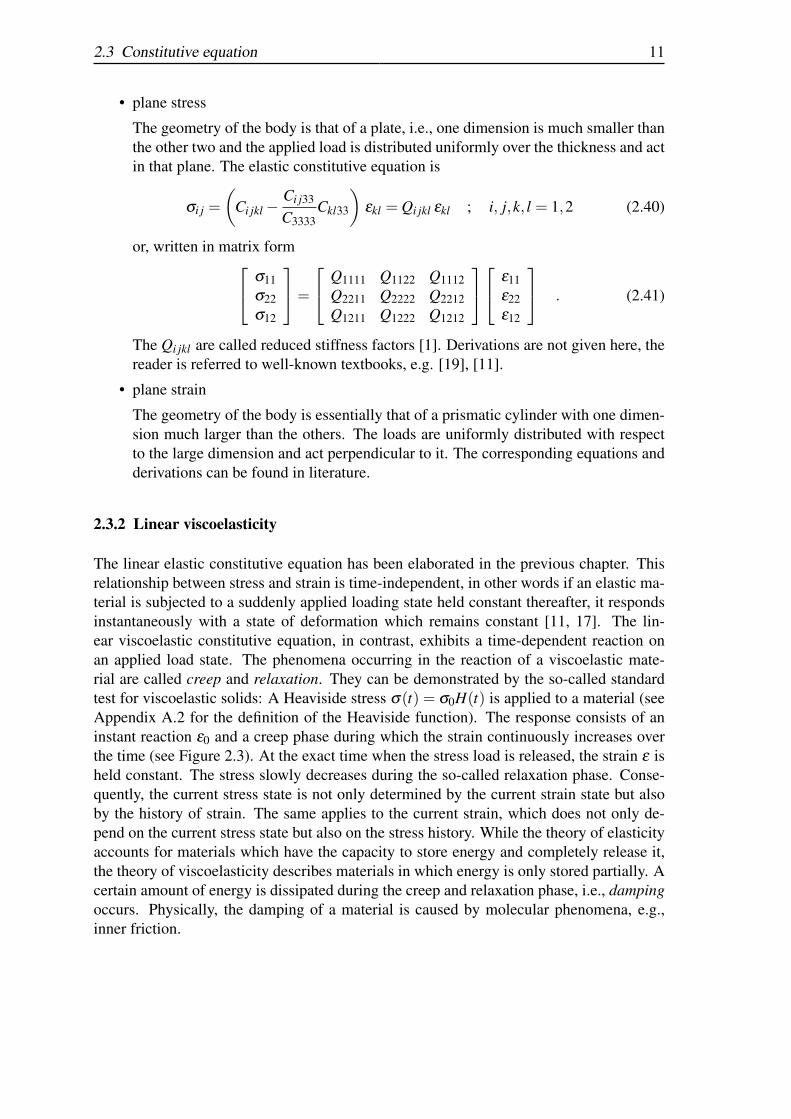
• plane stress
The geometry of the body is that of a plate, i.e., one dimension is much smaller thanthe other two and the applied load is distributed uniformly over the thickness and actin that plane. The elastic constitutive equation is
σi j =(
Ci jkl−Ci j33
C3333Ckl33
)εkl = Qi jkl εkl ; i, j,k, l = 1,2 (2.40)
or, written in matrix form σ11σ22σ12
=
Q1111 Q1122 Q1112Q2211 Q2222 Q2212Q1211 Q1222 Q1212
ε11ε22ε12
. (2.41)
The Qi jkl are called reduced stiffness factors [1]. Derivations are not given here, thereader is referred to well-known textbooks, e.g. [19], [11].
• plane strain
The geometry of the body is essentially that of a prismatic cylinder with one dimen-sion much larger than the others. The loads are uniformly distributed with respectto the large dimension and act perpendicular to it. The corresponding equations andderivations can be found in literature.
2.3.2 Linear viscoelasticity
The linear elastic constitutive equation has been elaborated in the previous chapter. Thisrelationship between stress and strain is time-independent, in other words if an elastic ma-terial is subjected to a suddenly applied loading state held constant thereafter, it respondsinstantaneously with a state of deformation which remains constant [11, 17]. The lin-ear viscoelastic constitutive equation, in contrast, exhibits a time-dependent reaction onan applied load state. The phenomena occurring in the reaction of a viscoelastic mate-rial are called creep and relaxation. They can be demonstrated by the so-called standardtest for viscoelastic solids: A Heaviside stress σ(t) = σ0H(t) is applied to a material (seeAppendix A.2 for the definition of the Heaviside function). The response consists of aninstant reaction ε0 and a creep phase during which the strain continuously increases overthe time (see Figure 2.3). At the exact time when the stress load is released, the strain ε isheld constant. The stress slowly decreases during the so-called relaxation phase. Conse-quently, the current stress state is not only determined by the current strain state but alsoby the history of strain. The same applies to the current strain, which does not only de-pend on the current stress state but also on the stress history. While the theory of elasticityaccounts for materials which have the capacity to store energy and completely release it,the theory of viscoelasticity describes materials in which energy is only stored partially. Acertain amount of energy is dissipated during the creep and relaxation phase, i.e., dampingoccurs. Physically, the damping of a material is caused by molecular phenomena, e.g.,inner friction.

12 2 Continuum mechanics
σ
σ0
ε
ε0
t
t
creep phase
relaxation phase
Figure 2.3: Creep and relaxation
Integral formulation
As has been mentioned above, the stress strain relation of a viscoelastic material requiresthe complete stress-strain history. This memory function of a material can mathemati-cally be described by an hereditary integral. In the one-dimensional case, the viscoelasticconstitutive equation reads
ε(t) =t∫
0
J(t− t)dσ(t)
dtdt . (2.42)
The function J(t) is the so-called creep function. It describes the strain of a of a bodywhich is loaded with a Heaviside stress function as given in Figure 2.4.
σ
σ0
t t
J(t)
J(t) = ε(t)σ0
Figure 2.4: Creep function
The hereditary integral in equation (2.42) can be derived by approximating a non-constantstress function σ(t) with a sequence of infinitesimal step functions (see Figure 2.5). Theapproximated stress is
σ(t)≈∑j
∆σ jH(t− t) . (2.43)
Using the rule of linear superposition, the strain yields
ε(t)≈∑j
∆σ jJ(t− t) , (2.44)

2.3 Constitutive equation 13
σ
dσ(t)
t
σ(t)
t t
Figure 2.5: Derivation of the hereditary integral
where all stress steps, starting at t = 0, are taken into account. Considering infinitesimalsmall stress steps,
ε(t) =t∫
0
J(t− t)dσ , (2.45)
is obtained, which can be written as (dσ(t) = dσ(t)dt dt)
ε(t) =t∫
0
J(t− t)dσ(t)
dtdt . (2.46)
In the three-dimensional case, J is, analogously to the theory of elasticity, replaced by afourth-oder tensor Ji jkl . The viscoelastic constitutive equation is then
εi j(t) =t∫
0
Ji jkl(t− t)dσkl(t)
dtdt . (2.47)
Rheological models
Another, very descriptive derivation for the theory of viscoelasticity is the usage of rheo-logical models. These models consist of the simple elements spring and dash-pot.
The spring is the representation of Hooke’s law in the one-dimensional case, stating thatthe stress is proportional to the strain, i.e.,
σ = Eε . (2.48)
The dash-pot is the representation of the viscous material behavior which states that thestress is not proportional to the strain ε , but to the time rate of change ε
σ = ηdε
dt= ηε . (2.49)

14 2 Continuum mechanics
Viscous behavior is often found in liquids, therefore, translating equation (2.49) into shearstress and shear strain,
τ = µ γ (2.50)
describes the constitutive equation of a viscous fluid with the viscosity coefficient µ .
Linear viscoelastic material behavior is a combination of the two simple cases. Springs anddash-pots can be combined in a parallel manner, which results in a KELVIN-VOIGT model(see Figure 2.6). The corresponding differential equation can be derived by considering
E
η
Figure 2.6: KELVIN-VOIGT model
the equilibrium of forces
1η
σ +1E
ddt
σ =ddt
ε . (2.51)
If springs and dash-pots are arranged sequentially, the MAXWELL model is obtained (seeFigure 2.7). The corresponding differential equation can be derived by considering the
E η
Figure 2.7: MAXWELL model
compatibility of deformation
σ = E ε +ηddt
ε . (2.52)
Both models exhibit weaknesses: A stepwise change of strain results in an infinite stressin the KELVIN-VOIGT model and in the MAXWELL MODEL, the stress always relaxes toa value of 0. The most simple model without these deficiencies is the so-called Three-Parameter-Model. It consists of two springs and one dash-pot, see Figure 2.8. The consti-tutive equation for this model is
pddt
σ = E(
ε +qddt
ε
), (2.53)

2.3 Constitutive equation 15
E1
E2
η
Figure 2.8: Three-Parameter-Model for a solid
withp =
η
E1 +E2E =
E1E2
E1 +E2q =
η
E2. (2.54)
In general, a further combination of KELVIN-VOIGT and MAXWELL models is possible.An arbitrary number of elements can be chosen. The differential equation of such a modelhas the form
N
∑k=0
pkdk
dtk σ =M
∑k=0
qkdk
dtk ε . (2.55)
The parameters pk and qk can be expressed in terms of spring and dash-pot coefficients,however, the expressions become very complicated if many parameters are involved. Atransformation of equation (2.55) into an integral form like equation (2.42) is possible.
Frequency domain formulation
If mechanical systems are loaded harmonically with respect to time, their behavior can beanalyzed in frequency domain. The viscoelastic constitutive equation (2.55) then reads
F σN
∑k=0
pk(iω)k = F εN
∑k=0
qk(iω)k , (2.56)
where F denotes the Fourier-transformation and ω is the excitation frequency. Thus, thedifferential equation is replaced by two polynomials and the time-dependence of equation(2.55) is replaced by a frequency-dependence. Equation (2.56) can be solved for σ(ω)
σ(ω) =
N∑
k=0pk(iω)k
N∑
k=0qk(iω)k
ε(ω) = G(iω) ε(ω) =[Gstorage(ω)+ iGloss(ω)
]ε(ω) , (2.57)
where G(iω) is the complex modulus which can be split up into a real and imaginarypart. The real part Gstorage is called storage modulus because it accounts for the amount ofenergy that is stored while the imaginary part Gloss is called loss modulus since it accountsfor the amount of energy that is lost due to energy dissipation.

16 2 Continuum mechanics
Fractional derivatives
In order to adjust the parameters of the proposed viscoelastic constitutive equation to mea-sured data, it can be useful to introduce fractional derivatives [38]. The physical meaningof fractional derivatives within the framework of rheological models can be explained byconsidering the equation for the spring and the dash-pot. The spring equation
σ = Eε = Ed(0)
dt(0) ε (2.58)
can be interpreted as having a ’0-th derivative’ of the strain, while the dash-pot equation
σ = F ε = ηd(1)
dt(1) ε . (2.59)
has the first derivative of ε with respect to time. A more general element can be definedwith
σ = ηdα
dtαε , α ∈ R+ (2.60)
which introduces the order of derivative as an additional parameter. Such an element isalso called ’spring-pot’ [31]. This model is only suitable to give an idea of the fractionalderivative parameter and in a strict sense, one can not speak of a rheological model anymore because the involved parameters can not be attributed to springs or dash-pots. Despitethis fact, a viscoelastic constitutive equation with fractional derivatives has the advantagethat it can adapt a measured material behavior more easily [46].
The generalized viscoelastic constitutive equation is then
N
∑k=0
pkdαk
dtαkσ =
M
∑k=0
qkdβk
dtβkε . (2.61)
2.4 Auxetic Materials
2.4.1 The term auxetic
The linear elastic constitutive equation of materials was discussed in chapter 2.3.1. Inthe isotropic case, the behavior of a material can be characterized via two independentparameters, e.g., Young’s modulus E and Poisson’s ratio ν . From a continuum mechanicspoint of view, there is no restriction for Poisson’s ratio to be positive, see equation (2.39).
The physical meaning of a negative Poisson’s ratio is shown in Figure 2.9, where a tensileload is applied to an initially undeformed material (dashed line). If the Poisson’s ratiois positive, it exhibits a lateral contraction (see Figure 2.9 a) ) while a material with anegative Poisson’s ratio expands in lateral direction (see Figure 2.9 b) ). Materials withsuch a counterintuitive behavior are referred to as auxetic materials. The term auxetic

2.4 Auxetic Materials 17
a) Non-auxetic b) Auxetic
Figure 2.9: Schematic deformation of a material
comes from the greek word ’αυχετoς ’ meaning ’that which may be increased in size’.There are other terms, for example dilational which actually means widening. In thiscontext, the term arise because solids with a negative Poisson’s ratio easily undergo volumechanges. Another term is anti-rubber which is very descriptive because most rubbers havea Poisson’s ratio close to the isotropic upper limit of 0.5. Thus, auxetic materials representthe exact opposite of rubbery materials. An overview of auxetic materials is given in[14, 15]
2.4.2 Origin of auxetic behavior
From a literature review, it can be stated that the auxetic effect is attributed to a nonstandardmicrostructure [34, 39]. Mostly, simplified models of beam-type microstructures are used.Several models have been discussed for the explanation of the auxetic effect. The mostplausible microstructure which allows for the explanation of the auxetic behavior is a non-convex microstructure. Non-convex, in this context, means that the microstructure featuresre-entrant corners, see Figure 2.10. If a material is composed of these star-shaped cells and
Figure 2.10: Causing mechanism of auxetic material
pulled in longitudinal direction, the kinematic mechanism causes it to expand laterally.Many other types of microstructures have been proposed (see Figure 2.11). The reader isreferred to the publications [14, 47, 51] where a variety of these mechanisms are presented.However, all of them have some kind of re-entrant corners and the causing mechanism isalways similar.

18 2 Continuum mechanics
Figure 2.11: Auxetic microstructures
2.4.3 Naturally occurring materials
Our everyday experience tells us that when a material is stretched, it will become thinnerin cross-section. Nobody expects a material to increase in cross-section which is not sur-prising because there are no known examples for natural materials that behave auxeticallyon the macroscale. On the molecular scale, however, a number of examples exist. The α-cristobalite polymorph of crystalline silica for example is auxetic. A description, includingthe deformation mechanism is given in [14]. Other examples for Auxetics on the molecularscale exist, for example the single-crystal materials arsenic and cadmium [14]. Until now,however, it was not yet possible to create a material consisting only of auxetic moleculesand thus exposing auxetic behavior on the macroscale. Another group of natural auxeticmaterial are biomaterials, although it is difficult to determine exact properties of them inthe natural state. Skin, for example, is said to be auxetic [35, 55], as well as cancerousbone with a cellular microstructure [57]. There might be other examples, however, since itis not possible to perform measurements of material constants, auxetic biomaterials remaina rather speculative phenomenon. Moreover, other effects might influence the behavior ofthese ’materials’, such as muscle contraction or chemical reactions.
2.4.4 Man-made auxetic materials and structures
A variety of man-made auxetic materials have been developed and fabricated in recentyears. One can distinguish between honeycomb-like structures, open-cell foams and poly-meric materials.
Honeycomb-like structures
A representative example for a honeycomb-like structure is the re-entrant honeycombmembrane fabricated by K. EVANS from the University of Exeter. Figure 2.12 shows thematerial and a schematic model. The polymeric material with cell dimensions of ≈ 1mmwas fabricated by laser ablation. Similar microstructures could be produced without great

2.4 Auxetic Materials 19
≈ 1mm
Figure 2.12: Cellular auxetic material
effort, which leads to the possibility of ’tailoring’ a material, i.e., producing a microstruc-ture which has specific characteristics, for example a given Poisson’s ratio.
Foams
The pioneering work in the field of auxetic foams was done by RODERIC LAKES fromthe University of Wisconsin, he was the first to introduce a negative Poisson’s ratio foammaterial [34]. The foam was produced from a conventional low density open-cell polymerfoam by causing the ribs of each cell to permanently protrude inward, resulting in a re-entrant structure. Both conventional and auxetic foams are shown in Figure 2.13.
≈ 2mm
a)auxetic foam b) non-auxetic foam
Figure 2.13: Auxetic and non-auxetic foam

20 2 Continuum mechanics
An analysis of this polymeric cellular material was then given in [7], where the behaviourunder torsional vibration was analyzed and compared to a conventional material. Disper-sion of standing waves and cut-off frequencies were observed. Furthermore, this wavedispersion was studied in a more detailed paper [8], including a numerical investigationof the material. An industrial application is given in [36]. The auxetic foam was used asa seat cushion material. By investigating the pressure distributions on a seated subject, itwas found that the auxetic material exerts a reduced peak pressure.
Polymers
A further group of auxetic materials are liquid crystal polymers (LCPs). Each LCP chain
Figure 2.14: Polymeric auxetic material (schematic)
consists of a series of rods interconnected terminally or laterally by flexible spacers, asshown in Figure 2.14. Then, as the structure is stretched, the rods attached laterally rotateperpendicular to the main chain, pushing neighbouring chains apart. This increases theinter-chain distance and may give rise to the auxetic effect.
2.4.5 Industrial applications
Potential applications for auxetic materials have been shown in many publications. Sincethey are suspected to have good damping characteristics, they could be used as structuralparts for noise insulation[43, 44, 44]. Another direct application is in seals and gaskets. Aconventional gasket tends to be squeezed out between, for example, the flages of a pipe.If the gasket could be made to be auxetic, however, it would contract in on itself, pro-ducing a tighter seal. Auxetic materials could also be used in applications where shockabsorption is of importance. It is suspected that a variety of auxetic materials have betterindentation resistance than their conventional counterparts. The reason is that if an objectimpacts an auxetic material, material flows into the vicinity of the impact as a result oflateral contraction accompanying the longitudinal compression due to the impacting ob-ject. Hence the material densifies under the impact on both the longitudinal and transversedirections, leading to increased indentation resistance. For non-auxetic materials, on the

2.4 Auxetic Materials 21
other hand, material ’flows’ away in the lateral direction, leading to a reduction in densityand, therefore, a reduction in the indentation resistance.
In [22] for example, a study of the implications of using auxetic materials in the designof smart structures is presented. By using auxetic materials as core and piezoelectric ac-tuators as face layers, the shape control of a sandwich beam is investigated. In [10], afastener based on negative Poisson’s ratio foam is designed. The insertion of the fasteneris facilitated by the lateral contraction which the material exhibits under compression. Theremoval is then blocked by the elastic expansion under tension.
Auxetic materials research is still at a stage where no specific materials or applicationshave reached series-production readiness. However, there are many possible applicationswhich show that there might be a great potential in such materials.

22 2 Continuum mechanics

3 CALCULATION OF TRUSS STRUCTURES
In the previous chapter, different microstructures were presented which cause materials tohave a negative Poisson’s ratio. Mostly, beam-type models were used because they providea very descriptive explanation of the auxetic effect. The beam is one of the most importantconstructional element in structural mechanics. A constructional element is called beam ifone physical dimension is considerably larger than the other two. A beam carries lateralload by bending, if the load is parallel to the axis, one speaks of a bar rather than a beam.
A structure consisting of straight beams connected at joints is called truss. Several studiesare known for the calculation of trusses. Since in structural mechanics, the Finite ElementMethod (FEM) is mostly applied in practice, many publications exist with different ele-ment types and formulations for truss structures [4, 58]. As an alternative to the FEM, theBoundary Element Method (BEM) has been developed in recent years for the numericalsolution of various engineering mechanic problems. In this chapter, a Boundary Elementformulation is presented which provides an exact solution for the calculation of plane trussstructures in statics and in frequency domain.
3.1 Basic Equations and Fundamental Solutions
3.1.1 Beam
The most common theory to describe the behavior of a beam is Euler-Bernoulli’s theoryof bending. Assuming that Young’s modulus E and the moment of inertia I are constantover the beam length, it can be written via the well-known fourth order partial differentialequation
EI∂ 4
∂x4 w+ρA∂ 2w∂ t2 = q , (3.1)
where ρ is the density of the beam material and A is the area of cross-section. The time- andspace-dependency of the deflection w = w(x, t) and the vertical load q = q(x, t) was skippedfor the sake of brevity in equation (3.1). In static calculations, Euler-Bernoulli’s theory ofbending is sufficiently accurate, especially for slender beams with a large length/widthratio [3]. However, in the description of beams with a relatively small length/width ratioand in dynamic calculations, the shear deformation and rotatory inertia of a beam requires amore precise theory. Therefore, TIMOSHENKO [52] developed a refined theory of bendingin which the deflection w does not only depend on the rotation ϕ but also on the angle of
23

24 3 Calculation of Truss Structures
wx
qm
`
γ
ϕ
Euler-BernoulliTimoshenko
w
Figure 3.1: Simple beam, shear angle
shear γ at the neutral axis (see Figure 3.1). Thus, the first derivative of the deflection is
∂
∂xw(x, t) =−ϕ(x, t)+ γ(x, t) . (3.2)
The theory can be written in the following coupled system of differential equations[κGA ∂ 2
∂x2 −ρA ∂ 2
∂ t2 κGA ∂
∂x
−κGA ∂
∂x EI ∂ 2
∂x2 −κGA−ρI ∂ 2
∂ t2
]︸ ︷︷ ︸
Bt
[wϕ
]=−
[qm
]. (3.3)
In equation (3.3), G is the shear modulus and m is a momentum load on the beam (seeFigure 3.1). The so-called shear coefficient κ gives the ratio of the average shear strainon a section to the shear strain at the centroid (for details, see, e.g., [53]). Its value isdependent on the shape of cross-section, but also, as pointed out by Cowper [12], on thematerial’s Poisson ratio and, moreover, for dynamic problems on the considered frequencyrange. Different approximations exist, e.g., that of ROARK for only static deflections withκ = 0.9 for a circular and κ = 5/6 for rectangular cross sections [42].
The two coupled differential equations of second order (3.3) can as well be written in onefourth order differential equation by eliminating the state ϕ
EI∂ 4w∂x4 +ρA
∂ 2w∂ t2 −ρI(1+
EκG
)∂ 4w
∂ t2∂x2 +ρAρI
κGA∂ 4w∂ t4
= q− IκGA
(E∂q∂x2 −ρ
∂ 2q∂ 2t
) . (3.4)
Neglecting the shear deformation and rotatory inertia (i.e., G→∞ and ρI→ 0) in equations(3.3) or (3.4), the Euler-Bernoulli beam equation (3.1) is obtained. Here, however, equa-tion (3.3) is used because this form is more suitable for the following considerations.

3.1 Basic Equations and Fundamental Solutions 25
For harmonic loadings q = q(x, t)eiωt and m = m(x, t)eiωt with the same excitation fre-quency ω or only one type of excitation, both responses can also assumed to be harmonicwith this frequency and their amplitudes w and ϕ are described by[
κGA ∂ 2
∂x2 −ρAω2 κGA ∂
∂x
−κGA ∂
∂x EI ∂ 2
∂x2 −κGA−ρIω2
]︸ ︷︷ ︸
Bω
[wϕ
]=−
[qm
]. (3.5)
The fundamental solutions for Timoshenko’s beam theory in frequency domain are theresponses of an infinite beam to a unit impulsive force q∗(x) = δ (x− ξ ) and to a unitimpulsive moment m∗(x) = δ (x− ξ ), respectively, at the point ξ . With δ (x− ξ ), theDirac delta distribution is denoted (see Appendix A.2). Using a short operator notation,the fundamental solution matrix G is defined by
BωG =−Iδ (x−ξ ), (3.6)
or, in detail,[κGA ∂ 2
∂x2 −ρAω2 κGA ∂
∂x
−κGA ∂
∂x EI ∂ 2
∂x2 −κGA−ρIω2
][w∗q(x,ξ ) w∗m(x,ξ )ϕ∗q (x,ξ ) ϕ∗m(x,ξ )
]=−
[δ (x−ξ ) 00 δ (x−ξ )
]. (3.7)
Following the ideas of HÖRMANDER [28], the fundamental solutions can be found from ascalar function ψ via the ansatz[
w∗q(x,ξ ) w∗m(x,ξ )ϕ∗q (x,ξ ) ϕ∗m(x,ξ )
]︸ ︷︷ ︸
G
=
[EI ∂ 2
∂x2 −κGA−ρIω2 −κGA ∂
∂x
κGA ∂
∂x κGA ∂ 2
∂x2 −ρAω2
]︸ ︷︷ ︸
Bcoω
ψ (3.8)
with the matrix of cofactors Bcoω of the operator matrix Bω (see Appendix A.3 for the
definition of the cofactor matrix). With
(Bω)−1 =Bco
ω
det(Bω), (3.9)
the more convenient form
BωG = BωBcoω ψ = det(Bω)Bω(Bω)−1︸ ︷︷ ︸
I
ψ =−Iδ (x−ξ ) (3.10)
is achieved. The two roots of det(Bω) = 0 are
λ1,2 =−ω2
2
( 1c2`
+1c2
s
)± 1
c2`
√(1−
c2`
c2s
)2
+4c2`A
ω2I
, (3.11)

26 3 Calculation of Truss Structures
with the longitudinal and shear wave speeds
c` =
√Eρ
(3.12)
cs =
√κGρ
. (3.13)
Thus, the problem is reduced to find a solution of the iterated Helmholtz operator(∂ 2
∂x2 −λ1
)(∂ 2
∂x2 −λ2
)ψ =−δ (x−ξ )
κGA EI. (3.14)
From several publications, e.g., from CHENG et al. [9], one knows its solution
ψ =1
2κGA EI(λ1−λ2)
[e−√
λ1r√
λ1− e−
√λ2r
√λ2
](3.15)
withr =| x−ξ | . (3.16)
Finally, the operator Bω is applied on the scalar function ψ . The fundamental solutionsdue to a unit force impulse and a unit moment impulse at x = ξ are then found to be
w∗q(x,ξ ) =1
2κGA1
λ1−λ2
[e−√
λ1r√
λ1
(λ1−
κGA−ρIω2
EI
)
−e−√
λ2r√
λ2
(λ2−
κGA−ρIω2
EI
)](3.17a)
ϕ∗q (x,ξ ) =
12EI
2H(x−ξ )−1λ1−λ2
[−e−√
λ1r + e−√
λ2r]
(3.17b)
w∗m(x,ξ ) =−ϕ∗q (x,ξ ) (3.17c)
ϕ∗m(x,ξ ) =
12EI
1λ1−λ2
[e−√
λ1r√
λ1
(λ1−
ρAω2
κGA
)− e−
√λ2r
√λ2
(λ2−
ρAω2
κGA
)].
(3.17d)
More detailed derivations of the fundamental solutions are given in [21] or [45].
In the static case, i.e., for ω → 0, the fundamental solutions simplify to:
w∗q(x,ξ ) =1
12EI
[r3−6
EIκGA
r]
(3.18a)
ϕ∗q (x,ξ ) =− r2
4EI[2H(x−ξ )−1] (3.18b)
w∗m(x,ξ ) =r2
4EI[2H(x−ξ )−1] (3.18c)
ϕ∗m(x,ξ ) =− r
2EI, (3.18d)

3.1 Basic Equations and Fundamental Solutions 27
corresponding to the derivation given in [3].
3.1.2 Bar
If only longitudinal loads act on a beam, it is called bar. The governing equation for thelongitudinal deformation u = u(x, t) is of second order
EA∂ 2u∂x2 −ρA
∂ 2u∂ t2 =−n , (3.19)
where n = n(x, t) is the distributed load in axial direction. For time-harmonic loads n =n(x, t)eiωt with the excitation frequency ω , the response can also be assumed to be time-harmonic. This results in the following differential equation
∂ 2u(x)∂x2 +
(ω
c`
)2
u(x) =− n(x)EA
(3.20)
with the longitudinal wave speed c`, see equation (3.12).
The adequate fundamental solution of the bar equation (3.20), i.e., the axial displacementresponse of an infinite bar to a unit harmonic axial point force n∗(x) = δ (x−ξ ) acting atpoint ξ , is well-known to be [21]
u∗(x,ξ ) =−1
2kEAsin(kr) , k =
ω
c`. (3.21)
Its correctness can easily be demonstrated, since its first and second derivative, respec-tively, is
∂ u∗(x,ξ )∂x
=−1
2EAcos(kr)
∂ r∂x
=−1
2EAcos(kr)[2H(x−ξ )−1] (3.22)
∂ 2u∗(x,ξ )∂x2 =
k2EA
sin(kr)− cos(kr)EA
δ (x−ξ ) , (3.23)
such that
`∫0
[∂ 2u∗(x,ξ )
∂x2 + k2u∗(x,ξ )]
u(x)dx
=−`∫
0
cos(k|x−ξ |)EA
δ (x−ξ )u(x)dx =−u(ξ )
EAfor ξ in [0, `] . (3.24)
In the static case equation (3.21) simplifies to
u∗(x,ξ ) =−r
2EA. (3.25)

28 3 Calculation of Truss Structures
3.2 Integral Equation
The most general methodology to derive from differential equations equivalent integralequations is the method of weighted residuals. The weighted residuum of the beam equa-tion (3.5) is
`∫0
(Bω
[w(x)ϕ(x)
]+[
q(x)m(x)
])T [ w∗q(x,ξ ) w∗m(x,ξ )ϕ∗q (x,ξ ) ϕ∗m(x,ξ )
]dx =
[00
]. (3.26)
As weighting function, the matrix of fundamental solutions is chosen. Performing twointegrations by part and taking into account the filtering effect of the Dirac distribution,the differential operator Bω is shifted from w(x) and ϕ(x) on the matrix of fundamentalsolutions. The following (exact) equation is obtained
[w(ξ )ϕ(ξ )
]=
`∫0
[w∗q(x,ξ ) ϕ∗q (x,ξ )w∗m(x,ξ ) ϕ∗m(x,ξ )
][q(x)m(x)
]dx
+[[
w∗q(x,ξ ) ϕ∗q (x,ξ )w∗m(x,ξ ) ϕ∗m(x,ξ )
][Q(x)M(x)
]−[
Q∗q(x,ξ ) M∗q(x,ξ )Q∗m(x,ξ ) M∗m(x,ξ )
][w(x)ϕ(x)
]]x=`
x=0. (3.27)
The corresponding shear force and bending moment terms are given in Appendix B.
The above described transformation of a differential equation into an equivalent integralequation can similarly be applied to the bar equation (3.20). The bar equation, weightedwith the fundamental solution (3.21)
`∫0
[d2u(x)
dx2 −h2u(x)+n(x)EA
]u∗(x,ξ )dx = 0 (3.28)
is integrated by parts two times over the problem domain, i.e., here, over the bar length `.This gives
[u′(x)u∗(x,ξ )− u(x)
∂u∗(x,ξ )∂x
]`
0+
`∫0
[∂ 2u∗(x,ξ )
∂x2 −h2u∗(x,ξ )]
u(x)dx
=−`∫
0
n(x)EA
u∗(x,ξ )dx . (3.29)

3.3 Boundary (Element) Equations by Collocation 29
Taking the filtering effect of the Dirac distribution δ (x− ξ ) into account, the followingintegral expression for the axial displacement at an arbitrary point ξ ∈ [0, `] is achieved
u(ξ ) =[
EAu′(x)u∗(x,ξ )− u(x)EA∂u∗(x,ξ )
∂x
]x=`
x=0+
`∫0
n(x)u∗(x,ξ )dx
=[N(x)u∗(x,ξ )− u(x)N∗(x,ξ )
]x=`
x=0 +`∫
0
n(x)u∗(x,ξ )dx . (3.30)
The second boundary state N∗(x,ξ ) is given in Appendix B.
3.3 Boundary (Element) Equations by Collocation
In beam problems, always two of the state variables (w, ϕ,M, Q) at each boundary point,i.e., at x = 0 and x = `, are unknown, while in a bar problem only one of the state variables(u, N) has to be determined. Hence, plane framework problems are, in general, a combina-tion of both, so that three of the six state variables (u, w, ϕ, N,M, Q) are unknown at eachof the two boundary points and, consequently, one needs also three boundary equationsat these two boundary points. The simplest way to evaluate the above systems (3.27) and(3.30) at these two points, is to perform point collocation at ξ = 0 and ξ = `, resultingin
[I−K(0,0) F(0,0) K(`,0) −F(`,0)−K(0, `) F(0, `) I+K(`,`) −F(`,`)
]u(0)t(0)u(`)t(`)
=
`∫0
[F(x,0)F(x, `)
] n(x)q(x)m(x)
dx (3.31)
with
K(x,ξ ) =
N∗(x,ξ ) 0 00 Q∗q(x,ξ ) M∗q(x,ξ )0 Q∗m(x,ξ ) M∗m(x,ξ )
(3.32)
F(x,ξ ) =
u∗(x,ξ ) 0 00 w∗q(x,ξ ) ϕ∗q (x,ξ )0 w∗m(x,ξ ) ϕ∗m(x,ξ )
(3.33)
u(x) =
u(x)w(x)ϕ(x)
(3.34)

30 3 Calculation of Truss Structures
t(x) =
N(x)Q(x)M(x)
. (3.35)
System (3.31) has the form
[E] [d] = [r] (3.36)
with the 6× 12 matrix E, the vector of all 12 boundary values d and the load vector r.In Appendix B, equation (3.31) is given in detailed form. Matrix E can be considered asan "element matrix" analogical to an element matrix used in Finite Element calculations.Contrary to the FEM, E is not symmetric and also forces and bending moments appearas degrees of freedom. With equation (3.31), a single beam calculation can easily beperformed because 6 of the overall 12 boundary values are given as boundary conditions.Thus, the remaining 6 unknown values can be calculated with the 6 available equations.Values for the state variables of inner points can be calculated using (3.27) and (3.30).
3.4 Assembling of System Matrix
Plane truss structures are composed of multiple beams which are connected among eachother. It is straightforward to calculate element equation (3.31) for each single beam andtransform it into a global coordinate system. Then, taking into account transition condi-tions at the coupling points of the beams, a system of linear equations for the truss structurecan be assembled. At a first glance, it seems that the calculation is not possible becausethere are only 6 equations for a total of 12 unknown boundary values per beam. However,taking into account the boundary conditions at the supports and transition conditions at theconnection points, 6 equations per beam suffice to calculate a truss structure.
3.4.1 Global Coordinates
As a first step to the assembling of a system matrix, it is meaningful to transform the el-ement equation (3.31) into a global coordinate system. Figure 3.2 shows the local andglobal systems. The local values for the deformation u1,2
loc, w1,2loc, ϕ
1,2loc and the forces and
bending moments M1,2loc , Q1,2
loc, N1,2loc are transformed into a global coordinate system. The
usual sign convention for local values is found in Figure 3.2: At node 1, forces and defor-mations point into opposite directions, while at node 2, they have the same direction. Inthe global coordinate system, both forces and also deformations at node 1 and 2 have the

3.4 Assembling of System Matrix 31
u1loc
ϕ1loc
w1loc
M1loc
Q1loc
N1loc
u2loc
w2loc
ϕ2loc
M2loc
Q2loc
N2loc
u1,M1
w1,F1y
ϕ1,F1x
u2,M2
w2,F2y
ϕ2,F2x
1
2
1
2
α α
local: global:
Figure 3.2: Local and global coordinates
same direction. Using the sine and cosine functions, it can be seen thatu1
locw1
locϕ1
locM1
locQ1
locN1
loc
=
cos(α) −sin(α)sin(α) cos(α) 0
1−1
0 −cos(α) −sin(α)sin(α) −cos(α)
︸ ︷︷ ︸
T1
u1
w1
ϕ1
M1
Q1
N1
(3.37)
andu2
locw2
locϕ2
locM2
locQ2
locN2
loc
=
cos(α) −sin(α)sin(α) cos(α) 0
1−1
0 cos(α) sin(α)−sin(α) cos(α)
︸ ︷︷ ︸
T2
u2
w2
ϕ2
M2
Q2
N2
. (3.38)
Incorporating equations (3.37) and (3.38) into (3.36), an element equation in global coor-dinates is obtained
[E][
T1 00 T2
]︸ ︷︷ ︸
E
[d]= [r] . (3.39)
The vector d contains all 12 boundary values in global coordinates. The load vector r canbe transformed analogically.

32 3 Calculation of Truss Structures
3.4.2 Assembling
The assembling of the system matrix is done in the following way:
• rows:The element equations of the single beams are arranged row-wise, i.e., the first sixrows of the system matrix contain entries of equations for element 1, rows 7 through12 are occupied by entries of element equation 2 and so on.
• columns:The columns of the system matrix represent the unknown boundary values of thebeam ends (nodes). It depends on the boundary and transition conditions whichunknowns are represented, however, the first columns represent unknowns of node1, then 2 and so on.
Which unknowns are used in the columns and how exactly they are arranged (”accordingto the boundary/transition conditions”) is demonstrated by the following examples.
3.4.3 Boundary Conditions
As a first example, a single beam problem with rigid supports on both ends is considered,see Figure 3.3. The deformation values are all set to 0, except for the deflection w on
w
u
x
1 2
w
Figure 3.3: Single beam example
the right hand side. No further loads act on the system, so the load vector on the righthand side is 0. Figure 3.4 shows how the boundary conditions are incorporated into theelement matrix. On the left hand side, the element matrix E (see equation (3.39) ) is shownwith different hatchings for the columns of deformations and forces of nodes 1 and 2. Onthe right hand side, the Figure shows the system matrix (denoted by A) and load vector(denoted by f).
The columns of the deformation values of the matrix E are deleted, except for the columnof w2 which is multiplied with w and put into the load vector on the right hand side. Thecolumns for M1,Q1,N1,M2,Q2,N2 remain as unknowns in the system matrix A whichnow has 6 rows and 6 columns. The non-symmetric system can be solved with a standardsolver for linear equations, e.g. LU-decomposition. With equations (3.27) and (3.30),deformation values at arbitrary points along on the beam can be calculated.

3.4 Assembling of System Matrix 33
u1 w1 ϕ1 M1 Q1 N1 u2 w2 ϕ2 M2 Q2 N2
·0·w
M1 Q1 N1 M2 Q2 N2
=
E A
f
Figure 3.4: Assembling of system matrix
3.4.4 Transition Conditions
The application of transition conditions at the connection points of truss structures is morecomplicated than in a deformation-based calculation procedure like the FEM. This is due tothe fact that in the boundary element equation (3.31), forces and bending moments appearas degrees of freedom. If a rigid connection of n beams is considered (see Figure 3.5), thedeformation values of all beam ends must be equal, i.e.,
u1 = u2 = · · ·= un (3.40a)w1 = w2 = · · ·= wn (3.40b)ϕ1 = ϕ2 = · · ·= ϕn . (3.40c)
The forces and bending moments, however, must satisfy the condition that their sums are0, so
∑Fx = 0 = Fx1 +Fx2 + . . .Fxn (3.41a)
∑Fy = 0 = Fy1 +Fy2 + . . .Fyn (3.41b)
∑M = 0 = M1 +M2 + . . .Mn . (3.41c)
The example in Figure 3.6 is considered to demonstrate the assembling. For all threebeams, element matrices E and load vectors r are set up in a global coordinate system. Thesix equations of each element are arranged on top of each other in the system matrix. Withun(x) and tn(x), deformation and force vectors of beam n are denoted, see also equations

34 3 Calculation of Truss Structures
1
2
n
1
2
n
Figure 3.5: Transition conditions of a rigid connection
(3.34) and (3.35). Again, according to the given boundary conditions of the beams, entriesof the element matrices are deleted or shifted to the right hand side. In this case, entriesu1(0), u2(`) and t3(`) are deleted, since they are known to be 0. The complementary statevariables t1(0), t2(`) and u3(`) are put into the system matrix. At the connection point,deformation values must be equal, so the entries of u1(`), u2(0) and u3(0) are put intothe same columns of the system matrix A. In order to satisfy the condition that the sumof forces and bending moments at the connection point must be 0, the following is done:matrix block of t1(`) is put into the system matrix with a negative sign. Entries of t2(0)and t3(0) are then written below these two blocks. Thus,
−t1(`) = t2(0)+ t3(0) (3.42)
is satisfied. In the system matrix, only t2(0) and t3(0) appear as degrees of freedom,but t1(`) can easily be calculated via (3.42). Figure 3.7 shows the prescribed procedureschematically. The resulting system of linear equations is quadratic and thus can be com-puted with an adequate solver.
3.4.5 Combined Transition/Boundary Conditions
In an arbitrary truss structure, a combination of boundary and transition conditions mayoccur. Figure 3.8 shows such a case: at the connection point of two beams is a vertical
1
2
3
Figure 3.6: Simple truss structure

3.4 Assembling of System Matrix 35
!!!!!
""""""
######
$$$$$
%%%%%
&&&&&&&&&&&&&&&&&&&&
'''''''''''''''
((((((((((((((((((((((((((((((
))))))))))))))))))))))))))))))
*************************
+++++++++++++++++++++++++
,,,,,,,,,,,,,,,,,,
------------------
..................
//////////////////
000000000000000000000000000000000000
111111111111111111111111111111
222222222222222
333333333333333
444444444444444
555555555555555
6666666666666666666666666666666666666666
7777777777777777777777777777777777777777
8888888888888888888888888
9999999999999999999999999
1
2
3
·(−1) ·(−1)
un(0) tn(0) un(`) tn(`) rn
t1(0) u1(`) t2(0) t3(0) t2(`) u3(`) f
=
Figure 3.7: Assembling of system matrix
support. Firstly, the two beams are treated as if there was no support, i.e., the matrix
12
Figure 3.8: Connection point of two beam with a vertical support
entries for the deformation are put in the same columns. Entries for the forces and bendingmoments are also put in the same columns, entries of beam 1 are multiplied with −1, seeFigure 3.9. After this, the support at the connection point is considered. The deflectionis set to 0 here, thus, the entries for w can be erased. The blank column is used for theunknown force at the connection point. For this, the following is done: a load of size 1is put on the right end of the left beam. The resulting load vector is inserted into the freecolumns of the system matrix. The resulting system can be solved. In principle, the loadcan as well be put on the left end of the right beam.
3.4.6 Solving the System Matrix
In general, the system matrix is fully populated and not symmetric. It is not possible togenerate a symmetric matrix with the prescribed method, however, if the element equa-

36 3 Calculation of Truss Structures
1
2
·(−1) ·(−1)
u1(`) t2(0) u1(`) t2(0)
1
Figure 3.9: Assembling of system matrix
tions (rows in system matrix) and the degrees of freedom (columns in system matrix) arearranged in a specific way, a banded system matrix can be obtained. This is a clear parallelto the Finite Element Method, where one also has local element matrices, which are putinto a symmetric, banded system matrix. The example structure shown in Figure 3.10 isused to explain the implication of a ”good” element numbering. The structure consists of
a) example structure b) discretization
Figure 3.10: Example structure and discretization scheme
10×10 square cells with four beams on the edges. The system matrix for the 220 beamsand 121 nodes is assembled for two different discretizations. In the first discretization,the numbering of the elements is done randomly and in the second one, node numbersand beam numbers start at the left bottom of the structure, going up line-wise as shown inFigure 3.10. The resulting system matrices are shown in Figure 3.11. If the discretizationis done randomly, matrix entries are scattered over the entire matrix. To be precise, thereare groups of entries: the six equations of one element (six lines) and degrees of free-dom of one node (columns) form one group. The second system matrix exhibits a bandedstructure. Since the element numbering is done line-wise, there is a band of entries on thediagonal of the matrix. Below the diagonal, there is another band of entries because the el-ement entries of one line of elements are connected with the neighboring lines of elements.

3.4 Assembling of System Matrix 37
0 600 1200
0
600
1200
a) random discretization0 600 1200
0
600
1200
b) ordered discretization
Figure 3.11: Occupancy of system matrix
In this discretization, the bandwidth of the system matrix is determined by the maximumdifference of node numbers of a beam element. However, it must be emphasized that thisstatement can not be generalized like in the FEM.
3.4.7 Example Calculation
The following plane truss structure (see Figure 3.12) is considered which consists of sixrigidly connected beams. The beams consist of steel (Young’s modulus E = 2.1 · 1011
P
wp
q0(ω)
2m
1m
1m
Figure 3.12: Plane frame of six rigidly fixed beams: Geometry, support, and loading
N/m2, Poisson’s ratio ν = 0.3, and material density ρ = 7850 kg/m3) with a rectangularcross section A with b = h = 0.1m. The shear coefficient is chosen to be κ = 5/6. The

38 3 Calculation of Truss Structures
excitation is a frequency-dependent point load of intensity q0(ω) = 1000 N acting at thecentre of the upper beam.
Euler-Bernoulli / Timoshenko
Firstly, a comparison is made between Euler-Bernoulli’s theory of bending and Timo-shenko’s theory of bending. The truss structure is calculated with the prescribed boundaryelement method for both theories. Euler-Bernoulli results can easily be obtained by set-ting κGA→ ∞. The truss structure is calculated up to a frequency of 900 Hz, increasingthe excitation frequency in steps of 10 rad/sec (≈ 1.592 Hz). For comparison, the deflec-tion response wP at the center point P on the first frame floor is plotted in Figure 3.13
1e-09
1e-08
1e-07
1e-06
1e-05
1e-04
0.001
0.01
0.1
1
0 100 200 300 400 500 600 700 800 900
defle
ctio
n (m
)
frequency (Hz)
91.2108.2
334.4 433.1
TimoshenkoEuler-Bernoulli
Figure 3.13: Comparison between Euler-Bernoulli and Timoshenko theory
for both theories over the considered frequency range. The static deflection (ω → 0) is3.242 ·10−6m for Euler-Bernoulli’s theory and 3.100 ·10−6m for Timoshenko’s theory ofbending, which is a difference of less than 5%. Thus, the shear deformation is negligible,which could be expected because the beams have a length/width ratio of of 10 and 20,respectively. This statement about static calculations can be found in many publications,for example [3]: ”... the difference of beam reactions determined by Euler-Bernoulli’sand by Timoshenko’s beam theory depends on the actual geometry, but is in general verysmall.”.

3.4 Assembling of System Matrix 39
In a frequency range up to 300Hz, there is still no significant difference between boththeories. However, in higher frequencies, starting from the third eigenfrequency, a shiftof eigenfrequencies can be observed. The shift is small at the third eigenfrequency butincreases for the higher frequencies.
BEM / FEM
Since the Finite Element Method is the most established numerical procedure for the cal-culation of engineering structures, a comparison is made between the prescribed BoundaryElement Method and the FEM. Two Finite Element calculations are performed using 32and 64 Timoshenko beam elements. As stiffness matrix, a cubic Lagrange-element with4 degrees of freedom (derived from an 8-degrees of freedom element via static condensa-tion) is used (see Appendix C). The mass matrix takes into account the rotatory inertia, adetailed derivation of the element is given in [30]. In longitudinal direction, linear shapefunctions are used, the resulting element matrix can also be found in [30]. In Figure 3.14,the results of the BEM and FEM calculations are shown. Again, the deflection wP at the
1e-09
1e-08
1e-07
1e-06
1e-05
1e-04
0.001
0.01
0.1
1
0 100 200 300 400 500 600 700 800 900
defle
ctio
n (m
)
frequency (Hz)
91.2108.2
334.4 433.1
BEMFEM 64 elementsFEM 32 elements
Figure 3.14: Comparison between BEM and FEM
center point P on the first frame floor is plotted versus the excitation frequency. As canbe seen, the BEM and FEM results show a good agreement up to a frequency of approx-imately 250 Hz. With a higher excitation frequency, however, the FEM results becomeinaccurate. The coarse FEM descretization with 32 elements is less precise than the finer

40 3 Calculation of Truss Structures
discretization with 64 elements - a typical result of the FEM where the solution usuallyconverges to the exact solution when the mesh is made finer.
More results concerning the comparison between the proposed method and the FEM canbe found in [21, 2].

4 MICROMECHANICS AND HOMOGENIZATION
Nearly all materials present a certain heterogeneous microstructure, although they seemto be homogeneous on a macroscopic scale. Heterogeneities such as cracks, cavities, in-clusions, laminations, grain boundaries or irregular crystal lattices may occur on a micro-scopic scale but still the macroscopic behavior can be homogeneous. A good example forsuch a material is steel, which clearly has a heterogeneous microstructure but exhibits anisotropic behavior on the macroscale. If one were to attempt to perform a direct numericalsimulation of such a heterogeneous material, the consideration of all microscale detailswould require an extremely fine spatial discretization. The resulting system of equationswould contain literally billions of numerical unknowns and would be beyond the capac-ity of computing machines for the foreseeable future. Furthermore, a complete, detaileddescription of a micro-heterogeneous structure is in many cases not possible or necessary.For these reasons, homogenization techniques were developed which aim at predicting theoverall, effective behavior of heterogeneous structures. The literature on the homogeniza-tion problem is very extensive. A good overview can be found in [37, 60, 20].
4.1 Representative Volume Element
The principle of homogenization can be explained as follows. A body Ω with a char-acteristic length scale L is considered (see Figure 4.1). The surface of Ω is termed Γ
which is subdivided into Γt and Γu with Γ = Γu ∪Γt . On Γu, the displacements are pre-scribed and on Γt , the tractions are prescribed. The body consists of a material with amicrostructure which has a characteristic length scale `. Microstructure ingredients suchas matrix-inclusions, granular micro-topologies, etc. have the characteristic length scale d(see Figure 4.1).
For the analysis on the macroscopic length scale L, the body Ω is replaced by a similar butquasi-homogeneous body Ω∗. The body Ω∗ is bounded by the same external boundaries Γtand Γu with the same prescribed tractions and displacements but contrary to Ω, it consistsof a homogeneous material with yet unknown properties. The aim of the homogenizationprocess is to calculate the properties of Ω∗ such that its mechanical behavior is equiva-lent to that of Ω. Thus, the microstructure is replaced by a homogeneous medium whichrepresents the smeared microstructural behavior.
In order to find properties of the homogeneous material, a specific portion of the mi-crostructure is considered. From this portion, the properties of the corresponding homoge-neous material are calculated. Since the homogeneous material must have approximately
41

42 4 Micromechanics and Homogenization
P
L
Ω
P
L
Ω∗
`
d
RVE
Γt Γu Γ∗t Γ∗u
Figure 4.1: Principle of homogenization
the same mechanical properties as the microheterogeneous body Ω, this portion must in-clude all important details of the microstructure. Therefore, it is called RepresentativeVolume Element (RVE). For the volume element to be representative, all microstructuraldetails must be included in a statistically correct manner, otherwise the RVE does not re-flect the microstructure correctly and the homogeneous properties to be calculated willalso not be correct. Thus, the size of the RVE must be large enough to contain all neces-sary information for the description of the given microstructure so the characteristic lengthscale d has to be much smaller than `. On the other hand, the size of the RVE can not betoo big because it is assumed to be a material point on the macroscopic scale L. Thus, forthe choice of an appropriate RVE the condition
d ` L (4.1)
must be fulfilled. This condition is termed scale separation. Many authors also speak ofa structural hierarchy [32] of materials. The scale difference that is required depends onmany factors, so no numerical value can be given.
Besides the scale separation, the condition of macroscopic homogeneity must be fulfilled.This means that the microscopic details must be distributed homogeneously within thebody Ω. If this is not the case, no appropriate RVE can be found and it does not makesense to calculate effective properties. An example for a macroscopically inhomogeneousmaterial is a graded material, i.e., a material which has a continuous variation of materialproperties.
Within the scale consideration shown in Figure 4.1, a material point on the macroscaleis assigned a volume portion on the microscale. To define a homogeneous mechanicalequivalent to the heterogeneous RVE, the volume average of the volume V of the stress

4.2 Classical homogenization approaches 43
and strain, respectively is taken
〈σi j〉=1V
∫V
σi j(x)dV (4.2)
〈εi j〉=1V
∫V
εi j(x)dV , (4.3)
where the symbol 〈·〉 denotes that 〈σi j〉 and 〈εi j〉 are averaged quantities.
If the homogeneous material is assumed to be purely elastic, the constitutive equation onthe macroscale is
〈σi j〉= C∗i jkl 〈εkl〉 , (4.4)
with the effective elasticity tensor C∗i jkl which is is defined as the relation between the twoaveraged quantities 〈σi j〉 and 〈εkl〉.
4.2 Classical homogenization approaches
4.2.1 Voigt - Reuss bounds
A classical technique to determine effective properties of microstructured materials is thecomputation of upper and lower bounds according to VOIGT [56] and REUSS [41]. Thetheory is based on HILL’s condition which states that the strain energy on the microscalemust be equal to the strain energy on the macroscale. Thus,
〈W micro〉 != W macro (4.5)12〈σσσ(x) : εεε(x)〉 !=
12〈σσσ(x)〉 : 〈εεε(x)〉 (4.6)
must be satisfied (see equation (2.12) for the definition of the strain energy).
Within the computation of VOIGT bounds for the material properties, the RVE is subjectedto a number of reference deformation states. It is assumed that the microscopic strain stateis equal in every spatial point of the RVE, i.e.,
〈εi j〉= εi j(x) = const . (4.7)
The implication of this assumption can be pictured by considering a one-dimensional two-phase material. The state of strain is assumed to be uniform over the whole RVE, which canonly be accomplished by re-ordering the two phases of the material in parallel manner (seeFigure 4.2). As boundary conditions, the displacements along boundaries are prescribed.The VOIGT bound provides upper bounds for the sought material parameters.

44 4 Micromechanics and Homogenization
specifieddisplacement
specifieddisplacement
constant strain
Figure 4.2: Intuitive interpretation of VOIGT approximation
An analogous approach was introduced by REUSS. Contrary to VOIGT, the state of stressis assumed to be constant, i.e.,
〈σi j〉= σi j(x) = const . (4.8)
The interpretation of this approach is shown in Figure 4.3. Since the stress is assumed to
specifiedtraction
specifiedtraction
constant stress
Figure 4.3: Intuitive interpretation of REUSS approximation
be constant over the RVE, the two phases are put in series and the traction is prescribedalong the boundaries. The REUSS bound provides lower bounds for the sought materialparameters.
For the special case of materials with n phases which have piecewise constant properties,the VOIGT and REUSS bounds can be calculated as [37]
C∗(Voigt) =n
∑α=1
cαCα (4.9)
C∗−1(Reuss) =
n
∑α=1
cαC−1α , (4.10)
where Ci are the properties of the phases and ci are the volume fractions of the phases.The real properties of the material lie in-between these bounds
C∗(Reuss) < C∗ < C∗(Voigt) . (4.11)
The quality of these bounds heavily depends on the considered microstructure. For fiberreinforced materials, for example, the VOIGT bound may even deliver an exact solution.This is the case if the fibers are aligned in one direction and are perfectly bonded. TheVOIGT bound then delivers the exact solution for the Young’s modulus in direction of the
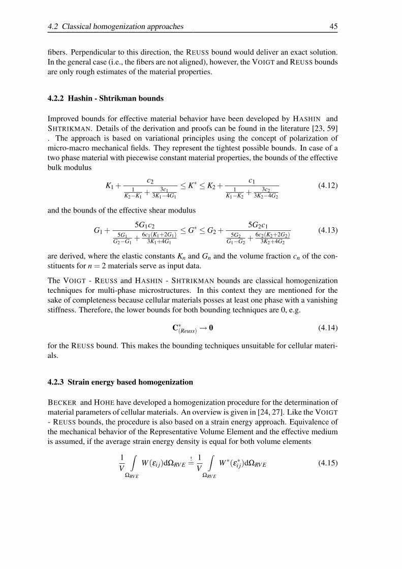
4.2 Classical homogenization approaches 45
fibers. Perpendicular to this direction, the REUSS bound would deliver an exact solution.In the general case (i.e., the fibers are not aligned), however, the VOIGT and REUSS boundsare only rough estimates of the material properties.
4.2.2 Hashin - Shtrikman bounds
Improved bounds for effective material behavior have been developed by HASHIN andSHTRIKMAN. Details of the derivation and proofs can be found in the literature [23, 59]. The approach is based on variational principles using the concept of polarization ofmicro-macro mechanical fields. They represent the tightest possible bounds. In case of atwo phase material with piecewise constant material properties, the bounds of the effectivebulk modulus
K1 +c2
1K2−K1
+ 3c13K1−4G1
≤ K∗ ≤ K2 +c1
1K1−K2
+ 3c23K2−4G2
(4.12)
and the bounds of the effective shear modulus
G1 +5G1c2
5G1G2−G1
+ 6c1(K1+2G1)3K1+4G1
≤ G∗ ≤ G2 +5G2c1
5G2G1−G2
+ 6c2(K2+2G2)3K2+4G2
(4.13)
are derived, where the elastic constants Kn and Gn and the volume fraction cn of the con-stituents for n = 2 materials serve as input data.
The VOIGT - REUSS and HASHIN - SHTRIKMAN bounds are classical homogenizationtechniques for multi-phase microstructures. In this context they are mentioned for thesake of completeness because cellular materials posses at least one phase with a vanishingstiffness. Therefore, the lower bounds for both bounding techniques are 0, e.g.
C∗(Reuss)→ 0 (4.14)
for the REUSS bound. This makes the bounding techniques unsuitable for cellular materi-als.
4.2.3 Strain energy based homogenization
BECKER and HOHE have developed a homogenization procedure for the determination ofmaterial parameters of cellular materials. An overview is given in [24, 27]. Like the VOIGT
- REUSS bounds, the procedure is also based on a strain energy approach. Equivalence ofthe mechanical behavior of the Representative Volume Element and the effective mediumis assumed, if the average strain energy density is equal for both volume elements
1V
∫ΩRV E
W (εi j)dΩRV E!=
1V
∫ΩRV E
W ∗(ε∗i j)dΩRV E (4.15)

46 4 Micromechanics and Homogenization
where W and W ∗ denote the strain energy of the heterogeneous and homogeneous mediumfor equivalent strain states. Equivalence of the micro and macro strain states εi j, ε∗i j isassumed if the volume average of the infinitesimal strain tensors is equal
1V
∫ΩRV E
εi jdΩRV E =1V
∫ΩRV E
ε∗i jdΩRV E . (4.16)
If a linear elastic behavior of the material on the macroscale is assumed, the followingvalues for the tensorial components are derived
Ci jkl =
2W ∗(ε(i j))1
ε∗2(i j)
if i = j,k = l, i = k12W ∗(ε(i j))
1ε∗2
(i j)if i 6= j,k 6= l, i = k, j = l(
W ∗(ε(i j),ε(kl))−W ∗(ε(i j))−W ∗(ε(kl))
) 1ε∗(i j)ε
∗(kl)
if i = j,k = l, i 6= k14
(W ∗(ε(i j),ε(kl))−W ∗(ε(i j))−W ∗(ε(kl))
) 1ε∗(i j)ε
∗(kl)
if i 6= j,k 6= l, i 6= k or j 6= l12
(W ∗(ε(i j),ε(kl))−W ∗(ε(i j))−W ∗(ε(kl))
) 1ε∗(i j)ε
∗(kl)
if i = j,k 6= l
. (4.17)
W ∗(ε(i j),ε(kl)) denotes the strain energy density in the Representative Volume Elementsubjected to a strain state where all components of the strain tensor except ε(i j) and ε(kl)are equal to 0. The brackets () denote that no summation is performed. Thus, the Repre-sentative Volume Element is considered to be deformed by a number of reference strainstates for which the strain energy has to be evaluated. The procedure was developed forcellular materials, where the cell walls consist of straight beams. Deformations and strainenergy can be calculated analytically in this case. A generalization for more general mi-crostructure geometries is given in [25, 26].
4.2.4 Surface average based approach
Within the scale consideration shown in Figure 4.1, a material point on the macroscaleis assigned a volume portion on the microscale. To define a homogeneous mechanicalequivalent to the heterogeneous RVE, a surface average based approach is used. The stressdistribution in the Representative Volume Element consisting of the given microstructureis assumed to be equivalent to a stress distribution of the effective medium if
1Γ
∫Γi
RV E
ti dΓ =1Γ
∫Γi
RV E
〈ti〉dΓ (4.18)
holds, where ti is the traction vector on the surface Γ of the Representative Volume Elementand Γi is a certain part of its boundary. Equation (4.18) describes a redistribution of the

4.2 Classical homogenization approaches 47
stress components along the surface of the Representative Volume Element during thehomogenization process. A second equivalence condition interrelates the strain states onthe microscopic and macroscopic scale. An average strain state for the RepresentativeVolume Element is defined by means of the difference in the displacements of oppositesurfaces of the volume element. If the difference in the displacements of opposite surfacesis not constant along the surface, the surface integral of this quantity is taken. Thus, themacroscopic strain can be expressed by
〈εi j〉=1
2V
∫ΓRV E
(uin j +u jni
)dΓ, (4.19)
where V denotes the volume of the RVE and ni are the components of the outward normalvector on ΓRV E . Thus, the heterogeneous microstructure is smeared over the RVE (see Fig-ure 4.4). With the averaged stress and strain, the effective macroscopic material properties
σσσ ,εεε 〈σσσ〉,〈εεε〉
Figure 4.4: Stress and strain on the micro- and macroscale
are calculated via〈σi j〉= C∗i jkl 〈εkl〉 , (4.20)
with the effective elasticity tensor C∗i jkl which is defined as the relation between the twoaveraged quantities 〈σi j〉 and 〈εkl〉.
The advantage of this approach is that it only requires the tractions and deformations onthe boundary of the RVE. No energetic considerations like in the strain energy based ho-mogenization are made. Thus, it can not only be applied in the static case, but also indynamics. Since the materials discussed in this work are assumed to have a periodic mi-crostructure, it is meaningful to do a dynamic calculation in frequency domain. The reasonis that in frequency domain, periodic boundary conditions can be applied to the RVE. Intime domain, this is not possible because wave propagation phenomena take place. Thus,if a wave is running through the RVE, the tractions and displacements on one edge aredifferent from the tractions and displacements on the opposing edge. It is not possible tofulfill the periodicity, which is postulated from the fact that the material consists of equallyshaped cells. In a frequency domain calculation, in contrast, the RVE is situated in a steadystate where periodicty can be fulfilled.

48 4 Micromechanics and Homogenization
Calculation on Microscale
The aim of homogenization is to calculate effective properties, which in the elastic casemeans that the components of C∗i jkl of equation (4.4) need to be found. C∗i jkl has 21 inde-pendent components in the general, anisotropic case. The RVE is subjected to a number ofstrain states. A useful choice of load states is
〈σi j〉 or 〈εkl〉=
β 0 00 0 00 0 0
,
0 0 00 β 00 0 0
,
0 0 00 0 00 0 β
,
0 β 0β 0 00 0 0
,
0 0 00 0 β
0 β 0
,
0 0 β
0 0 0β 0 0
. (4.21)
The RVE can either be subjected to a strain load where the stress is computed or vice versa.The load factor β can be chosen arbitrarily. The states in (4.21) assure that all unknownsin C∗i jkl can be computed. If the cases are not independent, linear combinations of theequations occur and there are not enough equations to compute all tensor components ofC∗i jkl [13].
In 2-D, 3 independent load cases suffice. To assure that all material parameters can bedetermined, the three loadcases shown in Figure 4.5 can be applied. If the plane stress
ε11 6= 0 ε22 6= 0 ε12 6= 0
Figure 4.5: Independent load cases in 2-D
case is considered, all Qi jkl of equation (2.41) can be calculated. This can easily be seen,because the three loadcases correspond to the three rows of equation (2.41).
Boundary Conditions
The cellular structures are assumed to be periodic, i.e., they consist of equally shaped unitcells. If the microstructure is deformed, neighboring cells undergo the same deformationpattern. The whole macroscopic body consists of identical parts that fit into each other. InFigure 4.6, a two-dimensional unit cell is shown in deformed and undeformed state. The

4.2 Classical homogenization approaches 49
I
II
III
IV
1
2 3
4
Figure 4.6: Periodic boundary conditions
corner nodes are named with arabic numbers 1 to 4 and the edges are named with romannumbers I to IV . Periodic boundary conditions are achieved by pairing opposite facesand linking the corresponding degrees of freedom with each pair of faces. Thus, for thedisplacement vectors u of the nodes or edges, the following symbolic equations must befulfilled
uII = uIV +u2 ; uIII = uI +u4 ; u3 = u2 +u4 . (4.22)
The displacements at the ’slave faces’, II and III, are determined by those of the ”masterfaces”, I and IV , and of the ’master nodes’ 2 and 4. See also [24, 5] for a more detaileddescription. If the stresses t are discretized in addition to the displacements like in themethod described in chapter 3, they have to fulfill anti-periodic conditions, i.e.,
tII =−tIV ; tIII =−tI ; . (4.23)
For unit cells which are symmetric in an undeformed and deformed state, the periodicboundary conditions simplify to symmetric boundary conditions (see Figure 4.7). Due
Figure 4.7: Periodic boundary conditions due to symmetry
to the symmetry of unit cell and boundary conditions, the deformations on the left edge

50 4 Micromechanics and Homogenization
correspond to the deformations on the right edge and the tractions on the upper edge areequal to the tractions on the lower edge.
The periodicity of the boundary conditions needs to be fulfilled in a static calculation aswell as in a dynamic calculation. This makes a dynamic calculation in frequency domainmeaningful.
4.2.5 Unit Cell versus RVE
Within this work, cellular solids are considered which consist of simple beams. Suchstructures are found quite often in literature, they can represent sandwich cores or sim-plified models of foam-like materials. As has been mentioned before, it is assumed thatthe material is periodic, i.e., it consists of equally shaped cells. For sandwich cores, thisassumption is well justified, real materials, of course, have an imperfect microstructure,where neighbouring cells have a slightly different geometry. The cork tree, for example,consists of hexagonal cells as can be seen in Figure 4.8. A model for this material is
Figure 4.8: Microstructure of cork, idealized model and unit cell
also shown in Figure 4.8. The model consists of perfect hexagonal cells, neglecting smallimperfections of the real material. In order to calculate effective, homogeneous materialproperties, this model would be sufficiently accurate to represent the microstructure. If theassumption of periodicity is made, it is very easy to find a RVE, because if the microstruc-ture consists of identical units, the smallest unit contains all information and is thereforerepresentative. In statics, effective properties can be calculated from this single unit cell.In a frequency domain calculation, however, one unit cell does not suffice to obtain repre-sentative results. The reason is that higher modes of deformation may occur when usinga different number of unit cells. This can be explained by considering the example givenin Figure 4.9. A unit cell is loaded with a force on the left and right hand side. The cell iscalculated in frequency domain, i.e., the load is harmonic and thus, the resulting strain
ε =∆`
`(4.24)
is also harmonic. Another calculation is done using 3× 3 cells. Both strains are plottedover a frequency range of 0..106 Hz in logarithmic scale, see Figure 4.10. On the left handside, the whole frequency range is plotted, whereas on the right hand side, only a small

4.2 Classical homogenization approaches 51
`
`
Figure 4.9: Example calculation of 1 and 3×3 unit cells
range is plotted. It can be seen that the results from both calculations are not identical. Atapproximately 3.4 ·105 Hz, an eigenfrequency is missing in the single unit cell calculationand at 2.3 · 105 Hz, the eigenfrequencies of both calculations are different. Therefore,it is necessary to calculate multiple unit cells to obtain characteristic microscale results.A simple and pragmatic approach is to calculate a specific number of unit cell and thenaverage the results.
1e-09
1e-07
1e-05
0.001
0 500000 1e+06
stra
in
frequency
1 unit cell3x3 unit cells
1e-08
1e-07
1e-06
1e-05
200000 250000 300000 350000
stra
in
frequency
1 unit cell3x3 unit cells
Figure 4.10: Strain of 1 and 3×3 unit cells

52 4 Micromechanics and Homogenization

5 OPTIMIZATION
The term optimization refers to the study of problems in which one seeks to minimize ormaximize a function by systematically choosing the values of variables from an allowedset. In the context of this work, optimization techniques are used to obtain macroscopicmaterial parameters, i.e, ’try to find material parameters on the macroscopic scale whichdescribe the micromechanical properties as good as possible’.
Within the scope of this work, the Simplex Method and the Sequential Quadratic Program-ming Method are used. They represent gradient-based optimization techniques. These al-gorithms often exhibit weaknesses in non-convex problems, which means that they can runinto local minima of the search space. Therefore, two global optimization techniques, aGenetic Algorithm and a Neural Network are also applied to the optimization problem.
5.1 Simplex Algorithm
The Simplex Algorithm is a classical optimization algorithm. Subject to constraints, anoptimization function f (x1,x2, . . . ,xn) is minimized or maximized. The method uses theconcept of a simplex, which is a polytope of (n + 1) vertices in n dimensions: a linesegment on a line, a triangle on a plane, a tetrahedron in three-dimensional space and soforth. The simplex is defined by the constraints.
A starting point is chosen, which is the first vertex of the simplex. The vertex of thesimplex with the largest function value is reflected in the center of gravity of the remainingvertices and the function value at this new point is compared with the remaining functionvalues. Depending on the outcome of this test the new point is accepted or rejected, afurther expansion move may be made, or a contraction may be carried out. When nofurther progress can be made the sides of the simplex are reduced in length and the methodis repeated [40].
5.2 SQP - Sequential Quadratic Programming
Sequential quadratic programming methods are the standard general purpose algorithmsfor solving nonlinear optimization problems.
53

54 5 Optimization
In general, the optimization task can be stated by
min f (x) (5.1a)g j(x) = 0, j = 1, . . . ,me (5.1b)g j(x)≥ 0, j = me +1, . . . ,m (5.1c)xlower ≤ x≤ xuppper (5.1d)
where f (x) is the function to be minimized and equations (5.1b-5.1d) are constraints. Asolution of the nonlinear optimization problem can be obtained by considering the relatedLagrange-function, which is defined as
L(x,u) = f (x)−m
∑j=1
u jg j(x) (5.2)
with the Lagrange-multipliers u j. The SQP-method is an iterative approach. In the k-thiteration step a new solution point xk+1 is calculated via
xk+1 = xk +αkdk . (5.3)
The parameter αk is the positive step size and dk is the search direction. To obtain dk =(x−xk), the quadratic subproblem
min(
gT (x−xk)+12(x−xk)T Hk(x−xk)
)(5.4)
needs to be solved with
gi(xk)+∂gi(xk)
∂xi= 0 i = 1, . . . ,me (5.5)
gi(xk)+∂gi(xk)
∂xi≥ 0 i = me +1, . . . ,m . (5.6)
The quadratic subproblem is obtained by approximating the Lagrange-function with aTaylor-series, neglecting higher order terms. It can be solved using any Quadratic Pro-gramming method. In equation (5.4), Hk denotes the Hessian matrix. Often, Hk is approx-imated with the BROYDEN-FLETCHER-GOLDFARB-SHANNON (BFGS) procedure
Hk+1 = HkHkskskHk
sTk Hksk
+ykyT
kyT
k sk(5.7)
with
sk = xk+1−λk (5.8)yk = ∇xL(xk+1,λk)−∇xL(xk,λk) , (5.9)
where λk is an estimate of a Lagrange-multiplier. After the computation of the descentdirection dk an appropriate step length parameter αk must be determined. This can be
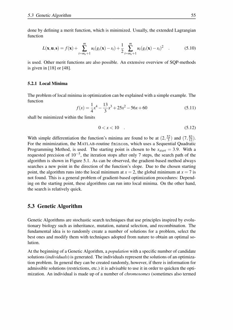
5.3 Genetic Algorithm 55
done by defining a merit function, which is minimized. Usually, the extended Lagrangianfunction
L(x,u,s) = f (x)+m
∑i=me+1
ui(gi(x)− si)+12
m
∑i=me+1
ui(gi(x)− si)2 . (5.10)
is used. Other merit functions are also possible. An extensive overview of SQP-methodsis given in [18] or [48].
5.2.1 Local Minima
The problem of local minima in optimization can be explained with a simple example. Thefunction
f (x) =14
x4− 133
x3 +25x2−56x+60 (5.11)
shall be minimized within the limits
0 < x < 10 . (5.12)
With simple differentiation the function’s minima are found to be at (2, 523 ) and (7, 83
12).For the minimization, the MATLAB-routine fmincon, which uses a Sequential QuadraticProgramming Method, is used. The starting point is chosen to be xstart = 3.9. With arequested precision of 10−5, the iteration stops after only 7 steps, the search path of thealgorithm is shown in Figure 5.1. As can be observed, the gradient-based method alwayssearches a new point in the direction of the function’s slope. Due to the chosen startingpoint, the algorithm runs into the local minimum at x = 2, the global minimum at x = 7 isnot found. This is a general problem of gradient-based optimization procedures: Depend-ing on the starting point, these algorithms can run into local minima. On the other hand,the search is relatively quick.
5.3 Genetic Algorithm
Genetic Algorithms are stochastic search techniques that use principles inspired by evolu-tionary biology such as inheritance, mutation, natural selection, and recombination. Thefundamental idea is to randomly create a number of solutions for a problem, select thebest ones and modify them with techniques adopted from nature to obtain an optimal so-lution.
At the beginning of a Genetic Algorithm, a population with a specific number of candidatesolutions (individuals) is generated. The individuals represent the solutions of an optimiza-tion problem. In general they can be created randomly, however, if there is information foradmissible solutions (restrictions, etc.) it is advisable to use it in order to quicken the opti-mization. An individual is made up of a number of chromosomes (sometimes also termed

56 5 Optimization
0
20
40
60
80
0 2 4 6 8 10
f(x)
x
Figure 5.1: Local minimum of SQP optimization
genomes) which represent a particular aspect of the solution. One common approach isto encode solutions as binary strings with each chromosome containing either 1 or 0 (seeFigure 5.2). The binary code can represent integers or real-valued parameters of the so-
0 1 101100100110100111101
One aspect of solution
Figure 5.2: Binary coded individual
lution. Another, similar approach is to encode solutions directly with integers or decimalnumbers (one number = one chromosome). This coding can often be ’intuitively closer tothe problem space’ [16].
After the creation of the first population, each individual is evaluated according to a fitnessfunction, i.e., for every individual, a fitness value is calculated which rates the ’quality’ ofthe individual. For a minimization problem, a very low fitness value reflects a good quality,whereas for a maximization problem it reflects a poor quality. Next, the population issorted by the fitness value - the individual with the best fitness takes in first place, followedby the second-best and so on. A number n of the poorest individuals are usually eradicated(survival of the fittest), these individuals are not allowed to produce offspring while thebetter ones constitute the parent population for the next generation. The forming of theoffspring generation is done using any or all of the genetic operators:

5.3 Genetic Algorithm 57
• Selectionindividuals are chosen for later breeding. Common procedures for selection are:
– Proportional fitnessan individuals chance to reproduce is proportional to its fitness value
– Tournament selectionrandomly selected individuals in a subgroup compete and the fittest one is se-lected
• Recombinationselected individuals are recombined. Usually, chromosome exchange and crossoverare used:
– Chromosome exchangebetween two individuals, the m-th chromosome is exchanged with a probabilityqce.
– One-point-crossoverwith a probability qco, two selected individuals exchange chromosome groupsfrom a specific chromosome position A to the end (see Figure 5.3).
1 0 1 011010011110 0 1 1 0 0 0 1 1
1 0 1 10110010011010011110
1 0 0 0 1 1 0 0 1 0 1 0 0 1 0 0 1 1 0 0 0 1 1
1 0 0 0 1 1 0 0 1 0 1 0 0 1 0 10110010
Figure 5.3: One-point-crossover
– Two-point-crossoverwith a probability qco, two selected individuals exchange chromosome groupsfrom a specific position A to a position B (see Figure 5.4).
• MutationThe value of a chromosome is mutated with a probability pmu, thus, for a binary-coded individual one chromosome value is changed from 1 to 0 or vice-versa (seeFigure 5.5).
Next to the individuals that are generated by recombination or mutation, also newly cre-ated individuals can be added to the new generation or the best individuals of the parentgeneration are left unchanged and added to the new generation (elite selection strategy).Once the new population is created, one iteration step is completed and the new individuals

58 5 Optimization
1 0
1 0 1 10110010011010011110
1 0 0 0 1 1 0 0 1 0 1 0 0 1 0 0 1 1 0 0 0 1 1
1 0 1 10110010010
1 0 0 0 1 1 0 0 1 1 0 0 0 1 1
1 0 0 1 0 1 0 0 1
11010011
Figure 5.4: Two-point-crossover
1 0 1 10110010011010011110
1 0 1 101100100101011111 0 1 0 0
Figure 5.5: Mutation
are evaluated and used to create the following generation. The iteration is halted if a spe-cific number of iterations is exceeded or if the best individual of a generation has reacheda specific fitness. Figure 5.6 shows the above described steps in a flowchart.
initialpopulation
recom−bination
newpopulation
new individuals
terminate?evaluation
yes
nomutation
Figure 5.6: Genetic algorithm
Genetic algorithms are often applied as an approach to solve global optimization prob-lems. They are in particular useful in problem domains that have a complex fitness land-scape as recombination is designed to move the population away from local minima thata traditional gradient-based algorithm might run into. There exist many different forms ofGenetic Algorithms and the user usually has to set a broad range of parameters.

5.4 Neural Network 59
5.4 Neural Network
Neural networks are composed of simple elements, neurons, operating in parallel. Thenetwork function is determined primarily by the connections between the neurons. Theseconnections are adjusted or weighted during a training or learning phase so that a particularinput leads to a specific output. When the training is finished, the adjusted network canbe used to solve a problem. See Figure 5.7 for the training of the Neural Network. The
inputdata
compareoutput target
calculate outputwith neural network
targetdata
adjustweights satisfactory?
output yesno terminate
Figure 5.7: Training of Neural Network
training phase is much more time-consuming than the actual application, which makes aneural network particularly suitable for real-time applications.
Neural networks are inspired from nature. The human brain consists of a large number ofneurons which perform a simple ’calculation’ and give their output to other neurons. Thebiological neurons are ’adjusted’ (trained) and act in a parallel manner. Figure 5.8 is aschematic drawing of a Neural Network that consists of an input layer, a hidden layer andan output layer. The input layer consists of nin neurons, corresponding to one set of inputdata with nin elements. The number of neurons in the hidden layer can be chosen somewhatarbitrarily. Theoretically, it is possible to construct a Neural Network with more than onehidden layer although most applications feature only a single hidden layer. The outputlayer consists of nout neurons, corresponding to an output data set with nout elements.
The neurons of the layers have weighted connections among each other. Thus, one neuronof the hidden layer has nin weighted inputs, as can be seen in Figure 5.9. The output of theneuron is calculated via
a21 = f 1(n) , (5.13)
where n is the sum of all outputs of the input layer
n =nin
∑i=1
ai ·w1,i +b , (5.14)
f is a transfer function and b is a bias. Typical choices for f are the sigmoid functionf = 1/(1+e−x) or the tangens hyperbolicus function. The transfer function f is employedfor the network to be able to identify nonlinear interrelationships.

60 5 Optimization
. . . .
. . . .
. . . .
neurons
input layer
hidden layer
output layer
weighted connections
a01 a0
2 a03 a0
4
a11 a1
2 a13
a21 a2
2
w11,1
w11,2
w21,1
w21,2
Figure 5.8: Neural Network with one hidden layer
Σ fn a1
b
w11,1
nin
Figure 5.9: Single neuron

5.4 Neural Network 61
The training of the Neural Network can be done using the backpropagation algorithm. Thesummary of the technique is as follows:
• Present a training sample to the Neural Network.
• Compare the network’s output to the desired output from that sample. Calculate theerror in each output neuron.
• For each neuron, calculate what the output should have been, and a scaling factor,how much lower or higher the output must be adjusted to match the desired output.
• Adjust the weights of each neuron to lower the local error.
• Repeat the steps above on the neurons at the previous level.
The training is finished if certain criteria are fulfilled, for example if a specific error tol-erance is reached or if the number of iterations exceeds a given value. As the algorithm’sname implies, the errors (and therefore the learning) propagate backwards from the outputnodes to the inner nodes. So backpropagation is used to change the network’s modifiableweight accordingly to the error.
The advantage of a Neural Network is the very quick application. After the very time-consuming training, the application of the Network is much quicker than other optimiza-tion procedures.

62 5 Optimization

6 EFFECTIVE PROPERTIES IN STATICS
The surface average based homogenization strategy proposed in section 4.2.4 is now real-ized in the static case using the optimization techniques given in chapter 5. Since in statics,an analytic solution of the homogenization problem is possible, the analysis is mainly doneto test the different optimization procedures with respect to what they can accomplish andwhat advantages and disadvantages they have. The following example calculations aredone in the two-dimensional case, the generalization to the 3-D case is possible withoutfurther considerations. Firstly, a number of beam-type microstructures are examined. Sec-ondly, a plate is considered with a star-shaped hole.
6.1 Beam-type microstructures
In order to calculate effective properties of a material, the components Qi jkl of the linearelastic constitutive equation have to be determined. The plane stress case is considered onthe macroscopic scale, so the 6 distinct Qi jkl of σ11
σ22σ12
=
Q1111 Q1122 Q1112Q2211 Q2222 Q2212Q1211 Q1222 Q1212
ε11ε22ε12
(6.1)
are sought.
Three different unit cells (see Figure 6.1) are used for the numerical study. The cell wallsconsist of steel with a Young’s modulus of E = 2.1× 10¹¹N/m2 and a quadratic cross-
0.25`
0.25`
0.5`
0.2`0.1`0.2`
0.5`
0.1`0.2`
0.2`
0.5`
Figure 6.1: Microstructures for numerical study
section of A = 10−8m2. The unit cells are calculated with the boundary element formu-lation described in chapter 3. In the static case, a Finite Element formulation could have
63

64 6 Effective properties in statics
been applied as well because a FEM calculation with shape functions of order three (e.g.Hermite-polynomials) gives exact results in the static case. The unit cells are subjectedto the three independent load cases shown in section 4.2.4 (see Figure 4.5). As boundaryconditions, the deformation at the boundary points are prescribed and the forces at thesepoints are calculated. Thus, as a result on the microscale, a set of stresses (σ11,σ22,σ12)and strains (ε11,ε22,ε12) is obtained for each loadcase.
After the calculation on the microscale, an optimization procedure is used to obtain ad-equate material parameters Qi jkl of equation (6.1). The optimization is formulated as aminimization problem, i.e., certain parameters need to be found to minimize a target func-tion. An optimal solution is found if the function value is 0. As target function, the meansquare error between the stress on micro- and macroscale is used
f =3
∑n=1
(σ
micro11 n −σ
macro11 n
)2+(σ
micro22 n −σ
macro22 n
)2+(σ
micro12 n −σ
macro12 n
)2. (6.2)
In equation (6.2), n denotes the loadcase, so the difference of stress is summed up overall three loadcases. The stress components on the microscale σmicro
i j n have to be calculatedonly once – with respect to the optimization they are constant input data. The stress onthe macroscopic scale σmacro
i j n , however, is calculated repeatedly for different Qi jkl in thecourse of the optimization via equation (6.1).
In the following sections, results are presented for the four different optimization strate-gies.
Genetic Algorithm
Each individual of a Genetic Algorithm has a fitness value which reflects the individualsquality. The fitness value is calculated from a fitness function which in the present caseis the target function f in equation (6.2). The material parameters Qi jkl represent thechromosomes of the individuals. There are a total of 9 Qi jkl , however, due to the symmetry,6 of them are independent. Therefore, each individual consists of 6 chromosomes.
A Genetic Algorithm has a broad range of parameters that need to be set. Parameterssuch as population size or type of genetic operators need to be chosen. For the presentapplication, the following parameters were used:
• A population size of 100 individuals is chosen
• The starting population is created randomly
• New individuals are created via 2-point-crossover
• The mutation of an individual is done accordingly to the standardized normal distri-bution
• 50 individuals are created newly in one generation, the remaining 50 are created asoffspring of the previous generation

6.1 Beam-type microstructures 65
• The optimization is stopped after a maximum of 500 iterations or if the best fitnessvalue is smaller than 10−5
These parameters were determined in a trial-and-error process and have shown to delivergood results. Figure 6.2 shows the performance of the Genetic Algorithm. The fitness
0
5000
10000
15000
20000
25000
0 50 100 150 200 250 300 350 400 450 500
fitne
ss v
alue
f
generation
optimization (1)optimization (2)optimization (3)
Figure 6.2: Performance of Genetic Algorithm
value of the best individual of a generation is plotted versus the number of generations. Theplot is done for the star-shaped cell on the right hand side of Figure 6.1. Since the startingpopulation is generated randomly, three optimization runs were done. At the beginning ofthe optimization, the progress of the algorithm is good, but after 40−50 generations, theimprovement of the fitness value is rather small. The sought material parameters were allfound with the Genetic Algorithm, see Table 6.1. The deviation from the exact solutionis given in Table 6.2. The exact solution can be calculated by solving the constitutiveequation (6.1) for the sought Qi jkl . This is done for the three independent loadcases. Inthe first loadcase, for example, only the strain ε11 is not equal to 0, so the correspondingequation is σ11
σ22σ12
=
Q1111 Q1122 Q1112Q2211 Q2222 Q2212Q1211 Q1222 Q1212
ε11ε22 = 0ε12 = 0
. (6.3)
Equation (6.3) can be solved for Q1111, Q2211 and Q1211.

66 6 Effective properties in statics
Neural Network
A Neural Network is now used to determine effective properties of the given microstruc-tures. In a first step, a Neural Network needs to be created and trained to solve the givenproblem.
Training of Neural Network
For the training, adequate examples must be given and on the basis of these examples, thenetwork is trained. One training example consists of the following components:
• Learning dataThe three loadcases given in Figure 4.5 are used with only one strain componentnot equal to 0 at a time. For each loadcase (given εi j), the corresponding stressis calculated using equation (6.1). The resulting 9 values (3 loadcases × 3 stresscomponents) for the stress form one set of learning data.
• Learning targetsThe learning targets consist of the 6 Qi jkl which had to be chosen in equation (6.1)to generate the learning data. The Qi jkl are chosen somewhat arbitrarily, however, itis meaningful to systematically cover a certain admissible range.
The choice of training examples is very important. For example, if the sought values forQi jkl lie outside the range of the training examples, the Neural Network can not be trainedproperly and will deliver poor results. In the present application, the choice of trainingexamples is difficult since à priori, no prediction can be made whether a component Qi jklhas the value 1 or 106.
Training: calculations with equation (6.1)
learning data
σ11, σ22, σ12 (LF 1)σ11, σ22, σ12 (LF 2)σ11, σ22, σ12 (LF 3)
...
←→
targets
Q1111 Q2222Q1122 Q1112Q2212 Q1212
...
1 set oflearningdata
n6 setsoflearningdata
Figure 6.3: Training data of Neural Network
Figure 6.3 shows the data for the training of the Neural Network. Another problem is thefact that chosen values for Qi jkl have to be combined among each other. If n differentvalues for one component are chosen, all combinations for the other 5 components mustbe made. Thus, the whole training set consists of n6 examples, so the training becomesvery extensive.

6.1 Beam-type microstructures 67
For the present application, the following parameters for the training of the Neural Networkhave proved to deliver good results:
• A backpropagation network is used with one hidden layer.
• In the training phase, 3 different values for the components Qi jkl are used. With 6independent Qi jkl , there are a total of 36 = 729 combinations.
• As transfer functions, linear functions are used.
The backpropagation method is used to determine the weights of the neurons. In Figure6.4, three typical training runs are shown. For the initial weights, random numbers were
1e-10
1e-08
1e-06
1e-04
0.01
1
0 50 100 150 200
mea
n sq
uare
erro
r
epochs
training run (1)training run (2)training run (3)
Figure 6.4: Training of Neural Network
chosen, so the training was different in the three runs.
Application of Neural Network
After the training of the Neural Network, it is applied to the parameter identification. Theunit cells are subjected to the three independent load cases shown in Figure 4.5. Theresulting 9 stress values are the input data for the Neural Network. The output of theNeural Network, of course, consists of the 6 unknown Qi jkl (see Figure 6.5). The soughtmaterial parameters were found, see Table 6.1. The deviation from the exact solution isgiven in Table 6.2.
Simplex Algorithm
The Simplex Algorithm uses an optimization function f (x) with n independent variables(x = x1,x2, ...xn). Equation (6.2) is used here for the homogenization. The six independent

68 6 Effective properties in statics
Application of Neural Network: Calculation on Unit Cell
input data
σ11, σ22, σ12 (lc 1)σ11, σ22, σ12 (lc 2)σ11, σ22, σ12 (lc 3)
←→
sought parameters
Q1111 = ? Q2222 = ?Q1122 = ? Q1112 = ?Q2212 = ? Q1212 = ?
1 set ofdata
Figure 6.5: Data for application of Neural Network
Qi jkl are the sought variables of the optimization function. The function nag_opt_simplex(e04ccc) of the NAG-library [50] was used for the implementation. The following param-eters were used:
• Random values are used as starting points
• The optimization stops if f < 10−5 or a maximum of 10000 iterations is reached
• Formulation as unconstrained problem, i.e., no constraints for values of Qi jkl aremade
Figure 6.6 shows typical optimization runs. The mean square error is plotted versus the
-1e+08
0
1e+08
2e+08
3e+08
4e+08
5e+08
6e+08
7e+08
8e+08
0 500 1000 1500 2000 2500 3000 3500
mea
n sq
uare
err
or
iterations
optimization (1)optimization (2)optimization (3)
Figure 6.6: Optimization with Simplex algorithm
number of iterations. A comparatively large number of iterations is needed until an accept-able value for the mean square error is reached. However, one iteration step only needs

6.1 Beam-type microstructures 69
a little computing time. The sought material parameters were found with the SimplexAlgorithm, see Table 6.1.
SQP: Sequential Quadratic Programming
Analogously to the Simplex Algorithm, equation (6.2) is used as optimization functionfor the Sequential Quadratic Programming method. The method does not only need theoptimization function itself, but also the first derivatives of it. Equation (6.2) can be dif-ferentiated with respect to the 6 Qi jkl , so no numerical procedures like Finite Differenceshave to be used. The function nag_opt_nlin_sqp (e04unc) of the NAG-library was usedfor the implementation. The following parameters were used:
• Random values are used as starting points
• The optimization stops if f < 10−5 or a maximum of 10000 iterations is reached
• Formulation as unconstrained problem, i.e., no constraints for values of Qi jkl aremade
Figure 6.7 shows typical optimization runs. The mean square error is plotted versus the
0
5000
10000
15000
20000
0 1 2 3 4 5
mea
n sq
uare
err
or
iterations
optimization (1)optimization (2)optimization (3)
Figure 6.7: Optimization with SQP method
number of iterations. Since the derivatives of the optimization function (6.2) are used,the SQP method only needs very few iteration steps until the postulated value for the

70 6 Effective properties in statics
mean square error is reached. The sought material parameters were found with the SQPalgorithm, see Table 6.1.
Discussion of results
The calculation of effective parameters of the 3 given microstructures was successfullyaccomplished by all optimization procedures. The calculated parameters are given in Table6.1. The correctness of the found Qi jkl were verified using equation (6.1). Due to the
microstructure (1)
Gen. Alg. Neur. Net Simplex SQP
Q1111 8.3307 ·102 8.3307 ·102 8.3307 ·102 8.3307 ·102
Q1122 4.9789 ·102 4.9789 ·102 4.9789 ·102 4.9789 ·102
Q1112 1.6636 ·10−7 −4.0000 ·10−10 −4.9000 ·10−10 −2.2205 ·10−19
Q2222 8.3307 ·102 8.3307 ·102 8.3307 ·102 8.3307 ·102
Q2212 1.0595 ·10−7 −1.0720 ·10−7 −1.3000 ·10−10 −4.4409 ·10−19
Q1212 3.0141 ·10−3 3.0150 ·10−3 3.0150 ·10−3 3.0150 ·10−3
microstructure (2)Gen. Alg. Neur. Net Simplex SQP
Q1111 4.1349 ·102 4.1349 ·102 4.1349 ·102 4.1349 ·102
Q1122 −3.2750 ·10−1 −3.2750 ·10−1 −3.2750 ·10−1 −3.2750 ·10−1
Q1112 −5.6623 ·10−8 2.2500 ·10−8 −1.0000 ·10−11 −4.4409 ·10−19
Q2222 4.1349 ·102 4.1349 ·102 4.1349 ·102 4.1349 ·102
Q2212 −5.0256 ·10−8 −1.2300 ·10−8 −2.1000 ·10−10 8.8818 ·10−19
Q1212 1.5120 ·10−3 1.5119 ·10−3 1.5119 ·10−3 1.5119 ·10−3
microstructure (3)Gen. Alg. Neur. Net Simplex SQP
Q1111 2.1149 ·102 2.1149 ·102 2.1149 ·102 2.1149 ·102
Q1122 −8.1308 ·101 −8.1308 ·101 −8.1308 ·101 −8.1308 ·101
Q1112 3.9604 ·10−8 −5.0000 ·10−10 8.0000 ·10−11 −5.4210 ·10−23
Q2222 2.1149 ·102 2.1149 ·102 2.1149 ·102 2.1149 ·102
Q2212 2.1499 ·10−8 1.0000 ·10−9 −2.4000 ·10−10 4.3368 ·10−22
Q1212 1.5119 ·10−3 1.5119 ·10−3 1.5119 ·10−3 1.5119 ·10−3
Table 6.1: Results of optimization

6.1 Beam-type microstructures 71
symmetry of the unit cells, the components Q1111 and Q2222 are always equal, i.e., thestiffness in horizontal and vertical direction is the same. Moreover, the components Q1112and Q2212 are always 0.
microstructure (1)
exact solution Gen. Alg. Neur. Net Simplex SQP
Q1111 8.3307·102 - - - -Q1122 4.9789·102 - - - -Q1112 0 < 10−6 < 10−9 < 10−9 < 10−18
Q2222 8.3307·102 - - - -Q2212 0 < 10−6 < 10−6 < 10−9 < 10−18
Q1212 3.0150·10−3 < 10−6 - - -
microstructure (2)
exact solution Gen. Alg. Neur. Net Simplex SQP
Q1111 4.1349·102 - - - -Q1122 −3.2750·10−1 - - - -Q1112 0 < 10−7 < 10−7 < 10−10 < 10−18
Q2222 4.1349·102 - - - -Q2212 0 < 10−7 < 10−7 < 10−9 < 10−18
Q1212 1.5119·10−3 < 10−6 - - -
microstructure (3)
exact solution Gen. Alg. Neur. Net Simplex SQP
Q1111 2.1149·102 - - - -Q1122 −8.1308·101 - - - -Q1112 0 < 10−7 < 10−9 < 10−10 < 10−22
Q2222 2.1149·102 - - - -Q2212 0 < 10−7 < 10−8 < 10−9 < 10−21
Q1212 1.5119·10−3 - - - -
Table 6.2: Results of optimization: deviation from exact solution
As expected, all optimization procedures have determined the sought material parameterscorrectly. Since numerical procedures were used, the solutions are only correct to a certainprecision. Therefore, the components Q1112 and Q2212 are not exactly 0.
The numerical cost to obtain a solution was quite different. The Simplex method, whichis the least complicated of all procedures, needed a large number of (quick) iterations. Incomparison to that, the SQP method was much faster, which is logical because the first

72 6 Effective properties in statics
derivatives of the optimization function is used by the method. Thus, more informationabout the problem is given to the algorithm, resulting in a significant improvement inperformance. The Genetic Algorithm also delivered good results, although it was not asquick as the SQP method.
The Neural Network was, compared to the first three procedures, rather difficult to usefor the given problem. Firstly, the training of the Network is numerically very expensive.Secondly, it is hard to find suitable training examples. The number of training examplesincreases rapidly the more values for the single components Qi jkl are used because allcombinations of the components have to be made. However, once the training is completethe Neural Network delivers good, quick results. It depends on the intended applicationwhether the use of a Neural Network is meaningful: If the computation of parametersneeds to be done for a lot of different microstructures, it makes sense to train a NeuralNetwork once and then apply it many times. On the other hand, if only a single compu-tation of material parameters is needed, the other optimization procedures are definitelymore suitable.
6.2 Plane stress microstructure
The calculation of effective static properties is now done for a plate in plane stress. Themicrostructure given in Figure 6.8 is considered. The calculation of the plate is done with
20 elements
10 elements0.12`
0.28`
0.1`
`
Figure 6.8: Microstructure for numerical study
the Boudary Element Method, a discretization of 20 elements on the outer edges and 10

6.2 Plane stress microstructure 73
elements on one part of the inner edge according to Figure 6.8 is used. The material of theplate is steel with a Young’s modulus of E = 2.1×10¹¹N/m2 and a Poisson’s ratio of 0.3.The plate is loaded with a prescribed displacement of 0.05` on the left and right hand side,while the upper and lower edges can deform freely, see Figure 6.9. These homogeneous
u = 0.05` u = 0.05`
Figure 6.9: Loadcase of microstructure
boundary conditions do not fulfill the periodicity conditions, because neighbouring cellsdo not undergo the same deformation pattern. This is neglected, however, because boththe deformation and the tractions on the cell edges are averaged. Thus, after the averagingprocess, periodicity is fulfilled. The averaging is pictured in Figure 6.10. With this, analo-
undeformed deformed uavg
σavg
Figure 6.10: Averaging of deformation and tractions
gously to the beam-type microstructures, a set of averaged stresses and strains is obtained.In the present case, only the stress σmicro
11 and the strains εmicro11 and εmicro
22 are not equal to0
σmicro11 6= 0, ε
micro11 6= 0, ε
micro11 6= 0 (6.4)
σmicro22 = 0, σ
micro12 = 0, ε
micro12 = 0 . (6.5)
These stresses and strains are the input data for the optimization process, where effectiveproperties are calculated. On the macroscopic scale, the constitutive equation
σmacroi j =
E(1+ν)
εmacroi j +
νE(1+ν)(1−2ν)
δi j εmacrokk (6.6)
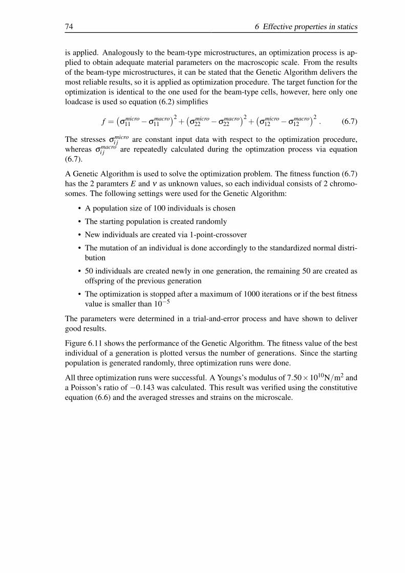
74 6 Effective properties in statics
is applied. Analogously to the beam-type microstructures, an optimization process is ap-plied to obtain adequate material parameters on the macroscopic scale. From the resultsof the beam-type microstructures, it can be stated that the Genetic Algorithm delivers themost reliable results, so it is applied as optimization procedure. The target function for theoptimization is identical to the one used for the beam-type cells, however, here only oneloadcase is used so equation (6.2) simplifies
f =(σ
micro11 −σ
macro11
)2+(σ
micro22 −σ
macro22
)2+(σ
micro12 −σ
macro12
)2. (6.7)
The stresses σmicroi j are constant input data with respect to the optimization procedure,
whereas σmacroi j are repeatedly calculated during the optimzation process via equation
(6.7).
A Genetic Algorithm is used to solve the optimization problem. The fitness function (6.7)has the 2 paramters E and ν as unknown values, so each individual consists of 2 chromo-somes. The following settings were used for the Genetic Algorithm:
• A population size of 100 individuals is chosen
• The starting population is created randomly
• New individuals are created via 1-point-crossover
• The mutation of an individual is done accordingly to the standardized normal distri-bution
• 50 individuals are created newly in one generation, the remaining 50 are created asoffspring of the previous generation
• The optimization is stopped after a maximum of 1000 iterations or if the best fitnessvalue is smaller than 10−5
The parameters were determined in a trial-and-error process and have shown to delivergood results.
Figure 6.11 shows the performance of the Genetic Algorithm. The fitness value of the bestindividual of a generation is plotted versus the number of generations. Since the startingpopulation is generated randomly, three optimization runs were done.
All three optimization runs were successful. A Youngs’s modulus of 7.50×10¹⁰N/m2 anda Poisson’s ratio of −0.143 was calculated. This result was verified using the constitutiveequation (6.6) and the averaged stresses and strains on the microscale.

6.2 Plane stress microstructure 75
0
2e+06
4e+06
6e+06
8e+06
1e+07
0 100 200 300 400 500 600 700 800 900 1000
fitne
ss v
alue
f
generation
optimization (1)optimization (2)optimization (3)
Figure 6.11: Performance of Genetic Algorithm

76 6 Effective properties in statics

7 EFFECTIVE PROPERTIES IN DYNAMICS
In this chapter, the prescribed homogenization strategy is realized in the dynamic case, i.e.,the microstructure is calculated in frequency domain with a harmonic excitation. Due toinertia, the response of the unit cell is frequency dependent: if a harmonic stress is given,the strain is frequency dependent and vice-versa. The frequency dependence is also givenon the macroscopic scale, thus, a frequency dependent macroscopic constitutive equationis required. Here, a viscoelastic constitutive equation is chosen on the macroscale.
In statics, it has been shown that the homogenization problem can be solved analytically.The stress and strain can be calculated and the constitutive equation can be solved for theunknown material parameters. The same can be done in frequency domain as well, butonly if one specific frequency ω is considered at a time. It is possible to calculate stressand strain for an excitation frequency ω and obtain material parameters for this frequency.This can be done repeatedly, so material parameters for a number of frequencies can becomputed. However, it is desirable to not only have material parameters for a specificfrequency but for a whole frequency range. Thus, the aim is to obtain parameters of aconsitutive equation like
σ(ω) =
N∑
k=0qk(iω)k
N∑
k=0pk(iω)k
ε(ω) , (7.1)
see also equation (2.57). pk and qk are parameters which cover a large frequency range. Toobtain adequate values for these parameters, it is necessary to calculate the stress σmicro(ω)and strain εmicro(ω) on the microscale for a number of frequencies, covering a specificrange. Either the stress is given and the strain is calculated or vice-versa. In the macro-scopic constitutive equation, e.g., equation (7.1) the parameters pk and qk have to be foundto correspond to the microscale results. For example, if a microscopic strain εmicro(ω)is prescribed, the frequency response σmicro(ω) must correspond to a macroscopic stressσmacro(ω), where σmacro(ω) is a function of the material parameters pk and qk, i.e.,
σmicro(ω) != σ
macro(ω, pk,qk) . (7.2)
To satisfy equation (7.2), the mean square error between stress on the micro- and macroscaleis taken and the difference is minimized(
σmicro(ω)−σ
macro(ω, pk,qk))2→ 0 . (7.3)
At this point, an optimization procedure is required. The parameters of the constitutiveequation must be chosen such that the difference between micro- and macroscale are as
77

78 7 Effective properties in dynamics
small as possible. Since the stress on the microscale can only be calculated for discretefrequencies the mean square error of equation (7.3) is summed up over a number of discretefrequency steps
f =ωend
∑ωstart
(σ
micro(ω)−σmacro(ω, pk,qk)
)2→ 0 . (7.4)
If a microscopic stress is given, the stress must be replaced by the strain in equations (7.3)and (7.4).
From the results in the static case, it can be stated that the Neural Network is not suitable tosolve the optimization problem. The reason is that in the training phase, training examplesmust be chosen with specific values for the sought material parameters. In order to covera range for pk and qk, a very large number of training examples would be necessary. Thus,only the gradient-based optimization procedures and the Genetic Algorithm are used forthe optimization.
The chapter consists of 3 parts. Firstly, effective properties are calculated within a smallfrequency range, i.e., from the static case (ω→ 0) up to the first eigenfrequency. Secondly,a broader frequency range is covered. For both frequency ranges, beam-type microstruc-tures are analyzed. In the last section, a plate in plane stress state is investigated.
7.1 Beam cells in small frequency range
The microstructure shown in Figure 7.1 is used for the following considerations. The cell
0.2`
0.1`0.2`
0.5`
u = u · e i ω t u = u · e i ω t
Figure 7.1: Geometry and load case of the unit cell
is analzed in frequency domain. A harmonic strain in one direction is applied to the cell(see also Figure 7.1). The procedure presented in chapter 2 is used for the calculationbecause it delivers exact results.
Since the considered microstructure is assumed to be periodic, the opposing nodes of thecell must have the same deformation and the forces of the node pairs must be equal in

7.1 Beam cells in small frequency range 79
magnitude but opposite in direction. Due to the symmetry of the cell periodicity is fulfilled,e.g., the reaction force of the node on the left hand side corresponds to the applied load onthe right hand side.
The cell consists of beams with a quadratic cross section of 0.1 ·`×0.1 ·`. The microstruc-ture material is steel with a Young’s modulus of E = 2.1 · 1011N/m2. The frequency re-sponse for an applied displacement amplitude of u = 0.001` is calculated on a logarithmicscale up to a frequency of 18 kHz.
On the macroscale, the one-dimensional constitutive equation
σ(ω) = G(iω) ε(ω) =
N∑
k=1qk(iω)k
M∑
k=1pk(iω)k
ε(ω) (7.5)
is used (see also equation (2.55)). Equation (7.5) has to be fulfilled for a frequency range0..ωmax. Contrary to the static (1-D) case, a larger number of parameters have to be de-termined. The number of parameters is somewhat arbitrary, it depends on the consideredfrequency range how many parameters have to be used. For the present case, it has turnedout that a total M +N = 14 parameters are sufficient to deliver good results for the consid-ered frequency range.
For the formulation of the homogenization problem as an optimization problem, the meansquare error technique is used. The square difference of the stress on micro- and macroscalemust be 0 for the optimal parameters on the macroscale
f =ωmax
∑ω=0
(σ
micro(ω)−σmacro(ω, pk,qk)
)2→ 0 . (7.6)
7.1.1 Genetic Algorithm
The fitness value of the individuals quality is calculated via equation (7.6). A total numberof M + N = 14 parameters is used, so each individual consists of 14 chromosomes. In atrial and error process, the following parameters of the Genetic Algorithm have shown tobe suitable for the present application:
• A population size of 1000 individuals is chosen
• The starting population is created randomly
• New individuals are created via 2-point-crossover
• The mutation of an individual is done accordingly to the standardized normal distri-bution
• 250 individuals are created newly in one generation, the remaining 750 are createdas offspring of the previous generation

80 7 Effective properties in dynamics
• The optimization is stopped after a maximum of 50000 iterations or if the best fitnessvalue f < 10−5.
The proceeding of the optimization is shown in Figure 7.2. Since the first generation iscreated randomly and also during the optimization, genetic operators are applied randomly,the proceeding of the optimization is different in all the optimization runs. The fitness value
0
5
10
15
20
25
30
35
40
45
0 10000 20000 30000 40000 50000
fitne
ss v
alue
f
generation
optimization (1)optimization (2)optimization (3)
Figure 7.2: Optimization with Genetic Algorithm
of the best individual is plotted versus the number of generations. It can be seen that inall three cases, a relatively small fitness values was obtained, however, after a differentnumber of generations. The obtained values for pk and qk are given in Table 7.1. Contraryto the static case, there is more than one set of parameters which describes the behavioraccurately. Figure 7.3 shows the behavior on the micro- and macroscale. The modulusG(ω) is plotted versus the frequency. On the microscale (solid line), G(ω) is
G(ω) =σmicro
εmicro (7.7)
with the stress and strain σmicro,εmicro of the unit cell, whereas for the three macroscaleresults, equation (7.5) was solved for ε(ω) and plotted for the three optimization runs withthe respective parameters pk and qk given in Table 7.1.
7.1.2 Simplex Algorithm
The Simplex Algorithm is used to determine the macroscale parameters. The optimizationfunction (7.5) with the 14 parameters is minimized. Like in the static case, the functionnag_opt_simplex (e04ccc) of the NAG-library was used with the following settings:

7.1 Beam cells in small frequency range 81
optimization (1) f = 0.02996
k qk pk
1 1.7617 ·101 1.5469 ·107
2 2.2672 ·102 1.8152 ·108
3 −1.7471 ·10−14 1.2785 ·105
4 1.8300 ·100 1.4790 ·106
5 3.3705 ·10−3 1.0693 ·104
6 4.2695 ·10−3 3.0166 ·103
7 1.7815 ·10−19 4.0734 ·101
optimization (2) f = 0.08141
k qk pk
1 4.9398 ·100 4.1763 ·106
2 4.0007 ·102 3.8899 ·108
3 −1.6224 ·10−14 4.3765 ·105
4 2.1568 ·100 2.7570 ·106
5 1.2825 ·10−16 6.7831 ·103
6 2.9828 ·10−3 4.8445 ·103
7 5.0153 ·10−5 2.0826 ·101
optimization (3) f = 0.02313
k qk pk
1 7.6350 ·10−5 6.3904 ·101
2 2.0017 ·102 1.6060 ·108
3 −7.0055 ·10−14 4.0609 ·105
4 1.1501 ·100 1.1117 ·106
5 4.4045 ·10−16 5.5493 ·103
6 1.7722 ·10−3 1.8973 ·103
7 2.6157 ·10−5 1.5891 ·101
Table 7.1: Obtained material parameters by Genetic Algorithm
0.01
0.1
1
10
100
0 2 4 6 8 10 12 14 16 18
G
frequency [kHz]
microscaleoptimization (1)optimization (2)optimization (3)
Figure 7.3: Genetic Algorithm results on the micro- and macroscale

82 7 Effective properties in dynamics
• Random values are used as starting points
• The optimization stops if f < 10−5 or a maximum of 10000 iterations is reached
• Formulation as unconstrained problem, i.e., no constraints for values of pk and qkare made.
The courses of three optimization runs are shown in Figure 7.4. The fitness value is plotted
0
20
40
60
80
100
0 2000 4000 6000 8000 10000
fitne
ss v
alue
f
iterations
optimization (1)optimization (2)optimization (3)
Figure 7.4: Optimization using Simplex algorithm
versus the number of iterations. As can be seen, the optimization did not end with anoptimal value close to 0 in all three runs. One optimization run found a local minimum ofthe optimization function, which is due to a ’wrong’ starting point. The calculated materialparameters and final values of the optimization function are given in Table 7.2.
Analogously to the Genetic Algorithm, Figure 7.5 shows the comparison of the micro-and macroscale. For the first and third optimization run, the micro- and macroscale resultsfit relatively well. The calculated parameters of the second run, however, show a ratherpoor fit, which could have already been expected from the final value of the optimizationfunction ( f = 40.36443).
7.1.3 SQP - Sequential Quadratic Programming
The Sequential Quadratic Programming method is used to minimize the optimization func-tion (7.6). The following parameters were used:
• Random values are used as starting points
• The optimization stops if f < 10−5 or a maximum of 1000 iterations is reached

7.1 Beam cells in small frequency range 83
optimization (3) f = 0.02313
k qk pk
1 −2.3120 ·10−1 8.7004 ·104
2 9.9885 ·102 9.9986 ·108
3 −6.3275 ·100 1.6585 ·106
4 3.8550 ·100 5.0101 ·105
5 2.2212 ·100 1.3758 ·106
6 8.6224 ·10−2 −1.2021 ·104
7 9.6364 ·10−3 5.3747 ·103
optimization (2) f = 4.03644
k qk pk
1 4.2969 ·100 4.6088 ·106
2 3.7837 ·100 −9.4540 ·106
3 −4.3263 ·101 −6.5015 ·106
4 2.0501 ·101 6.1724 ·106
5 −5.3712 ·101 −4.1837 ·106
6 −1.1843 ·101 1.6728 ·106
7 −7.7912 ·100 −1.8432 ·106
optimization (3) f = 0.08141
k qk pk
1 −1.2788 ·10−1 −8.1114 ·104
2 −2.4249 ·10−1 −3.2711 ·104
3 −1.7395 ·10−1 −3.9820 ·104
4 −4.3973 ·10−2 −2.8295 ·104
5 −1.0598 ·10−1 −3.9454 ·104
6 −4.0095 ·10−2 −1.1223 ·102
7 −3.0264 ·10−4 −1.5512 ·102
Table 7.2: Obtained material parameters by Simplex Algorithm
0.001
0.01
0.1
1
10
100
0 2 4 6 8 10 12 14 16 18
G
frequency [kHz]
microscaleoptimization (1)optimization (2)optimization (3)
Figure 7.5: Simplex results on the micro- and macroscale

84 7 Effective properties in dynamics
• Formulation as unconstrained problem, i.e., no constraints for values of pk and qkare made
Figure 7.6 shows typical optimization runs. The fitness value is plotted versus the number
0
20
40
60
80
100
0 200 400 600 800 1000
fitne
ss v
alue
f
iterations
optimization (1)optimization (2)optimization (3)
Figure 7.6: Optimization using SQP algorithm
of iterations. The SQP method was able to obtain a value f < 1 in two runs. One opti-mization run was only able to find a local minimum of the function. This can be seen fromthe final value of the optimization of f = 31.2730 and also from the results for G(ω) onmicro- and macroscale. See Table 7.3 for the obtained values for the parameters pk and qkand Figure 7.6 for results on both scales.
7.1.4 Discussion of results
All three optimization procedures were able to find adequate material parameters on themacroscopic scale. It can already be seen from the fitness value or final value of the op-timization function, respectively, how good the parameters fit the microscopic properties.The Simplex Algorithm and the Sequential Quadratic Programming method both haveproblems with local minima. If a ’wrong’ starting point is used for the optimization, theymay deliver poor results. The Simplex Algorithm is much slower than the SQP method,which is obvious since it does not use the first derivatives of the optimization function. TheGenetic Algorithm is the most reliable of all optimization procedures. No starting pointis required, and it always delivers good results. However, it takes much more computingtime to obtain results.

7.1 Beam cells in small frequency range 85
optimization (1) f = 31.2730
k qk pk
1 2.3801 ·103 1.7790 ·106
2 −2.1948 ·104 2.9126 ·106
3 −3.5378 ·104 9.0371 ·104
4 −2.0615 ·104 −9.9309 ·105
5 −6.5232 ·103 −1.7844 ·102
6 −9.5146 ·102 5.9092 ·103
7 1.1842 ·104 1.2702 ·100
optimization (2) f = 0.0942
k qk pk
1 2.7349 ·108 2.3917 ·1011
2 −7.8132 ·108 −2.5963 ·1011
3 3.0370 ·108 −1.1559 ·1011
4 3.0801 ·108 −4.0479 ·1010
5 1.2956 ·108 7.1634 ·1010
6 −3.1951 ·106 −2.2324 ·108
7 4.4835 ·105 2.8131 ·108
optimization (3) f = 0.0961
k qk pk
1 −1.7145 ·10−1 −1.2534 ·102
2 −6.7364 ·10−1 −1.0430 ·102
3 −9.4824 ·10−1 4.1414 ·101
4 1.6859 ·100 1.8603 ·101
5 −1.8562 ·10−1 −1.0769 ·102
6 2.6000 ·10−5 −2.8079 ·10−2
7 −6.5400 ·10−4 −4.2114 ·10−1
Table 7.3: Obtained material parameters by SQP
0.01
0.1
1
10
100
0 2 4 6 8 10 12 14 16 18
G
frequency [kHz]
microscaleoptimization (1)optimization (2)optimization (3)
Figure 7.7: SQP results on the micro- and macroscale

86 7 Effective properties in dynamics
7.2 Beam cells in large frequency range
Effective properties for a broader frequency range are determined for both auxetic and non-auxetic microstructures in this chapter. The following two microstructures given in Figure7.8 are used for the numerical study. Both cells consist of beams with a quadratic cross
0.2`
0.1`0.2`
0.5`
0.2`
0.3`
0.5`
Figure 7.8: Auxetic and non-auxetic microstructures
section of 0.1`× 0.1`. The microstructure material is PMMA with a slight damping (seeAppendix D). A frequency range from 0 up to 3×10³ kHz is chosen. Due to the existenceof higher eigenmodes for more than one unit cell (see section 4.2.5), the microstructuresare calculated multiple times. Calculations were done for 1, 2×2, ...n×n unit cells up ton = 5 and the results were averaged. The loadcase for both cells is given in Figure 7.9.Again, a displacement amplitude is applied on the left and right hand side of the cell.
u = u · e i ω t u = u · e i ω t
Figure 7.9: Loadcase
On the macroscale, the constitutive equation
σi j(ω) =E(ω)
(1+ν(ω))εi j(ω)+
ν(ω)E(ω)(1+ν(ω))(1−2ν(ω))
δi j εkk(ω) (7.8)
is applied. For Young’s modulus, the viscoelastic model
E(ω) = E1+q1(iω)α1 +q2(iω)α2
1+ p1(iω)α1 + p2(iω)α2. (7.9)
with fractional derivatives and 7 parameters is used. The same model but with possibledifferent parameters is used for Poisson’s ratio
ν(ω) = ν1+ q1(iω)α1 + q2(iω)α2
1+ p1(iω)α1 + p2(iω)α2. (7.10)

7.2 Beam cells in large frequency range 87
Again, the choice of these models is somewhat arbitrary. For the considered frequencyrange, they have shown to be sufficient. A number of trials with fewer parameters were notsuccessful, as well as models with more parameters, yet without fractional derivatives.
From the results of the previous chapter, it can be stated that the Genetic Algorithm isthe most reliable optimization procedure to obtain the sought material parameter. Thegradient-based optimization techniques were quicker, however, the results are not reliable.Thus, a Genetic Algorithm is applied here. The following parameters were used to deter-mine the material parameters:
• A population size of 1000 individuals is chosen
• The starting population is created randomly
• New individuals are created via 2-point-crossover
• The mutation of an individual is done accordingly to the standardized normal distri-bution, mutation probability is 10%
• 150 individuals are created newly in one generation, the remaining 850 are createdas offspring of the previous generation
• The optimization is stopped after a maximum of 50000 iterations or if the best fitnessvalue f < 10−5.
The results of the optimization are depicted in the following Figures. Figures 7.10 and7.11 show the Young’s modulus and Poisson’s ratio for the auxetic microstructure, whilein Figures 7.12 and 7.13, Young’s modulus and Poisson’s ratio for the non-auxetic mi-crostructure are shown. In each diagram, the microscopic and macroscopic results areplotted versus the frequency.
As can be seen, the optimization was not able to fit each single eigenfrequency of themicrostructure results. However, the general tendency is preserved. In all four result plots,it can be seen that for small frequencies, the fitted parameters converge into the staticsolution. The obtained material parameters for ν and E are given in Table 7.4 for theauxetic microstructure and in Table 7.5 for the non-auxetic material.
The slightly viscoelastic material on the microscopic scale had virtually no effect on thehomogenization process. There were still eigenfrequencies on the microscale which causethat the search of the material parameters is very difficult.
For the optimization, it can be observed that there is no difference whether an auxetic ornon-auxetic microstructure is used as input data. This could have been expected à priori,because the same mathematical problem (with slightly different parameters) needs to besolved by the optimization procedure.

88 7 Effective properties in dynamics
1000
10000
100000
1e+06
1e+07
1e+08
10 100 1000
microscalemacroscale
E[N
/m
2 ]
frequency [kHz]
Figure 7.10: Young’s modulus for auxetic microstructure
-1
-0.5
0
0.5
1
10 100 1000
microscalemacroscale
ν[−
]
frequency [kHz]
Figure 7.11: Poisson’s ratio for auxetic microstructure

7.2 Beam cells in large frequency range 89
1000
10000
100000
1e+06
1e+07
1e+08
10 100 1000
microscalemacroscale
E[N
/m
2 ]
frequency [kHz]
Figure 7.12: Young’s modulus for non-auxetic microstructure
-1
-0.5
0
0.5
1
10 100 1000
microscalemacroscale
ν[−
]
frequency [kHz]
Figure 7.13: Poisson’s ratio for non-auxetic microstructure

90 7 Effective properties in dynamics
Young’s modulus
k E pk qk αk
1 2.560 ·104 2.358 ·10−6 1.842 ·10−8 1.057 ·100
2 2.432 ·10−8 1.448 ·10−12 1.099 ·100
Poisson’s ratio
k ν pk qk αk
1 −0.376 4.995 ·10−8 1.598 ·10−8 1.497 ·100
2 1.534 ·10−8 1.162 ·10−7 1.335 ·100
Table 7.4: Obtained material parameters for auxetic material
Young’s modulus
k E pk qk αk
1 1.581 ·105 1.057 ·10−6 2.666 ·10−8 1.057 ·100
2 1.448 ·10−12 1.856 ·10−8 1.389 ·100
Poisson’s ratio
k ν pk qk αk
1 0.307 1.869 ·10−11 1.407 ·10−8 1.424 ·100
2 5.147 ·10−9 8.443 ·10−10 1.573 ·100
Table 7.5: Obtained material parameters for non-auxetic material

7.3 Plate cells 91
7.3 Plate cells
Until here, a number of beam-type examples were presented in dynamics. In addtion tothat, a plate in plane stress is now investigated. The same geometry as in section 6.2 isused. For comparison, a plate without a hole is calculated. The discretization of the platesare given in Figure 7.14. Again, the Boundary Element Method is used for the calculationso that only the edges of the structure have to be discretized. For the cell with the star-
20 elements
10 elements0.12`
0.28`
0.1`
` `
20 elements
Figure 7.14: Microstructures for numerical study
shaped hole, the same discretization as in statics is used with 20 elements on each of theouter edges and 10 elements on one part of the inner edge. The plate without hole onlyhas 20 elements on each outer edge. The loading of the cells is also done accordingly tosection 6.2, however, with a harmonic excitation on the left and right hand side (see Figure7.15). The material of the plate is steel with a Young’s modulus of E = 2.1× 10¹¹N/m2
u = 0.05 `eiω t uu u
` `
Figure 7.15: Loading of microstructures
and a Poisson’s ratio of 0.3.

92 7 Effective properties in dynamics
Just like in the previous considerations, a surface averaging of the stresses and strainsis done. With theses stresses and strains, Young’s modulus and Poisson’s ratio can becalculated on the microscale via the constitutive equation
σmicroi j (ω) =
E(ω)(1+ν(ω))
εmicroi j (ω)+
ν(ω)E(ω)(1+ν(ω))(1−2ν(ω))
δi j εmicrokk (ω) (7.11)
The next step to be done is, of course, to find adequate parameters for Young’s modulusand Poisson’s ratio on the macroscopic scale, e.g. parameters of viscoelastic models likethe ones calculated in section 7.2
E(ω) = E1+qk(iω)αk
1+ pk(iω)αkk = 1, ..,n (7.12)
ν(ω) = ν1+ qk(iω)αk
1+ pk(iω)αkk = 1, ..,n . (7.13)
However, the results of the microscale computation do not allow a computation of macro-scopic parameters like in case of the beam-type structures. In Figures 7.16 and 7.17, bothYoung’s modulus and Poisson’s ratio on the microscale are plotted versus the frequencyfor the two considered microstructures.
-1e+13
-5e+12
0
5e+12
1e+13
0 200 400 600 800 1000
E[N
/m
2 ]
frequency [Hz]
-2-1.5
-1-0.5
0 0.5
1 1.5
2
0 200 400 600 800 1000
ν[−
]
frequency [Hz]Figure 7.16: Young’s modulus and Poisson’s ratio on microscale for plate
It can be seen that E and ν converge to the static solution in the low frequencies. In thecase of the the plate without hole, Young’s modulus is E = 2.1×10¹¹N/m2 and Poisson’sratio is ν = 0.3 for frequencies close to 0, according to the input data of the plate. Theplate with the star-shaped hole converges into the static solution of E = 7.50×10¹⁰N/m2
and ν = −0.143 given in section 6.2. Thus, the frequency solution in the low frequencyrange is well confirmed.
In higher frequencies, however, all four plots expose a behavior which can not be usedfor a macroscopic material model. Contrary to the results of the beam-type cells, theresults do not show a general tendency, i.e., they do not lie in the vicinity of a specific

7.3 Plate cells 93
-1e+13
-5e+12
0
5e+12
1e+13
0 200 400 600 800 1000
E[N
/m
2 ]
frequency [Hz]
-3
-2
-1
0
1
2
3
0 200 400 600 800 1000
ν[−
]
frequency [Hz]Figure 7.17: Young’s modulus and Poisson’s ratio on microscale for plate with hole
value. The eigenfrequencies of the structure cause an extremly oscillating course over thefrequency. Physically not admissible values (e.g. E 0, ν 0.5) are included in thefrequency response of the structure, which makes the finding of adequate parameters of amacrocopic material model impossible or at least not meaningful.
Thus, with the proposed method which uses a frequency domain calculation and an aver-aging procedure of the surface values, the homogenization process can not be done for theplates. It seems that the frequency response of a plate is, because of its oszillating shapecaused by the eigenfrequencies, not admissible to serve as input data for the homogeniza-tion process. A number of test calculations showed that even if a microstructure materialwith an extremely high damping can not improve this oszillating shape. Therefore, it mustbe stated that other techniques have to be developed to calculate effective properties of aplate in dynamics.
One way which could be discussed to obtain effective properties of the plate structures isthe calculation of the microstructure in time domain instead of frequency domain. In thiscontext, however, other problems arise. One problem to be solved is the finding of adequateboundary conditions for the unit cell calculation. Within the method presented in this work,the periodicity condition is fulfilled, i.e., the fact that neighboring cells behave equally canbe accounted for in the microstructure calculation. In a time domain calculation, however,within the unit cell wave propagation phenomena take place, which means that periodicitycan in general not be fulfilled. In addition to that, the size of the unit cell can not be variedlike in the procedure given in section 4.2.5.

94 7 Effective properties in dynamics

8 CONCLUSIONS
Virtually all materials expose a specific microstructure. The microstructure constituentsof a material, of course, determine the macroscopcic properties of the material. Cer-tain microstructures cause a material to expand on a macroscopic scale when transverselystretched and contract when transversely compressed. These materials are termed auxeticmaterials. The microstructural effect which cause this effect can be explained with simplekinematic mechanisms of beam-type microstructures. A number of auxetic materials havebeen fabricated. Besides the cellular microstructures, also foams with a negative Poisson’sratio have been produced.
Within the scope of this work, a new numerical procedure for the calculation of plane trussstructures was developed. A big variety of computation algorithms exist for this problem.However, the proposed boundary element formulation is superior to the existing proce-dures with respect to accuracy since it delivers analytical exact results in statics and infrequency domain. In the context of this work, the procedure was used for the computa-tion of the beam-type microstructures. Thus, the microstructure results are as precise aspossible.
The computation of effective, macroscopic parameters of a material with a specific mi-crostructure is termed homogenization. Homogenization techniques and the correspondingpublications are only centered on the static case, therefore, an approach with a dynamicalformulation for this problem is introduced. The calculation of the microscale is done infrequency domain, accounting for the fact that the considered materials are composed ofequally shaped cells. Thus, periodicity must be preserved which is not possible in a timedomain formulation because of wave propagation phenomena.
Within the proposed homogenization procedure, a numerical optimization procedure isneeded to calculate effective material properties. Two gradient-based procedures, a Sim-plex algorithm and a SQP algorithm, were used. These optimization procedures have prob-lems with local minima, which makes them unreliable for the given problem. Dependingon the starting point of the optimization, they might run into a local minimum and onlydeliver poor results. A Neural Network was also applied to the homogenization problem.For a Neural Network to deliver good results, it must be trained properly. Since a verylarge number of training examples are needed for the training, the Neural Network is notsuitable for the given problem. À priori, there is no information about the range in whichthe values for the material parameters lie. Thus, a very broad range of numerical valuesfor a parameter must be covered, which makes the training extremly extensive. The mostreliable results were accomplished by the Genetic Algorithm. Although the numerical costis – compared to the gradient-based procedures – relatively high, the Genetic Algorithmdelivers good, reliable results.
95

96 8 Conclusions
A number of numerical examples were presented. Effective properties in the static casewere determined with the four different optimization procedures. Here, an optimizationis actually not necessary, however, the optimization procedures were tested with respectto what they can accomplish. Next, the homogenization was performed in dynamics, i.e.,viscoelastic material properties were determined for different microstructures. The firstproblem which needs to be solved for the homogenization in dynamics is the choice of aproper constitutive equation. The constitutive equation must be able to reflect microstruc-tural effects properly. Since the behavior on the microscopic scale is frequency dependent,a viscoelastic constitutive equation was chosen. However, the choice of how many param-eters are to be used is somewhat arbitrary. For a small frequency range, a total numberof 14 parameters was sufficient. For a broader frequency range, a viscoelastic model withfractional derivatives and 7 parameters for Young’s modulus and Poisson’s ratio was suf-ficient. The homogenization of the plane stress microstructure could not be accomplisheddue to the strongly oscillating frequency response of the structure. This problem should besubject to further research.

A MATHEMETICAL PRELIMINARIES
A.1 Kronecker delta
The Kronecker Delta is defined by
δi j =
1 : i = j0 : else (A.1)
A.2 Dirac delta distribution and Heaviside function
Sometimes it is also referred to as the unit impulse function although it is not a function asdefined in the strictest mathematical sense. The Delta Dirac distribution has the property
δ (x−ξ ) = 0 ∀x 6= ξ . (A.2)
At x = ξ it has a certain value such that
∞∫−∞
δ (x−ξ )dx = 1 (A.3)
holds. The integral of the Dirac delta distribution is the Heaviside function.
H(x) =x∫
−∞
δ (x)dx =
0 : x < 01 : x > 0 . (A.4)
In Figure A.1, Dirac distribution and Heaviside function are shown for ξ = 0.
0 0
1
0 0x x
δ (x) H(x)
Figure A.1: Dirac delta distribution and Heaviside function
97

98 A Mathemetical Preliminaries
A.3 Matrix of Cofactors
The matrix of cofactors of an n×n square matrix A is defined as
Aco =
aco11 . . . aco
1n... . . . ...
acon1 . . . aco
nn
T
(A.5)
where acoi j is the cofactor of element ai j of the matrix A. The cofactor is the determinant of
the matrix with row i and column j deleted, prefixed with a sign depending on the elementposition, i.e.,
acoi j = (−1)i+ j
∣∣∣∣∣∣∣∣∣∣∣∣∣∣∣
a11 . . . a1 j−1 a1 j+1 . . . a1n... . . . ...
... . . . ...ai−1 1 . . . ai−1 j−1 ai−1 j+1 . . . ai−1 n
ai+1 1 . . . ai+1 j−1 ai+1 j+1 . . . ai+1 n... . . . ...
... . . . ...an 1 . . . an j−1 an j+1 . . . an n
∣∣∣∣∣∣∣∣∣∣∣∣∣∣∣. (A.6)
One of the most important properties of the cofactor matrix is its relation to the inversematrix
A−1 =1
det(A)Aco . (A.7)

B FORCES AND BENDING MOMENTS OF FUNDAMENTALSOLUTIONS
The fundamental solution N∗(x,ξ ) is [21]
N∗(x,ξ ) =−r,x
2cos(
ω
c`
). (B.1)
The shear forces and bending moments are for ω2 > κGA/ρI, i.e., λ1 < λ2 < 0
Q∗q(x,ξ ) =r,x
2(λ2−λ1)
[(λ1−
−ρIω2
EI
)cos(
√−λ1r)−(
λ2−−ρIω2
EI
)cos(
√−λ2r)
](B.2a)
M∗q(x,ξ ) =−1
2(λ2−λ1)
[√−λ1 sin(
√−λ1r)−
√−λ2 sin(
√−λ2r)
](B.2b)
Q∗m(x,ξ ) =−S1
2EI(λ2−λ1)
[sin(√−λ1r)√−λ1
− sin(√−λ2r)√−λ2
](B.2c)
M∗m(x,ξ ) =r,x
2(λ2−λ1)
[(λ1−
ρAω2
κGA
)cos(
√−λ1r)−(
λ2−ρAω2
κGA
)cos(
√−λ2r)
], (B.2d)
and for ω2 < κGA/ρI, i.e., λ1 < 0 < λ2
Q∗q(x,ξ ) =r,x
2(λ2−λ1)
[(λ1−
−ρIω2
EI
)cos(
√−λ1r)−(
λ2−−ρIω2
EI
)cosh(
√λ2r)
](B.3a)
M∗q(x,ξ ) =−1
2(λ2−λ1)
[√−λ1 sin(
√−λ1r)+
√λ2 sinh(
√λ2r)
](B.3b)
Q∗m(x,ξ ) =−S1
2D2(λ2−λ1)
[sin(√−λ1r)√−λ1
− sinh(√
λ2r)√λ2
](B.3c)
M∗m(x,ξ ) =r,x
2(λ2−λ1)
[(λ1−
ρAω2
κGA
)cos(
√−λ1r)−(
λ2−ρAω2
κGA
)cosh(
√λ2r)
], (B.3d)
99

100 B Forces and Bending Moments of Fundamental Solutions
see also [21].
The element equation (3.31) in detailed form is
1− N∗(0,0) 0 0 u∗(0,0) 0 00 1− Q∗q(0,0) M∗q(0,0) 0 w∗q(0,0) ϕ∗q (0,0)0 Q∗m(0,0) 1− M∗m(0,0) 0 w∗m(0,0) ϕ∗m(0,0)
N∗(0, `) 0 0 u∗(0, `) 0 00 Q∗q(0, `) M∗q(0, `) 0 w∗q(0, `) ϕ∗q (0, `)0 Q∗m(0, `) M∗m(0, `) 0 w∗m(0, `) ϕ∗m(0, `)
. . .
. . .
N∗(`,0) 0 0 −u∗(`,0) 0 00 Q∗q(`,0) M∗q(`,0) 0 −w∗q(`,0) −ϕ∗q (`,0)0 Q∗m(`,0) M∗m(`,0) 0 −w∗m(`,0) −ϕ∗m(`,0)
1+ N∗(`,`) 0 0 −u∗(`,`) 0 00 1+ Q∗q(`,`) M∗q(`,`) 0 −w∗q(`,`) −ϕ∗q (`,`)0 Q∗m(`,`) 1+ M∗m(`,`) 0 −w∗m(`,`) −ϕ∗m(`,`)
u(0)w(0)ϕ(0)N(0)Q(0)M(0)u(`)w(`)ϕ(`)N(`)Q(`)M(`)
=`∫
0
u∗(x,0) 0 0
0 w∗q(x,0) ϕ∗q (x,0)0 w∗m(x,0) ϕ∗m(x,0)
u∗(x, `) 0 00 w∗q(x, `) ϕ∗q (x, `)0 w∗m(x, `) ϕ∗m(x, `)
n(x)q(x)m(x)
dx . (B.4)

C CUBIC LAGRANGE ELEMENT MATRIX
In [30], the following stiffness matrix for a Timoshenko beam element is derived
Kelement =
12Ψ −12Ψ −6`Ψ −6`Ψ
−12Ψ 12Ψ 6`Ψ 6`Ψ
−6`Ψ 6`Ψ `2(1+3Ψ) `2(−1+3Ψ)−6`Ψ 6`Ψ `2(−1+3Ψ) `2(1+3Ψ)
, (C.1)
with the element length ` and the shear factor
Ψ =1
1+12 EI`2κGA
. (C.2)
The Timoshenko element turns into an Euler-Bernoulli element if the shear factor is set toΨ = 1.
101

102 C Cubic Lagrange Element Matrix

D MATERIAL DATA FOR PMMA
The following material data were measured at the PTB (Physikalisch-Technische Bunde-sanstalt) in Braunschweig.
k Ek[N/m2] Gk[N/m2] bk[s−1]
0 3.393 ·109 1.316 ·109 0.000 ·100
1 8.147 ·108 1.913 ·108 8.813 ·100
2 5.143 ·108 1.214 ·108 9.535 ·101
3 2.535 ·108 6.245 ·107 4.036 ·102
4 2.172 ·108 3.804 ·107 1.843 ·103
5 4.819 ·107 1.946 ·107 9.014 ·103
6 1.562 ·108 2.180 ·108 9.859 ·103
7 1.473 ·107 2.548 ·107 7.642 ·104
8 1.508 ·108 2.229 ·108 9.484 ·104
103

104 D Material data for PMMA

REFERENCES
[1] H. Altenbach, J. Altenbach, and J. Rikards. Einführung in die Mechanik der Laminat-und Sandwichtragwerke. Deutscher Verlag für Grundstoffindustrie, Stuttgart, 1996.
[2] S. Alvermann, H. Antes, and M. Schanz. Vibrations of plane frames. In R. Gallegoand M.H. Aliabadi, editors, Advances in Boundary Element Techniques IV, pages225–230, London, 2003.
[3] H. Antes. Fundamental solution and integral equations for timoshenko beams. Com-puters & Structures, 81:383–396, 2003.
[4] K.J. Bathe. Finite-Elemente Methoden. Springer Verlag, Berlin Heidelberg NewYork, 2002.
[5] H. Böhm. Introduction to continuum micromechanics. Course notes for CISM courseon Mechanics of Microstructured Materials, pages 1–39, 2003.
[6] N. Chan and K.E. Evans. Fabrication methods for auxetic foams. Journal of Materi-als Science, 32:5945–5953, 1997.
[7] C.P. Chen and R.S. Lakes. Dynamic wave dispersion and loss properties of conven-tional and negative poisson’s ratio polymeric cellular materials. Cellular Polymers,8:343–369, 1989.
[8] C.P. Chen and R.S. Lakes. Dynamic wave dispersion and loss properties of conven-tional and negative poisson’s ratio polymeric cellular materials. Cellular Polymers,8:343–369, 1989.
[9] A. H.-D. Cheng and H. Antes. On free space green’s function for high orderhelmholtz equations. Proc. IABEM91, Boundary Element Methods, 1:67–71, 1992.
[10] J.B. Choi and R.S. Lakes. Design of a fastener based on negative Poisson’s ratiofoam adapted. Cellular Polymers, 10:205–212, 1991.
[11] R.M. Christensen. Theory of Viscoelasticity. Academic Press, New York, San Fran-cisco, London, 1st edition, 1971.
[12] G.R. Cowper. The shear coefficient in Timoshenko’s beam theory. Journal of AppliedMechanics, 33:335–340, 1966.
[13] C. Döbert. Meso-Makromechanische Modellierung von Faserverbundwerkstoffen mitSchädigung. Dissertation, Universität Hannover, Hannover, 2001.
[14] K.E. Evans and A. Alderson. Auxetic materials: Functional materials and structuresfrom lateral thinking! Advanced Materials, 12:617–628, 2000.
[15] K.E. Evans and K. L. Alderson. Auxetic materials: the positive side of being negative.Engineering Science and Education Journal, 9:148–154, 2000.
105

106 References
[16] P. Fleming and R.C. Purshouse. Evolutionary algorithms in control systems engi-neering: a survey. Control Engineering Practice, 10:1223–1241, 2002.
[17] W. Flügge. Vislo-elasticity. Springer Verlag, Berlin, Heidelberg, New York, 2ndedition, 1976.
[18] C. Geiger and C. Kanzow. Theorie und Numerik restringierter Optimierungsauf-gaben. Springer-Verlag, Berlin, 2002.
[19] D. Gross, W. Hauger, W. Schnell, and P. Wriggers. Technische Mechanik 4 Hy-dromechanik, Elemente der Höheren Mechanik, Numerische Methoden. Springer,Berlin, Heidelberg, New York, 3nd edition, 1999.
[20] D. Gross and Th. Seelig. Bruchmechanik mit einer Einführung in die Mikromechanik.Springer-Verlag, Berlin, Heidelberg, New York, 2001.
[21] M. Schanz H. Antes and S. Alvermann. Dynamic analyses of plane frames by integralequations for bars and timoshenko beams. Journal of Sound and Vibration, 276:807–836, 2004.
[22] E.P. Hadjigeorgiou and G.E. Stavroulakis. The use of auxetic materials in smartstructures. Computational Methods in Science and Technology, 10:147–160, 2004.
[23] Z. Hashin. Analysis of composite materials - a survey. Journal of Applied Mechanics,50:481–504, 1983.
[24] J. Hohe. Elastizitätsverhalten von Sandwich-Zellkernen und zweidimensionalenModellschäumen. Shaker Verlag, Aachen, 2003.
[25] J. Hohe and W. Becker. A mechanical model for two-dimensional cellular sandwichcores with general geometry. Computational Materials Science, 19:108–115, 2000.
[26] J. Hohe and W. Becker. An energetic homogenisation procedure for the elastic prop-erties of general cellular sandwich cores. Composites: Part B, 32:185–197, 2001.
[27] J. Hohe and W. Becker. Effective stress-strain relations for two-dimensional cellularsandwich cores: Homogenization, material models, and properties. Applied Mechan-ics Reviews, 55:61–87, 2002.
[28] L. Hörmander. Linear Partial Differential Operators. Springer, Berlin, 1963.
[29] K.L. Alderson and V.R. Simkins. Us. patent no. 6878320.http://www.freepatentsonline.com/6878320.html.
[30] K. Knothe and H. Wessels. Finite Elemente, Eine Einführung für Ingenieure.Springer, Berlin, Heidelberg, 2nd edition, 1992.
[31] R.C. Koeller. Applications of fractional calculus to the theory of viscoelasticity.Journal of Applied Mechanics, 51:299–307, 1984.
[32] R. Lakes. Materials with structural hierarchy. Nature, 361:511–515, 1993.
[33] R.S. Lakes. Making negative poisson’s ratio foam.http://silver.neep.wisc.edu/ lakes/PoissonRecipe.html.

References 107
[34] R.S. Lakes. Foam structures with a negative poisson’s ratio. Science, 235:1038–1040,1987.
[35] C. Lees, J. F. V. Vincent, and J. E. Hillerton. Poisson’s ratio in skin. Biomed. Mat.Eng., 1:19–23, 1991.
[36] A. Lowe and R.S. Lakes. Negative poisson’s ratio foam as seat cushion material.Cellular Polymers, 19:157–167, 2000.
[37] S. Nemat-Nasser and M. Hori. Micromechanics: overall properties of heterogeneousmaterials. North-Holland, Amsterdam, 1993.
[38] B. Nolte, S. Kempfle, and I. Schäfer. Does a real material behave fractionally? ap-plications of fractional differential operators to the damped structure borne sound inviscoelastic solids. Journal of Computational Acoustics, 11:451–489, 2003.
[39] D.W. Overaker and A.M. Cuitiño. Elastoplastic micromechanical modeling of two-dimensional irregular convex and nonconvex (re-entrant) hexagonal foams. Journalof Applied Mechanics, ASME, 65:748–757, 1998.
[40] J.M. Parkinson and D. Hutchinson. An investigation into the efficiency of variantsof the simplex metod. In F.A. Lootsma, editor, Numerical Methods For Non-linearOptimization, pages 115–136, London and New York, 1972.
[41] A. Reuss. Berechnung der fließgrenze von mischkristallen auf grund der plastiztäts-grenze für einkristalle. Zeitschrift für Angewandte Mathematik und Mechanik, 9:49–58, 1929.
[42] R.J. Roark. Formulas for Stress and Strain. McGraw-Hill, 3rd edition, 1954.
[43] M. Ruzzene, L. Mazzarella, P. Tsopelas, and F. Scarpa. Wave propagation in sand-wich plates with auxetic core. Journal of Intelligent Material Systems and Structures,13:587–597, 2002.
[44] M. Ruzzene and F. Scarpa. Control of wave propagation in sandwich beams withauxetic core. Journal of Intelligent Material Systems and Structures, 14:443–453,2003.
[45] M. Schanz and H. Antes. A boundary integral formulation for the dynamic behaviorof a Timoshenko beam. In M. Denda, M.H. Aliabadi, and A. Charafi, editors, Ad-vances in Boundary Element Techniques II, pages 475–482, Geneva, 2001. Hoggar.
[46] A. Schmidt and L. Gaul. Bestimmung des komplexen elastizitätsmoduls einespolymers zur identifikation eines viskoelastischen stoffgesetzes mit fraktionalenzeitableitungen. Journal, 1:1–1, 2000.
[47] C.W. Smith, J.N. Grima, and K.E. Evans. A novel mechanism for generating auxeticbehavior in reticulated foams: missing rib foam model. Acta materialia, 48:4349–4356, 2000.
[48] P. Spellucci. Numerische Verfahren der nichtlinearen Optimierung. Birkhäuser Ver-lag, Basel, 1993.

108 References
[49] G.E. Stavroulakis, M. Engelhardt, M. Schanz, and H. Antes. Defect identification in3-d elastostatics using a genetic algorithm. Optimization and Engineering, 7:63–79,2006.
[50] The Numerical Algorithms Group. Nag c library 2006.
[51] P.S. Theocaris, G.E. Stavroulakis, and P.D. Panagiotopoulos. Negative poisson’sratios in composites with star-shaped inclusions: a numerical homogenization ap-proach. Archive of Applied Mechanics, 67:274–286, 1997.
[52] S.P. Timoshenko. On the correction for shear of the differential equation for trans-verse vibrations of prismatic bars. Philisophical Magazine, 41(6):744–746, 1921.
[53] S.P. Timoshenko. Strength of Materials, volume I. Van Nostrand Comp., New York,2nd edition, 1940.
[54] T.C.T. Ting and T. Chen. Poisson’s ratio for anisotropic elastic materials can haveno bounds. The quarterly journal of mechanics and applied mathematics, 58:73–82,2005.
[55] D. R. Vermda and R. A. Wertman. Mechanical characteristics of skin-finite deforma-tion. Journal of Biomechanics, 3:111–124, 1970.
[56] W. Voigt. über die beziehung zwischen den beiden elastizitätskonstanten isotroperkörper. Wiedmanns Annalen der Physik und Chemie, 38:573–587, 1889.
[57] J. L. Williams and J. L. Lewis. Properties and an anisotropic model of cancellousbone form the proximal tibial epiphysis. Journal of Biomechanical Engineering,104:50–56, 1982.
[58] O.C. Zienkiewicz. Methode der finiten Elemente. Hanser Verlag, München, 1984.
[59] T.I. Zohdi and P. Wriggers. Computational micro-macro material testing. Archivesof Computational Methods in Engineering, 8:131–228, 2001.
[60] T.I. Zohdi and P. Wriggers. Lecture Notes in Applied and Computational Mechanics20: Introduction to Computational Micromechanics. Springer-Verlag, Berlin, Hei-delberg, New York, 2004.

Monographic Series TU Graz Computation in Engineering and Science
Volume 1 Steffen Alvermann Effective Viscoelastic Behaviour of Cellular Auxetic Materials 2008, ISBN 978-3-902465-92-4
Volume 2
Sendy Fransiscus Tantono The Mechanical Behavior of a Soilbag under Vertical Compression 2008, ISBN 978-3-902465-97-9
Volume 3
Thomas Rüberg Non-conforming FEM/BEM Coupling in Time Domain 2008, ISBN 978-3-902465-98-6