virtual reality for diagnostic assessment of schizophrenia ...daphna/theses/anna_sorkin_2006.pdf ·...
TRANSCRIPT

1
Virtual reality for diagnostic assessment of
schizophrenia deficits
Thesis submitted for the degree of
“Doctor of Philosophy”
by
Anna Sorkin
Submitted to the Senate of the Hebrew University of Jerusalem
November 2006

2
This work was carried out under the supervision of
Prof. Daphna Weinshall
1
Abstract
Schizophrenia is a severe brain disorder comprised of numerous, diverse symptoms.
The disease has no genetic or biological marker and the diagnosis of schizophrenia is
made on the basis of a psychiatric interview and profiling of manifest symptoms.
However individual patients tend to have a different subset of symptoms, none of
which is unique to schizophrenia or present in all patients, thus making the diagnosis
process subjective and somewhat unreliable. However, accurate and early diagnosis is
crucial for a successful long- term outcome in schizophrenia.
My research centers on the development and use of advances in technology in
particular virtual reality tools, to develop a new approach to the diagnosis of
schizophrenia. The approach is three-pronged. First, I suggest basing diagnosis on a
cognitive performance profile composed of objective measures collected during
cognitive tests. Second, I conceptualize schizophrenia as a disintegration of neuronal
systems in the brain; therefore, a schizophrenia diagnostic profile should include
cognitive functions challenging integration processes. Finally, I use virtual reality
technology to create a complex multi-modal experimental environment that allows for
abnormal integration or interactions among different cognitive processes to be revealed
and measured.
To achieve these goals, two key dimensions that should be a part of a schizophrenia
diagnostic profile were assessed: sensory integration within working memory, and
reality perception. Because auditory hallucinations are the strongest psychotic symptom
of schizophrenia, I chose to study audio-visual integration at different cognitive levels.
Thus the working memory experiment addresses low level perceptual integration,

2
where a subject needs to remember a combination of sounds, colors and shapes to exit a
maze. The reality perception experiment challenges conceptual integration involving
bottom-up and top-down processes in the task, which requires the detection of
incoherencies in the environment. In this task the participant navigates in a virtual
world where a cat barks, the leaves on a tree are red and cows stand at a bus station,
creating audio-visual and visual-visual incoherencies of color and location.
For each cognitive dimension I developed a procedure that classifies participants into
schizophrenia patients and controls based on their performance on the task. Both
cognitive dimensions emerged as good diagnostic tools, predicting correctly 85-88% of
the patients. Combining these two dimensions resulted in even better prediction
accuracy, as seen in schizophrenia patients who were tested for both cognitive
dimensions. Several performance variables showed significant correlations with scores
on a standard diagnostic measure, suggesting the potential use of these measurements
in the diagnosis of schizophrenia.
This work establishes a framework for the development of a schizophrenia diagnostic
profile. The final diagnostic profile of schizophrenia should include additional
cognitive dimensions to account for the broad spectrum of schizophrenia symptoms
such as executive, emotional and social functions.

3
Table of Contents
Chapter 1
Introduction
1.1 Schizophrenia .................................................................................................. 1
1.2 Schizophrenia as Disintegration Disorder ....................................................... 3
1.3 Cognitive Impairment in Schizophrenia .......................................................... 9
1.4 The Problem of Diagnosis ............................................................................. 14
1.5 Approach: Schizophrenia Diagnostic Profile ................................................ 15
1.6 Overview of the Results................................................................................. 19
Chapter 2
Methods
2.1 Goal................................................................................................................ 20
2.2 Experimental Design ..................................................................................... 21
2.3 Virtual Reality Development ......................................................................... 22
2.4 Algorithmic Tools.......................................................................................... 26
Chapter 3
Working Memory
3.1 Experiment 1: Working Memory................................................................... 31
3.2 Experiment 2: Perseveration.......................................................................... 55
4
Chapter 4
Reality Perception
4.1 Reality Perception in Schizophrenia Patients ................................................ 60
4.2 Combining Two Dimensions of the Diagnostic Profile ................................ 89
4.3 Comparison with Standard Cognitive Tests .................................................. 92
Chapter 5
Audio-Visual Integration in Normal Subjects
Audio-Visual Integration in Normal Subjects ............................................................... 93
Chapter 6
Summary and Discussion
Summary and Discussion .............................................................................................. 99
References.................................................................................................................... 103
Appendices
A. Deviation from the normal range in the control and patient groups in the Working
Memory Experiment ................................................................................................... 110
B. Correlation of the measured parameters with the PANSS scores in the Working
Memory Experiment ................................................................................................... 111
C. 10 best features chosen by different feature selection algorithms.......................... 114
D. Feature sets chosen by Optimal Features Selection Algorithm ............................. 115

1
Chapter 1
Introduction
1.1 Schizophrenia
Schizophrenia is a complex disorder, influencing the highest mental functions to the extent
that a personality is lost. It involves multiple symptoms, which are usually divided into
positive and negative1. The hallmarks of positive symptoms are an excess or distortion in
normal function, and include hallucinations (mostly auditory, though visual, tactile or
olfactory varieties can occur) and delusions (false unshakable beliefs). Hallucinations and
delusions are so strong that they dominate the perception, actions and behavior of the
patient2,3. Negative symptoms refer to a decrease in normal function and include
disorganized thinking and speech, social withdrawal, absence of emotion and expression,
reduced energy, motivation and activity4.
In general, the first episode tends to occur in late childhood or early adolescence, (18-25 in
males and 25-35 in females)5,6. Schizophrenia has a deteriorating course with psychotic and
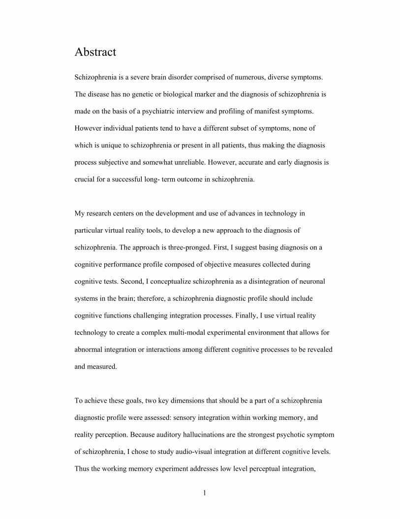
post-psychotic episodes alternating over time. 22% recover completely after one psychotic
episode (Group 1 Figure1). The remainder experience recurrent psychotic episodes with
different extents of impairment accumulating after each episode. 35% of all patients continue
to deteriorate in cognitive, social and self-caring functions after each episode (Group 4
Figure1). About half of all patients require hospitalization or extensive support environment.
2
Figure 1 Schizophrenia: Course of Illness
4 typical courses of schizophrenia. Group 1 – singly psychotic episode with full recovery; Group 2 – recurrent psychotic episodes without cognitive or functional impairment; Groups 3 – recurrent psychotic episodes with impairment after first episode only; Group 4 – recurrent psychotic episodes with deterioration of cognitive function after each episode.
Janice C. Jordan, a schizophrenic, describes her inner world in the book A drift in An
Anchorless Reality.
“During my adolescence, I thought I was just strange. I was afraid all the time. I had my own
fantasy world and spent many days lost in it. I had one particular friend. I called him the
“Controller.” He was my secret friend… I could see him and hear him, but no one else
could...
He spent a lot of time yelling at me and making me feel wicked. I didn't know how to stop
him from screaming at me and ruling my existence… I really thought that other “normal”
people had Controllers too…
I thought the world could read my mind and everything I imagined was being broadcast to
the entire world. I walked around paralyzed with fear... At one point, I would look at my
coworkers and their faces would become distorted. Their teeth looked like fangs ready to
3
devour me. Most of the time I couldn't trust myself to look at anyone for fear of being
swallowed... I knew something was wrong, and I blamed myself.”
Schizophrenia affects 1% of the world’s population, regardless of such factors as geography,
race, or socioeconomic status. There is, however, a genetic factor: 6-17% o first-degree
relatives of schizophrenia patients develop schizophrenia, whereas this figure can reach 46%
when both parents are affected and 48% in monozygotic twins 7. Another 5% of the world’s
population meet certain criteria for schizophrenia and are classified as exhibiting a schizoid
personality, schizotypal personality disorder, schizoaffective disorder, or having atypical
psychoses or a delusional disorder8.
The term schizophrenia was introduced by the psychiatrist Eugene Bleuler in the beginning
of the 20th century. It is derived from the Greek words 'schizo' (split) and 'phrene' (mind) and
refers to the lack of interaction between thought processes and perception. However,
schizophrenia was identified as a mental disease even earlier, by Emile Kraepelin in 1887.
Since then, after over a hundred years of research, many deficiencies of schizophrenia
patients have been characterized and many models proposed. However, even today the
etiology of schizophrenia remains a mystery, and the disease has no cure.
1.2 Schizophrenia as Disintegration Disorder
The leading theories today portray schizophrenia as a disturbance in integration. There is
growing evidence that supports the hypothesis that schizophrenia is associated with some
disturbance in brain connectivity:
1. Principal component analysis of PET data suggests that the normal inverse
relationship between frontal and temporal activation during verbal fluency task is

4
disturbed, showing a weak positive correlation between cerebral activation and
frontal and temporal areas in schizophrenia patients. This suggests a possible
dissociation between the two areas in these patients9. This finding was replicated
with fMRI studies10.
2. Phencyclidine (PCP), a potent inhibitor of NMDA receptors to glutamate,
induces schizophrenia-like symptoms. Glutamate neurotransmission plays an
important role in cortico-cortical interactions11.
3. Many studies show a reduced level of activation in cortical areas engaged
in a target task, as well as poor correlation or synchronization between brain areas
during different tasks. Many involve temporal-frontal activation on language
related tasks, from verbal recall and associations to mental imagery12,13.
4. Tononi and Edelman14 defined a measure of integration in the brain – a
functional cluster - as a subset of regions that are much more strongly interactive
among themselves than with the rest of the brain. When analyzing the PET data
from healthy controls and schizophrenia patients they found a significant
difference between the two groups in functional interactions within the activated
cluster, in spite of similar activation values.
As a result, a number of theories have implicated a disruption in connectivity (under
different guises) as the cause of the disease, e.g., the “cognitive dysmetria” theory proposed
by Nancy Andreasen15, the “disconnection syndrome” coined by Frith and Friston16. Peled17
suggested viewing the disturbance in connectivity as “Multiple Constraint Organization”
(MCO) breakdown. These theories will be described briefly below.

5
Disconnection Syndrome
Frith and Friston9,16 term schizophrenia a “disconnection syndrome”. They used PET and
fMRI measurements during verbal tasks to demonstrate reduced correlation between frontal
and temporal area activation. Abnormal integration of dynamics between these two regions
led them to suggest that schizophrenia may be best understood in terms of abnormal
interactions between different areas, not only at the levels of physiology and functional
anatomy, but at the level of cognitive and sensorimotor functioning.
Cognitive Dysmetria
Nancy Andreasen15 defines schizophrenia as “cognitive dysmetria”: “poor mental
coordination” in prioritizing, processing and responding to information. These features help
account for broad diverse symptoms in schizophrenia. The network responsible for
coordination is distributed not only among cortical but also sub-cortical areas (thalamus and
basal ganglia) and the cerebellum, whose role in cognition has attracted growing recognition.
Substantial anatomical connections make their way from the cortex to the cerebellum and
back to the cortex via sub-cortical nuclei. Cortical areas exchanging reciprocal connections
with the cerebellum include motor, sensory, limbic and prefrontal and parietal association
areas. Andreasen’s group showed that in normal subjects the level of cerebellar activation
correlates with prefrontal cortex activation on a number of cognitive tasks that were
unrelated to motor activity. For this reason, she suggested studying cortico-thalamic-
cerebellar-cortical circuitry in schizophrenia.
MCO breakdown
Another re-conceptualization of schizophrenia was proposed by Avi Peled17. The
organization of numerous interconnected networks in the brain can be viewed as a Multiple

6
Constraint Organization (MCO). Each connection between two units A and B defines a
constraint. The activity of unit B is constrained by the activity of unit A and by the strength
of the connection. Thus the activity of every unit is a result of multiple constraints. The
concordance of one unit’s activity with all its neighbors results in multiple constraint
satisfaction. The compliance of all units achieves MCO. This model can be readily
transferred to neural connectivity. The breakdown of MCO results in dis-connectivity or
over-connectivity that can lead to numerous symptoms of schizophrenia and a diversity of
different breakdown patterns. A detailed description is provided below.
Schizophrenia and MCO breakdown
Conceptualizing schizophrenia as Multiple Constraint Organization (MCO) breakdown, we
use the map of hierarchical and integrative organization of the brain as proposed by
Mesulam49 to define breakdown patterns. The map is shown in Figure 3. The hierarchy is
depicted as a centrifugal arrangement. The lowest hierarchical areas are on the outmost
circle, with complexity increasing toward the center. The second dimension in this map is a
division by senses, each occupying a different sector. The first hierarchical level is occupied
by primary sensory areas, which contain modality-specific topographic maps of the outside
world as perceived by the sensory organs. Next are the unimodal association areas - areas
encoding for basic features within the same modality, such as color and shape in vision.

7
41
Auditory
Visual
3b Somato-Sensory
43Gustatory
17
46
1819
21
20
22
42
5 7 8
87
Motor
Prefrontal
39
40
Posterior
Parietal37
21
Lateral
Tempo
ral
36
36
Parahip
pocam
pal
1112
1314 16
38
27 2835
232629
33
Caudal
Orbitofrontal Insula
Tempo
ral
pole
Hippocampalsystems
Primary sensory-MotorVisual (BA 17) Striat or Calcarian cortexAuditory (BA 41,42) Heschel gyrus on floor ofSylvian cisternSomatosensory (BA 3b)Anterior flank of Postcentral gyrusGustatory (BA 43) Fronto-insular junctionMotor (BA 4,6) Precentral gyrus
Unimodal association areasVisual = Peristriate connections (BA 18-19)inferotemporal regions andmiddle temporal regions (BA 21-20)Auditory = Superior (and dorsal part of)temporal cortex (BA 22)Motor = Premotor regions (BA 6,8)
Multimodal association areasPrefrontal Cortex (BA 7)Posterior Parietal Cortex (BA 39-40)Lateral Temporal Cortex (BA 37,21)Parahippocampal Gyrus (BA 35-36)
Transmodal association areasCaudal Orbito-frontal cortex (BA 11,12,13)Insula (BA 14-16)Temporal pole (BA 38)Hippocampal system (BA 27,28,35)Retrosplenial Cingulate (BA 23-26)Paraolfactory regions (BA 29-33)
Figure 3 Hierarchy of Brain Areas This map, taken from Mesulam14, conveniently represents hierarchical brain organization. Brain areas are organized on centrifugal circles from the lowest hierarchical areas, such as primary sensory areas, - on the outer circle to the highest hierarchical transmodal association areas – on the innermost circle. Each sense is represented by a sector.
Next are the multi-modal association areas, comprised of regions in prefrontal, temporal and
parietal cortices and the parahippocampal complex; these areas participate in the
transformation of perception into recognition; for example, acoustic symbols into word
meanings. The highest level of the hierarchy includes the transmodal association areas, such
as the limbic cortex. These areas constitute the highest mental functions and cover
conceptual and emotional sensation, uniting the external and internal states into a single
personal reality. This map encompasses parallel paths of information flow, intramodal as
well as multimodal areas, and bottom-up and top-down processes, thus providing a
convenient framework for the determination of the sub-types of MCO breakdown resulting
in schizophrenia symptoms.

8
For example, the left temporal cortex is responsible for retrieving word meanings from
perceived sounds, and for associating auditory perception with our knowledge about the
world. The disintegration of language perception from primary auditory areas and from
higher centers may account for auditory hallucinations. Delusions may result from MCO
breakdown in the highest association areas, by allowing states that are “wrong” or impossible
given the constraint system. Usually our perception of reality is limited or even corrected by
sensory information from the outside world and our internal knowledge about the world. The
breakdown of these constraints will create delusional concepts and percepts in spite of any
information suggesting otherwise, thus making them unshakable. This pattern may define a
“reality-distortion” type of schizophrenia, as illustrated in Figure 4b.
Disorganized schizophrenia is manifested by a mixture of conditions, when delusions or
hallucinations may be over-imposed by a weakening of associations or by unorganized
behavior. This symptomatic profile may be conceptualized as extensive breakdown both
between and within numerous areas, as in Figure 4a.
A profile involving a poverty of symptoms (both volition and emotions) is illustrated in
Figure 4c; it can be explained as a breakdown of connectivity in high association areas such
as prefrontal cortex, connecting sensation and action. Stimuli from the psychosocial
environment fail to activate responses in the patient, causing a volitional and emotional
deficit.

9
41
Auditory
Visual
3bSomato-Sensory
43Gustatory
17
46
1819
21
20
22
42
5 7 8
87
Motor
39
40
37
21
36
36
1112
13
14 16
38
272835
232629
33
41
Auditory
Visual
3bSomato-Sensory
43Gustatory
17
46
1819
21
20
22
42
5 7 8
87
Motor
39
40
37
21
36
36
1112
13
14 16
38
272835
232629
33
41
Auditory
Visual
3bSomato-Sensory
43Gustatory
17
46
1819
21
20
22
42
5 7 8
87
Motor
39
40
37
21
36
36
1112
13
14 16
38
272835
232629
33
DelusionsHllucinationsMCO
BreakdownPosteriorAssociativeareas
Prefrontal& frontalAssociativeareas
Disorganization Type I MCO-breakdown
Reality-Distortion Type II MCO-breakdown
Poverty Type IIIMCO-breakdown
a b c
Figure 4 Types of Schizophrenia as Defined by MCO-breakdown Theory A. Disorganized schizophrenia, manifesting a wide variety of symptoms, may be explained by extensive breakdown of MCO. B. Reality Distortion schizophrenia, mainly manifested in auditory hallucinations and delusions, can be explained by a breakdown of constraints in the auditory speech perception area and the highest association areas. C. Poverty schizophrenia, exhibiting negative symptoms, can be modeled as a breakdown between action and sensation networks.
1.3 Cognitive Impairment in Schizophrenia
Over a hundred years of research characterized many cognitive deficiencies of schizophrenia
patients. As a group, schizophrenia patients are impaired on almost every cognitive task
possible. In 2004 the National Institute of Mental Health established the key cognitive
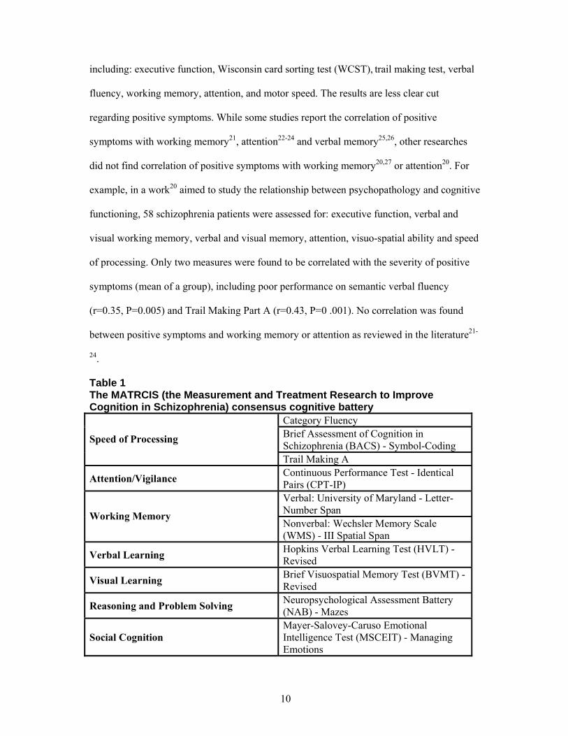
dimensions compromised in schizophrenia – the MATRICS consensus cognitive battery18,
see Table 1, where speed of processing, memory and attention are considered the most
compromised dimensions19.
Neurocognitive correlates of schizophrenia symptoms are extensively studied. It is generally
agreed that the severity of negative symptoms correlates with most cognitive deficits20,
10
including: executive function, Wisconsin card sorting test (WCST), trail making test, verbal
fluency, working memory, attention, and motor speed. The results are less clear cut
regarding positive symptoms. While some studies report the correlation of positive
symptoms with working memory21, attention22-24 and verbal memory25,26, other researches
did not find correlation of positive symptoms with working memory20,27 or attention20. For
example, in a work20 aimed to study the relationship between psychopathology and cognitive
functioning, 58 schizophrenia patients were assessed for: executive function, verbal and
visual working memory, verbal and visual memory, attention, visuo-spatial ability and speed
of processing. Only two measures were found to be correlated with the severity of positive
symptoms (mean of a group), including poor performance on semantic verbal fluency
(r=0.35, P=0.005) and Trail Making Part A (r=0.43, P=0 .001). No correlation was found
between positive symptoms and working memory or attention as reviewed in the literature21-
24.
Table 1 The MATRCIS (the Measurement and Treatment Research to Improve Cognition in Schizophrenia) consensus cognitive battery
Category Fluency Brief Assessment of Cognition in Schizophrenia (BACS) - Symbol-Coding Speed of Processing
Trail Making A
Attention/Vigilance Continuous Performance Test - Identical Pairs (CPT-IP) Verbal: University of Maryland - Letter-Number Span Working Memory Nonverbal: Wechsler Memory Scale (WMS) - III Spatial Span
Verbal Learning Hopkins Verbal Learning Test (HVLT) - Revised
Visual Learning Brief Visuospatial Memory Test (BVMT) - Revised
Reasoning and Problem Solving Neuropsychological Assessment Battery (NAB) - Mazes
Social Cognition Mayer-Salovey-Caruso Emotional Intelligence Test (MSCEIT) - Managing Emotions

11
Other studies give a mixed picture. In one study, positive symptoms were correlated with
Digit Span (r=- 0.42, p = 0.02) – a working memory measure, but not correlated with WCST,
Trail making A and B, Verbal Fluency and WAIS-R24. In a study dedicated to the
relationship between symptoms and working memory, the severity of positive symptoms was
found to be uncorrelated with performance on any of the measures27. In another study, no
clear association was found between positive symptom scores and neurocognitive deficits28.
Overall, the extensive review of verbal declarative memory by Cirillo29 reveals that positive
symptoms showed correlation with memory measures in 8 out of 29 studies. However, two
main issues complicate the comparison between different studies. First, the positive
symptoms group may contain different symptoms in different studies, with some
disagreement regarding such measures as depression, disorganization and excitement.
Second, many studies test correlation with a group of symptoms, usually summing over all
symptoms in a group, and only some look into the correlation with specific symptoms.
Auditory hallucinations are of particular interest. Brebion et al30-32 found a number of
measures correlated with auditory hallucinations, including: poor temporal context
discrimination (remembering to which of two lists a word belonged), and increased tendency
to make false recognition of words not present in the lists or misattributing the items to
another source1. An association between hallucinations and response bias (reflecting the
tendency to make false detections) was also reported in a signal detection paradigm. Bentall
and Slade33 used a task in which participants were required to detect an acoustic signal
randomly presented against a noise background. The authors then compared two groups of
schizophrenia patients, who differed in the presence or absence of auditory hallucinations, on
1 For example, they may confuse the speaker - experimenter or subject, or they may confuse the modality - was an item presented as a picture or a word.

12
the same task. The two groups were similar in their perceptual sensitivity, but differed in
their response bias. Not surprisingly, patients with hallucinations were more willing to
believe that the signal was present.
Very few studies examined the diagnostic value of the cognitive tests battery. One possible
reason is that any given patient may fall within the normal range in many tasks. The common
way to report a cognitive deficiency compares the means of the patient and control
populations, measuring the statistical significance of the difference. This procedure blurs out
individual differences, i.e. how many patients performed in the normal range, and how many
control subjects fell out of the normal range. Some reviews report that less than 40% of
schizophrenia patients are impaired34,35, while others state that a fraction of 11% up to 55%
of schizophrenia patients perform in the normal range on different tasks36-38. It is therefore
not clear whether each patient manifests some subset of cognitive impairments, or whether
some patients may preserve a completely normal cognitive function.
In an extensive study Palmer et al39 aimed to explore the prevalence of neuropsychological
(NP) normal subjects among the schizophrenia population. The authors examined 171
schizophrenia patients and 63 healthy controls using an extensive neuropsychological
battery, measuring performance on eight cognitive dimensions: verbal ability, psychomotor
skill, abstraction and cognitive flexibility, attention, learning, retention, motor skills and
sensory ability. Each dimension was measured by a number of tests. A neuropsychologist
rated functioning in each of the eight NP domains described above, using a 9-point scale
ranging from 1 (above average) to 9 (severe impairment). A participant was classified as
impaired if s/he had impaired score (≥5) on at least two dimensions. Following this
procedure, 27.5% of the schizophrenia patients and 85.7% of the controls were classified as

13
NP-normal. 11.1% of the patients and 71.4% of the controls had unimpaired ratings in all 8
dimensions. The proportion of impaired patients in each dimension varied from 9% to 67%.
In light of these disturbing results, it has been argued by Wilk et al40 that although there
exists a sub-group of patients that achieves normal scores relatively to the general
population, their score may nevertheless be lower than expected from premorbid functioning.
In other words, this sub-group might have had a higher than average premorbid score. To test
this assumption the authors tested 64 schizophrenia patients and 64 controls individually
matched by their Full-Scale IQ score. Now the patient group showed markedly different
neuropsychological profile. Specifically, these patients performed worse on memory and
speeded visual processing, but showed superior performance on verbal comprehension and
perceptual organization. These finding support the hypothesis that cognitive functioning was
impaired in these patients relatively to their premorbid level. It’s worth emphasizing that the
control group showed a consistent level of performance on all measures, while the patients
exhibited a non-uniform pattern, with some measures matching or superior to the controls
group, and some inferior.
In summary, although many cognitive deficits were established among schizophrenia
patients, the majority of them are correlated with negative symptoms, and each one is only
exhibited by a fraction of the patients. Without individual adjustments taking account of
one’s IQ and possibly other factors, cognitive tests are unable to reliably discriminate
schizophrenia patients from the remaining population. Thus there is still a need for cognitive
tests that will correlate with positive symptoms, especially with hallucinations, and for tests
which will show impairment in a greater part of the patient group.

14
1.4 The Problem of Diagnosis
Schizophrenia is expressed in numerous and diverse symptoms. Many of the positive and
negative manifestations combine to different extents throughout the course of the disease.
Each patient manifests a different sub-set of symptoms. On the other hand none of the
symptoms exhibited is unique to the disorder. Hallucinations, for example, may occur as a
result of drug or alcohol abuse. Delusions are present in manic depressive patients. Negative
symptoms are more subtle and harder to define; they may be misinterpreted as personality
traits, or may be confused with a reaction to certain life situations.
There is no biological marker to diagnose schizophrenia, and today diagnosis is made
primarily by psychiatric evaluation which relies on symptoms, medical history, interviews,
and observation. The diagnosis of all mental disorders in general, and of schizophrenia in
particular, is based on criteria specified in the Diagnostic Statistical Manual-IV (DSM). The
psychiatrist basically uses the DSM-IV as a flowchart of ‘NO’/’YES’ question to reach a
final node containing the diagnosis. Schizophrenia diagnostic criteria mainly rely on the
manifestation, and duration of symptoms and the exclusion of other medical conditions that
can result in similar symptoms. This procedure is difficult and somewhat unreliable, since
each patient’s subset of symptoms may be evaluated differently even by expert observers.
In recent years the diagnostic approach to mental disorders in general, and to schizophrenia
in particular, has come under massive attack41,42. The recently appointed National Institute of
Mental Health agenda for the upcoming DSM-V (the fifth edition of the diagnostic statistical
manual, which is to be issued in 2010) states that the DSM-defined syndromes have been
unsuccessful in forming distinct classifiable entities. More crucially, none of the DSM-
defined syndromes have been found to be related to any neurobiological phenotypic marker

15
or gene that could have etiological relevance. DSM-IV entities cannot be the equivalent of
diseases and are more likely to obscure than to elucidate research findings. Criticism has
reached a level where the Research Agenda for DSM-V calls for a paradigm shift in
psychiatric diagnosis43.
Schizophrenia is a major economic liability in the western world: in 2002 in the US alone,
overall costs linked to schizophrenia were estimated at $62.7 billion44. Even though much
progress has been made in therapeutic treatment, schizophrenia still has no cure.
Nevertheless, early and accurate diagnosis is critical for a better outcome of schizophrenia-
related deficits45.
1.5 Approach: Schizophrenia Diagnostic Profile
This dissertation describes a novel diagnostic approach that aims to combine the latest neuro-
scientific insights into schizophrenia with leading edge technology. It has three main
components: (i) describing the patient by personal cognitive profile; (ii) viewing
schizophrenia as a disruption in integration; and (iii) using virtual reality as a testing tool.
Cognitive functions rather than symptoms are used as a basis for describing a patient by a
cognitive performance profile. The success of such a cognitive profile greatly depends on its
ability to capture the main impairments of schizophrenia.
One of our routine brain functions involves the constant integration of parallel independent
information streams into a unified coherent percept of reality. Recent theoretical models
portray schizophrenia as a disruption in this global brain integration, whose breakdown
seems clinically evident in schizophrenia46,47. For example, the auditory hallucinations
typical of schizophrenia patients can occur when speech perception is not constrained by

16
primary visual and auditory inputs, enabling the individual to experience voices of non-
existent speakers48.
Therefore any schizophrenia diagnostic profile must rely on integrative tests. Further, to test
the hypothesis of disrupted integration, theoretical modeling must be backed by a powerful
measurement tool that challenges the brain in an integrative manner. Virtual Reality (VR)
technology provides the ultimate experimental environment that can reveal abnormal
integration because it is complex and multi-modal on the one hand, and fully controllable on
the other.
Personal profile
Although there is a general consensus that schizophrenia is a brain disorder, the diagnosis
and evaluation of a patient’s condition does not rely on brain functions or anatomical
regions. Diagnosis is based on the symptoms which for the most part (with the possible
exception of hallucinations and delusions) are not connected to the compromised brain
mechanism and provide no indication as to which medication would help best. We propose
to describe a patient by a performance profile, containing measurements taken during
cognitive tests. For example, a diagnostic profile of schizophrenia may contain an evaluation
of working memory, executive function, learning abilities and emotional function (see Figure
2). Though as a group schizophrenia patients are impaired on almost every cognitive task
possible, a given person can fall within the normal range on many tasks. A subject will thus
be described individually by his/her deficiencies.
Human cognitive functions are widely studied in a number of ways, including in healthy
subjects, and in those suffering from brain injuries, neurological diseases and mental

17
disorders. Describing a patient by cognitive profile will allow for a better integration of
existing knowledge in both directions: a better understanding of schizophrenia based on
other areas of research, and more complete description of cognitive function based on a
research on a schizophrenia population. This approach is not specific to schizophrenia and
may be applied to mental disorders in general. The benefits of such a profile to both the
patient and a treating psychiatrist are manifold: the measures are objective, each patient
receives a unique characterization and cognitive deficiencies are readily related to neuro-
scientific knowledge.
Figure 2 Diagnostic Profile of Schizophrenia The diagnostic profile should consist of cognitive functions impaired in schizophrenia. Examples of such functions, such as working memory and reality perception, are shown as sectors in a polar plot. A personal profile of a hypothetical subject, containing measurements collected during different cognitive tasks, is shown as a red line. The distance from the center indicates the degree of impairment, with larger distance indicating greater impairment.
To build a successful diagnostic profile a comprehensive theoretical perspective is required.
The leading theories today portray schizophrenia as a disturbance in integration. Therefore
the diagnostic profile of schizophrenia should address integrative functions.

18
Virtual reality
Immersive virtual reality is a term describing systems in which the user becomes fully
immersed in an artificial, three-dimensional world generated by a computer. The sensation of
immersion is typically achieved through the use of a head-mounted display (HMD). A
typical HMD contains two miniature display screens and an optical system that channels the
images from the screens to the eyes, thereby presenting a view of a virtual world. A motion
tracker continuously measures the position and orientation of the user's head and allows the
image-generating computer to adjust the scene representation to the current view. As a result,
the viewer can look around and walk through the surrounding virtual environment in a
similar fashion to the real world.
Virtual reality technology is especially suitable for studying schizophrenia for two main
reasons. First, schizophrenia primarily involves high-level brain functions, and therefore
some of its symptoms (such as abnormal integration) may be manifested only in an
ecologically valid environment with a strong sense of presence. Tapping multiple cognitive
and sensorimotor processes within the same testing environment makes it possible for
abnormal integration or interactions among different cognitive processes to be revealed and
measured.
Second, by replacing the traditional “boring” testing procedure with a “fun” game in a virtual
environment, the notoriously low motivation and lack of concentration exhibited by
schizophrenia patients can be better overcome. In the standard tests with buttons to press for
‘YES’/’NO’ answers, a subject can press buttons without being involved in the task. In
populations with low motivation, it is crucial to measure true inability to perform a target
task and not general impairment in motivation and concentration. To assure maximal subject

19
involvement in a task, we combined an attractive game with a test design that requires
completing a mission.
1.6 Overview of the Results
Following the Methods description, in Chapter 2, we describe the findings of the two main
experiments: the experiment studying sensory integration within working memory in Chapter
3, and the Incoherencies Detection task measuring reality perception in Chapter 4. We
further discuss how these cognitive dimensions can be combined in a schizophrenia
diagnostic profile in Section 4.2 and compare their discriminative power with standard
cognitive tests in Section 4.3. During the Working Memory experiment we found that
schizophrenia patients did not differ from the controls on the perseveration measure, as was
expected from reports in the literature on similar tasks. We investigated the reason for the
lack of perseveration in an additional experiment, Section 3.2. Finally, in Chapter 5, we
report the results on audio-visual integration in normal subjects studied using the
incoherencies detection paradigm.

20
Chapter 2
Methods
2.1 Goal
Our goal was to develop cognitive tests that could establish a partial diagnostic profile of
schizophrenia. Taking Multiple Constraint Organization breakdown as our working
hypothesis, we aim to create a disintegration profile of a subject by assessing integration at
different hierarchical levels of brain organization. The disintegration profile is complete
when the battery of psychophysical experiments covers all the integrative processes
tentatively involved in schizophrenia. Given that the most common psychotic symptom is
auditory hallucinations, we focused on testing the interaction of the auditory modality with
other areas.
We designed two experiments that reflect two dimensions of the schizophrenia diagnostic
profile: working memory and reality perception. The first test – the Working Memory
Experiment – was designed to test sensory integration within working memory - a simple
form of integration that occurs at low cognitive levels: intra-modal integration within the
visual domain such as color and shape, and multi-modal audio-visual integration. The second
experiment – the Incoherencies Detection Task - addressed audio-visual integration in
combination with higher associative areas in top-down and bottom-up processes, by means
of incoherency detection in the environment.

21
2.2 Experimental Design
An additional goal of the first experiment was to establish construct validity of Virtual
Reality in relation to standard diagnostic criteria and commonly used tools for assessing
symptoms and signs in schizophrenia. To the best of our knowledge this is the first attempt
to use VR for measuring schizophrenia deficits. Thus we sought to demonstrate that working
memory impairment, already established in schizophrenia patients50, would be manifested in
virtual reality setup similarly to what is exhibited in the standard test.
We designed a working memory task that extends the standard test and exploits the
advantages of virtual reality: (i) we use a complex game environment to activate multiple
processes instead of isolating a specific process; (ii) subjects need to remember both auditory
and visual features at the same time, whereas standard measures are either pure visual or
pure auditory memory tasks; (iii) while maintaining data in working memory, subjects must
use visual-motor skills to navigate in the maze.
In the Working Memory test the subject navigates in the virtual maze using a joystick and
head movements. To exit the maze s/he needs to remember a door-opening rule - a
combination of color, shape and sound, which changes from time to time. (The detailed
description of the experiment will follow in Section 3.1.1).
The Incoherencies Detection Task measures abnormal reality perception in schizophrenia
patients using a detection paradigm within real-world experiences. A subject is required to
detect various incoherent events inserted into a normal virtual environment. Everything is
possible: a guitar can sound like a trumpet, causing audio-visual incoherency; a passing lane
can be pink, and a house can stand on its roof, resulting in visual-visual incoherencies of

22
color and location respectively. A well-integrated brain should easily detect these
incoherencies, whereas a disturbed, incoherently acting brain should demonstrate poor
detection ability. Such failures presumably reflect disturbances of brain organization, and
could therefore provide a diagnostic tool for schizophrenia. (The full description of the task
is given in Section 4.1.1).
2.3 Virtual Reality Development
The Virtual Reality environments used in the experiments were fully in-house developed.
The Virtual Reality includes hardware elements: a Head Mounted Display, positional tracker
and joystick, and software – a 3D-grpahics computer game. The computer games were
developed in C++, using graphics packages DirectX and OpenGL. The computer game had
three main functions: generating a realistic and interactive 3D world, coordination with
navigation devices, and measuring all required parameters.
The working memory experiment had a relatively simple 3D world, containing only a few
rooms that were relocated to create continuity of the maze as the user proceeded. Figure 5A
shows an example of a room with three doors. The navigation and collection of measures
were the most challenging parts of the technical preparation of this experiment. The
navigation was implemented by two devices: the joystick that allowed movement in four
directions, and the head tracker that allowed for movement change accordingly to the user’s
head orientation. The experimental setup is shown in Figure 5B, where a subject sits in a
swivel chair and cables hang from the ceiling to enable convenient rotation in the virtual
room.

23
Figure 5 Virtual Maze Environment A. A room in the virtual maze used in the working memory task. The room contains three doors displaying a colored shape and a sound is played when a subject looks at a door. The subject needs to choose one door and open it to continue navigating in the maze. B. During the task the subject sits in the swivel chair, wearing an HMD with a positional tracker attached to it, and uses a joystick to navigate.
During navigation a subject passes through “challenge” rooms, where s/he needs to
remember a door-opening rule and make decisions, and “delay” rooms, whose purpose was
to create a delay between “challenge” rooms. We needed to keep a constant 20 second delay
throughout the task and across the subjects. This was complicated by the fact that, the speed
of navigation differed across subjects, and even for a given subject at different times. We
therefore developed a heuristic procedure to achieve an average delay of 20 seconds. After
each “delay” room the decision was reached as to whether to add another “delay” room,
based on the average speed of the subject in last five rooms and the duration of the current
delay. In addition, after a decision on last “delay” room was made, we manipulated the speed
of door opening as well as the subject’s speed to keep the delay as close to 20 seconds as
possible.
Due to the use of virtual reality we could collect non-standard measurements. For example,
by recording head position at any time we could evaluate the subject’s decision strategy –
how many doors s/he examined before making the decision, length of gaze at each door, etc.

24
The Incoherencies Detection Task contains a very complex 3D world. Obviously for an
incoherent event to pop-out the remaining virtual world has to be highly coherent and
realistic. The main technological challenge that we encountered was to build an attractive
and realistic environment that works in real-time. Unlike the Maze world that is based on
closed-space objects – the rooms, where the program has to render one or two rooms at any
given time, the Incoherencies Detection world is an open space consisting of numerous 3D
objects. The elements that contribute to realism such as good quality images, complex 3D
objects, and animation are very expensive in terms of rendering time and as a result affect
the ability to react to the user’s actions in real time. The solution to this problem included
components at all levels: from hardware - using a stronger computer and graphics card, to
software: graphic techniques for “smart” rendering, and embedding videos for motion scenes
instead of complex object animation.
The virtual world for the Incoherencies Detection Task contained a “living” neighborhood,
shopping streets and a market. To achieve maximal realism we used texture mapping of
carefully designed photos wherever possible (see Figure 6 A&B). To enhance the realism of
the virtual city, we included three dimensional moving vehicles, some with normal and some
with incoherent sounds. One example is the police car passing by, shown in Figure 6C.
However, as three dimensional object animation is expensive in rendering time, and most of
the time a naturalistic animation of 3D objects is very difficult to achieve, we used video
extensively. A video of a market vendor, embedded into a shop window, is shown in Figure
6D. Overall, the virtual city contained 22 embedded videos (see two additional examples in
Figure 6 E&F).

25
Figure 6 Incoherencies Detection Task Environment A. A living neighborhood. B. Shopping street. C. Police car going through an intersection – an example of a complex 3D animated object. D. A video scene – a market vendor, embedded in the environment. E. A woman washing the floor – a video embedded into a door frame. F. A talking parrot sits in a window, another example of a video scene.
Designing audio properties of the virtual environment was another serious challenge that we
encountered. First of all we added a constant ambient sound as a background. Creating sound
incoherencies turned out to be the most difficult part. We conducted a number of pilot trials
on students to create sound incoherency events that are perceived as such. Specifically, the

26
difficulty lies in achieving a compelling perception that a specific object emits an incoherent
sound. We found that a number of aspects help foster such a perception: (i) a moving object
is more readily linked to a sound synchronized with a source object’s movements than a
static object; (ii) localizing the sound in space along the left-right axis significantly
contributed to the desired sound-object linking, (we used a specialized sound package to
create different left and right audio streams that were delivered through two loudspeakers
located on the left and right sides of the subject); (iii) a sound should have some properties.
For example, a sound that can be easily heard on the streets, such as human voices or traffic
sounds, will not be linked to any object and will not create incoherency. On the other hand,
we noticed that an incoherency is more successful if an incoherent sound shares some
similarity with a source object.
2.4 Algorithmic Tools
In the Working Memory experiment we characterized each subject by a performance profile
consisting of 26 measurements. We developed a procedure classifying subjects into
schizophrenia patients or controls based on estimation of the distribution of performance
profiles of the healthy population. However, we had only 21 control subjects, which is much
too small a sample to evaluate the distribution. We therefore investigated different
techniques for feature selection to find a smaller subset of features that would give good
classification results. We further describe the algorithms for feature selection which were
used for data analysis in Section 3.1.5.

27
2.4.1 Mutual Information Algorithms
The information approach to feature selection is based on a calculation of the Mutual
Information between a feature (X) and a class label (Y):
))()(
),(log(),(),( ∑∑=x y yPxP
yxPyxPYXI
The Mutual Information is calculated for each feature, and the features are graded from best
to worst. A simple improvement in feature selection based on mutual information would be
to take a feature that adds maximal information to the existing feature set.
Let F be the feature set, Fi – individual feature, L – label, and G – a chosen set.
G={}.
Algorithm:
1. For each Fi in F\G calculate I, the information it adds to G
).../().../().../,(log).../,().../,(11
11...1
1kki
kikiFF
Lki FFLPFFFP
FFLFPFFLFPFFLFIk
∑ ∑=
2. Choose Fi with maximal I.
2.4.2 Margin Based Feature Selection
RELIEF
RELIEF is a popular feature selection algorithm proposed by Kira and Rendell51. In
RELIEF, each feature is assigned a weight indicating how well it separates neighboring
examples. For every data point its nearest hit – the nearest point from the same class, and its
nearest miss – a point from the opposite class are found for each feature. The feature’s
weight is updated based on the difference between the nearest hit and the nearest miss for
that feature.
Algorithm:

28
For each data point X
For each feature iF update its weight:
22 ))(())(( iiiiii xnearhitXxnearmissXWW −−−+=
Simba
The Iterative Search Margin Based Algorithm (Simba) proposed by R. Gilad-Bachrach et
al52 is one of the many enhancements that have been developed for RELIEF. Simba re-
evaluates the distances according to the updated weights and is better at eliminating
redundant features.
Algorithm:
1. initialize w = (1,…,1)
2. for t=1…T
• pick randomly an instance x from S
• calculate nearmiss(x) and nearhit(x) with respect to S\x and the weight vector
w
• for i=1…N calculate
iw
ii
w
iii w
xnearhitxxnearhitx
xnearmissxxnearmissx
)||)(||))((
||)(||))((
(21 22
−−
−−−
=Δ
• w = w + Δ
3. w <- w2/||w2||, where 22 )(:)( ii ww =
Greedy Feature Flip
Greedy Feature Flip (G-flip)52 is another algorithm proposed by the same group. It converges
to a local maximum, and thus does not require a defined size of the feature set as an input. At
each step, for every feature it evaluates a margin term with and without the feature, and

29
decides whether to keep or remove it. The algorithm stops when no change is made to the
feature set.
Algorithm:
1. initialize the set of chosen features to the empty set: F = Ø
2. for t = 1,2,…
• pick a random permutation s of {1…N}
• for I = 1 to N,
(i) evaluate )})({(1 isFee ∪= and )})({\(2 isFee =
(ii) if )}({,21 isFFee ∪=> ,
else if )}({\,12 isFFee =>
• if no change made to F then break.
Optimal Feature Selection Algorithm
The Optimal Feature Selection Algorithm (OFSA) was suggested by D.Koller et al53. It is
based on a cross-entropy measure to minimize the information lost during feature
elimination. This algorithm works in the opposite direction; specifically, it starts with a full
set of features and removes one feature at a time. The algorithm receives 2 parameters the
size of the desired subset and K – the number of features used for approximation of any
given feature Fi. Starting from the full set of features in each step one feature is eliminated
that can be predicted by the remaining K features; these K features are called the blanket.
Algorithm:
Let F=( nFF ...1 ) be a set of features, f=( nff ...1 ) set of assignment values. C1 and C2 are
classes, G – subset of features.
1. Compute the correlation coefficient of every pair of features ρij; initiate G to F.

30
)()(
),cov(
ji
jiij FSDFSD
FF=ρ
2. For each feature Fi choose K features with highest ρij to be Mi.
3. Compute δG(Fi/Mi) for each i.
∑ ======iiM
iff
MiiMiiMiiiG fMCPfFfMCPDfFfMPMF,
))|(),,|((),()|(δ
where D is cross-entropy (or KL – Kullback Leibler distance), where µ is the right
distribution and σ is its approximation, given by:
∑=x x
xxD)()(log)(),(
σμμσμ
4. Remove from feature set G - Fi with minimal δG(Fi/Mi).

31
Chapter 3
Working Memory
The first cognitive dimension that we studied was sensory integration in working memory.
The Working Memory Experiment consisted of three parts. First, we performed a pilot study
to determine which door-opening rules (i.e. combinations of features to remember) best
discriminated between the schizophrenia patients and the healthy controls. Second, we ran
the Working Memory Experiment on a large number of subjects with rules selected to study
sensory integration in working memory. We used measures collected during the task to
classify participants as schizophrenia patients or healthy controls. Third, we used the virtual
maze setup to test perseveration (a common characteristic of schizophrenia) in separate
experiment.
3.1 Experiment 1: Working Memory
3.1.1 Experimental Design
The experiment involved a computer game requiring navigation in a virtual maze with
“challenge” and “delay” rooms. Each challenge room had three doors, only one of which was
the correct choice, while each delay room had a single door. The goal of the game was to
reach the end of the maze as fast as possible, and the end was reached only after all the
correct doors had been opened.

32
Figure 7 Virtual Maze Used to Study Sensory Integration in Working Memory
A-D. “Challenge” rooms illustrating four rule types used in the experiment. Each “challenge” room has three doors with up to three features displayed: sound, color and shape. A. A door-opening rule defined by sound, with no distractor present, so the shape and color remain constant throughout a session. B. A door-opening rule defined by sound and color serves as the distractor. C. A door-opening rule defined by sound and shape, no distractor. D. The most difficult door-opening rule: a subject needs to remember shape and sound and ignore color. E. A “delay” room. To create a load on working memory a subject goes through a few “delay” rooms with one door between the “challenge” rooms. F. Positive feedback. When a subject opens a correct door, an animation of girl clapping hands appears on the door accompanied by the sound of applause, and the subject is rewarded with a cigarette or a chocolate on a score board.
Each door in a challenge room was associated with up to three distinct features—shape
(triangle, square, or circle), color (red, green, or blue), and sound (three different sounds),
see Figure 7 A-D. The sound was played when the subject examined the door. At each point

33
in time, there was a certain door-opening rule, which determined which door should be used
to exit a challenge room. For example, the rule might say that only red doors should be
opened, in which case any red door, regardless of its shape or sound, could be used. There
was always a single such door in each challenge room. The subject had to figure out the
correct rule and open only the appropriate door (with the correct combination) in each
challenge room. The rule randomly changed after 4–6 correct choices.
Table 2 Four door-opening rule types used in the final experiment
Number of
features No distractor Distractor present
1 Sound Sound + Color as distractor
2 Sound & Shape Sound & Shape+ Color as distractor
The different door-opening rules were created by manipulating two factors: the number of
features that defined the door-opening rule (one or two) and the presence or absence of a
distractor feature on the doors (a feature that was not used in the rule). In the first stage, we
created 9 experimental conditions. The four experimental conditions which discriminated
best between the schizophrenia patients and healthy control populations were chosen for the
final experiment (see Table 2 and Figure 7 A-D). The rule changed over time as indicated by
a visual cue. When the correct door was chosen, the subject received a reward (cigarette or
chocolate icon) and got encouragement (dancing figure with clapping hands), see Figure 7F.
Between challenge rooms, the subject passed through a few delay rooms, each of which had
only one door. The door in a delay room was also associated with a colored shape and sound,
and was consistently different from those used on doors in the challenge rooms (Figure 7E).

34
The delay rooms masked the target stimulus and imposed an active load on working
memory, because the subjects needed to remember the correct rule during navigation. We
manipulated the number of delay rooms to achieve a constant 20-second delay between
successive challenge rooms.
The design of the Working Memory experiment was inspired by the Wisconsin Card Sorting
Test54, in which the subject needs to sort a deck of cards into four piles. The cards display a
number of colored shapes. At any given time, the sorting needs to be done according to one
feature (out of three), which changes after 10 consecutive correct placements. In a similar
manner, each room in our maze had three doors characterized by two visual features and one
auditory feature (instead of three visual features in the Wisconsin Card Sorting Test).
While in the Wisconsin Card Sorting Test only one out of the three features displayed is
important at any moment, we controlled both the number of features that defined the door-
opening rule (one or two) and the number of features displayed (one, two, or three). There
were two additional differences: 1) how the rule was defined—in the maze, the subjects
needed to remember feature values (e.g., category values such as a red rectangle), while in
the Wisconsin Card Sorting Test the task required of the subject is to remember a category,
and 2) explanation—our subjects received detailed explanations of the task, followed by a
training session, while no explanation is provided in the standard Wisconsin Card Sorting
Test.
3.1.2 Methods
Subjects
The participants were 39 schizophrenia patients and 21 healthy comparison subjects matched
by gender (male), age, and education level. The subjects’ mean age was 32.3 years (SD=7.9),

35
and the mean number of years of education was 10.6 (SD=2.6). 10 patients and 7 controls
were exposed to 9 door-opening rule types; the remaining subjects experienced 4 door-
opening rule types, chosen in the pilot stage.
The patients were diagnosed according to DSM-IV criteria55 and were rated for symptom
severity with the Positive and Negative Syndrome Scale (PANSS)56 during an interview by a
clinical psychiatrist (Avi Peled). Schizophrenia patients with a history of neurological
disorders, co-morbidity, or drug abuse were excluded from the study. The patients were
medicated with therapeutic doses of risperidone and olanzapine. Five patients were also
taking long-acting medications (three patients were being treated with haloperidol decanoate,
and two patients with long-acting fluphenazine). In all, the patients were receiving a mean
daily dose equivalent to 414 mg of chlorpromazine.
All subjects volunteered and received payment. After a complete description of the study to
the subjects, written informed consent was obtained. The study was approved by the internal
review board of Sha’ar Menashe Mental Health Center and the Israeli Ministry of Health, in
accordance with the Helsinki Declaration.
Procedure
The experiment included a training phase intended to bring all subjects up to their best level
of performance, followed by the actual game. Training consisted of three stages. First, the
subjects learned how to find the correct door and open it (without movement); during this
stage the subjects experienced all types of door-opening rules. Second, the subjects learned
how to navigate in the maze at the desired speed. Finally, they practiced in a game-like
session, with emphasis on achieving the fewest errors (rather than speed). During training the

36
experimenter intervened when three or more consecutive errors occurred, in which case the
subject was reminded of the goals of the task, was encouraged to verbalize his strategy, and
received compliments on correct choices.
The duration of the sessions varied among subjects, since a session ended only after a fixed
number of correct doors were chosen. Upon any incorrect door choice, the subject was
presented with another challenge room with the same set of doors, shifted in position. Thus,
the session duration was positively correlated with the number of errors. In general, it took
the patients roughly twice as long to complete the training as the comparison subjects (58.6
and 28.6 minutes, respectively), while the durations of the test sessions were more similar
(31.7 and 26.4 minutes, respectively). This difference was reflected in the set of
measurements defining a subject’s profile.
A sense of reality was obtained with three-dimensional glasses, a head tracker, and a
joystick. The subjects used the joystick to navigate and to open doors. The navigation button
enabled movement in four directions: forward, backward, left, and right. A change in the
direction of movement could also be made by turning the head.
Measurements
We collected 26 measurements for each subject based on a variety of continuous physical
measures. These included error score and response time, the position and direction of gaze at
any time, and the rate of improvement over time. The 26 measurements defined the subject’s
performance profile and could be divided into three categories: working memory and
integration, navigation and strategy, and learning.
Working Memory & Integration
37
The variables reflecting working memory and integration included various error scores
measuring perseveration and the distractor and complexity effects. In calculating error scores
we differentiated 1) errors made while the subject was learning the rule (after the rule
changed), 2) errors made during use of the rule, and 3) the number of consecutive errors.
Perseveration errors occurred in all of these error categories and included any repeated
selection of a previous incorrect choice and any erroneous choice that was consistent with a
previous door-opening rule that had already changed. Perseveration was measured as the
ratio between the number of perseveration errors and the total number of errors. The
distractor effect (DE) was calculated as the error rate when the distractor was present minus
the error rate when the distractor was absent (the rows in Table 2). Similarly, the Complexity
Effect (CE) was measured as the difference in error rate between two conditions: two
features define a rule minus one feature defines a rule (the first column in Table 2).
Navigation & Strategy
The measurements of navigation and strategy included response time, navigation profile, and
strategy. The navigation profile included a measure combining navigation speed with the
number of collisions with walls and a histogram of the subject’s movements (forward,
backward, or rotation). Decision strategy was measured by the number of doors inspected in
each room and the time spent looking at each door. To assess the subject’s selection strategy,
we compared the histogram of the locations of all selected doors with the histogram of the
locations of correct doors.
Learning
The measurements of learning included the rate of improvement over time in the variables
reflecting working memory and integration, in response time, and in navigation speed.

38
All the data were normalized so that within the comparison group the values for each
variable were distributed with a mean value of 0 and a standard deviation of 1. A subject was
said to differ from the expected (normal) value for a given variable if his normalized
absolute value exceeded 2.
3.1.3 Results of the pilot study
The only difference between the pilot and the main experiment was the number of door-
opening rule types (and therefore the number of sessions) that was presented to each subject.
Otherwise the procedure, the collected measurements and data analysis were the same for all
subjects. The main results which are common to the pilot study and the main experiment will
be presented in detail in the next sections. In this section only results relevant to the door-
opening rule selection will be presented. In the pilot stage 9 door-opening rule types were
designed, see Table 3. 10 schizophrenia patients and 7 healthy controls participated in the
pilot. Each subject was exposed to all 9 rule types.
Table 3 The opening-door rule types used in the pilot experiment Number
of
features
No distractor Distractor present
Auditory (1Fa) Auditory + visual distractor (1Fa+vD)
Visual + visual distractor (1Fv+vD) 1 Visual (1Fv)
Visual + auditory distractor (1Fv+aD)
Visual (2Fv) Visual + auditory distractor (2Fv+aD) 2
Audio-visual (2Fav) Audio-visual + visual distractor (2Fav+vD)

39
Figure 8A shows the control and patient groups’ error rate for all rule types. Two rule types
were the most difficult for the patient group: the auditory rule with visual distractor
(1Fa+vD) and the audio-visual rule with visual distractor (2Fav+vD). The patients exhibited
the highest error rate for these two rule types, whereas there were no significant differences
among different rule types for the controls.
Figure 8 Error Rate when Using the Rule in the Control and Patient Groups Average error rate (when using the rule) for each of the 9 rule types in the control and patient groups. Abbreviations for rule types appear in Table 3. A. All patients (solid red line) are plotted vs. the control group (dotted blue line). B. The patients are divided into P1 – exhibiting distractor (solid red line) and complexity effects; and P2 – performing at control level (dashed green line). Already at this stage the patients could be readily divided into two sub-groups: (i) the
patients who differed considerably from control group – P1, (n=4), and (ii) the patients that
performed at control level – P2, (n=6) (Figure 8B). The P1 group, unlike the controls and P2
group, showed a significant distractor effect; specifically they made more errors in the
presence of a distractor as compared to a non-distractor condition. The number of patients

40
exhibiting the distractor effect and its magnitude are summarized in Table 4. Half of the
patients manifested the distractor effect for an auditory rule. However, for the two-feature
rules the distractor effect was the greatest.
In addition, the P1 group showed a complexity effect (made more errors in two-feature-rule
opening conditions as compared to one-feature rules) for the audio-visual rule as compared
to the auditory rule, but not for the two-feature visual rule as compared to the one-feature
visual rule (Figure 8B).
For the final experiment four door-opening rule types were used to measure the distractor
and complexity effects that discriminated best between the patient and control groups. These
four opening-door rules are summarized in Table 2.
Table 4 Distractor effect in the patient group
Vis
ual R
ule
+ V
isua
l Dis
tract
or
Vis
ual R
ule
+ A
udito
ry D
istra
ctor
Aud
itory
Rul
e +
Vis
ual D
istra
ctor
Vis
ual&
Vis
ual R
ule
+ A
udito
ry D
istra
ctor
Aud
io-V
isua
l Rul
e +
Vis
ual D
istra
ctor
Number of patients
showing DE 3 4 5 4 3
Increase in error rate
(%) in presence of
distractor
12
(SD=9)
8
(SD=6)
13
(SD=3)
21
(SD=11)
22
(SD=18)

41
3.1.4 Results of the main experiment
Highlights of the performance profile
In general, the patients differed from the comparison subjects on most of the measured
variables, while individually each patient differed on a unique subset of variables.
Specifically, the patients exhibited higher rates of errors on most measurements of working
memory and integration. The patients were significantly slower than the comparison
subjects, as expressed by poorer values on the navigation and strategy measurements.
Finally, the patients improved more than the comparison subjects, as manifested in some
learning measurements. However, no single variable differentiated the patients and the
comparison group. On any given variable, some patients differed substantially, while others
performed like the comparison subjects, resulting in high variance in all of the
measurements. Figure 9 summarizes the distributions of the comparison and patient groups
on a number of variables; the full statistics on deviation from the normal range in the patient
and control groups is given in Appendix A.
The most striking differences between the patients and comparison subjects (involving more
than half of the patients) was manifested in a higher error rate when the rule was being used
(Figure 9), more consecutive errors (Figure 9), and large head rotations (data not shown).
The patients’ higher error rate during use of the rule was maintained throughout both the
training and experimental sessions. Some patients, however, showed a marked improvement
during the training stage. In addition, a noticeable number of patients showed one or more of
the following deficits: lesser ability to ignore irrelevant information (distractor effect), higher
error rate during learning of the rule, longer response time, and poorer selection strategy
(Figure 9).
42
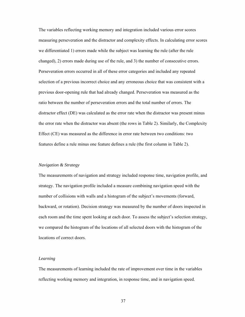
Figure 9 Normalized Scores for Selected Measurement of Schizophrenia Patients and Healthy Comparison Subjects Each circle/square represents a score of an individual subject. The scores of control (blue squares) and patient (red circles) groups were normalized so that within the control group each variable was distributed with a mean value of 0 and a standard deviation of 1. The scores of the control subjects were concentrated between –1 and 1. In contrast, the patients’ scores show a much wider distribution.
We also noted an interesting dissociation between the patients’ ability to learn a new rule and
their ability to recover from a mistake. While 23 patients showed high rates of consecutive

43
errors, only 15 patients showed high error rates when they were learning a new rule. Overall,
the patients were significantly slower than the comparison subjects, as manifested in
response time, speed, and time spent looking at doors. However, they also showed a much
greater improvement than the comparison subjects in response time and navigation speed.
Finally, there was no marked difference between the groups in decision strategy (Figure 9),
movement profile (data not shown), or perseveration (Figure 9).
To illustrate the high variance across patients, several examples of individual performance
plots are shown in Figure 10.
Figure 10 Polar Coordinates Profiling Performance of Five Schizophrenia Patients in Relation to Performance of Healthy Comparison Subjects
Each variable corresponds to a certain angle j, and the radius r reflects the subject’s measurement value on the normalized scale for that variable. Thus, a subject’s profile corresponds to a tight curve through 26 pairs of r, j coordinates. The scores were normalized as follows: 0=less than one standard deviation from the mean for the comparison subjects, 1=less than two standard deviations from the mean, 2=less than three standard deviations, 3=less than five standard deviations, 4=less than eight standard deviations, 5=more than eight standard deviations. The performance profiles of the comparison subjects concentrate by definition in the area rδ2.
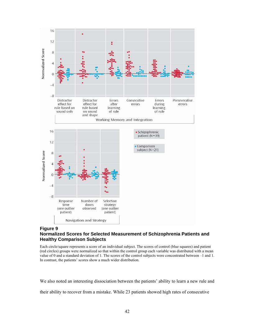
44
For instance, patient 1 performed well within the range of the comparison subjects on all but
two measurements, while patients 2, 3, and 4 deviated on a broad range of variables, each
displaying his own unique profile. Patient 2, for example, had difficulties on variables
concentrated in the upper right corner, most of which are measurements of working memory
and integration. Patient 3 showed scattered deviations in all groups of measurements, while
patient 4 differed mostly on navigation and strategy variables. Note that patient 5 performed
like the comparison subjects on all measurements.
Figure 11 Histogram of Number of Parameters Deviating More than 2SD from the Control Mean among the Control and Patient Groups
The histogram shows how many parameters the patient and control groups deviated from the control group mean. Last column shows subjects who deviated on 10 or more parameters.
Each patient deviated from the normal range on a different number of parameters (Figure
11). While the majority of the control subjects deviated on 2 or fewer parameters with only 2
subjects deviating on 4 and 6 parameters, the patient group showed a broad distribution of
parameters outside the normal range. Only 7 (out of 39) patients deviated on 1 or 2
parameters, and none of the patients performed in the normal range on all 26 parameters. On

45
the other hand, none of the patients deviated on all 26 parameters, and the greatest number of
deviating parameters -13 - was exhibited by two patients.
Distractor effect
The patient group demonstrated a somewhat lesser ability to ignore irrelevant information.
Accordingly, in the distractor conditions they exhibited higher error rates when using the
door-opening rules. The distractor effect varied greatly, with some patients exhibiting a
distractor effect only when the rule specified just one feature, some only when the rule
specified two features and some when the rule specified both one or two features. When the
distractor was absent, some patients made many errors, while others performed like the
comparison subjects. This measure—the number of errors when the distractor was absent—
reflects only the errors made after the subject had learned the rule, and therefore it mostly
reflects impaired working memory rather than inference ability.
On the basis of these two measures, i.e., the distractor effect and the number of errors when
the distractor was absent, the patients could be divided into four subgroups. Figure 12 shows
that working memory impairment and the distractor effect exhibited a double dissociation in
the schizophrenia patients. Some patients had impairment only in working memory, and
some patients had impairment only in the presence of a distractor.

46
Figure 12 Division of Schizophrenia Patients into Four Sub-groups Based on Their Working Memory and Distractor Effect Scores
The plot shows Working Memory - WM (orange bars) and Distractor Effect - DE (brown bars) scores of the control group (first column on the left) and the four sub-groups of schizophrenia patients. Schizophrenia patients can be divided into four sub-groups (from left to right on the plot): i) patients who showed both DE and WM impairment; ii) patients who exhibited DE only; iii) patients with impairment only in WM; iv) patients who performed like controls.
The WM score was defined as the minimal error rate over two door-opening rule types without a distractor: the sound rule and the sound & shape rule. The DE was taken as the maximal increase in error rate as a result of the distractor over the same two conditions: the sound rule and the sound & shape rule. Any subject differing by more than 2.5 standard deviations from the mean value of the comparison subjects was considered impaired on the relevant measure.
* Significantly different from the rate for the comparison subjects (F=65.7, df=1, 38, pδ0.001).
** Significantly different from the rate for the comparison subjects (F=43.9, df=1, 31, pδ0.001).
Complexity Effect
The rule complexity (number of features defining the rule) had no clear effect on error rate.
11 patients showed a significant difference between a one feature rule – the sound rule, and a
two feature rule – the sound & shape rule. However 5 subjects made more errors in the two-
feature rule condition and 6 subjects made more errors in the one-feature rule condition. The
control group showed no distractor or complexity effects, maintaining a constant level of
performance in all experimental conditions.

47
3.1.5 Analysis
Classification
We designed a classification routine based on the performance profiles. First, we estimated
the distribution of performance profiles with the comparison group alone. For simplicity, we
made the false assumptions that the variables were independent and that each variable had
normally distributed values. We then estimated the probability of each subject’s performance
profile under the estimated distribution. Finally, we fixed a threshold to best discriminate
between the comparison subjects and the patients in a leave-one-out paradigm. Specifically,
we fixed a probability value that best separated the comparison and patient groups, using 38
out of the 39 patients; we then checked the prediction regarding the remaining patient. The
sensitivity of this procedure was 0.85, with 33 out of 39 patients being predicted correctly.
(Canonical variate analysis correctly classified 31 patients, for a sensitivity of 0.79.
Multivariate analysis of variance indicated that the comparison and patient groups differed
significantly with p=0.00002.)
In the preceding procedure we used all 26 measurements defining the performance profiles.
However, with only 21 data points there is a high risk of over-fitting the distribution of the
comparison group. We therefore looked for the minimal subset of features that would give
the same classification accuracy. We applied the same procedure while using all subsets of
two to seven features. The minimal subset of features that achieved the same accuracy
contained four measures: distractor effect (sound and shape rule), error rate when the rule
was used during training, consecutive error rate, and response time. This set of four features
achieved same classification sensitivity as complete features set —0.85.

48
Finally, we tested the estimation procedure using a similar leave-one-out approach.
Specifically, we estimated the distribution of the comparison group based on 20 of the 21
subjects, fixed the threshold on the basis of the same 20 comparison subjects and all of the
patients, and checked the prediction regarding the missing comparison subject. As expected
from the preceding counting argument, the reduced set of four features was more robust than
the full set of 26 measurements to the leave-one-out test. The four features set achieved
100% correct classification of the comparison group (specificity, 1.00) through all leave-one-
out runs (i.e. no matter what comparison subject was left out, the procedure resulted in 100%
correct classification of the comparison group). With 26 measurements, 1 to 3 controls were
misclassified, depending on which subject was left out, overall resulting in correct
classification of only 86% (18 out of 21) of the comparison subjects. The patient group was
equally robust to the leave-one-out test for both full and four features sets, resulting in the
same number of misclassified patients through all leave-one-out runs.
Feature Selection
By testing all subsets of features of sizes 2-7 we found a set that achieved the same accuracy
as 26 features and was robust to the leave-one-out test. An additional important parameter to
consider is which subjects were misclassified; in this case we preferred to miss a patient than
falsely identify a control as a patient, i.e. we do not want to improve sensitivity at the
expense of specificity. Other subsets of 6-7 features gave us the same number of
misclassified subjects - 6, but included misclassified controls. Can a larger size subset give
us better accuracy, restore the specificity and maintain robustness to the leave-one-out test?
To test all subsets of features 2-26 was too time -consuming. We therefore investigated a
number of algorithms for feature selection (described in Section 2.3).

49
For each algorithm we chose the 10 best features, see Appendix C, and tested all subsets of
sizes 4-10 in our classification procedure as described in the previous section. We further
reported the best result of each algorithm in terms of classification accuracy and robustness
to the leave-one-out test. The best result still remained the four features set found in the
previous section that predicted correctly all the controls and 85% of the patients (6 patients
misclassified) and maintained the same result through all leave-one-out runs.
We started with the most straightforward approach: to grade the features by mutual
information of each feature and a class label. Though some of the subsets of features with the
highest mutual information predicted overall more subjects correctly, they all falsely
reported 2 controls as patients. The best result with 4 misclassified subjects was achieved by
a set of 8 features. Improving the feature grading by choosing a feature that added maximal
information to a chosen set at each step resulted in the best subset of 4 features with 7
(instead of 6) misclassified patients and all controls predicted correctly.
We further tried margin- based feature selection algorithms. We started with one of the most
simple and popular algorithm – RELIEF. In RELIEF the feature score depends on how well
it separates neighboring examples. The best subset was of size 10 and misclassified 8-9
subjects, among them 0-1 controls. The drawback of this algorithm is that predictive but
correlated features are given high weight; in our case it twice chose pairs of highly correlated
features: the error rate when the rule was used and the error rate when learning the rule
during training and experimental sessions, see Appendix C for the chosen feature subsets.
We next used Simba – the Iterative Search Margin Based Algorithm, that should overcome
the problem of redundant feature selection. The Simba indeed did not choose trivially

50
redundant features and improved prediction relative to RELIEF: the best set consisted of 10
features and misclassified 7 subjects, which is one subject more than our best four features
set.
The Optimal Feature Selection Algorithm (OFSA) finds the optimal subset of features of
given size. The OFSA starts with full set of features and eliminates one feature that will
cause minimal loss of information. The optimal subsets of 4-10 features chosen by the OFSA
are summarized in Appendix D. The best result of the OFSA was 8 misclassified patients (9
features) or 7 misclassified subjects, among them 2 controls (10 features).
The drawback of all the above algorithms is that they do not choose the optimal sub-set of
features but either grade the features from worst to best or find an optimal sub-set of a given
size. The Greedy Feature Flip (G-flip) converges to a local maximum, and thus does not
require a defined size of features set as an input. The G-Flip belongs to the family of margin
based algorithms: at each step, for every feature it evaluates a margin term with and without
the feature, and decides whether to keep or remove it. The algorithm stops when no change is
made to the feature set. We tested two versions of G-flip based on linear and sigmoid
evaluation functions. The linear G-flip chose 8 feature, see Appendix C. This set was not
very robust to the leave-one-out test and ranged from 5-11 missed patients and 1-3 controls
falsely identified as patients. The sigmoid G-flip converged to 6 feature set. It misclassified
10 patients and up to 2 controls.
Correlations with symptoms
To study the correlation between our measurements and the subjects’ PANSS scores,

51
we assigned “absent” to the comparison subjects on all symptoms, normalized the PANSS
scores and normalized measurement scores to a 0–5 range, see Table 5.
Table 5 The normalization that was applied to the performance profile normalized scores and PANSS values
Performance Profile PANSS
Score Normalized score Score Normalized score
s<1 0 1-2 Absent or Minimal 0
1 ≤ s < 2 1 3 Mild 1
2 ≤ s < 3 2 4 Moderate 2
3 ≤ s < 5 3 5 Severe 3
5 ≤ s < 8 4 6 Severe 4
s > 8 5 7 Extreme 5
The correlation coefficients of all parameters of the performance profile with 7 positive and
7 negative symptoms are given in Appendix B. The analysis revealed a number of significant
correlations (Spearman r≥0.4, t≥3.32, df=58, p<0.01, see Table 6): 1) the error rate during
use of the rule (after the rule was learned) was significantly correlated with five positive and
four negative symptoms, 2) the consecutive error rate was correlated with six negative
symptoms, 3) the distractor effect for the sound-based door-opening rule was correlated with
six positive symptoms, while the distractor effect for the sound-and-shape rule was
correlated with only one positive symptom (conceptual disorganization), 4) longer response
time was correlated with six negative symptoms, and 5) poor selection strategy was
correlated with six positive symptoms. None of the variables showed any significant
correlation with age. When using canonical correlation analysis to measure correlations

52
between mixtures of variables, we found two significant correlations including the same
group of highly correlated measures and symptoms.
Table 6 Summary of significant correlations for selected parameters All correlations reported here have Spearman r≥ 0.4, t ≥ , p<0.01. The four parameters used for classification are shown in bold. Positive symptoms include delusions, conceptual disorganization, hallucinatory behavior, excitement, grandiosity, suspiciousness and hostility. Negative symptoms include blunt affect, emotional withdrawal, poor rapport, passive, difficulty in abstract thinking, lack of spontaneous conversation and stereotyped thinking.
Number of symptoms in correlation with a parameter Parameter
Positive (7) Negative (7) General (16)
Distractor effect, sound & shape rule
1 - -
Errors when using the rule 5
4
6
Consecutive errors 2
6
7
Response time 1
6
10
Distractor effect, sound rule 6 - 3
Complexity effect - - 2
Errors when learning the rule - - 1
Poor selection strategy 6
1
3
Over-rotation 4 7 9
3.1.6 Discussion
We used virtual reality technology to design a complex environment for the study of
schizophrenia. The technology made it possible to collect multiple measurements during a
complex behavior, including multimodal interactions that place a high load on working

53
memory. In addition, the technology allowed us to conduct the experiment as a game and
engage the patients in the task, which improved the subjects’ concentration and motivation.
The most important finding from this experiment is that schizophrenia patients can be
reliably separated from comparison subjects on the basis of the profile of their performance
in the virtual maze. The classification procedure succeeded in predicting correctly 33 (85%)
out of 39 patients and all of the comparison subjects, by using performance profiles
consisting of four measures: distractor effect, error rate during use of the rule during training,
consecutive error rate, and response time. A closer look at the performance profiles of the
misclassified patients revealed that they fell in the normal range on almost all the variables
studied.
This experiment concentrated on working memory, which is not the only known deficiency
of schizophrenia patients. Thus, the schizophrenia diagnostic profile should evaluate a wider
spectrum of cognitive functions. Feature selection analysis revealed that the majority of sub-
sets are unstable to the leave-one-out test. This resulted from the small size of the data set
relative to the number of parameters in the performance profile. Other powerful
classification techniques that are based on training and test sets could not be applied for the
same reason. The experiment should be run on a larger number of controls, to improve
estimation of the control population distribution, and especially that of the patients, a group
that presents great variability. Furthermore, the routine should be evaluated with additional
comparison groups consisting of patients with different mental disorders.

54
On the positive side, some of the measured variables showed significant correlations with
standard measures of schizophrenia (based on personal interviews), leading us to hope that
similar tests may be able to replace subjective interviews in future diagnosis of the disease.
Finding functional sub-divisions within the patient group is another goal of our research. We
divided the patients into 4 sub-groups based on the working memory measure and distractor
effect; however this division did not result in clear separation on other parameters.
Schizophrenia probably involves multiple sub-types. In order to characterize the sub-types a
larger number of patients should be tested.
Two additional findings are worth noting: (i) decreased ability to ignore irrelevant
information, measured by the distractor effect; and (ii) a complexity effect, measuring a
simple form of integration of two features from different modalities: sound and shape.
Schizophrenia patients are known to possess an increased tendency to react to irrelevant
stimuli. About 40% of the patients manifested a distractor effect in at least one condition
(one or two-feature rule).
Rule complexity had little effect on patients’ performance and no effect on the controls. In
general it isn’t known what complexity effect is expected. On the one hand, a sound feature
is more difficult to remember and distinguish than a visual feature. It is likely that a visual
feature in sound & shape rule makes it easier to remember and recognize the correct door,
thus turning sound & shape into an easier condition. On the other hand, if a constraining
factor is load on working memory, then remembering two features could be a more difficult
condition. There is a tradeoff between a single feature difficulty and load on working

55
memory. We did not observe the complexity effect in the healthy population, probably
because of the simplicity of the task.
Knowing that schizophrenia involves an integration disturbance, we could expect to find a
distractor effect in a larger number of patients or that sound & shape rule would be more
difficult for the patients. However, the disorder is complex and it appears that the integration
problems are manifested in higher functions rather than on the perceptual level.
3.2 Experiment 2: Perseveration
Perseveration is a common indicator of schizophrenia57. In the working memory experiment
the patient group did not differ from the control group on the perseveration measure.
However, our approach to measuring perseveration differed in two ways from the classical
procedure such as the one used in the Wisconsin Card Sorting Test. First, we measured
perseveration by a ratio—the number of perseverative errors divided by the total number of
errors. This is because when the total number of errors is high, the number of perseverative
errors is expected to be high as well, irrespective of the source of error. Indeed, the numbers
of total and perseverative errors showed a high correlation (rs=0.87). Second, in our
experiment the subjects received a detailed explanation of the task, in addition to extensive
training. This difference might explain the discrepancy between our results and those in the
relevant literature. To test this hypothesis, we designed an additional experiment, described
below.

56
3.2.1 Design
This experiment was designed to investigate the underlying reason for the absence of
perseveration in the working memory experiment and, specifically, the relation between task
understanding and perseveration. We tried to replicate the standard Wisconsin Card Sorting
Test as closely as possible in our virtual maze. The experiment was conducted in the same
virtual maze used in the main experiment, with the rule defined by just one feature, color,
and without a distractor. The goal of the game was to find the correct door by which to exit
each room. Two experimental conditions were compared: 1) when the subjects were not told
what defines a correct door and 2) when the subjects were told that the correct door is
defined by color and that the correct color may change. If perseveration indeed results from
the subject’s inability to adapt his behavior to change, the number of perseverative errors
should be the same in both conditions.
3.2.2 Method
The participants in this experiment were 21 schizophrenia patients and 19 comparison
subjects. They are described in the methods section for the main experiment (most of them
later participated in the working memory experiment). The subjects received some initial
navigation training. The game ended after the opening of 50 doors. The correct color
changed after 10 consecutive correct choices.
We collected the same standard measurements as used in the Wisconsin Card Sorting Test,
among them the number of colors completed, maintaining set (the number of consecutive
correct choices), perseveration to previous color (the number of times that the previous
correct color is chosen after the rule changes), perseveration to previous incorrect color (the
number of times that some incorrect choice is repeated), the number of steps to learn the first

57
color, the number of steps to find the correct color after the first change, and the average
number of steps to learn a new color after a change. In addition, the navigation and strategy
variables used in the working memory experiment were measured. The data were analyzed
by two-way analysis of variance for the effect of two factors: explanation and group type
(patient or comparison).
3.2.3 Results
In the patient group, the scores on a number of variables were affected by explanation
(Figure 13). On the other hand, the comparison group performed equally well in the two
experimental conditions on all of the measurements.
In addition, the patients differed from the comparison subjects on navigation and strategy
variables regardless of the experimental condition, in a way similar to that in the working
memory experiment. Only patients who did not receive the explanation exhibited high
perseveration rates of both kinds (Figure 13). The explanation effect in the patient group was
also manifested in 1) the number of colors learned, 2) maintaining set (number of
consecutive correct choices), 3) the number of steps to learn a new door-opening rule after
the initial change, and 4) the average number of steps to learn a new rule after a change. The
first three effects are shown in Figure 13; significant effects are denoted by asterisk. In
addition, the patient group had a longer response time (Figure 13) and slower navigation
speed, made more collisions, and inspected more doors in the challenge rooms before
making a decision.

58
Figure 13 Effect of Explanation on Performance of Schizophrenia Patients and Control Subjects
*1Significant difference between conditions (F=18.75, df=1, 19, p=0.0004). *2Significant difference between conditions (F=6.40, df=1, 17, p=0.03). *3Significant difference between conditions (F=20.89, df=1, 19, p=0.0002). *4Significant difference between conditions (F=17.77, df=1, 38, p=0.0001).
3.2.4 Discussion
Our results indicate the need to clarify the notion of perseveration. In the working memory
experiment, the patients did not differ from the comparison group on the perseveration

59
measure. In the perseveration experiment, we found high numbers of perseveration errors
only when the patients did not receive an explanation of the task. This deficiency was
correlated with other measures related to task understanding. This finding implies that
perseveration as measured in the standard Wisconsin Card Sorting Test may indicate a
deficiency in problem solving, rather than the patients’ inability to adjust to changes (as is
usually understood). It is consistent with other reports that schizophrenia patients can
dramatically improve after training on different tasks58,59.

60
Chapter 4
Reality Perception
In this experiment we investigate audio-visual and visual-visual integration tapping higher
cognitive processes using an Incoherencies Detection Task (IDT), Section 4.1. In Section 4.2
we discuss how working memory and reality perception can be combined in a schizophrenia
diagnostic profile.
4.1 Reality Perception in Schizophrenia Patients
4.1.1 Experimental Design
This experiment was designed to measure abnormal reality perception in schizophrenia
patients using a detection paradigm that incorporates real-world experiences. Subjects were
required to detect various incoherent events inserted into a normal virtual environment.
There were three categories of incoherent events: (i) an incoherent sound, for example, an
ambulance with a horn playing an ice-cream truck melody, resulting in an audio-visual
incoherency; (ii) an incoherent color, such as blue potatoes, or (iii) an incoherent location,
such as a giraffe in a store, The latter two categories are examples of visual-visual
incoherency (see Figure 14).
Subjects sat comfortably in a reclining chair, wearing a Head Mounted Display (HMD)
containing the audio and visual devices and a position tracker. The HMD delivered the
virtual reality and created a vivid sense of orientation and presence. Subjects navigated along
a predetermined path through a residential neighborhood, shopping centers and a street

61
market (Figure 14). Aside from the incoherencies which were deliberately planted, the
virtual environment was designed to resemble the real world as closely as possible.
Figure 14 Examples from the Virtual World Used in the Incoherencies Detection Task Three categories of incoherencies are shown: A. incoherent color; B. incoherent location; C. incoherent sound: a guitar making trumpet sounds, and an ambulance sounding like an ice-cream truck.
Whenever the path traversed an incoherent event, progress was halted and a one-minute
timer appeared, during which the subject had to detect the incoherency. The response
included marking the whereabouts of the incoherent event by a mouse click, and an
accompanying verbal explanation which was recorded. A response was only scored as
correct if the subject provided an acceptable explanation. If the explanation wasn’t clear the

62
experimenter could pose clarification questions. We gave no examples before the test as
guidelines, and no feedback indicating correct or incorrect detection. (A demonstration
movie of the virtual world can be found at
http://www.cs.huji.ac.il/~daphna/movies/vr_inconsistencies/Demo_best.swf).
The three categories of incoherent events are depicted in the following figures: sound (Figure
14C), color (Figure 14A) and location (Figure 14B). The virtual world contained 50
incoherencies: 16 involving color, 18 concerning location and 16 related to sound
4.1.2 Method
Subjects
43 schizophrenia patients were recruited for the study - 23 in-patients from the inpatient
population of the Shaa’r Menashe Mental Health Center, and 20 out-patients from the
“Hesed veEmuna” hostel in Jerusalem. 29 healthy controls were matched by age, education
level and gender to the patient group. Mean age was 32.6 (SD=8.5), with an average of 11.1
(SD=1.8) years of schooling; 19% were females.
All patients had a psychiatric interview with a senior psychiatrist (Avi Peled), which adhered
to the guidelines of the Structured Clinical Interview for DSM-IV Axis I Disorders32, and the
diagnosis of schizophrenia was established according to DSM-IV-TR criteria. The severity
of schizophrenia was assessed by the Positive and Negative Syndromes Scale (PANSS)33.
Exclusion criteria included history of neurological disorders and substance abuse in the
previous 3 months. The patients were medicated.
The study was approved by the Sha'ar Menashe Mental Health Center Review Board, and
informed consent was obtained from all participants after the nature of the study was fully

63
explained to them. All subjects volunteered and received payment. They were tested for
color blindness by a color naming procedure and anamnesis.
Incoherencies Set
The pilot study was performed on student volunteers to choose incoherencies that were
recognized by 90% of the subjects. The complete list of incoherencies used in the experiment
is given in Table 7. To balance incoherent sound events we included 12 normal sound events
that were inserted into scenes with incoherent color or location (as noted in ‘Remarks’
column in Table 7). All subjects navigated along the same path in the virtual world and saw
the incoherent events in the same order.
Table 7 List of incoherencies used in the experiment The incoherencies are listed in their order of presentation. For each incoherency an object and its incoherent property is listed. For the sound incoherencies a categorical relation between a source object and a sound is given in ‘Remarks’ column. Normal sounds are also indicated in the ‘Remarks’ column.
Incoherent Object Incoherent Property
Category Remarks
1 Roof Under the house Location
2 Dog Cow Sound Same Category
3 Palm Purple Color
4 Passing Lane Purple Color Police car – normal sound
5 Chair On the roof Location
6 Street Sign Upside down Location Cat – normal sound
7 Cloud Red Color
8 Lawnmower? Fax Sound Same Category
9 Baby tapping on plastic can Cymbals Sound Same Category
10 Hydrant In the middle of the road
Location Car – normal sound

64
11 Airplane Bombing Sound Same Object
12 Plant Blue Color Dog – normal sound
13 Floor washing Toilet flushing Sound Same Object
14 Traffic Light Sidewalk Location
15 Ball Bells Sound Different Category
16 Israeli Flag Red Color Wind Chimes – normal sound
17 Parrot Chicken Sound Same Category
18 Cat Dog Sound Same Category
19 Cows Bus station Location
20 Guitar Trumpet Sound Same Category
21 Cannon Clothes store Location
22 Ambulance Ice-cream truck Sound Same Category + traffic light – normal sound
23 Face Green Color
24 Dog Office Location
25 Closing Door Breaking glass Sound Same Category
26 W.C. Book store Location
27 Bus Elephant Sound Different Category
26 Traffic Light Purple and red Color Traffic light - normal sound
29 Coca-cola vending machine Blue Color Rotating door –normal sound
30 Cabbage Blue Color Drumming – normal sound
31 Penguins Store counter Location
32 Potatoes Blue Color Merchant – normal sound
33 Eggs Pink Color
34 Tomatoes Blue Color
35 Bird Nest Merchant’s head Location

65
36 Merchant Lion Sound Different Category
37 Apples Purple Color
38 Child’s face Watermelons Location Merchant – normal sound
39 Bananas Purple Color
40 Soldier’s uniform Purple Color Tower clock – normal sound
41 Giraffe Art Gallery Location
42 Orthodox Jew’s coat Multicolored Color (instead of black)
43 Pig Store counter Location
44 Car Train Sound Same Category
45 Construction Truck Gun fire Sound Different Category
46 Shop Sign Reversed left-right
Location
47 Eye (advertisement stand) Mouse Location
48 Adults Laughing Baby Sound Same Object
49 Koala Baby Pouch Location
50 Lion’s head (advertisement stand)
Woman’s body Location
Data Analysis
Three incoherencies were excluded from the final analysis: two (blue cabbage and soldiers in
purple shirts (see Figure 15, incoherencies 30 and 40 respectively), due to the high miss rate
(≥25%) among the control subjects: and one due to repeated reports of its being confusing –
a woman holding a koala in a frontal baby pouch. This resulted in 14 incoherencies for color,
17 - location, 16 – sound, for a total of 47.
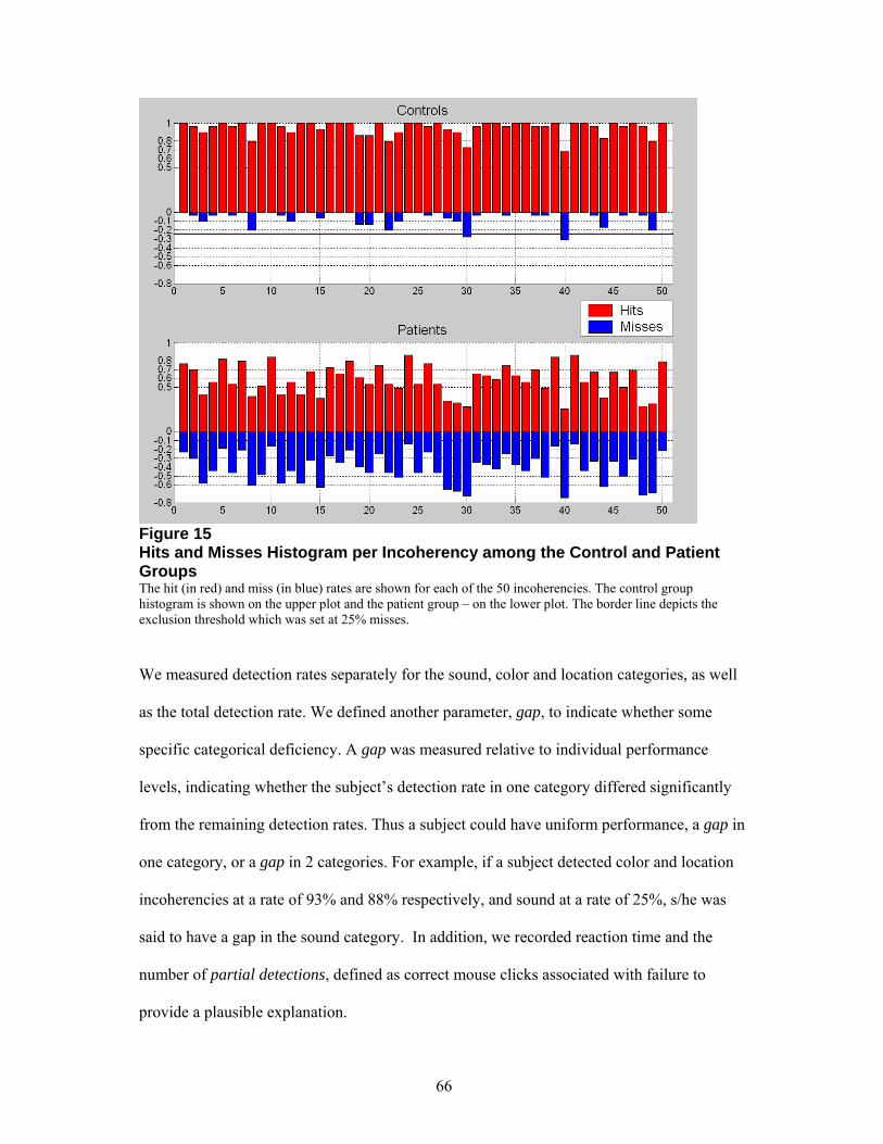
66
Figure 15 Hits and Misses Histogram per Incoherency among the Control and Patient Groups The hit (in red) and miss (in blue) rates are shown for each of the 50 incoherencies. The control group histogram is shown on the upper plot and the patient group – on the lower plot. The border line depicts the exclusion threshold which was set at 25% misses.
We measured detection rates separately for the sound, color and location categories, as well
as the total detection rate. We defined another parameter, gap, to indicate whether some
specific categorical deficiency. A gap was measured relative to individual performance
levels, indicating whether the subject’s detection rate in one category differed significantly
from the remaining detection rates. Thus a subject could have uniform performance, a gap in
one category, or a gap in 2 categories. For example, if a subject detected color and location
incoherencies at a rate of 93% and 88% respectively, and sound at a rate of 25%, s/he was
said to have a gap in the sound category. In addition, we recorded reaction time and the
number of partial detections, defined as correct mouse clicks associated with failure to
provide a plausible explanation.
67
The normal range for a given parameter was defined as the mean of the control group ±2.5
SD, the range that included roughly 99% of the normal population.
4.1.3 Results
We analyzed the results in a number of ways. First, we analyzed the detection rates, which
showed a very clear and significant difference between the control group (with close to
perfect performance) and the patient group (with typically poor performance). Second, we
defined and analyzed the gap phenomenon, which showed that patients had much larger
variability in their responses as compared to the control group. Third, we analyzed verbal
responses and found that the patient group had difficulty in explaining an incoherency even
when the object was identified correctly. Fourth, we measured the correlations between the
patients’ PANSS scores and the measurements obtained in our experiments. Notably, there
was a strong correlation between increased hallucinations and poor detection rate in our
experiments. Finally, we analyzed the various types of incoherent events, categorizing them
and ranking them according to their discriminability.
Detection Rates
The control group easily identified most of incoherencies; the hit and miss rates for all
incoherencies are shown in Figure 15. Only two incoherencies were detected by fewer than
75% of the controls, and were therefore excluded from the final analysis. About 50% of the
incoherencies were detected by all control subjects, while none of the incoherencies was
detected by all the patients. About a third of the incoherencies were detected by less than
50% of the patients.

68
Figure 16 Histograms of Hit Rates among the Control (on the left) and Patient (on the right) Groups Horizontal axis represents detection rates, and vertical axis shows the number of subjects with this score. The different plots show total hit rate, as well as hit rate in each category: color, location and sound. The red (grey in B&W) bars show subjects who performed in the normal range (defined as the mean value of the controls group ±2.5 SD). The blue (black in B&W) bars show subjects who performed below the normal range.
The histogram of detection rates in the control and patient groups is shown in Figure 16. The
control subjects detected incoherencies very well, with an accuracy level of 96% on average
(SD=4) (left panel). In general, the patient group (right panel) differed significantly from the
controls. Normal detection rates are shown in red for each category, whereas blue bars
indicate the number of subjects who performed below normal. For example, the normal
range for total detection rates is 87-100%. The upper plot shows that all but one of the
control subjects performed in this range. Among the patients only 6 subjects (red bars)
performed in the normal range, whereas 37 subjects (blue bars) had lower detection rates.

69
The patient group exhibited the most difficulty in the sound category: 30 patients performed
below the normal range, and 19 had detection rates below 50%, compared to the location
category, where only 10 patients detected fewer than 50% of the incoherencies. These and
other statistics on the control and patient groups are summarized in Table 8.
Table 8 Detection rates and other statistics for the control and patient groups Controls Patients
Mean(std) detection
rate in %
Number, below
control mean +2.5
std
Number, below
50% detection
Total 96 (4) 37 (86%) 11 (26%)
Sound 94 (7) 30 (70%) 19 (44%)
Color 95 (7) 28 (65%) 15 (35%)
Location 98 (4) 25 (58%) 10 (23%)
Gap phenomenon and various divisions of the patient group
The control group showed similar detection rates in all three categories (Figure
17A). The patient group, on the other hand, could be divided into two major sub-groups
based on the similarity in detection rates. (1) The uniform group – patients whose detection
rates in all three categories were similar. (2) Gap – the group of patients having specific
difficulty in one or two categories. A patient was defined

70
Figure 17 Individual Performance Plots of the Control Subjects and Schizophrenia Patients The horizontal axis represents three detection categories: sound, color and location, while the vertical axis shows the detection rate of the subjects in a given category. A. The control subjects exhibit similar detection rates throughout the different categories. The patients are divided into two groups: subjects with uniform performance (B, C and D) and subjects having a gap in either one (E) or two categories (F). The patients with uniform performance can be further divided by level of performance to: B. normal range; C. fair performers (below normal range but above 50%), and D. poor performers (below 50%); E. The patients with a gap in the sound category; F. The patients with a gap in the sound and color categories.
as having a specific impairment in one category – or gap – if this category score was
significantly below his/her best category (a significant difference is a difference exceeding
the mean±2.5SD of the control group). The uniform group could be further divided into: i)
uniform normal: patients performing at normal levels (N=5 subjects, Figure 17B); ii) uniform
fair: patients with fair detection rates (50-87%) but below the normal range (N=10 subjects,
Figure 17C); and finally iii) uniform poor: patients with poor uniform performance below
50% (N=8 subjects, Figure 17D). Almost half of the patients (the gap group) had specific
difficultly in one or two categories. 16 patients (37%) had a specific difficulty in detecting

71
audio-visual incoherencies: 7 patients had difficulty in the sound category only (Figure 17E),
7 patients had difficulty in the sound and color categories as compared to the location
category (Figure 17F) and 2 patients had difficulty in the sound and location categories. Only
4 patients had other specific difficulties. The number of patients belonging to each of the
above groups is summarized in Table 9.
Table 9 Sub-groups of patients defined by performance Number of
patients % of patients
Normal 5 11.6%
Fair 10 23%
Poor 8 18.6% Uniform
Total 23 53.5%
in Sound category only 7 16.3%
in one other category 3 7%
in 2 categories: Sound & Color/Location
7 / 2 20.9%
in 2 categories: Color and Location
1 2.3%
Gap
Total 20 46.5%
Verbal Response Analysis
Detection was only scored as correct if the subject provided a plausible explanation. Each
incoherency could be explained by two arguments: an object and an incoherent property. For
example, for a red cloud, the explanation had to contain an object word – cloud or sky and a
word referring to a color: considered acceptable were such phrases as “wrong color”, “red”,
or “should be blue/grey/white”. Thus, each incoherency was defined by two “anchor” words

72
that had to be present in the explanation. Based on this definition all responses were rated for
correctness by the experimenter.
However, as the experimenter was aware of subject’s assignment to the control or patient
groups, her ratings could be biased. Therefore, a number of external observers, blind to the
purpose of the experiment and the assignment to patient vs. control group, analyzed the
(recorded) verbal response associated with each incoherency detection. They ranked the
answer as correct or incorrect, and provided some additional ranking as explained below.
The external observers rated the responses of 62 out of 72 subjects, 4 subjects could not be
rated because of poor recording quality and 6 subjects who spoke Russian.
The compatibility of the experimenter and external observers’ ratings is shown in Table 10.
For the entire control group the experimenter’s and the external observer’s rating differed 13
times: 10 times the experimenter accepted an explanation and the external observer did not,
and 3 times vice versa; overall resulting in 99% compatibility in judgments of the correctness
of explanation. In the patient group the compatibility was 92%, which reached 94.3% when
discarding disagreements that did not affect the final detection scores (second column in
Table 10). For both groups the experimenter tended to accept explanations as correct more
readily than the external observers. This effect had little impact on the control group where
there was 99% compatibility.
Because in the patient group the experimenter scored more the patients more favorably, the
rating differences were not detrimental to the results in any way. Taking into account that
compatibility between the ratings was very high, and that the experimenter’s rating is more
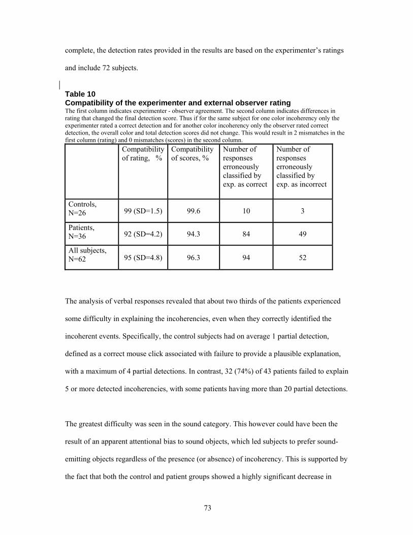
73
complete, the detection rates provided in the results are based on the experimenter’s ratings
and include 72 subjects.
Table 10 Compatibility of the experimenter and external observer rating The first column indicates experimenter - observer agreement. The second column indicates differences in rating that changed the final detection score. Thus if for the same subject for one color incoherency only the experimenter rated a correct detection and for another color incoherency only the observer rated correct detection, the overall color and total detection scores did not change. This would result in 2 mismatches in the first column (rating) and 0 mismatches (scores) in the second column. Compatibility
of rating, % Compatibility of scores, %
Number of responses erroneously classified by exp. as correct
Number of responses erroneously classified by exp. as incorrect
Controls, N=26 99 (SD=1.5) 99.6 10 3
Patients, N=36 92 (SD=4.2) 94.3 84 49
All subjects, N=62 95 (SD=4.8) 96.3 94 52
The analysis of verbal responses revealed that about two thirds of the patients experienced
some difficulty in explaining the incoherencies, even when they correctly identified the
incoherent events. Specifically, the control subjects had on average 1 partial detection,
defined as a correct mouse click associated with failure to provide a plausible explanation,
with a maximum of 4 partial detections. In contrast, 32 (74%) of 43 patients failed to explain
5 or more detected incoherencies, with some patients having more than 20 partial detections.
The greatest difficulty was seen in the sound category. This however could have been the
result of an apparent attentional bias to sound objects, which led subjects to prefer sound-
emitting objects regardless of the presence (or absence) of incoherency. This is supported by
the fact that both the control and patient groups showed a highly significant decrease in

74
detection rate of color and location incoherencies when a normal sound event was present in
the scene. The control group exhibited a 6% decrease (T-test t= 3.0430 , df=28, p=0.005), and
the patient group – an 18% decrease (T-test t =5.5425, df=42, p= 1.8024 e-006).
To test the assumption of bias to sound objects we verified which object was reported as
incoherent in the case of wrong detection of color and location incoherencies accompanied
by a normal sound event. Table 11 shows, for every incoherency, the number of times that a
normal sound object was reported as incoherent for the patient and control groups. In
addition it lists all other objects that were reported as incoherent and the number of times
each object was mentioned. To test the bias to sound objects we compared the average
frequency of sound object reports with all other object reports.
The control group did not show any clear bias to sound objects, with an average frequency of
1 for sound objects reports and 1.7 for other objects. However the control group was smaller
and had many fewer misses, approximately 10%. On the other hand, the patient group
mentioned a sound object as incoherent on average 5.8 times (SD=4.7), while other objects
were mentioned with a frequency of 1.9 (SD=1.6), the most frequent non-sound object was
reported on average 3.8 times. The patients’ bias to sound objects was highly significant
(df=60, F=23.47, p=9.3e-6).

75
Table 11 Objects identified as incoherent in presence of normal sound event The numbers show how many times an object was reported as incoherent. The objects that were indeed incoherent and were mentioned as such but no proper explanation was provided are marked in italics. Incoherency – normal sound
Reports of sound object
Reports of other objects
Controls, N=26
Patients, N=34
Controls Patients
Pink passing lane – police car
1 8 - 2 – passing lane 1 – fruits
Up-side street sign – cat
1 15 - 1 – window 1 – traffic light 1 – street
Hydrant – car 0 0 - 2 – barrier 1 – road, 1 – door 1 – tr. Light, 1 – doll 1 – passing lane
Blue plant – dog 2 11 1 – plant 2 – plant
Red Israeli flag – wind chimes
0 0 - 3 – flag 1 – clock 1 – grids 1- fixing
Ambulance with ice-cream truck sound – blind traffic light
1 5 3 – lights of ambulance
5 – ambulance 2 – passing lane 1 – driver, 1 - road
Colors of traffic light – blind traffic light
0 3 1 – speaker 1 - cloth
8 – mannequin 5 – store 4 – cloth, 1 - colors 1 – sign 1, – merchant
Blue coca-cola vending machine – rotating door
2 4 1 - woman 5 – cola machine 2 – people, 1 – clothes 1 – size, 1 – guard 1 – store
Blue cabbage – drums
5 10 2 – seller 1 - cabbage
4 – people 1 – market 1 - vegetables, 1 - bags
Blue potatoes – merchant
0 3 - 2 – price 1 – colors, 1 – selling 1 – beans
Child in watermelon – merchant
1 2 - 5 – watermelon 1 – fruits, 1 – order 1 – seeds and nuts, 1 – something
Soldiers in purple shirts - clock
0 8 6 – station 1 – gun 1 – trees 1 - shoes
4 – station 3 – people 2 – bus, 1 - street 1 – woman, 1 – gun
Total 13 69 19 reports of 11 objects
95 reports of 50 objects

76
We further performed a more detailed analysis of verbal responses on 15 incoherencies in 10
control subjects and 28 patients. We rated their verbal responses for: (i) distance from target
(DT) – measuring the relation between response and target, from 0 to 3: 0– full and correct
explanation, 1 – two “anchor” words were mentioned but not associated into coherent
explanation, 2 – one “anchor” word mentioned, and 3 – completely unrelated; (ii) length –
the number of words in a response, and (iii) jumps - the number of unrelated topics in the
response. An example of a rated response is given in Table 12.
Table 12 Examples of verbal responses ratings The explanations are translated from Hebrew. C – correctness, DT – distance from target and J – is jumps. Length is not shown, as it differs in the translated text. Experimenter’s speech is indicated in red. Incoherency Explanation C DT J
Israeli flag – red “It’s an Israeli flag its color is blue and white” 1 0 0
Floor washing and toilet flushing sound
“she’s washing the house, she’s washing in the toilet” – two anchor words are mentioned “washing” and “toilet” but explanation is not complete
0 1 0
Red cloud “The windows there … something red up there” – “what is it?” – “I don’t know” – “it’s a cloud” – “a cloud” – “is the cloud ok?” – “yes”
0 1 0
Hydrant in the middle of the road
“Here in the road no signs no road marks how to drive how not to drive” – the “road” one anchor word is mentioned-> DT=2
0 2 0
Baby tapping on plastic – cymbals sound
“Is there a “mezuzah”? I know let a cat go to the kid”
0 2 1
Guitar with trumpet sound
“Music, a man is playing guitar, the problem is he’s near a store, he is playing in the middle of the street”
0 2 0
Blue plant “The dog is making noise” 0 3 0
Red cloud “There’s no door bell” 0 3 0
The patient group deviated more often from the target stimulus: average DT = 1, as
compared to the control group with average DT = 0.17 (ANOVA p= 2.3536 e-004, df=36, F=

77
16.68). The patients also gave longer answers: average length of 13.5 words vs. 9 in the
control group (Figure 18).
Figure 18 Verbal Response Scores in the Control and Patient Groups The plot shows parameters derived for verbal response analysis in the patient (red) and control (blue) groups. DT – distance from target measures the relation between response and target, Length - the number of words in a response divided by 10, and Jumps - the number of unrelated topics in the response.
Symptom analysis
Symptoms across different patient subgroups
Positive symptom scores as measured by PANSS increased across the four patient
subgroups: uniform normal, uniform fair, uniform poor, and gap (Figure 19A).
The uniform normal group differed significantly from the other three on the “hallucination”
score, as well as the “delusion” score (with a significant difference with the gap group).
Negative scores showed greater similarity among the four groups, except for “difficulty in
abstract thinking” where a significant difference was found between the uniform normal and
uniform fair groups and the uniform poor and gap groups (Figure 19B).

78
Figure 19 Selected Scores of Positive and Negative Symptoms for Four Patient Subgroups A&B. Selected scores of Positive and Negative symptoms for four patient subgroups: i) uniform normal group; ii) uniform fair group; iii) uniform poor group; iv) gap group.
Correlations with symptoms
We found a number of significant correlations (Table 13) between detection rates and the
PANSS scores in the patient group: i) The “hallucination” score was correlated with low
total and sound detection rates. ii) “Difficulty in abstract thinking” showed a correlation with
low total, sound and color detection rates. In addition, reaction time showed a negative
correlation with age (as it would in any case).

79
Table 13 Significant correlation found between measured parameters and PANSS scores: Spearman’s r correlation coefficient, two-tailed test df=41 Score/PANSS Hallucinations Difficulty in
abstract thinking Age
Total detection rate 0. 330700 (t=2.24, p=0.03)
0. 386135 (t=2.68, p=0.01)
Color detection rate 0.477758 (t=3.48, p=0.001)
Sound detection rate 0.358258 (t=2.46, p=0.02)
0.405735 (t=2.84, p=0.007)
RT 0.332485 (t=2.23, p=0.03)
Comparative performance among patient subgroups defined by symptoms
We divided the patients into three groups based on their PANSS scores: i) dominant positive
symptoms (N=9); ii) dominant negative symptoms (N=21); and iii) combined group (N=10);
2 patients had no symptoms. The Positive group showed significantly lower detection rates
in all categories as compared to the two other groups (Figure 20).
Interestingly, the combined group performed similarly to the negative group; i.e., had
significantly better detection rates than the positive group in all categories, while maintaining
a similar average positive score to the positive group (Table 14).
In addition, out-patients performed better than in-patients: i) Total detection rates were on
average 10% better; ii) only 2 out-patients had a total detection rate below 50% as compared
to 9 in-patients; iii) 4 out of the 5 patients who performed in the normal range were out-
patients.

80
Figure 20 Comparative Performance among Patients Subgroups defined by Symptoms Comparison of detection rates: total, color, location and sound categories - among patient subgroups defined by symptoms: dominant positive symptoms, N=9; dominant negative symptoms, N=21; combined symptoms, N=10. Left panel shows detection rates: total, color, location and sound for each group. Table 14 Average of positive and negative symptoms across the three patient subgroups
Patient Groups
Dominant Positive
Symptoms
Dominant
Negative
Symptoms
Combined
Symptoms
Positive Symptoms
Average 4.4(±0.62) 2.6(±0.85) 4.0(±0.62)
Negative Symptoms
Average 3.9(±0.51) 4.7(±0.76) 4.8(±0.64)

81
4.1.4 Analysis
Analysis of Incoherencies
To evaluate which incoherencies were most successful in discriminating the control and the
patient groups, we used a measure of Mutual Information (MI). An incoherency is given a
high MI score if success or failure to detect it correlates highly with one group alone (control
or patients). For example, an incoherency that is only missed by patients is a good
discriminator between the groups. An incoherency that is equally detected or missed by the
control and patient groups is a poor discriminator.
The 10 most discriminating incoherencies included 6 from the sound category, and 2 from
each of the color and location categories. For the patient group these incoherencies were
more difficult to detect than the remaining 40, while for the controls they did not present any
special difficulty. These included (in rank order starting from the best incoherency): adults
laughing like babies, reversed traffic-light colors, floor washing accompanied by the sound
of toilet flushing, airplane accompanied by bombing sounds, a bouncing ball sounding like a
bell, a blue coca-cola machine, a child in watermelons, reverse writing on a street sign, baby
playing with plastic can and making a cymbal sound, and a bus making an elephant sound.
The 10 least discriminating incoherencies contained 6 from the location category, and 2 from
each of the sound and color categories. These incoherencies were equally easy (or hard) to
detect for the patient and control groups. This set of incoherencies included (starting from
the least discriminating incoherency): a dog serving customers, a giraffe shopping, a hydrant
in the middle of the road, purple bananas, a chair on the roof, ambulance making an ice-
cream-truck melody, a red cloud, a barking cat, a mannequin with a lion-head, and two cows
in a bus station.

82
Analysis of Sound Incoherencies
The sound category included 16 incoherencies. A closer look at the sound incoherencies
revealed that incoherent sounds could be further classified in terms of their relationship to
objects: i) same category incoherency, such as a barking cat where one animal’s voice is
replaced by another animal’s voice (animal-animal), or a car making train sounds (vehicle-
vehicle replacement); ii) different category, such as a construction truck making gun fire
sounds ; and finally iii) same object, when the sound is correct but the circumstances are
wrong, like adults laughing like babies, floor washing accompanied by toilet flushing
sounds, and a civilian plane making bombing sounds. The last group was the most difficult
for the patient group to detect - fewer than 50% of the patients detected these events, as
compared to 92% of the controls.
In addition sound incoherency object could be static/transient – the object emitting sound
was either static (a subject could look at it up to 1 minute) or transient – a moving object,
like a car, which was visible for about 10 seconds. Transient sound incoherencies restricted
the time for integration of information and thus were expected to be more difficult as well.
However, the number of different types of incoherencies was too small to make any
significant comparisons, and therefore all the results are descriptive.
The control group showed very little differentiation among different incoherencies; only four
incoherencies could be scored as hard, with detection rates ranging between 79% and 86%,
while the remaining 12 incoherencies had detection rates above 93%.

83
Table 15 Rating of the sound incoherencies by detectability First column rates the incoherencies by the detection rates of the patient group. Second column – by the detection rates of poor performers. Third column – by the detection rates of fair performers. The incoherencies are labeled by one key word, indicating an incoherent object, for detailed description see Table 7 - the number in parenthesis.
Overall rating Misses by fair performers, N=22
Detection by poor performers, N=16
Detection rates, All patients, N=43
Difficult Miss > 36% Detection <12% Detection < 50%
Laugh (48)
Ball (15)
Car (44)
Plane (11)
Grass (8)
Floor (13)
Laugh (48)
Ball (15)
Plane (11)
Car (44)
Grass (8)
Floor (13)
Laugh (48)
Car (44)
Grass (8)
Ball (15)
Floor (13)
Ambulance (22)
Laugh (48)
Ball (15)
Car (44)
Grass (8)
Plane (11)
Floor (13)
Medium 13% < Detection
< 36%
12%< Detection
<30%
Detection >50%
Baby (9)
Guitar (20)
Door (25)
Bus (27)
Ambulance (22)
Merchant (36)
Guitar (20)
Baby (9)
Door (25)
Bus (27)
Merch. (36)
Baby (9)
Plane (11)
Door (25)
Bus (27)
Merch. (36)
Baby (9)
Guitar (20)
Ambulance (22)
Door (25)
Bus (27)
Merchant (36)
Easy Miss < 13% Detection > 30% Detection >65%
Construction (45)
Parrot (17)
Dog (2)
Cat (18)
Ambulance
(22)
Parrot (17)
Dog (2)
Construction (45)
Cat (18)
Construction (45)
Guitar (20)
Parrot (17)
Dog (2)
Cat (18)
Parrot (17)
Construction (45)
Dog (2)
Cat (18)
The patient group on the other hand presented differences in detection among the
incoherencies. The incoherencies were ranked by detection rates from hardest to easiest in
three ways: a) detection rates for all patients; b) detection rates for poor performers (<50%

84
sound detection rate), i.e. what patients who miss almost everything still detect; and c) miss
rates for good performers, i.e. what the patients who detect most incoherencies still miss.
These ratings are shown in Table 15. The most difficult audio-visual incoherencies included
the three ‘Same Object’ sounds, and 3 out of 5 transient sound events. The ‘Same Object’
sounds also fell into the 10 best discriminating incoherencies; they were ranked as 1st, 3rd and
4th best incoherencies. The easiest audio-visual incoherencies were for the animals with
sounds typical of another animal associated with them.
Discrimination procedure
How well can performance on an incoherencies detection task discriminate control and
schizophrenia populations? We designed a discrimination procedure based on 5 parameters:
the four detection scores (total, color, location and sound) and the presence of a gap. Thus
each subject having 2 or more scores (out of 5) below the normal range was classified as a
“patient”, otherwise s/he was defined as “normal”. This procedure yielded an 89% correct
classification, with 3.4% false alarms (one healthy subject classified as a patient), and 16.3%
misses (7 patients classified as normal), see Table 16A. Next, we removed the 10 least
discriminating incoherencies as defined by the MI analysis, in order to improve prediction
accuracy to 91.6% (1 control and 5 patients misclassified).
We used a cross-validation paradigm to check the generality of our results and to avoid the
danger of over-fitting. Specifically, we divided the subject population into two balanced
groups: one with 35 subjects (14 controls and 21 patients), and one with 37 subjects (15
controls and 22 patients). We then calculated the MI measures and the normal ranges using
the first group only, and evaluated the discrimination procedure on both groups separately
(see Table 16B).

85
Table 16 Improvement in correct prediction rates after removing the 10 least discriminating incoherencies A. Analysis performed on all subjects. B. Cross-validation test: removal of incoherencies was calculated using only half the subjects – the first group. All Subjects First group Second group
All
features
Removing
10 easy
All
features
Removing
10 easy
All
features
Removing
10 easy
Controls 96.5% 96.5% 93% 93% 100% 100%
Patients 84% 88% 81% 90.5% 82% 86.4%
Total
A
89% 91.6%
B
86% 91% 89% 92%
Clearly prediction accuracy was similar in both groups. In addition, when removing the 10
least discriminating incoherencies as calculated based on the first group, we obtained a
similar improvement in classification in both groups. This confirms the generality of our
results as regards discrimination between the schizophrenia patients and normal populations.
Analysis of Incoherencies Detection Based on Partial Detection
As already mentioned, detection was counted as correct only if a subject gave an appropriate
explanation. Thus although correctness of an explanation is well defined, the rating may
differ among different observers. Therefore, we repeated the entire analysis above based on
partial detections only; i.e. detection was scored as correct if a subject clicked on an
incoherent object, regardless of the explanation given. Naturally, detection rates based on
partial detection were greater in both the control and the patient groups, see Table 17; the
total detection rate of the control group improved to 98% (as compared to 96%). Though the
number of patients performing below the normal range remained similar, the number of
patients detecting fewer than 50% of the incoherencies decreased in all categories, especially

86
in the sound and color categories. In the sound category the percent of patients performing
poorly decreased to 27%, as compared to 44% when based on verbal explanation; and in the
color category - to 7% vs. 35%.
Table 17 Statistics of the patient and control groups’ detection rates based on partial detections The bold numbers show detection rates based on partial detections. For comparison, the detection rates based on verbal explanations are shown in a smaller font. Controls Patients
Mean(SD)
detection rate
in %
Number, below controls
mean -2.5 std
Number,
below 50%
detection
Total 98(3) 96 (4) 75% 86% 13% 26%
Sound 96(7) 94 (7) 65% 70% 27% 44%
Color 99(3) 95 (7) 70% 65% 7% 35%
Location 99(4) 98 (4) 60% 58% 17% 23%
As may be expected from the improvement in the detection rates, especially among the poor
performers, the sub-division of the patients underwent major changes. According to the
partial detection rates, only one out of 8 patients remained in the poor uniform group, and the
gap group contained mainly patients with gap in the color category instead of the sound
category. A better partial detection rate in the sound category resulted in no correlation
between the hallucination score on the PANSS and detection rates. However, with only three
patient sub-groups remaining: uniform normal, uniform fair and gap, the positive symptoms
increased across the three sub-groups, in a similar manner to the four sub-groups as defined
earlier.

87
Nevertheless the discrimination analysis yielded similar results (Table 18). Despite major
improvement in detection rates among the patients, especially in the sound category (which
proved to be the most discriminating category), the accuracy of the prediction in patients
decreased only about 10%, i.e. 77% as compared to 88% (Table 16). The accuracy of the
discrimination of the control group remained very similar, overall resulting in correct
classification in 84% of the subjects compared to 92%.
Table 18 Discrimination analysis based on partial detection rates Improvement in correct prediction rates after removing the 10 least discriminating incoherencies. A. Analysis performed on all subjects. B. Cross-validation test: removal of incoherencies was calculated using only half the subjects – the first group. All Subjects First group Second group
All
features
Removing
10 easy
All
features
Removing
10 easy
All
features
Removing
10 easy
Controls 95% 95% 91% 100% 100% 91%
Patients 75% 77% 70% 80% 80% 85%
Total
A
82% 84%
B
77% 87% 87% 87%
The biggest difference between mouse click and full explanation detection rates was found in
the sound category. This can be explained by an attentional bias to sound objects among the
patients, as discussed in the Verbal Response Analysis section. Therefore, the correct choice
of an incoherent object by a mouse click is not a sufficient indicator for scene understanding.
Analysis of partial detections and presence of a bias to sound objects led us to conclude that
explaining an incoherency is an inseparable component of a subject’s response.

88
4.1.5 Summary and Discussion
In this experiment we showed that schizophrenia patients can be readily differentiated from
the controls based on their performance in the incoherencies detection task. Specifically,
detection rates correctly predicted 88% of the patients and 96% of the controls. In addition,
the severity of a patient’s hallucinations, was directly associated with poor detection of
audio-visual incoherencies. This fact suggests that hallucinating patients suffer from a
specific disturbance in audio-visual integration.
Analysis of partial detection rates and verbal responses demonstrated that the patient group
experienced great difficulty in explaining incoherent events, especially audio-visual ones,
even when an incoherent object was correctly identified. The incoherencies detection task
proved to be very efficient in the discrimination of schizophrenia patients from healthy
controls. This is supported by good discrimination accuracy even when the procedure was
based on partial detections.
Incoherency analysis revealed that some incoherencies discriminate the controls and the
patients better than others. The auditory events proved to be the most effective, and in
particular the events involving auditory stimuli with object and sound that matched in
general but were used under the wrong circumstances, as in adults who appear to be laughing
but sound like babies laughing. Future designs of effective diagnostic virtual scenarios
should include a smaller number of incoherent stimuli, probably all from this category.

89
4.2 Combining Two Dimensions of the Diagnostic Profile
We tested 39 schizophrenia patients on the working memory task and 43 patients on the
reality perception task; based on parameters measured in these tasks we correctly predicted
85% and 88% of the patients respectively. Would the accuracy of prediction improve if we
could test all subjects on both tasks? 10 schizophrenia patients participated in both
experiments: the working memory and the incoherencies detection task, and four of them
also participated in the perseveration experiment in a group where task understanding was
measured.
Table 19 summarizes the performance of these 10 patients who participated in both
experiments. For each patient Table 19 shows classification in the Working Memory
experiment, working memory measure, distractor effect presence, difficulty in task
understanding as measured by the perseveration experiment and classification in the
incoherencies detection task. In addition the PANSS symptoms evaluation at the time of the
first – Working Memory - experiment and the second – Incoherencies Detection Task are
shown.
Out of 10 patients who participated in both experiments 6 patients differed from the normal
profile on both cognitive dimensions studies, i.e. were correctly classified both times; 1
patient (Xxx6) was misclassified both times; and 3 patients were identified as patients only
in one experiment: Xxx1 functioned properly on the working memory task and deviated
from the normal range on the incoherencies detection task, while Xxx2 and Xxx5 were
classified only by the working memory task.

90
Table 19 Performance comparison among schizophrenia patients who participated in both experiments The columns show: WM Experiment classification - how a patient was classified in the Working Memory experiment: ‘+’ - correct classification, ‘miss’ – misclassified patient. WM – working memory measure: ‘+’ - impaired score, ‘-‘ - normal score. DE – presence of distractor effect: ‘+’ – present, ‘-‘ – absent. Perseveration: ‘+’ - impaired score, ‘-‘ - normal score. IDT - Incoherencies detection task classification: ‘+’ - correct classification, ‘miss’ – misclassified patient, in addition a patient’s performance subgroup is indicated. The last two columns show the average of positive (first number) and negative (second number) symptoms at the time of the two experiments. PANSS scores range 1-7. NA – not available.
WM
Exp
erim
ent
clas
sific
atio
n
WM
DE
Pers
ever
atio
n
IDT
clas
sific
atio
n
Sym
ptom
s 1st
expe
rimen
t
Sym
ptom
s 2nd
ex
perim
ent
Xxx1 miss - + - + uniform fair 2.57 5.29 2.29 3.57
Xxx2 + + + - miss 4.57 4.29 3.71 4.29
Xxx3 + + - + +
gap in color&location
5.0 6.14 4.14 5.57
Xxx4 + + + + uniform poor 2.71 5.57 2.71 4.71
Xxx5 + - - NA miss 4.29 4.43 3.0 4.57
Xxx6 miss - - NA miss 3.14 5.29 2.14 3.43
Xxx7 + + - NA + uniform fair 3.29 5.43 2.14 2.86
Xxx8 + - + NA + gap in sound 2.71 6.57 4.71 5
Xxx9 + + - NA + gap in sound 3.43 6.0 3.14 4.86
Xxx10 + + + NA + uniform fair 1.86 6.0 3.43 6.29
Xxx11 miss - - + NA NA NA

91
However between the first and the second test the patients’ condition could change
dramatically, since there was about a year between the experiments. First of all, 9 of the 10
patients who participated in both tests were outpatients from the hostel population, and since
they remained outpatients, their condition did not change dramatically. In addition, the
patients were evaluated for symptom severity by PANSS at both time points, and the
averages of positive and negative symptoms at the time of each experiment are shown in last
two columns of Table 19.
Only two patients (Xxx8 and Xxx10) had higher positive symptoms scores at the second
time point, the remaining 8 patients showed improvement in positive symptoms, and all 10
patients showed improvement in negative symptoms. The patients Xxx2 and Xxx5 were
correctly classified only in the first experiment and had higher positive symptoms scores at
that time. However an additional 6 patients improved on the positive symptoms score
without a difference in performance on the two tasks. By contrast, patient Xxx1 who was
correctly classified only in the second test had no change in positive symptoms and even
improvement in negative symptoms. Therefore correct classification cannot be attributed to
the patients’ current condition but to an impairment in the appropriate cognitive dimension.
It is worth noting that in 6 out of 10 patients the presence of distractor effect correlated with
incoherency detection ability.
Xxx11 demonstrates a task understanding dimension that was measured in the perseveration
experiment. This patient exhibited poor ability to figure out what to do in the perseveration
task, but when he received an explanation about the task he performed in the normal range
and was misclassified in the working memory task.

92
4.3 Comparison with Standard Cognitive Tests
Both, the Working Memory test and the Incoherencies Detection Task proved to be powerful
indicators of schizophrenia deficits: with 85% and 88% of the patients demonstrating
impairment on the test and 100% and 96% of the controls classified correctly. This is
compared to 72.5% of the correctly identified patients and 85.7% of controls based on eight
cognitive dimensions in Palmer’s study, while on each cognitive dimension only 9-67% of
the patients showed impairment.
To evaluate the strength of the Incoherencies Detection Task we use a standard measure of
effect size - Cohen’s d60, which estimates the degree to which the phenomenon is present in
the population. Specifically, size effect measures the difference between the patient and
control means on a variable of interest, calibrated by pooled standard deviation units. In our
experiment we obtain an effect size for total detection rate of 1.86, which is a very large
effect. For comparison, in a meta-analysis of 204 cognitive studies, Heinrichs and Zakzanis61
summarized the mean effect size for different cognitive tests. The biggest effect size was
found for global verbal memory and equaled 1.41 (SD=0.59). Other standard tests show
smaller effect size. For example, Continuous performance test - 1.16 (SD=0.49), Wisconsin
card sorting test - 0.88 (SD=0.41), and Stroop - 1.11 (SD=0.49).

93
Chapter 5
Audio-Visual Integration in Normal Subjects
5.1 Experimental Design
While designing virtual reality environment for the incoherencies detection task, we noticed
that creating the perception that an incoherent sound belongs to an object is far from
straightforward. For example, although a barking sound can be readily perceived as coming
from a cat when synchronized in time and located correctly on the left-right axis (about 90%
of subjects relate barking to a cat and report an incoherency), a singing cat is less successful
(the rate was roughly 55% detections). An incoherent sound and a source object apparently
need to share some similarity to allow for mismatch perception. We hypothesized that
sounds and objects that belong to the same category would be linked better, and therefore
reported as incoherency, than ones belonging to different categories. We investigated this
assumption in an additional experiment.
5.2 Methods
We used the same virtual environment and added a number of incoherent and coherent sound
events to include 18 sound incoherencies and 15 normal sound events. The sound
incoherencies with same and different category sounds are listed in Table 20. For example,
on the same category trial a dog mooed like a cow – the sound and object belong to the same
category, and on the different category trial a dog made sounds of a train horn. 29 students
volunteered to take part in the study and were randomly assigned to one of the two

94
experimental conditions. Each participant experienced 9 incoherent sound events from the
same category and 9 incoherent sound events from
Table 20 A full list of sound incoherencies used in the experiment
Object Inconsistent Sound Same Category Different Category
Dog Cow Train horn Hammer Wood sanding
machine Church bell
lawnmower Fax Bee Baby banging a plastic can
Drums cuckoo clock
Plane Bombing Horse galloping Floor washing Toilet flushing Radio tuning whine Parrot Rooster Sitar Cat Dog Woman song Fountain Rain-thunder Hairdryer Ambulance Ice-cream truck Marching feet Closing door Breaking glass Car brakes Bus Car brakes Elephant Drums Trumpet Bubbling sound Merchant Sneeze Lion Merchant Kissing sound Bird song Child Many children
cheering Explosion
Car Train Applause Adults laughing Baby laugh Whistle
the different category. 14 subjects heard the sound indicated in red in Table 20 and 15
subjects heard the sounds shown in blue italics.
Unlike in the first experiment, the participants were provided no information on three
categories of possible incoherencies and an incoherent scene was not indicated by pause in
navigation.
The Fountain incoherency was excluded from the final analysis because the sounds linked to
it were not perceived as intended. The rain-thunder sound that was intended to represent the

95
same category sound – a ‘nature’ sound, was perceived as the sound of a mechanical
appliance.
5.3 Results
Incoherent sounds belonging to the same category as the target objects were more readily
detected. The average detection rate of the same category sound incoherencies was 60.9% as
opposed to 52.3% for the different category incoherent sounds. This 8.6% difference was
highly significant, p = 0.002954. Figure 21 shows same and different category detection rates
for each subject, and shows that the majority of the subjects had higher detection rates for
same category sounds. Only 5 out of 29 participants (as indicated by dashed lines) had higher
detection rates for sounds from a different category. No significant difference in overall
performance was found between the two experimental conditions (‘red’ and ‘blue’ sounds in
the Table 20).
Figure 21 Sound Incoherencies Detection Rates of Same Category Sounds vs. Different Category Sounds in Normal Subjects The detection rates for the same and different category sounds are shown for each subject. Solid lines indicate subjects that had better same category detection rates. Dashed lines indicate subjects that had better different category detection rates.

96
A comparison of detection rate of the incoherent sound from the same and different
categories was also made for each incoherency. This also showed better detection of
incoherencies when a sound and an object belonged to the same category (Figure 22).
Specifically, 11 sound incoherencies were better detected when a sound belonged to the
same category vs. 6 incoherencies that were better detected when a sound belonged to a
different category.
Figure 22 Sound Incoherencies Detection Rates of Same Category Sounds vs. Different Category Sounds for each Incoherency
The plot shows detection rates for sounds from the same category (blue) and from the different category (red) for each of the 18 incoherent objects, see Table 19 for specific sounds.
The two most detectable incoherencies belonged to the same category: the ambulance
playing the ice-cream truck jingle (93% detection) and a barking cat (89%). However, well
detected incoherencies with a rate of 70-80% included 4 events from the same category
(mooing dog, plastic can sounding like cymbals, talking merchant making a kissing noise,

97
crowing parrot) and 5 from the different category, the latter included a bus trumpeting like an
elephant, bubbling drums, a merchant roaring like a lion, a hammer pounding like bells and a
plane galloping like a horse. The least successful incoherencies with detection rates below
40% were a door slamming with the sound of car brakes, a chirping merchant, a child
making an explosion sound, and dog barking like a train – 4 events from the different
category, and 3 events from the same category: a child sounding like many children
cheering, a car accompanied by a train whistle, a hammer sounding like a wood sander.
5.4 Discussion
Incoherent sounds belonging to the same category as the target objects were more readily
detected; this was exhibited both in individual subjects’ detection rates and detection rates
for each incoherency. However, individual detection rates indicate that some incoherencies
constructed with different category sounds were very successfully detected, such as the
merchant roaring like a lion or the ‘elephant’ bus, and some same category incoherencies
were poorly detected, such as a car making a train sound.
The division into categories is not well defined, and other criteria may better predict which
sounds will be better detected, for example, a sound relating to the same action. The baby
banging the plastic can accompanied by a sound of cymbals is in fact best described as the
same action rather than the same category. For a few incoherencies the different sound was
very successful in being perceived as emitted by an object, such as hammer with bells (vs.
sander) sound, and the merchant with lion (vs. sneezing) sound.
Another factor that may affect the perception of a sound source is whether the sound is likely
to be heard against background noises on the city streets or not. The biggest difference
between same and different category detection rates was seen in the dog with cow or train

98
sounds, the closing door accompanied by breaking glass or squealing car brakes, and the
merchant making kissing sounds or bird chirps. In all these cases the different category
sound could be attributed to ambient city noises. On the other hand, a lawnmower sounding
like a fax or buzzing like a bee had little effect on detection rate. Applause accompanying a
passing car or elephant trumpeting associated with a bus are unlikely to be heard on the
streets and yielded higher detection rates than same category sounds. The incoherent sounds
that are rarely expected to be heard on the streets were more readily detected, 65% on
average (SD=13), as compared to common street sounds – 54% on average (SD=23), this
difference is close to significance (F=3.14, p=0.09). Categorical resemblance, similarity of
action, sound frequency and expectancy in every day life environments - these are probably
only some of the factors that affect sound perception and linking to a source object. We had
no controls for these situations.

99
Chapter 6
Summary and Discussion
The main goal of this research was to develop an alternative approach to the diagnosis of
schizophrenia. Our approach relies on conceptualizing schizophrenia as a disorder of
integration and taking cognitive functions as basis for diagnosis and patient profiling. We
suggested that the diagnostic profile of schizophrenia should contain a number of different
cognitive dimensions, representing cognitive functions involving integration processes. In
this work we tested two dimensions of schizophrenia deficits: low-level sensory integration
within working memory, and high-level conceptual integration in the incoherencies detection
task.
Both dimensions were highly accurate in assigning the participants to the control and patient
groups. The working memory task correctly predicted 85% of the patients and the entire
control group, and the incoherencies detection task – 88% of the patients and 96% of the
controls, which is better than any of the eight cognitive dimensions tested by Palmer39.
In the first experiment an extensive performance profile constructed for each subject allowed
for the success in classification. The main cognitive functions tested in this experiment were
working memory and ability to ignore irrelevant information. However the distractor effect
was not strong, suggesting that the low-level integration of audio-visual integration is
relatively spared in schizophrenia. While only 62% of the patients demonstrated impairment
in working memory and/or a distractor effect, the performance profile helped increase patient
identification to 85%. This improvement resulted from the classification procedure that we
applied. While Palmer relied on binary approach, and classified a subject as impaired if s/he

100
had an impaired score on two or more dimensions, we tested the probability of performance
profile. Distribution of performance profiles contains important additional information, such
as expected relationship between the measures. This is supported by additional studies, for
example, Wilk40 demonstrated that patients had non-uniform performance profile as
compared to the control group, with some measures superior and some inferior to control
level.
The second test, on the contrary, measured a limited number of parameters, but succeeded in
capturing audio-visual integration very well. Based solely on detection rates of incoherent
events from three categories, we succeeded in correctly classifying 88% of the patients. The
poor performance on the incoherencies detection task was correlated with the PANSS
auditory hallucination score, suggesting that auditory hallucinations and the incoherencies
detection process tap a common brain mechanism. This may be particularly useful as only
few cognitive tests showed any correlation with the presence of hallucinations30-33.
The third dimension that was indirectly studied is task understanding in the perseveration
experiment. In the working memory experiment the patients did not differ from the controls
on the perseveration measure. This stemmed from detailed task explanation and training, as
was verified in the additional experiment. However, the group of patients that received no
task explanation differed significantly from the patient group that received an explanation on
a number of parameters measuring success on the task and perseverative error rate.
Combining different cognitive dimensions in the schizophrenia diagnostic profile should thus
result in a more accurate discrimination procedure of the schizophrenia patient population
from healthy controls. This is supported by analyzing the performance of 10 schizophrenia

101
patients who were tested for two dimensions: working memory and reality perception. While
using a single dimension we had 2 or 3 out of 10 patients misclassified, combining the two
tests in a straight forward way resulted in only one misclassified patient. The final diagnostic
routine should use a more sophisticated classification procedure, for example, evaluating the
probability of combined performance profile in control population distribution, as in the
Working Memory Experiment. Moreover, the difference in performance between the two
tasks was more likely to result from true cognitive impairment rather than from fluctuation in
the patient’s condition.
Additional support for the benefit of combining different cognitive dimensions for final
diagnosis comes from the Perseveration experiment. One patient significantly differed from
the normal range in the Perseveration experiment, but performed perfectly on the Working
Memory experiment (a more difficult one) after receiving an explanation and training. This
patient was misclassified as a healthy participant based on performance on the Working
Memory experiment, and could only be identified as a patient based on measures from the
Perseveration experiment.
This example, together with the results from the perseveration experiment, indicates that the
traditional method of measuring perseveration needs to be revised. Perseveration is a
characteristic phenomenon in the schizophrenia population that manifests even in everyday
behavior, such as speech or unwillingness to change from boots to sandals in summer and
back to boots in winter. However our results show that a high perseveration score on the
standard Wisconsin Cards Sorting Test results from poor task understanding or a lack of
ability to develop a strategy for problem solving rather than from perseverative behavior.

102
In this research we targeted two main dimensions of brain organization that are known to be
compromised in schizophrenia; however, other brain functions relevant to schizophrenia
should be included in the final schizophrenia diagnostic profile. These include the executive
function, learning ability and emotional and social interaction functions. Though
schizophrenia patients are evaluated for social interaction and emotional state as part of the
PANSS, tests that measure these functions still need to be developed. Virtual Reality
technology makes it possible to design a complex scenario with virtual people – avatars that
may communicate with a user in a close to natural way. On the one hand, a user may express
him or herself more freely in the virtual world, while on the other s/he can be put in a
specifically designed situation that will challenge emotional and communication abilities, so
that behavioral as well as physiological parameters can be measured.
The ability to ‘map’ functional disturbances of brain organization using specifically designed
challenging virtual scenarios provides the potential for a novel diagnostic approach to serious
mental disorders. Many more experiments are required to achieve this goal before a
comprehensive, valid, and sensitive profile can diagnose the wide spectrum of schizophrenia
deficits. The results should also be confirmed with additional comparison groups, consisting
of patients with different mental disorders. In a world of growing economical burdens due to
costly complicated medical testing procedures, the diagnostic virtual scenario can be
delivered using economically affordable technology. Coupling the schizophrenia diagnostic
profile with other powerful diagnostic tools such as fMRI presents great potential for better
determining the etiology of schizophrenia as a functional brain organizational disorder.

103
References 1. N.C. Andreasen and S. Olsen, Negative and positive schizophrenia: Definition and
validation. Arch. Gen. Psychiatry 39 (1982), pp. 789–794.
2. N.C. Andreasen, Linking mind and brain in the study of mental illnesses: A project for a
scientific psychopathology. Science 275 (1997), pp. 1586–1596.
3. N.C. Andreasen. The scale for assessment of positive symptoms (SAPS) University of
Iowa, Iowa City, IA (1984).
4. N.C. Andreasen. The scale for the assessment of negative symptoms (SANS) University
of Iowa, Iowa City, IA (1983).
5. X. Ariety and K. Goldstein. American handbook of psychiatry William & Wilkins, New
York (1959).
6. M. Gross, E. Slater and M. Roth. Clinical psychiatry Macmillan, London (1954).
7. Gottesman, I.I., Schizophrenia Genesis: The Origins of Madness, New York: W.H.
Freeman, 1991, p.96.
8. Goldner E M et al. Prevalence and incidence studies of schizophrenic disorders: a
systematic review of the literature. Can J Psychiatry. 2002 Nov;47:833–43.
9. Frith, C. D., K. J. Friston, P. F. Liddle, and R. S. J. Frackowiak. Willed Action and the
prefrontal cortex in man: A study with PET. Proceeding of the Royal Society of London
244: 241-146, 1991.
10. Yurgelun-Todd DA, Waternaux CM, Cohen BM, Gruber SA, English CD, Renshaw PF.
Functional magnetic resonance imaging of schizophrenia patients and comparison
subjects during word production. Am J Psychiatry. 1996 Feb;153(2):200-5.
11. R.W. Allen and S.J. Young, Phencyclidine-induced psychosis. Am. J. Psychiatry 135
(1978), pp. 1081–1084.

104
12. McGuire, P. K.; Silberwiak, R. S. J.; Frith, C. D. Abnormal perception of inner speech: A
physiological basis for auditory hallucinations. Lancet 346:596\600; 1995.
13. P.K. McGuire, G.M.S. Syed and R.M. Murray, Increased blood flow in Broca’s Area
during auditory hallucinations in schizophrenia. Lancet 342 (1993), pp. 703–706.
14. Tononi G, Edelman GM. Schizophrenia and the mechanisms of conscious integration.
Brain Res Brain Res Rev. 31(2-3):391-400 (2000).
15. Andreasen NC, Paradiso S, O'Leary DS. "Cognitive dysmetria" as an integrative theory
of schizophrenia: a dysfunction in cortical-subcortical-cerebellar circuitry? Schizophr
Bull 1998;24(2):203-18.
16. Friston KJ, Frith CD. Schizophrenia: a disconnection syndrome? Clin Neurosci
1995;3(2):89-97.
17. Peled A. Multiple contraint organization in the brain: a theory for schizophrenia. Brain
Res Bull 1999 Jul 1;49(4):245-50.
18. Measurement and Treatment Research to Improve Cognition in Schizophrenia
(MATRICS). MATRICS: Provisional Consensus Cognitive Battery. Dec8, 2004.
Available at: http://www.matrics.ucla.edu/provisional-MATRICS-battery.shtml.
Accessed Oct 22, 2006.
19. Michel F. Green “Cognitive Impairment and Functional Outcome in Schizophrenia
and Bipolar Disorder” . J Clin Psychology 2006; 67 (suppl 9):3-8.
20. Vasilis P. Bozikas, Mary H. Kosmidis, Konstantina Kioperlidou, and Athanasios
Karavatos “Relationship Between Psychopathology and Cognitive Functioning in
Schizophrenia” Comprehensive Psychiatry, Vol. 45, No. 5 (September/October), 2004:
pp 392-400.
105
21. Keefe RSE. Working memory dysfunction and its relevance to schizophrenia. In: Sharma
T, Harvey P (eds). Cognition in Schizophrenia: Impairments, Importance and Treatment
Strategies. New York, NY: Oxford University Press, 2000:16- 50.
22. Green M, Walker E. Attentional performance in positive and negative symptom
schizophrenia. J Nerv Ment Dis 1986; 174:208-213.
23. Walker E, Harvey P. Positive and negative symptoms in schizophrenia: attentional
performance correlates. Psychopathology 1986;19:294-302.
24. Berman I, Viegner B, Merson A, Allan E, Pappas D,Green AI. Differential relationships
between positive and negative symptoms and neuropsychological deficits in
schizophrenia. Schizophr Res 1997;25:1-10.
25. Holthausen EAE, Wiersma D, Knegtering RH, Van den Bosch RJ. Psychopathology and
cognition in schizophrenia spectrum disorders: the role of depressive symptoms.
Schizophr Res 1999;39:65-71.
26. Norman RMG, Malla AK, Morrison-Stewart SL, Helmes E, Willianson PC, Thomas J,
Cortese L. Neuropsychological correlates of syndromes in schizophrenia. Br J Psychiatry
1997;170:134-139.
27. Cameron AM, Oram J, Geffen GM, Kavanagh DJ, McGrath JJ, Geffen LB. Working
memory correlates of three symptom clusters in schizophrenia. Psychiatry Res. 2002
May 15;110(1):49-61.
28. Voruganti LN, Heslegrave RJ, Awad AG Neurocognitive correlates of positive and
negative syndromes in schizophrenia. Can J Psychiatry. 1998 Oct;43(8):854
29. Cirillo, M. A., & Seidman, L. J. (2003). Verbal declarative memory dysfunction in
schizophrenia: From clinical assessment to genetics and brain mechanisms.
Neuropsychology Review, 13, 43–77.

106
30. Br´ebion, G., Gorman, J., Amador, X., Malaspina, D., & Sharif, Z. (2002). Source
monitoring impairments in schizophrenia: Characterisation and associations with positive
and negative symptomatology. Psychiatry Research, 112, 27–39.
31. Brebion G, David AS, Jones H, Pilowsky LS Hallucinations, negative symptoms, and
response bias in a verbal recognition task in schizophrenia. Neuropsychology. 2005
Sep;19(5):612-7.
32. Brebion G, David AS, Jones HM, Ohlsen R, Pilowsky LS. Temporal context
discrimination in patients with schizophrenia: Associations with auditory
hallucinations and negative symptoms. Neuropsychologia. 2006 Sep 20.
33. R.P. Bentall and P.D. Slade , Reality testing and auditory hallucinations: a signal
detection analysis. British Journal of Clinical Psychology 24 (1985), pp. 159–169.
34. Goldberg, T.E. and Gold, J.M., 1995. Neurocognitive functioning in patients with
schizophrenia. In: Bloom, F.E. and Kupfer, D.J., Editors, 1995. Psychopharmacology:
The Fourth Generation of Progress, Raven Press, New York, pp. 1245–1257.
35. Braff DL, Heaton R, Kuck J, et al. The generalized pattern of neuropsychological deficits
in outpatients with chronic schizophrenia with heterogeneous Wisconsin Card Sorting
Test results. Arch Gen Psychiatry 1991;48:891–898.
36. Torrey, E. E, Bowler, A. E., Taylor, E. H., & Gottesman, I. I.(1994). Schizophrenia and
manic-depressive disorder. New York: Basic Books.
37. Strauss, B. S., & Silverstein, M. L. (1986). Luria-Nebraska measures in
neuropsychologically nonimpaired schizophrenics: A comparison with normal subjects.
International Journal of Clinical Neuropsychology, 8, 35-38.
38. Bryson, G. J., Silverstein, M. L., Nathan, A., & Stephen, L. (1993). Differential rate of
neuropsychological dysfunction in psychiatric disorders: Comparison between alstead-
Reitan and Luria-Nebraska batteries. Perceptual and Motor Skills, 76, 305-306.

107
39. Palmer, B.W., Heaton, R.K., Paulsen, J.S., Kuck, J., Braff, D., Harris, M.J., Zisook, S.
and Jeste, D.V., 1997. Is it possible to be schizophrenic yet neuropsychologically
normal?. Neuropsychology 11, pp. 437–446.
40. Wilk CM, Gold JM, McMahon RP, Humber K, Iannone VN, Buchanan RW. No, it is not
possible to be schizophrenic yet neuropsychologically normal. Neuropsychology. 2005
Nov;19(6):778-86.
41. Kendell R and Jablensky A. Distinguishing between the validity and utility of psychiatric
diagnoses. Am J Psychiatry. 2003 Jan;160(1):4-12.
42. Frances AJ, Egger HI: Whither psychiatric diagnosis Aug NZJ Psychiatry 1999, 33:161-
165.
43. Kupfer D. J., First B.B., Regier D. A, A Research Agenda for DSM-V. Published by the
American Psychiatric Association, 2005.
44. Wu EQ, Birnbaum HG, Shi L, Ball DE, Kessler RC, Moulis M, Aggarwal J. The
economic burden of schizophrenia in the United States in 2002. J Clin Psychiatry. 2005
Sep;66(9):1122-9.
45. Bottlender R, Sato T, Jager M, Wegener U, Wittmann J, Strauss A, Moller HJ. The
impact of the duration of untreated psychosis prior to first psychiatric admission on the
15-year outcome in schizophrenia. Schizophr Res. 2003 Jul 1;62(1-2):37-44.
46. K.J. Friston, Theoretical neurobiology and schizophrenia. Br. Med. Bull. 52 (1996), pp.
644–655.
47. P.K. McGuire, Disordered functional connectivity in schizophrenia. Psychol. Med. 26
(1996), pp. 663–667.
48. David AS. The cognitive neuropsychiatry of auditory verbal hallucinations: an overview.
Cognit Neuropsychiatry. 2004 Feb-May;9(1-2):107-23.
49. Mesulam M.-M. From sensation to cognition. Brain 121:1013-1052 1998.

108
50. Silver H, Feldman P, Bilker W, Gur RC: Working memory deficit as a core
neuropsychological dysfunction in schizophrenia. Am J Psychiatry 2003; 160:1809–
1816.
51. Kira, and L. Rendell, A practical approach to feature selection. In D. Sleeman and P.
Edwards (Eds.), Proceedings of the Ninth International Workshop on Machine Learn-ing
(ML92) (pp. 249-256).
52. R. Gilad-Bachrach, A. Navot and N. Tishby, " Margin based feature selection - theory
and algorithms ", in proceedings of the 21'st international conference on Machine
Learning (ICML) 2004.
53. D. Koller and M. Sahami. “Toward Optimal Feature Selection” Proceedings of the 13th
International Conference on Machine Learning (ICML), July 1996, pages 284-292.
54. Heaton RK, Chelune GJ, Talley JL, Kay GG, Curtiss G: Wisconsin Card Sorting Test
Manual. Odessa, Fla, Psychological Assessment Resources, 1993.
55. First, M., Spitzer, R.L., Gibbon, M. and Williams, J.B.W. (1995) SCID (DSM-IV)
Structured Clinical Interview for Axis I DSM-IV Disorders - Patient Edition (SCID-I/P).
Biometrics Research Department, New York State Psychiatric Institute: New York.
56. Kay, S.R., Fiszbein, A. and Opler, L.A. (1987) The Positive and Negative Syndrome
Scale (PANSS) for schizophrenia. Schizophr. Bull. 13, 261-276.
57. Crider A: Perseveration in schizophrenia. Schizophr Bull 1997; 23:63–74.
58. Fiszdon JM, Bryson GJ, Wexler BE, Bell MD: Durability of cognitive remediation
training in schizophrenia: performance on two memory tasks at 6-month and 12-month
follow-up. Psychiatry Res 2004; 125:1–7.
59. Green MF, Satz P, Ganzell S, Vaclav JF: Wisconsin Card Sorting Test performance in
schizophrenia: remediation of a stubborn deficit. Am J Psychiatry 1992; 149:62–67.

109
60. Cohen, J. (1988). Statistical power analysis for the behavioral sciences (2nd ed.). New
York: Academic Press.
61. Heinrichs W. and Zakzanis K.K Neurocognitive Deficit in Schizophrenia:A Quantitative
Review of the Evidence. Neuropsychology1998, Vol. 12, No. 3,426-445.

110
Appendices
A. Deviation from the normal range in the control and patient groups in the Working Memory Experiment The number of subjects deviating more than 2, 3, 5 and10 standard deviations from the controls mean for each parameter.
Working Memory and Integration Group Sessions Training
DE,
soun
d ru
le
DE,
soun
d &
shap
e r u
le
CE
Erro
rs, w
hen
usin
g th
e ru
le
Erro
rs, w
hen
lear
ning
th
e ru
le
Con
secu
tive
Erro
rs
Pers
ever
ativ
e Er
rors
%
Erro
rs, w
hen
usin
g th
e ru
le
Erro
rs, w
hen
lear
ning
th
e ru
le
Con
secu
tive
Erro
rs
Pers
ever
ativ
e Er
rors
%
Controls, above 2 std 1 2 1 1 1 1 1 1 0 1 0
Patients, above 2 std 15 14 11 20 15 23 0 28 12 4 4
Patients, above 3 std 5 12 7 15 11 15 0 25 3 2 2
Patients, above 5 std 1 5 1 11 1 4 0 14 0 0 0
Patients, above 10 std 0 1 0 2 0 0 0 2 0 0 0
Navigation & Strategy group Learning group,
Improvement rates
RT
Doo
rs o
bser
ved
Tim
e sp
ent l
ooki
ng o
n do
ors
Rat
io o
f sel
ecte
d do
ors t
o lo
catio
n of
cor
rect
doo
rs, m
iddl
e do
or
Nav
igat
ion
inde
x, c
ombi
nes s
peed
an
d a
num
ber o
f col
lisio
ns
Bac
k m
otio
n %
from
tota
l m
ovem
ents
Side
mot
ion
% fr
om to
tal
mov
emen
ts
Rot
atio
n m
otio
n %
from
tota
l m
ovem
ents
Erro
rs, w
hen
usin
g th
e ru
le
Erro
rs, w
hen
lear
ning
the
rule
Con
secu
tive
Erro
rs
Pers
ever
ativ
e Er
rors
%
RT
Nav
igat
ion
Spee
d
Controls, above 2 std 2 1 0 0 0 0 0 0 1 1 1 1 1 0
Patients, above 2 std 17 6 11 13 8 9 0 19 19 5 4 4 17 15
Patients, above 3 std 13 5 5 10 6 6 0 9 13 1 2 1 11 11
Patients, above 5 std 4 3 2 4 5 2 0 1 3 0 0 0 7 3
Patients, above 10 std 1 0 0 0 1 1 0 0 0 0 0 0 2 1
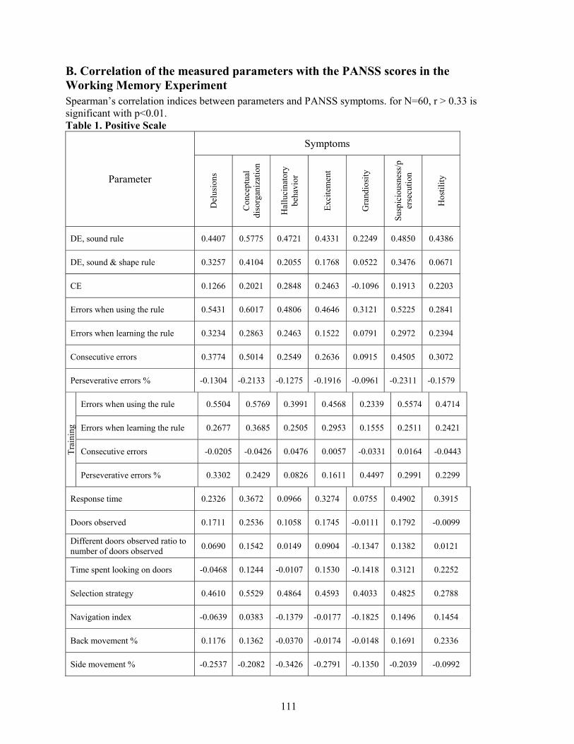
111
B. Correlation of the measured parameters with the PANSS scores in the Working Memory Experiment Spearman’s correlation indices between parameters and PANSS symptoms. for N=60, r > 0.33 is significant with p<0.01. Table 1. Positive Scale
Symptoms
Parameter
Del
usio
ns
Con
cept
ual
diso
rgan
izat
ion
Hal
luci
nato
ry
beha
vior
Exci
tem
ent
Gra
ndio
sity
Susp
icio
usne
ss/p
erse
cutio
n
Hos
tility
DE, sound rule 0.4407 0.5775 0.4721 0.4331 0.2249 0.4850 0.4386
DE, sound & shape rule 0.3257 0.4104 0.2055 0.1768 0.0522 0.3476 0.0671
CE 0.1266 0.2021 0.2848 0.2463 -0.1096 0.1913 0.2203
Errors when using the rule 0.5431 0.6017 0.4806 0.4646 0.3121 0.5225 0.2841
Errors when learning the rule 0.3234 0.2863 0.2463 0.1522 0.0791 0.2972 0.2394
Consecutive errors 0.3774 0.5014 0.2549 0.2636 0.0915 0.4505 0.3072
Perseverative errors % -0.1304 -0.2133 -0.1275 -0.1916 -0.0961 -0.2311 -0.1579
Errors when using the rule 0.5504 0.5769 0.3991 0.4568 0.2339 0.5574 0.4714
Errors when learning the rule 0.2677 0.3685 0.2505 0.2953 0.1555 0.2511 0.2421
Consecutive errors -0.0205 -0.0426 0.0476 0.0057 -0.0331 0.0164 -0.0443
Trai
ning
Perseverative errors % 0.3302 0.2429 0.0826 0.1611 0.4497 0.2991 0.2299
Response time 0.2326 0.3672 0.0966 0.3274 0.0755 0.4902 0.3915
Doors observed 0.1711 0.2536 0.1058 0.1745 -0.0111 0.1792 -0.0099
Different doors observed ratio to number of doors observed 0.0690 0.1542 0.0149 0.0904 -0.1347 0.1382 0.0121
Time spent looking on doors -0.0468 0.1244 -0.0107 0.1530 -0.1418 0.3121 0.2252
Selection strategy 0.4610 0.5529 0.4864 0.4593 0.4033 0.4825 0.2788
Navigation index -0.0639 0.0383 -0.1379 -0.0177 -0.1825 0.1496 0.1454
Back movement % 0.1176 0.1362 -0.0370 -0.0174 -0.0148 0.1691 0.2336
Side movement % -0.2537 -0.2082 -0.3426 -0.2791 -0.1350 -0.2039 -0.0992

112
Rotation movement % 0.4703 0.5169 0.3661 0.5052 0.2641 0.5236 0.3170
Errors when using the rule 0.3194 0.3119 0.1883 0.2460 0.1676 0.2624 0.2967
Errors when learning the rule 0.3341 0.3108 0.1780 0.2915 0.2009 0.2571 0.1574
Consecutive errors -0.2108 -0.1561 -0.0786 -0.1172 -0.1205 -0.1833 -0.1231
Perseverative errors % 0.1349 0.1328 -0.0341 0.0808 0.2122 0.1432 0.2363
Response time 0.2436 0.2368 0.0538 0.2584 0.3097 0.2486 0.3105
Im
prov
emen
t
Speed 0.3597 0.3436 0.2102 0.2501 0.2725 0.2560 0.2995
Table 2. Negative Scale Symptoms Parameter
Blu
nt a
ffec
t
Emot
iona
l w
ithdr
awal
Poor
rapp
ort
Pass
ive
/ ap
athe
tic
Diff
icul
ty in
ab
stra
ct th
inki
ng
Lack
of
spon
tane
ous
conv
ersa
tion
Ster
eoty
ped
thin
king
DE, sound rule 0.3074 0.3491 0.3054 0.3123 0.3507 0.2727 0.3000
DE, sound & shape rule 0.3417 0.3044 0.2750 0.3977 0.3879 0.3790 0.2269
CE 0.3737 0.3952 0.3867 0.3158 0.2919 0.3842 0.3635
Errors when using the rule 0.4592 0.4144 0.3678 0.4504 0.4592 0.3892 0.3302
Errors when learning the rule 0.3340 0.3291 0.2277 0.2968 0.3595 0.3600 0.2012
Consecutive errors 0.5716 0.5488 0.4508 0.5093 0.4963 0.5538 0.3797
Perseverative errors % -0.2390 -0.1878 -0.1388 -0.2364 -0.1759 -0.2058 -0.1545
Errors when using the rule 0.5975 0.5660 0.4931 0.5860 0.6269 0.5746 0.4197
Errors when learning the rule 0.2598 0.2966 0.3131 0.3106 0.4093 0.2041 0.2342
Consecutive errors 0.2438 0.2112 0.1667 0.1862 0.1278 0.2002 0.0226
Trai
ning
Perseverative errors % 0.1367 0.0915 -0.0140 0.0960 0.1062 0.0094 0.0887
Response time 0.5871 0.5603 0.5302 0.5293 0.3789 0.5588 0.4851
Doors observed 0.2840 0.2722 0.2320 0.2221 0.2649 0.3431 0.4075

113
Different doors observed ratio to number of doors observed 0.2733 0.2722 0.2240 0.1969 0.1704 0.3245 0.3525
Time spent looking on doors 0.3969 0.4029 0.4264 0.3991 0.3347 0.4012 0.2051
Selection strategy 0.3978 0.3863 0.3812 0.3982 0.4494 0.3142 0.3166
Navigation index 0.3529 0.3595 0.2860 0.3190 0.1762 0.4039 0.1962
Back movement % 0.2186 0.2154 0.1294 0.1844 -0.0198 0.1877 0.1153
Side movement % -0.2696 -0.2820 -0.3613 -0.2683 -0.3234 -0.2586 -0.3455
Rotation movement % 0.5317 0.5420 0.5826 0.4798 0.4972 0.4897 0.4071
Errors when using the rule 0.3597 0.3903 0.3553 0.3545 0.4283 0.3105 0.3288
Errors when learning the rule 0.1952 0.1596 0.1720 0.2334 0.2012 0.1554 0.2232
Consecutive errors 0.1057 0.0970 0.0869 0.0405 -0.0318 0.0809 -0.0109
Perseverative errors % 0.1598 0.1723 0.0801 0.0852 0.1363 0.0377 0.1274
Response time 0.2791 0.2543 0.2731 0.2260 0.2089 0.3628 0.2789
Impr
ovem
ent
Speed 0.2637 0.2337 0.2291 0.2618 0.1960 0.2861 0.2976

114
C. 10 best features chosen by different feature selection algorithms Mutual Information
Adding max info
RELIEF Simba (linear)
G-Flip (linear)
G-Flip (sigmoid)
error rate when the rule was used during training
error rate when the rule was used during training
error rate when the rule was used during training
error rate when the rule was used during training
complexity effect
consecutive error rate
response time
response time
consecutive error rate
door looking time
error rate when the rule was used
error rate when the rule was used during training
rotation movements
distractor effect (sound and shape rule)
error rate when the rule was used
consecutive error rate
error rate when the rule was used during training
consecutive error rate during training
door looking time
consecutive error rate during training
Selection strategy
Side movements
consecutive error rate during training
selection strategy
consecutive error rate
perseverative error rate during training
error rate when learning the rule
number of different doors observed
door looking time
side movements
distractor effect (sound and shape rule)
error rate when learning the rule
improvement in error rate when learning the rule
error rate when learning the rule during training
navigation index
improvement in error rate when the rule was used
perseverative error rate during training
improvement in navigation speed
back movements
improvement in consecutive error rate
side movements
consecutive error rate during training
improvement in response time
error rate when learning the rule during training
back movements
improvement in navigation speed
error rate when learning the rule
number of doors observed
distractor effect (sound rule)
improvement in response time
error rate when the rule was used
perseverative error rate
consecutive error rate during training
rotation movements
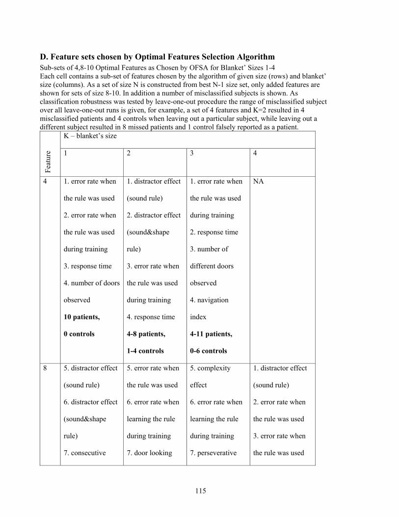
115
D. Feature sets chosen by Optimal Features Selection Algorithm Sub-sets of 4,8-10 Optimal Features as Chosen by OFSA for Blanket’ Sizes 1-4 Each cell contains a sub-set of features chosen by the algorithm of given size (rows) and blanket’ size (columns). As a set of size N is constructed from best N-1 size set, only added features are shown for sets of size 8-10. In addition a number of misclassified subjects is shown. As classification robustness was tested by leave-one-out procedure the range of misclassified subject over all leave-one-out runs is given, for example, a set of 4 features and K=2 resulted in 4 misclassified patients and 4 controls when leaving out a particular subject, while leaving out a different subject resulted in 8 missed patients and 1 control falsely reported as a patient.
K – blanket’s size
Feat
ure 1 2 3 4
4 1. error rate when
the rule was used
2. error rate when
the rule was used
during training
3. response time
4. number of doors
observed
10 patients,
0 controls
1. distractor effect
(sound rule)
2. distractor effect
(sound&shape
rule)
3. error rate when
the rule was used
during training
4. response time
4-8 patients,
1-4 controls
1. error rate when
the rule was used
during training
2. response time
3. number of
different doors
observed
4. navigation
index
4-11 patients,
0-6 controls
NA
8 5. distractor effect
(sound rule)
6. distractor effect
(sound&shape
rule)
7. consecutive
5. error rate when
the rule was used
6. error rate when
learning the rule
during training
7. door looking
5. complexity
effect
6. error rate when
learning the rule
during training
7. perseverative
1. distractor effect
(sound rule)
2. error rate when
the rule was used
3. error rate when
the rule was used
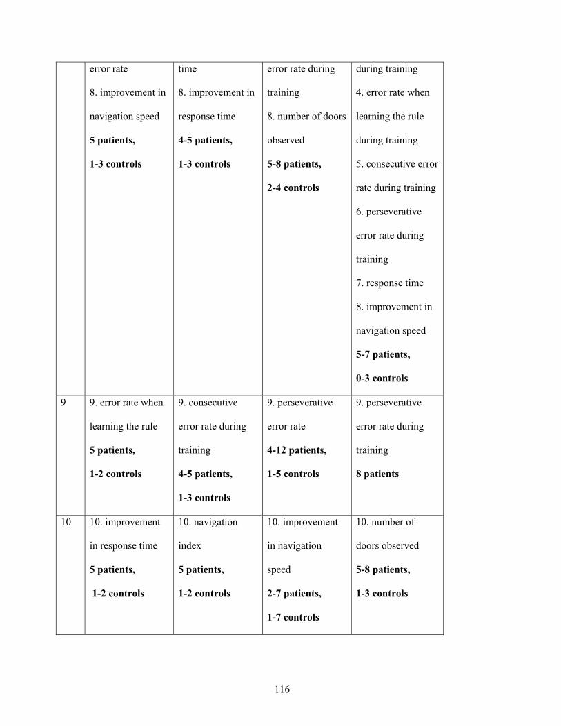
116
error rate
8. improvement in
navigation speed
5 patients,
1-3 controls
time
8. improvement in
response time
4-5 patients,
1-3 controls
error rate during
training
8. number of doors
observed
5-8 patients,
2-4 controls
during training
4. error rate when
learning the rule
during training
5. consecutive error
rate during training
6. perseverative
error rate during
training
7. response time
8. improvement in
navigation speed
5-7 patients,
0-3 controls
9 9. error rate when
learning the rule
5 patients,
1-2 controls
9. consecutive
error rate during
training
4-5 patients,
1-3 controls
9. perseverative
error rate
4-12 patients,
1-5 controls
9. perseverative
error rate during
training
8 patients
10 10. improvement
in response time
5 patients,
1-2 controls
10. navigation
index
5 patients,
1-2 controls
10. improvement
in navigation
speed
2-7 patients,
1-7 controls
10. number of
doors observed
5-8 patients,
1-3 controls

1
בסכיזופרניה הפרעות של אבחונית הערכה עבור מדומה מציאות
חיבור לשם קבלת תואר דוקטור לפילוסופיה
מאת
אנה סורקין
בירושלים, הוגש לסנט האוניברסיטה העברית 2006 אוקטובר

2
:העבודה זו נעשתה בהדרכתה של
דפנה ווינשל' פרופ

1
תקציר
למחלה אין סממן גנטי או ביולוגי . סכיזופרניה הינה מחלת מוח קשה שמורכבת מתסמינים רבים ומגוונים
כל חולה מבטא מכלול . כיאטרי ומתבסס על ביטוי התסמיניםואבחון הסכיזופרניה מתבצע על סמך ראיון פסי
עובדות אלו מקשות על . ואין אף תסמין ייחודי למחלה או שמתבטא בכל החולים, שונה של תסמינים
יחד עם זאת אבחון מוקדם ומדויק . האבחון כך שאבחון הסכיזופרניה הינו תהליך סובייקטיבי ואף לא אמין
. בחולים סכיזופרנייםתווך ארוךהנזקים התפקודיים לצמצום קריטי לגורם הינו
לצורך פיתוח , מציאות מדומה בפרט ,כלים טכנולוגיים מתקדמים מתמקד בפיתוח ושימוש בשליהמחקר
לבסס קודם כל אני מציעה. סת על שלושה מרכיבים מתבסהגישה שלי. ת לאבחון הסכיזופרניהגישות חדשו
שיאספו בעת ביצוע של ם מדדים אובייקטיבייולכלי קוגניטיבי תפקודי שאת אבחון הסכיזופרניה על פרופיל
לפגיעה באינטגרציה בין מערכות עצבים במוח כגורם מרכזי אני מתייחסת, שנית.מבחנים קוגניטיביים
יביים שמאתגרים על מבחנים קוגניט ולכן פרופיל אבחוני של סכיזופרניה צריך להסתמך ,לסכיזופרניה
מודלית- במציאות מדומה על מנת ליצור סביבה ניסויית רבאני משתמשת, ולבסוף. רציהתהליכי אינטג
.שמאפשרת ביטוי ללקויי האינטגרציה ומדידתם
בפרופיל האבחוני של לחקרתי שני מימדים קוגניטיביים שצריכים להיכל, כדי להשיג את המטרות האלה
היות והזיות שמיעתיות הינן התסמין . סת המציאותאינטגרציה תחושתית בזיכרון העבודה ותפי: סכיזופרניה
ברמות יה ראיבין אופנויות השמיעה והבחרתי לחקור אינטגרציה , הפסיכוטי החמור ביותר בסכיזופרניה
הנבדק בו,ברמה נמוכה של אינטגרציהמתמקד העבודה ןזיכרו לפי כך הניסוי של .קוגניטיביות שונות
הניסוי של תפיסת המציאות דוגם כאשר . מ לצאת ממבוך"צורה עצבע ו, נדרש לזכור שילוב של צליל
- אי שלדורשת זיהוישמטה במשימה -עלהמעלה ומ-יה קונספטואלית המשלבת תהליכים מטהאינטגרצ
העלים על , בו החתול נובח, מציאות מדומה שלבניסוי הזה המשתתף מנווט בעולם. התאמות בסביבה
התאמות בין אופנויות של ראייה -ם אלה יוצרים אייאירוע. בתחנההעצים אדומים ופרות מחכות לאוטובוס
.התאמות של צבע ומיקום-ושמיעה ובתוך אופנות הראייה אי

2
את המשתתפים לחולי סכיזופרניה וביקרות בהתבסס על השמפרידבי פתחתי פרוצדורה לכל מימד קוגניטי
שילוב של שני . של החולים85-88%ו נכון וניבא, שני המימדים הראו יכולת ניבוי גבוה. בניסויתפקודם
. כפי שהודגם בחולים הסכיזופרניים שנבחנו על שני המימדים, המימדים משפר את הניבוי עוד יותר
עם מדדים אבחוניים סטנדרטיים מעידה על פוטנציאל תפקודייםמספר של מדדים קורלציה מובהקת של
.התפקודייםאבחוני של המדדים
מ לאפיין את ההפרעות הרבות "ע. מסגרת לפיתוח של פרופיל אבחוני של סכיזופרניהמגדירהמחקר הזה
יכולת כמו למשל, ם נוספיםשל הסכיזופרניה הפרופיל האבחוני הסופי צריך לכלול מימדים קוגניטיביי
. חברתיתה ואינטראקציי אמוציונאל מימד,למידה

3
תוכן העניינים
1פרק
בואמ
1...........................................................................................................סכיזופרניה 1.1
3...............................................................................כפגיעה באינטגרציה סכיזופרניה 1.2
9..................................................................................תפקוד קוגניטיבי בסכיזופרניה 1.3
14.....................................................................................................בעיית האבחון 1.4
15........................................................................פרופיל אבחון של סכיזופרניה: גישה 1.5
19................................................................................................... התוצאותיתווא 1.6
2פרק
שיטות המחקר
20................................................................................................................מטרה 2.1
21.....................................................................................................פיתוח ניסויים 2.2
22...........................................................................................פיתוח מציאות מדומה 2.3
26.......................................................................................................אלגוריתמים 2.4
3פרק
זיכרון העבודה
31...................................................................................זיכרון העבודה: 1' ניסוי מס 3.1
55.........................................................................................פרזוורציה: 2' ניסוי מס 3.2

4
4פרק
תפיסת המציאות
60........................................................................תפיסת המציאות בחולי הסכיזופרניה 4.1
89...........................................................שילוב של שני מימדים של הפרופיל האבחוני 4.2
92.............................................................השוואה עם מבחנים קוגניטיביים סטנדרטיים 4.3
5פרק
שמיעתית בנבדקים בריאים-אינטגרציה ראייתית
93........................................................................שמיעתית בנבדקים בריאים-ינטגרציה ראייתיתא
6פרק
דיון ומסקנות
99.....................................................................................................................דיון ומסקנות
103.....................................................................................................................יבליוגרפיהב
נספחים
A .110....................ריגה מתווך התקין בקרב חולי סכיזופרניה וקבוצת ביקורת בניסוי זיכרון העבודהח
B .ורלציה של המדדים הניסויים עם ציוני הק-PANSS111..............................כרון העבודה בניסוי זי
C .10 114.............................י אלגוריתמים שונים לבחירת תכוניות"מדדים הכי טובים כפי שנבחרו ע
D .י האלגוריתם "מדדים שנבחרו עOFSA............................................................................115