Virtual Mass

Technique for Computing

Space Trajectories

Final Report

(ACCESSION (THRU}

(PAGES) ( DE)

(NASA CR OR TMX OR AD _IUMBER) (CATEGOR f|

I

!

GPO PRICE $

CFSTI PRICE(s) $ ; " " "

Hard copy (HC) ,

Microfiche (MF) "17/_-_

ff 653 July 65

,ll,,ir_ R'rl

i i i i i i ii i i ilrllll i i ii ilrll i iin i i inUlll illlnlll.l.l,nlln|.lll ii ii ill

1966009743

//

Virtual Mass

Technique for Computing

Space Trajectories

Final ReportP

Contract No. NAS 9-4370

ER 14045

January 1966

by D. H. Novak

M_I _ 7"1/I/i_' BALTIMORE DIVISION

BALTIMORE,MARYLAND 21203

i

1966009743-002

1I

!

i

!

!

tFOREWORD

I The work described in this report was performed by the MartinCompany for the NASA Manned Spacecraft Center under ContractNo. NAS 9-4370.

ER 14045iii

1966009743-003

/

CONTENTS

Page

Foreword .............................. iii

Summary .............................. vii

I. Introduction ............................ 1

II. Basic Principles of the Virtual Mass ............ 3

A. Review of the Restricted Three-Body Problemin Terms of the Gravisphere .............. 3

B. Generalization of the Gravispheric Force Center jConcept to the Case of More Than Two Gravi-tating Bodies ......................... 6

C. The Solution of the N-Body Problem as Viewed fin the Light of the Virtual Mass ........... 10

III. Digital Computation Formulational Considerations... 15

A. Vector Orbital Elements ................. 15

B. Noniterated Versus Iterated Computation ...... 22

C. The Computing Interval .................. 24

IV. Digital Computer Study ..................... 29

A. Approach ........................... 29

B. Results ............................ 30

V. General Description and Use of the Virtual Mass Pro-gram for Computing Space Trajectories .......... 41

A. General Descriptior, .................... 41

B. Input and Output ....................... 43

C. Sample Problem ...................... 46

ER 14045V

1966009743-004

CONTENTS (continued)

Page

VI. Details of the Computer Program .............. 67

A. Flow Diagrams ....................... 67

B. Array Notation ....................... 71

C. FORTRAN IV Listing of Program ........... 73

VII. Conclusions and Recommendations ............. 91

A. Conclusions ......................... 91

B. Recommended Further Studies ............. 9i

VIII. References ............................. 93

ER 14045vi

1966009743-005

This study has demonstrated the feasibility of the Virtua! MassTechnique for computing space trajectories and has developed aFORTRAN IV digital computer program for solving the restrictedthree-body problem by this procedure. The virtual mass at any in-stant of time replaces the combined gravitational effects of all thereal celestial bodies upon a spacecraft. The magnitude and locationof this fictitious body, along the line of the instantaneous resultantforce vector, are uniquely computed by formulas derived from thegeneralization of the gravispheric force center concept. The compu-tational procedure is based upon the assumption that, over a smalltime interval, the spacecraft motion can be represented as a two-body conic section arc relative to the moving and varying virtual mass.In this manner the complete trajectory is computed as a series of sucharcs, pieced together in a stepwise manner--updating the position andmagnitude of the apparent force center at each step. Thus, the virtual jmass technique is like the patched conic approximation in that no differ-ential equations are integrated numerically. It is similar to theCowell method in that the equations for the virtual mass are much likethe acceleration contribution terms in the differential equations of mo-tion. As the spacecraft nears one of the real physical bodies, thoseterms dominate the contributions of the other bodies and the effective

force center approximates that real body in size and location. Finally,this technique displays a kinship to the Encke method in the computa-tion of a reference trajectory relative to the dominant body. Thisdominating body, however, is the continuously moving and varyingvirtual mass rather than one of the physical bodies. Since the perturb-ing effects of all bodies are included in the determination of this ap-parent force center, effectively a perfect rectification is made at eachstep and there is no need to numerically integrate these perturbations.

A single compact computer program embodying this procedure canbe controlled very simply to compute an approximate solution rapidlyas a series of relatively few patched conics or a highly accuratetrajectory as a large number of such arcs at the expense of propor-tionately longer computation time. For example, a 70.33-hr insertion-tolpericynthion circumlunar trajectory was computed (and a largeamount of output data were printed) in 160 seconds on an IBM 7094computer. This trajectory gave the spacecraft position at pericynthionaccurate to within 0.02 naut mi and exhibited a total variation of the

Jaccbi energy of less than 2 parts out of 7 x 106. __I_/_(_)

t ER 14045vii

.JL

1966009743-006

I

BLANK PAGE

1966009743-007

/

I. INTRODUCTION

It is well known that there is no closed-form general solution for thetrajectory of an infinitesimal spacecraft freely falling in the combinedgravity fields of two or more large celestial bodies. Therefore, eachcase must be solv,_d individually by an approximate numerical proce-dure. Currently, two alternative procc.dures are used for finding suchsolutions; namely, the patched conic approximation technique and theaccurate numerical integration of the differential equations of motion.

'fhe patched conic technique makes the simplifying assumption that,while the spacecraft is within the sphere of influence of any gravitatingbody, the motion is dominated by that large body to the complete ex-clusion of all others. Since the general solution to the two-body prob-lem is known to be a Keplerian conic section, a crude app:oximationto the n-body solution can be computed as a series of thes,: preintegratedconic sections, patched together appropriately at the boundaries of the ,_spheres of influence.

The precise numerical solution of the differential equations involves trather laborious step-by-step computation procedures, based upon oneof two fundamental approaches.

The straightforward method of Cowell treats all terms in thedifferential equations as contributors of equal importance. Most ofthe time, however, the acceleration experienced by the infinitesimal

body is dominated by a single one of the gravitating bodies, and allother contributions are small by comparison. This requires that greatcare be exercised when combining all the terms so as not to lose thesignificance of the small contributions. This computational difficulty

_::i tends to offset the advantage of the formulational simplicity of this method.

" The other basic approach (due to Encke) consists of recognizing'/

this domination of the motion by one body and computing the trajectory!_ in two stages. First, the position and velocity at some time (epoch)

are considered to define the elements of the osculating Keplerian conic

section relative to the dominant body. Then, the perturbing relativeaccelerations of the less influential bodies are numerically integrated,f_carrying comparatively few significant digits, to obtain the path correc-

*' tion to be applied to the basic Keplerian motion. As the magnitude ofthe perturbed motion grows larger, accuracy would be lnst withoutcarrying more significant figures. Instead, when this h___pens, the

11 II

reference conic section is rectified to obtain new osculating elementsat a later epoch, thus reducing the magnitude of the perturbations.

This procedure works well for the case where the motion is alwaysdominated by one particular body, as is the case for the planetarymotions about the sun. Spacecraft on lunar or interplanetary trajectories,

ER 140451

1966009743-008

on the other hand, traverse from one sphere of inf!;_ence to another--falling under the domination of successively different reference bodies.During the transitions from one reference body to aoother, the opace-craft is literally torn between the two major attractions. Sophisticatedlogic is required to enable the computer to select the dominant bodyand to switch from one reference body to another to ensure that thiscomputational discontinuity does not disturb the co,_tinuity of the tra-jectory being integrated.

This sophistication is generally considered worthwhile, for theEncke integration step size can be much larger than that of the Cowellmethod. The final selection of one or the other probably is more amatter of personal preference, however, since the Cowell step can bebe executed much faster.

Regardless of which integration procedure is used, the solutionmethods described offer the choice betw,,:en a very crude, rapidlycomputed, patched conic trajectory and a high precision comparativelyslow- running integrated solution. The former type is useful forparametric studies and early mission planning purposes to determineapproximate injection conditions. The latter is needed for the re-finement of rough initial conditions into an accurate determination of h_:the requirements for a spec.!_c n::_zsion. Aside from the fact thattwo different programs are needed, this refinement process may in-volve iterative computation w._,th the accurate but slow-running pro-gram. This is due to the wide gap between the crude approximationand the precision soluLion and to the very high sensitivity of spacetrajectories to errors in initial conditions.

This report des bes a unique method of conmuting n-body tra-jectories which off, rs, in a single digital compa!:, r program, thecapability of efficiently covering the ccmplete s!,uctrum from rapidcrude solutions to more time-consuming accu_'a,,_c solutions. ChapterII describes the basic concept upon which the :',_nputation is based,and Chapter III discusses various consider:,_i,,as which must be madein mechanizing this concept for digital co_,,_:,,_:ation. Chapter IV pre-sents the quantitative results of the stud:,, :,_' these considerations, there-by showing how these items have been implemented. Chapter V givesa general description of the computer program and complete instruc-tions in the use of it. For the reader who is interested or who desires

to make changes for his own requirements, a detailed description isgiven in Chapter VI, including a complete FORTRAN _'sting of the program.

ER 140452

1966009743-009

^

II. BASIC PRINCIPLES OF THE VIRTUAL MASS

The concept of the virtual mass is based upon the idea of replacingthe colnbined gravitational effects of many large celestial bodi" s uponan infinitesimal spacecraft by the attraction of a single equivalent body.This fundamental idea is not new. Its natural applicability to the re-stricted three-body problem (two large masses and one infinitesimal .-mass} is described in Refs. 1 and 2. A rather arbitrary attempt wasmade to make a similar reduction of the r-body problem in Ref. 3. Thelatter consisted of singling one point out of thp. infinite number of possi-bilities along the line of the in_tantaneet, s resultant gravitational forceon the vehicle. Once the location (assumed inertially fixed} was chosen.of course, the mass magnitude was determined to give the correct _orce.T?,e virtual mass location and magnitude, dercribed in this reporthowever, are derived as the n-body generalization of the gravisphericforce center associated with the restricted three-body problem. There-fore, the presentation begins with a brief review of what is already knownabout the restricted three-body problem and proceeds from there withthe generalization to the case of more than two gravitating bodies.

[

A. REVIEW OF THE RESTRICTED THREE-BODYPROBLEM IN TERMS OF THE GRAVISPHERE

Consider the simple system comprised of only two large magnitude

point masses _I and _2 and (by comparison) an infinitesimal mass

spacecraft S. The designation of the mass by the symbol F is intendedto suggest that the real quantity of interest is the mass ti:nes the Uni-versal Gravitation Constant. The locus of all spacecraft positions S

w_'_,h constant ratio p of distances rls, r2s to the two masses is a

spherc with center G on the i._ne through _I and 'a2 as shown in Fig. I.

Since the gravitational attraction depends only upor, displacement from ____._.the mass, the ratio of the gravitational attractions is also constant onsuch a spherical surface; hence, it is called a gravisphere.

The gravisphere exhibits an interesting intrinsic physical property;

namely that, for all points on its surface, the resultant F R of the at-

tractions F 1, F 2 of the two bodies passes through a single focal point

V on the line between _1 and _2 as shown in Fig. 2. The location of

V relative to _1 can be shown (e. g. from relations derived in Ree. 2)to be

ER 140453

1966009743-010

_23

_. -. r2s

rvl = r21 _1 _2--_ +---y

r

rl_ -2s

where

r.. = r. - r.lj 1 J

The location of this gravispheric force center can also be expressedrelative to the same frame to which tbe masses are referred:

u 23

r 2r = r 1 + -- r 1 +(r 2- r 1)

v rvl _1 _23 + 3

rls r2s

or

_Ir I _2 r2_-+ 3

.. rls r2sr -- (II- 1}

v _1 _2_+ 3

rls r2s

The magnitude of the effective mass (times Universal Gravitation

Constant} _v _.hich must be concentrated at V to replace the combined

effects F R of _1 and _2 also can be derived from expressions given inRef. 2 as

v - rvs 3 + 3 (II-2)rls r2s

Note that, unlike the fixed focal point location, the grav£spheric massmagnitude varies according to the radial displacement r of the pointon the surface from V. vs

ER 140454

1966009743-011

S . lsGravtsphere: 0- r-- -- constant

2s

/ _,oi_-'""-..r_s'"r I. 21 # #- _ "'.- "-

" " 2S ""--.. "..

/ I ,"r_s --..---..l e/' ""-,....'.,-...

O gl _12

Fig. 1. Illustration of a Gravisphere

_S "* /------ Oravisphere:

_2 _ O-- rls =constant

.- / ':_. \ _ rTs: "7 ?s/ --- ---

-" _V ] _2 -G _1 rvl

Fig, 2. The Gravispherie Force Cen":er

Ix2,_ U5/ f

/ /

ii / /

l.l 1 __

$S _

Fig. 3. Extension of Gravispheric Force Center Concept to More than Two Bodies

ER 140455

i

1966009743-012

These considerations show ho_ the attractions of two masses on aninfinitesimal spacecraft can be reduced to the instantaneously equivalentattraction of a single mass. The magnitude and location of this equiva-lent mass on the line between the gravitating masses can be easily com-

puted from equations {II-1, 2), knowing r s, r 1, r 2, _1 and _2" Observe

that when the spacecraft is ',.quidistant from both bodies rls - r2s and Eq

(II-1) reduces to the usual expression for the center of mass. Thus,only in this case does the gravispheric force center coincide with thebarycenter. (In this case the gravisphere is the plane dividing the space

between _1 and _2' ) Note also that the mass magnitude equals the totalof the two real masses when the spacecraft is infinitely far displaced.

B. GENERALIZATION OF THE GRAVISPHERIC _ORCECENTER CONCEPT TO THE CASE OF MORE THAN

TWO GRA\rITATING BODIES

Extension of the concept of the gravisphere itself to the case of threeor more bodies is impossible. Except under very special circumstances,there simply are no surfaces of constant ratios of distances or gravita-tional attractions. However, now that the expressions (II-1) and (II-2)have been derived, it is no longer necessary to think in terms of thesesurfaces used in the derivation. The simpler condition expressed bythese relations suggests the method by which the concept can be extended

: to n bodies. Consider the geometry sketched in Fig. 3. First select

any two masses (say _1 and _2 } and via Eqs (II-1 and 2) replace themby an equivalent mass appropriate to the spacecraft position relative tothem. Now take this fictitious mass and another one ef the real gravi-

tating bodies (_3' say} and replace these two by a new fictitious mass.Continue this process, stepping around the system, until all gravitatingrnasses have been replaced by a single equivalent mass.

This geometric description can be expressed analytically by a straight-f,_rward application of the formulas (II-1, 2). The first step, of course,yields .,

_lrl ._2r2+

3 3-. rls r2sr

v12 _1 _2+3 3

rl s r2 s

ER 140456

1966009743-013

- r 3 + 3v12 v12 s r r2s

where the subscripts 12 indicate that these values obtain for masses

ILl' _2" Now again apply the basic formulas, treating _v as _112

r as r 1 and % as _2' r3 as r2:v12 ..

r % r3_v12 v123 _ + 3

rvl2 s r3s--* Jr =

v123 _v!.2 _33 + 3

rvl2 s r3s

ILl rl _2 r2 _3 r3+ +3 3 3

rls r2 s r3s

_i _2 _3+ +

3 3 3rl s r2 s r3s

3( v12- r 3 + 3

_v123 v123 s rvl2 s r3s

3 ( _1 _2 _3 )

= r

V123 s 3 + 3 + 3rls r2s r3s

With repeated application of the procedure, one gets for n gravitatingbodies:

ER 140457

1966009743-014

-_ Mr -

v MS

3= r M s_V VS

where

n __ > (II-3)-_ _ _i riM = _a 3ris

i=l

n

Ms-- 3i = 1 ris

and where

_i - mass of ith gravitating body (times Universal GravitationConstant)

r i = position of ith gravitating body

r s = position of spacecraft

-- r. - rris I S

= r - rrvs v s

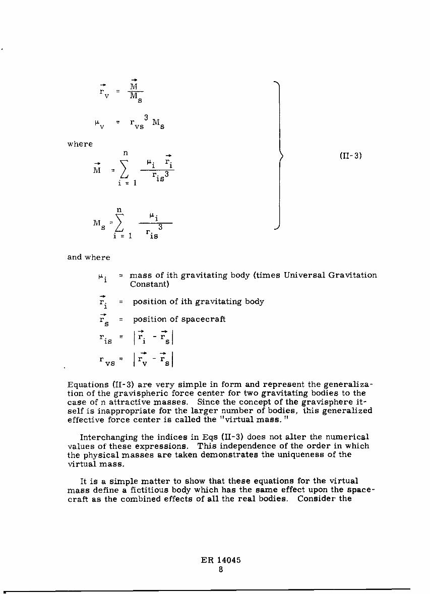
Equations (II-3) are very simple in form and represent the generaliza-tion of the gravispheric force center for two gravitating bodies to thecase of n attractive masses. Since the concept of the gravisphere it-self is inappropriate for the larger number of bodies, this generalizedeffective force center is called the "virtual mass. "

Interchanging the indices in Eqs (II-3) does not alter the numericalvalues of these expressions. This independence of the order in whichthe physical masses are taken demonstrates the uniqueness of thevirtual mass.

It is a simple matter to show that these equations for the virtualmass define a fictitious body which has the same effect upon the space-craft as the combined effects of all the real bodies. Consider the

ER 140458

1966009743-015

,/

vector differential equation of motion of the spacecraft:

n

_- i (ri rs)s 3

i = 1 ris

This equation can be written as

n

-k" n _ti ri "* _ir s r 3r. 3 s r.

i = 1 is i = 1 is •

= M - r s M s

by Eq (II-3c, d). By Eq (II-3a, b) it becomes

-_ _. PLv -.rs = Ms (rv- rs) = 3 rvsr

vs

Thus, the virtual mass acceleration of the spacecraft is identical withthe acceleration by the real gravitating bodies.

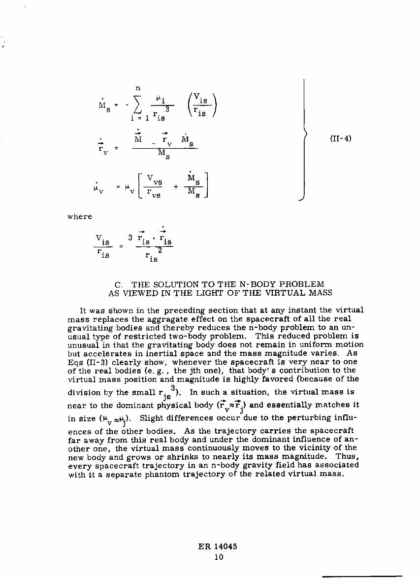
Equations (II-3) can be differentiated to give the velocity and massrate of the virtual mass as functions of the positions and velocitiesof the spacecraft and the gravitating bodies:

-%

• _ _ i r. r. Visi = 1 ris (II-4)

ER 140459

i

1966009743-016

n

Ms-- 3 \ris /i-- lris

2,. ..,.• M r M (II-4)

-_ - V S

rv MS

tXv = _'v + Mrvs s

where4

V. 3r. .r.iS IS IS

r.is r.

1S

C. THE SOLUTION TO THE N-BODY PROBLEMAS VIEWED IN THE LIGHT OF THE VIRTUAL MASS

It was shown in the preceding section that at any instant the virtualmass replaces the aggragate effect on the spacecraft of all the realgravitating bodies and thereby reduces the n-body problem to an un-usual type of restricted two-body problem. This reduced problem isunusual in that the gravitating body does not remain in uniform motionbut accelerates in inertial space and the mass magnitude varies. AsEqs (II-3) clearly show, whenever the spacecraft is very near to oneof the real bodies (e. g., the jth one), that body' s contribution to thevirtual mass position and magnitude is highly favored (because of the

division by the small rjs3). In such a situation, the virtual mass is

near to the dominant physical body _rv_rj; and essentially matches it

in size (_v =_j)" Slight differences occur due to the perturbing influ-ences of the other bodies. As the trajectory carries the spacecraftfar away from this real body and under the dominant influence of an-other one, the virtual mass continuously moves to the vicinity of thenew body and grows or shrinks to nearly its mass magnitude. Thus,every spacecraft trajectory in an n-body gravity field has associatedwith it a separate phantom trajectory of the related virtual mass.

ER 1404510

1966009743-017

/

A simple example of this behavior is illustratedin Fig. 4. Thetrajectories shown are for the restricted three-body problem, wherethe two-dimensional circumlunar spacecraft trajectory is flown in theearth-moon orbital plane, Of course, for this case of only two gravitat-ing bodies, the virtual mass motion is restricted along the earth-moonline. The two paths are depicted as the solid lines in an inertiallyoriented barycentric coordinate system. The moon trajectory is shown,however, the earth motion has been omitted to keep the curves un-cluttered near the origin. Relative position lines between the virtualmass and the spacecraft are shown at several time points by the dashedlines. To the scale of the plot, the initial virtual mass disp]acementfrom the center of earth is indistinguishable. Note also that the virtualmass coincides with the bacycenter at approximately 22 hr, where thespacecraft is equidistant from earth and moon. Figure 5 shows thecorresponding variation of the virtual mass magnitude for this example.The abscissa is the virtual mass displacement along the earth-moonline. Time points corresponding to those appearing in Fig. 4 are spotted j,,on the curve.

Of course, the idea is immediately suggested of using the virtualmass as a means of constructing the spacecraft n-body trajectory in astepwise numerical procedure. Consider that the spacecraft positionand velocity are given in some reference frame at some instant of time.Assume also that an ephemeris gives the positions and velocities of thegravitating bodies (of known masses) in this same reference frame.These data are sufficient to compute the virtual mass position, velocity,mass magnitude and magnitude rates from Eqs (II-3) and (II-4). Thenby simple subtractions, the spacecraft position and velocity vectorscan be computed relative to the virtual mass at this instant of time.If now the relative motion is computed over some increment of time,the spacecraft trajectory can be propagated and transformed back tothe reference coordinate frame. The whole process can now be re-peated with the new position and velocity of the vehicle at the new time.

If the virtual mass were fixed in magnitude and unaccelerated, onecould compute the spacecraft relative motion over any finite arc withno error as the conic section solution to the two-body problem. Theabsolute motion would be exact as well for this case where the fixed

magnitude virtual mass moves with constant velocity. The mass andvelocity do change, however, and hence, the characterizations of thespacecraft relative motion as a conic section and of the virtual massmagnitude and velocity as constant are not exact. But this is nodifferent from any other approximation scheme associated with thenumerical integration of differential equations. The fundamentaltheorem of the calculus guarantees that theoretically, the errors ofthis approximation will vanish in the limit as the arc length (time in-crement) approaches zero. There is, of course, a practical limit tothe accuracy which can be achieved due to the limitation of the number

ER 14045II

l

1966009743-018

#

220 - _ 6569.31 60 55 50 45

20O 65__30

oo \_o_.,.°° _oon._o_,,--_ "_0 _

160 _\40_

Virtual mass trajectoryt

140 35_

30_ 55

120 I0- 25'X

lO0 - l

80 1

I

/ lo60 I

/I

40

I ,

_0/ craft trajectory2O

II35,

-201 I | ] | I t I

-20 20 40 60 '80 I00 120

X I (naut mix 103 )

Fig. 4. Virtual Mass Trajectory for an In-Plane SpacecraftTrajectory

ER 14045

12

1966009743-019

CDO II

v

cH ._

L_ C_j c_

o :> .

.Ms., _..,=4

LP_

°/

'_ o

E___ , , i I, ,, , , , , i lil l i i i i I

,-; d

(zaq/£!_a _,n'eU)oi_Ol x'^rf '(_,suoo .,-'e.xO Tuff x) opnlTu_'eN 9_eN I'_n_,aTA

ER 1404513

1966009743-020

of digits which can be carried in the computations and the length oftime available to perform them. The next two chapters will treat thesepra3tical aspect,_ of the numerical calculation.

This chapter will be concluded with some observations concerningthis new procedure for solving the n-body problem. There is a simi-larity to the Cowell method in the procedure of adding up the attrac-tions of all the real gravitating bodies at each computing step (seeEqs (II-3)). This summation, however, is not expressed in terms ofthe resultant force; but rather as the magnitude and location of a"virtual mass" which instantaneously produces identically the sameresultant force on the spacecraft. It is like the Encke procedure inthat a Keplerian conic section is computed relative to the virtual massas the reference body. Of course, there are no discontinuous jumpsfrom one reference body to another, since the virtual mass movescontinuously from the vicinity of one real body to that of another asthe spacecraft trajectory is dominated by successively different bodies.Since all the perturbing effects are included in the computation of thevirtual mass, a perfect rectification is made at each computing inter-val. This then eliminates entirely the need for numerically integratinghigher order acceleration perturbations. Thus, finally, the procedureis like the patched conic technique in that only preintegrated conic sec-tion solutions are pieced together.

ER 1404514

1966009743-021

III. DIGITAL COMPUTATION

FORMULATIONAL CONSIDERATIONS

It has been truly said that numerical computation is more of an artthan a science. This Chapter in fact is an exposition of a p: imitiveform of the art practiced here to implement the concel-ts discussed inthe last Chapter in a digital computer program. Where alternativeapproaches and variable mechanizations are described here, they weretested and compared in the computer. The results are l eported in thefollowing Chapter.

A. VECTOR ORBITAL ELEMENTS

A number of complications and inefficiencies _culd result if thecomputation scheme outlined in the preceding Chapter were implementedin terms of the conic section equations as generally written in polarcoordinates in the p',ane of motion. The complications would arise inthe special procedures required to handle cases of zero inclination,zero eccentricity and unity eccentricity. The principal inef¢iciencywould manifest itself in the necessity for a large number of coordinatetransformations. Each computation cycl_, would requir_ a rotationaltransformation from the reference (ephelner's} frame to the instantar, eousplane of motion, defined by the position and velocity relative to thevirtual mass, and back again.

Tile tr isformations can be eliminated entirely and the other dif- _ficulties qinimized by using the three-dimensional vector formulationof the two-body conic section solution. These relations will be de-veloped here for the sake of including in this report a complete listingof the equations required for the computation.

If both sides of the vector equation of motion for the two-bodyproblem: *

(Iii- 1)r = 3

£

are cross-multiplied by r, the equation

rxr= --_ rxr = 0results, r

*The quantities are not subscripted here for the sake of simplicity ofnotation, it is to be ,,nderstood, nevertheless, that the spacecraftmotion relative to the virtual mass is implied.

ER 1404515

1966009743-022

This can be integrated to obtain

k = r x r (III-2)

The constant of integration_"willbe called the "kepler vector" sinceitobviously represents twice the areal rate. Now form the vectorproduct of Eq (III-2) and Eq (III-1), divided by -u:

(_'x x r1 -*kxr=

U 3r

d (rr_._)and hence thisIt can easily be shown that the right side is _-

equation can be integrated to yield

-_ r kxre = (III- 3 )r

This integration constant _" will be called the "eccentricity vector. "

The magnitude of _* is the eccentricity of the conic section and thevector points along the major axis toward periapsis.

The equation of the conic section is easily derived from Eq (III-3)

by forming its inner product with r.

-_ -_ r _ kxr -_e.r- ...... rr t_

Interchanging the dot and cross in the last term on the right and sub-stituting from Eq (III-2) gives finallj

-. .. k 2e.r - -r + _ (III-4)

Actually Eq (III-4) defines a three-dimensional surface rather than apath. The orbit is specified as the intersection of this surface with

the plane normal to k.

The velocity r can easily be determined at any position r on a given

orbit k, e. Observe first that since k is orthogonal to r:

k &-ff-xr

is a vector in the plane of motion, perpendicular to the velocity vectorand equal to it in magnitude. The cross product of this resulting vector

ER 1404516

1966009743-023

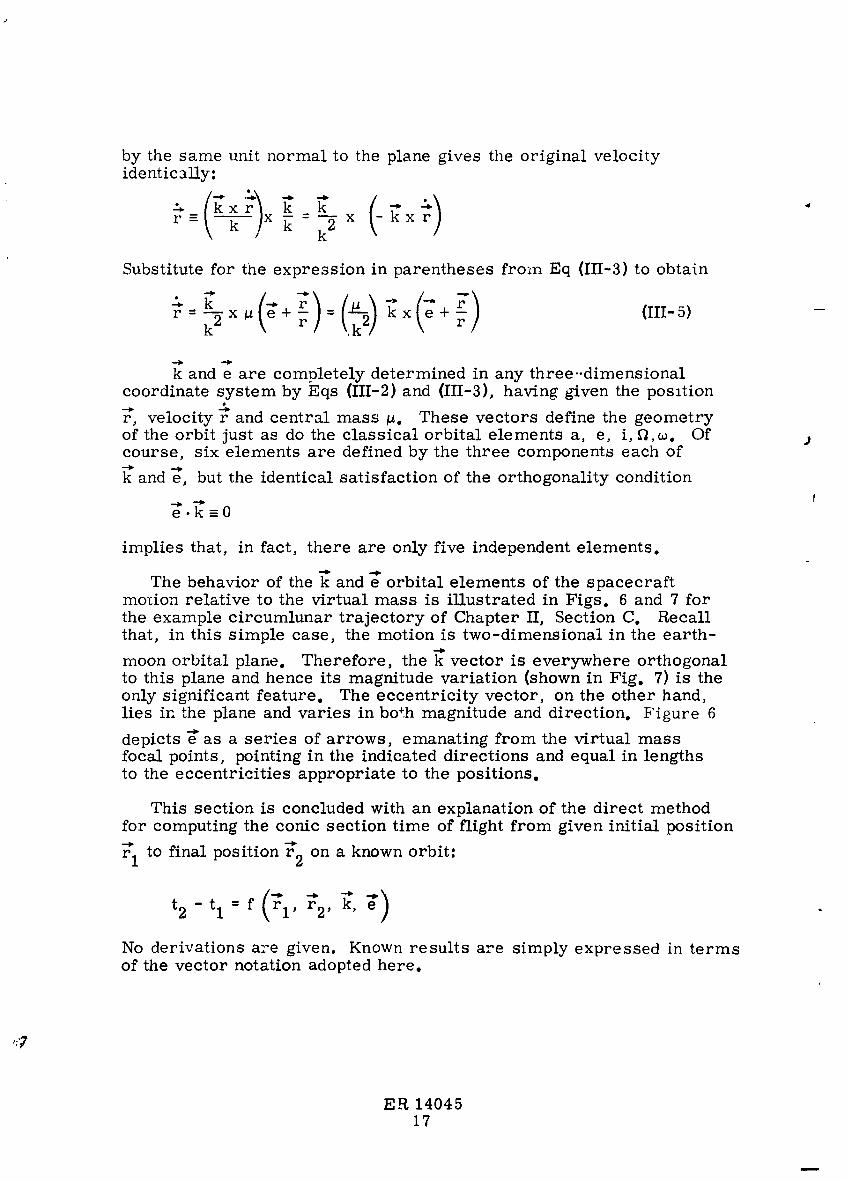
by the same unit normal to the plane gives the original velocityidentically:

g ,xg: x

Substitutefor the expression in parentheses fro':nEq (Ii_-3)to obtain

k and e are completely determined in any three--dimensionalcoordinate system by Eqs (III-2)and (III-3),having given the posltion

r, velocityr and central mass _. These vectors define the geometryof the orbit just as do the classical orbital elements a, e, i, _,_. Of •course, six elements are defined by the three components each of

k and e, but the identical satisfaction of the orthogonality condition

e.k=0

implies that, in fact, there are only five independent elements.

The behavior of the k and e orbitalelements of the spacecraftmorion relativeto the virtualmass is illustratedin Figs. 6 and 7 forthe example circumlunar trajectory of Chapter II, Section C. Recallthat, in this simple case, the motion is two-dimensional in the earth-

moon orbitalplane. Therefore, the k vector is everywhere orthogonalto thisplane and hence itsmagnitude variation (shown in Fig. 7) is theonly significantfeature. The eccentricity vector, on the other hand,lies in the plane and varies in both magnitude and direction. Figure 6

depicts _"as a series of arrows, emanating from the virtualmassfocal points, pointingin the indicated directions and equal in lengthsto the eccentricities appropriate to the positions.

This section is concluded with an explanation of the direct methodfor computing the conic section time of flight from given initial position

r1 to final position r-*2 on a known orbit:

No derivations are given, Known results are simply expressed in termsof the vector notation adopted here,

ER 1404517

1966009743-024

• e = 1. 609

220 -

69.3

200_Virtual mass

trajectory

130 60

160 e = 64.099e = 2. 146

140 -

_ 55e = 26. 260

120

o

N

"_ 100

_ 80 _e = 6.329 50

60-

e -- 1. 463

4020

35

3O

0e= 0.874

e = O. 976I I- i

-20 0 20

X I (ru_ut mix 103 )

Fig. 6. Eccentricity Vector for Various Virtual Mass Positionsfor In-Plane Trajectory

ER 1404518

I

1966009743-025

ER 1404519

1966009743-026

Section C of this Chapter describes how to handle the inverse

problem of finding the final position r on a given orbit, with a pre-2

scribed flight time from an initial position rl:

t2The conic section time of flight can be computed from

iVI2 _ M 1(III-6)

t 2 - t I = oaM

In this expression, when the orbit is elliptic or hyperbolic (e # I).

M is interpreted as the mean anomaly and ¢oM as the mean angular rate.

For the parabolic case (e = i), M is taken to be the area swept out by

the radius vector as it rotates from periapsis and ¢oM the (constant)areal rate. The value M can be represented in the algebraic form

M. = E. -@. (i= 1, 2) (III-7)1 1 1

in all cases, When e # 1, E represents the eccentric anomaly and@ = e sinE or e sinh E. In the hyperbolic case the sign of Mshouldbe reversed; but, as will be shown later, this can be accommodated in

the sign of,.M. When e = 1, E represents the area obtained by pro-

jection of the parabolic arc normal to the major axis and %5defines thetriangular area obtained by similar projection of the radius vector tothe position defining the end of the arc. The parabolic triangular areais signed negatively when the true anomaly is less than 90 ° so thatEq (IH-7) is always valid.

It remains now to show how the values of E, %b, and ¢0M are computedfor the various cases.

First, some preliminary computations are defined. The in-planeunit normal to the major axis is

-* kx e (_,# 0)n = ke

-" -- (III-8)-. kx r1

n = k r 1 (_= 0)

ER 1404520

1966009743-027

/"

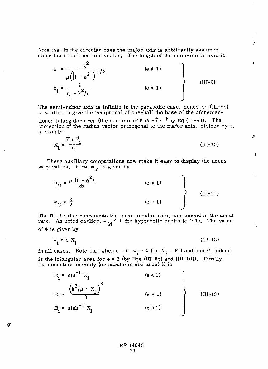
Note _hat in the circular case the major axis is arbitrarily assumedalong the initial position vector. The length of the semi-minor axis is

k 2b : (e# i)

(m-9)2 (e= i)

bi= r. - k2/u1

The semi-minor axis is infinite in the parabolic case, hence Eq (III-9b)is written to give the reciprocal of one-half the base of the aforemen-

tioned trian_ular area (the denominator is -_'. _'by Eq (III-4)). Thep:_ojection of the radius vector orthogonal to the major axis, divided by b,is simply

n.r.X. = } (III-10)l b.

1I

These auxiliary computations now make it easy to display the neces-

sary values. First ¢oM is given by°

A_(I - e2_, (e # i)f ,,-

;M kb

(III-ii)

k (e= I)=.2

The first value represents the mean angular rate, the second is the areal< 0 for hyperbolic orbits (e > 1). The valuerate. As noted earlier, tOM

of q, is given by

@i = e Xi (III-12)

in all cases. Note that whene = 0, _i = 0 (or Mi = E i) and that _iindeed

is the triangular area for e = 1 (by Eqs (III-9b) and (III-10)). Finally,the eccentric anomaly (or parabolic arc area) E is

E i = sin-I X i (e<l)

(k2/_ • X.) 3E. = i (e = 1) (Ill-13)i 3

E i = sinh'l Xi (e >I)

ER 1404521

1966009743-028

There is no ambiguity in the hyperbolic case since the orbit isaperiodic. This is reflected in the fact that the inverse hyperbolicsine is a monotonically increasing function of the argument. The am-biguity which does exist in the periodic elliptic case can be easily re-solved. When e # 0

E.1 = principal value = PV for r.1_< a

E. - _- PV for X. > 0, r. > a I (Ill-14)

1 1 1

E. = -Tr - PV for X. < 0, r. > a1 1 1

Whene = 0, the above test onr - a must be replaced by atest on

r I • r 2.

Note that the time can be negative in the case where e < 1 and the

cut E = _ (or -9) is crossed. If this should happen merely add 2_/_ M

to the time given by Eq (III-6).

B. NONITEt _&TED VERSUS ITERATED COMPUTATION

The characterization of the virtual mass motion as a constant-

velocity straight line and of the mass magnitude as held constant overeach computing interval is dynamically consistent with the characteri-zation of the spacecraft relative motion as a conic section. Therefore,an important problem concerning the computation is the determinationof a method for establishing appropriate values of the virtual mass ve-locity and mass to hold constant over the interval.

The simplest approach, of course, is to merely take the values givenby the virtual mass equations themselves at the beginning of the s_ep.These values can be used, much as in the classical Euler integrationscheme, to propagate the motion to the end of the interval, where newvalues are discontinuously assumed consistent with the new situation.This procedure is fast since just one computation (no iteration) is re-quired per time interval. Unfortunately, accuracy suffers due to thefact that initial values, rather than mean values, are used over the step.Whereas the spacecraft trajectory itself would be continuous in this case,perhaps the most serious failing would result from the discontinuitiesin the virtual mass trajectory. The virtual mass position propagated tothe end of an interval, for the purpose of locating the spacecraft, wouldnot, in general, correspond to the position computed by Eq (II-3) forthe start of the next interval.

ER 1404522

1966009743-029

/

Ifthe correct position and magnitude of the virtual mass at the endof the intervalwere known a priori, there would be no problem what-ever in establishingthe required average velocity or in choosing somelinearlyi_terpolatedvalue of the mass to hold constant: _'

r - r

__ ve vBr =v Atav

_Vav= Cl _Ve+ (1 - C 1)_vB (0 _<C 1_< 1is a specified constant)

(III-15)

Since these finalvalues are not known at the outset, but are in fact partof the answer sought, an iterativecomputation procedure, analogousto the modified Euler scheme, is suggested. The finalvalues r_ and

V 2e

_v are estimated initiallyand then iterativelyimproved by computatione

based upon the resultingspacecraft finalposition. When the differencebetween successive values becomes acceptably small, the iterationcanbe discontinued and the computation can proceed to the next interval.The better the initialestimate, naturally, the faster the convergence.The method decided upon for study was to assume a second order varia-tion with time in computing this firstguess.

r = rvB + v_B (At)+ r (At)2

I

V e Vav

_ve : _vB + _vB (At)+ _Vav (At)2 (III-16)

The constant terms are given by Eqs (II-3),the linear term coefficientsby Eqs (II-4). The (acceleration)coefficientsof the squared terms areassumed to hold for this interval from the previous one. Thus, theywould be computed as

r - r - r (_t)•. V V V-_ e B Br =

Vav (At)2(III-17)

Uve - _v B - _v B (At)oo

DV =av (At)2

,7

ER 14045

23

I

1966009743-030

afLer convergence was achieved in the preceding in rval. At the start-ing time step, they are set to 0. Although this iterative scheme isslightly more complicated and requires multiple looping each interval,there will be no discontinuity in the virtual mass trajectory, and accu-racy should be better, for a given step size, than with the simple non-iterative approach.

C. THE COMPUTING INTERVAL

It is intuitively obvious that different computing interval sizes arerequired for different l_arts of a trajectory. Large step sizes can beused when the spacecraft is far away from a relatively constant magni-tude and slowly moving virtual mass (such as would be the case duringthe heliocentric arc of an interplanetary mission). Small incrementsshould be taken, however, whenever the vehicle is close to the virtualmass (as for a trajectory grazing by a planet) or whenever a sphere-of-influence crossing occurs and the virtual mass moves and changesmagnitude rapidly from one dominant physical body to another.

If the step size is controlled to maintain equal increments of trueanomaly in the motion relative to the virtual mass, the time incrementvariation will behave qualitatively as desired. The simple formula forconverting the true anomaly increment into the corresponding time in-terval is

2C 2 rvs

At : k (111-18)

where k is the magnitude of k and where C2 is an input constant defining2

the desired angular step size in radians. Multiplication of C 2 by rvs ,

of course, converts the angle into twice the area increment. Dividingby double the instantaneous areal rate relative to the virtual mass gives(for small steps) the time to cover this angle.

A practical difficulty could arise in attempting to use Eq (III-18) asit is. Figure 7 shows that k vanishes at one point along the trajectoryfor the in-plane case. At this point, of course, the relative motion isdirectly toward or away from the virtual mass. Although k does notvanish for more general trajectories, it still can become small enoughto cause Eq (III-18) to compute a very large time increment. This

problem can be circumvented by replacing k by rvs Vvs, the scalar

product of the position and velocity magnitudes. This then representsa fictitious areal rate which assumes that the velocity is always normalto the position vector and thus, in general, is larger than the true arealrate. Substituting this into Eq (III-18) gives

ER 1404524

1966009743-031

/

C 2 rvs (III-19)At= V

vS"4

as the time increment. This form can give computational difficulty

only when Vvs _ 0--a highly unlikely occurrence.

it is one thing to set the desired time increment, but the realizationof it is another matter. Since the conic section time of flight is a trans-cendental form, it is not possible to invert it to determine in closedform the final position corresponding to a given flight time from agiven initial position. Two alternatives are possible, depending uponwhether the basic computation philosophy is noniterative or iterative(see Section B). In the noniterative approach, the final position is es-timated so as to approximate the desired time. Once the estimate ismade, the desired time is disregarded and the conic section time offlight equations are used to ascertain what time ac aally did elapse j

from r1 to the estimated _'2" The trajectory time and ephemeris timeare then updated by this true time increment in preparation for the rnext step.

The iterative procedure cannot be treated so simply, however, be-cause the procedures for estimating and updating the final values of the -virtual mass and for computing the average velocity all depend uponacbieving a predetermined time increment with very high accuracy.A double iteration could be mechanized in which the spacecraft finalposition is iterated within the outer loop of the virtual mass final con-dition iteration. Such a procedure is cumbersome and time-consuming.It is also unnecessary if accurate initial estimates of both the space-craft and tlae virtual mass final conditions can be made and then simul-taneously updated within a single iteration loop. This latter course wasdecided upon for the mechanization of the iterated virtual mass proce-dure. The logical details of the technique are not of primary concernhere and, hence, are deferred until Chapters V and VI. The establish-ment of the computation interval is the subject of interest here.

It has been shown that an accurate estimation procedure for thespacecraft final relative position is required for both the noniterativeand the iterative approaches. Since this estimate, itself, will be re-peatedly applied in the iterative scheme, the objective is to develop anestimation procedure which improves with each iteration.

The spacecraft and virtual mass data are known at the beginning ofthe interval. The virtual mass magnitude and velocity are given by Eqs(II-3) and (II-4) for the noniterated case or by Eqs (III-1 5) for the iteratedcase. The initial relative position and velocity and the mass, therefore,

ER 1404525

1966009743-032

Z

are triviallydetecrnined and from them, the vector orbitalelements

_, e are obtained by Eqs (III-2)and (III-3).Equation (Ill-19)gives thedesired step size,At. The finalposition F' must lie in the plane of

vs2

relative motion defined by rvs 1, rvsI and, hence, can be expressed asa linear combination of them:

+ (Z_r) - Bavs 2 (III-20)rvs2 = B Sl Sl

The geometry is illustratedin Fig. 8 and shows that Avdetermines thetime (or true anomaly) increment and B ensures satisfactionof the orbitalequation. Once A_ is given, B is easily computed since Eq (_I-20) mustsatisfyEq (III-4):

k2/UvU : (III-21 )

e.o +ovs2 vs2

The question therefore is reduced to that of relating A 7 to the de-sired At. As in the case of the virtual mass estimation procedure, asecond order variation will be assumed. Here the constant term is 0and the linear coefficient is 1, for it must be true that A7 -_ At as At -_ 0

AT =_ t + _ (_t) 2 (III-22)

The procedure for evaluating K is similar to that used for the secondorder coefficients in Eq (III-16). After the computation of the conic

section time of flight At k = t 2 - t I (from Eq (III-6)) in the preceding

iteration, that A t k value and the A 7 value used to obtain it specify theexact _ for that case as

AT- At k" 2 (III-23)

This value will be assumed to hold for the present iteration from the

last one. Clearly, this assumption gets better and better as & t k-* & t,

the desired time increment° In the noniterated ease _ is merely updatedto provide the best first (and only) estimate of the next interval.

ER 1404526

q r

1966009743-033

'l

The study reported in Ref. 2 showed that, under some circumstances,the conic section time of flight m_v be different from the true time. Inthe event sucb a time bias night prove desirable in this case, the pro-

vision was m_de to causeAt k -* C 3 At by rewriting Eq (III-22) as

A,r = C 3At+ _ [C 3 _t]2 (III-24)

where C 3 is an input constant.

--_ ra _ vs 1 J

Conic Section vs 2Orbit

[

(Ar)_vs 1

Fig. 8. Geomet_ of Spacecraft Final _elatlve Position Determination

2

ER 1404527

I I

1966009743-034

ER 14045

28

1966009743-035

/

IV. DIGITAL COMPUTER STUDY

A. APPROACH,41

The suitabii._ty of the virtual mass technique as a flexible integrationmethod for the n-body problem could be assessed only by trying somenumerical examples. Accordingly, the basic concept described in Chap-ter II was mechanized, in conformity with the considerations of ChapterIll, as two separate computer programs: one a simple noniterative pro-cedure, the other a somewhat more complicated iterative procedure.Salient features of the flow diagrams for the two programs are sketchedin Fig. 9. Details such as special logic paths for starting the computa-tion and tests for stopping conditions and printout have been omitted inorder to emphasize the basic principles of operation. Reference ismade on the flow diagrams to the sections of the two previous chapterswhere the appropriate equations may be found. Note that the iteratedprogram loops through the ephemeris subroutine only once each compu-tation interval. Since the desired time increment At is fixed and theiteration procedure is intended to make repetitive improvement to achievethis objective, the final time and, hence, the gravitating body data arefixed. Improvement in the virtual mass data, therefore, is effected by timprovement in the spacecraft final position and velocity.

The input constants provide the means by which the computations are -

controlled within the programs. C 2 sets the desired computation inter-

val size (see Section III-C). C 3 biases the Keplerian flight time for valuesdifferent from unity (see Section III-C). In the iterated program C 1

(0 < C 1 < i) linearly interpolates the virtual mass magnitude to somevalue between the initial and final values (see Section III-B). The con-stant LOOP controls the number of iterations per computing intervalaccording to the following:

Value of LOOP No. of iterations (afterfirstpass)

12 16 24 33 42 61 12

In order to properly assess the effectsof variations of the programcontrols and to compare the two programs with each other, an indexto the accuracy of the solutionis necessary. The constancy of the Jacobiintegral is a necessary condition to any solution to the restricted three-body problem and, therefore, could be used for just such an accuracy index.

f

ER 1404529

!

1966009743-036

In addition, this case of just two gravitating bodies is the simplest n-body problem and would serve adequately as a test of the integrationmethod. Therefore, the ephemeris subroutine was programmed forthe restricted three-body problem by representing two bodies in circu-lar orbits about their common center of mass. The expression for theJacobi integral is classically derived in the rotating barycentric coor-dinate system. Since all computations for the virtual mass procedureare carried out in an inertially oriented barycentric frame, the Jacobiconstant was transformed to that reference:

cj = 2 + - ( s)2 - (Ys - - (Ys - x )rls r2s s

It was recognized that some of the computations represented by theequations in Chapters II and III may involve differences between nearlyequal numbers. Loss of significance in such cases can be alleviated bycarrying out these computations in double precision. Rather than at-tempt an analysis in detail to isolate those computations where increasedaccuracy would be required, all computations were done in double pre-cision on the IBM 7094 digital computer.

A circumlunar trajectory, inclined initially nearly 30 ° to the earth-moon plane, was chosen as the principal test trajectory. The pericyn-thion altitude of about 210 naut mi (lunar radius --938.5 naut mi) wasreached in slightly more than 70.3 hr from insertion at earth. Thistrajectory is given in Chapter V as a sample problem solved by thefinal version of the program, All the details, including the initial con-ditions, the physical constants describing the earth-moon system andthe trajectory time-history, appear there.

B. RESULTS

Although a great number of exploratory studies and parametric runshad to be made, the pertinent results can be summarized quite concisely.

As expected, the iterated program was more accurate than the simplenoniterated one. A direct comparison of the two is shown _n Fig. 10 interms of the Jacobi energy accuracy index. The gains controlling the

computing interval size, C 2 = 0. 0005, and the time bias, C 3, wereset to the same values for the two programs. The curve shows thedifference between the Jacobi energies at corresponding time pointson the test trajectory as computed by the two programs. This methodof presentation was chosen because, although the gains selected causedthe iterated program to compute with high accuracy, there was a smallvariation of the Jacobi energy. The difference shown in the curve ofFig. 10 shows how much worse the variation was using the noniterative

ER 1404530

l

1966009743-037

ER 14045

31

1966009743-038

program. The maximum difference was an appreciable 9000 (naut mi/

hr) 2 out of 7033989. 7388 (nautmi/hr) 2. As will become more apparentin the other studies of the iterative program, the superior performanceof the more sophisticated method well justifies the slight additionalcomplication. Without it, the calculation of precision trajectorieswould be impractical.

Restrict±.lg attention, therefore, to the ._terative program, the firstquestion to be resolved was that of the number of iterations required

per computing interval. With any reasonable gain C 2 on the computinginterval size, it was found that just one extra loop (after the first pass)was sufficient to produce answers which, io at least eight significantfigures, were identical with those for more repetitions. Therefore, thefinal program has been fixed to loop the first time through the computa-tions, including an access to the ephemeris subroutine, and then justone additional iteration (by-passing the ephemeris).

The studies of the interpolated virtual mass value and the conic sec-tion time bias are summarized in Figs. 11 and 12. For both of thesecomparisons, a base run was made with the mass interpolated at the

midpoint (C 1 = 0.5) and no time bias (C 3 = 1.0). The curve of Fig. 11

was generated as the _ime-history of the differences in the Jacobi

energy between the base run and two others in which C 1 = 0.4 and 0.6.

The incremental error buildup portrayed by this graph clearly showsthat the best mass value to use is the arithmetic mean between the initialand final values. Similarly, the incremental error curve of Fig. 12 was

generated as deviations from the base run of two time biases of C 3 =0. 99999 and 1. 00001. This curve shows the extreme sensitivity of the

solution accuracy to this parameter and indicates that no bias (C 3 = 1.0)is best. On the basis of these results, the final version of the programis coded to calculate the virtual mass magnitude as the simple averageof the end-values and to achieve an unbiased match between the desiredand the conic section time increments.

The constant C2, since it controls the computation interval size, isthe basic accuracy selector. Final comparative studies of this param-eter were made with the other program controls set to the optimizedvalues as described above. The variation of the Jacobi energy with time

along the test trajectory is shown in Fig. 13 for various gains C 2. A

value of C 2 <__0.001 maintains the maximum deviation to less than 2 (nautmi/hr) 2 out of the 7033989.7388 (naut mi/hr) 2 initial value. The discon-tinuity in the curves at approximately 38.9 hr is due to a computationalinaccuracy which occurs as a result of the fact that the computing inter-val spans the apocenter relative to the virtual mass. As noted, the dis-cussion of the time of flight in Chapter III Section A, such an occurrence

ER 1404532

1966009743-039

I I i I oCD CD CD O CDCD _ CD CDC_ CD O 0

I="4

ER 1404533

1966009743-040

8O

60

<3

_ 40

.p.,f

• 20

00

0_0

10 20 _

30 _ 40 50 60Trajectory Time, t (hr) 70

Fig. 12. Variationof JacoblEnergyDue to Time Blas oflaC31 --o.oo001 (CO.= 7033989.7)

ER 1404534

1966009743-041

ER 14045

1966009743-042

would cause the formulas to compute a large negative value for the timeof flight. The program was provided with the capability to theoreticallycorrect this mistaku by adding a time equal to one period of the orbit.Unfortunately, some loss of significance occurs due to the subtractionof two nearly equal numbers. Apparently, the resulting inaccuracy isenough to cause the Jacobi energy variation indicated. This difficultyshould be less serious for a macaine such as the CDC 3600 than as shownhere for the IBM 7094. The former carries 20 digits in double precisionand also has automatic rounding, whereas the latter carries only 16 digitsand simply truncates.

To gain some insight into what these variations in the Jacobi energymean in terms of the spacecraft positional deviations, the difference_ _r

were computed between the base run with C 2 = 0. 001 and other trajec-

tories run with gain_ C 2 > 0. 001. These differences, divided by the

magnitude of the spacecraft position vector from the barycenter, areshown plotted in Fig. 14. They show, as an example, that a gain ofC 2 = 0. 005 gives a positional displacement of &r = 0. 307 naut mi for

a total position vector distance of r = 197299.51 naut mi at 65.0 hr(just prior to the pericynthion at 70. 338787 hr). Figure 13 shows that

this same trajectory showed a Jacobi energy variation of &Cj = 44.66(naut mi/hr) 2 at this time.

An independent check of this Jacobi energy versus position deviationcorrespondence was made by comparing the same base run with identicallythe same trajectory numerically integrated by a standard procedure in anentirely different computer program. The integration tolerance happenedto be set in that program so that the resulting solution displayed a Jacobienergy variation at 65 hr which was very nearly the same as that noted

above (for the C 2 = 0.005 case). The positional difference between the

numerically integrated trajectory and the base run was also approximatelythe same _r = 0.384 naut mi. Thus, it is concluded that the Jacobi energydoes provide a good index to accuracy and that the base run apparently isa_, accurate solution to the problem.

Of course, the price of accuracy is computation time. The run with

gain C 2 = 0.005 calculated the trajectory in 2369 increments and took 57

sec on the computer. This time was measured for a complete problemcycle, from the time the instruction was given to read the input datauntil the program again sought data for the next problem.

Program accuracy control by means of the constant C 2 would requiresome study on the part of the user to determine what value to use to ob-tain a certain accuracy and to estimate th_ expected running time on thecomputer. The problem has been simplified somewhat by utilizing some

ER 1404536

1966009743-043

-510

/

-II

10 -6 .

J

_ f

10 -7

m

m

10 8 : I I, , I J0 10 30 30 40 50 60 70

Trajectory Time (hr)

Fig. i_. Sl_.cecraftPositionVector Error as a Functionof Time for Various ComputingStepISi:_eGains, C2

ER 1404537

t

1966009743-044

information obtained from a cross-plot of Fig. 14. Since the maximum

error occurs at the 70-hv point near pericynthion, a plot of C 2 versus

Ar/r at 70 hr was made as shown in Fig. 15. This curve was approxi-mated by a second degree polynomial fit and built into the initializationsection of the program. Thus, the user can input the more intuitivelymeaningful number At/r, or fractional accuracy desired at pericynthion,and the program will internally set its own gain appropriately.

1966009743-045

Y

-i0

-8

-6[}

_ ,

-4

-2

O, i , jO -5 -I0 -15 -20 -25

loge (At/r)t = 70 (hr) i._

Fig. 15. Correlation of Computing Interval Gain C2 withPosition Error at t = 70 (hr)

ER 14045

39

1966009743-046

BLANK PAGE

1966009743-047

! ,

, /

" V. GENERAL DESCRIPTION AND USE OF THE VIRTUAL

( MASS PROGRAM FOR COMPUTING SPACE TRAJECTORIES• "i_ 4

This chapter is intended to serve two purposes.

._ (1) It can be used, independently of the rest of this report, by::_ the mission analyst. Usually he is not so much concerned:i

, _ about the computation process or the implementation of the':: procedure. Instead he is more interested in what general:;• problem is solved, what is the solution accuracy and how_ can he use this digital computer program to calculatet:'_.•_.,, trajectories.f ;A

_ (,_:_ (2) It also provides a broad overview of the digital program and_,;,# its use, uncluttered by details. Thus it serves as an intro-

duction to the trajectory analyst who may be interested inthe details given in Chapter VI.

A. GENERAL DESCRIPTION

The purpose of this contract was to investigate the feasibility ofthe technique of computing space trajectories as a series of conicsection solutions relative to a moving and varying virtual mass. At "every instant of time this virtual mass replaces the combined effectsof all the gravitating bodies upon the spacecraft. As explained in the

_ preceding chapter, this was done by testing the procedure in a digitalcomputer program. The simplest n-body problem, the restricted

_ three-body problem, was used for this purpose. The final version ofthis FORTRAN IV source program is delivered with this report infulfillment of the obligations under the contract.

Although this program solves only the restricted three-bodyproblem, the virtual mass subroutine was formulated in completelygeneral form. Thus, the only changes required in the program tomake it capable of computing trajectories for more than two gravitat-ing bodies are to replace the ephemeris and the input and output sub-routines.

The reference coordinate system is a set of inertially oriented

axes, centered at the barycenter. The xy plane is the earth-moonorbital plane and the initial position of the moon (and hence the earth)

is given in terms of the ephemeris time tep h, or time since the moon!__ crossed the positive x-axis. Specification of the earth-moon distance_, D, the angular rate _ and the ratio of moon mass to total system mass

complete the description of the gravitational environment. The total

m

ER 1404541

1966009743-048

mass of the system (times the Universal Gravitation Constant) is com-puted internallyin the program as

2 D3 (V- I)AUe+ _m = _

to ensure dynamical consistency of the system. The spacecraft initialposition and velocity components are specified in the reference bary-centric coordinate system.

To permit the greatest freedom possible in the use of the programand to scale numbers for greatest computational accuracy, all calcula-tions within the program are carried out using d_mensionless quantities.Thus, no units are specified (except that_ is presumed given in degreesper unit time) and the user may input tilenecessary data in any system

-1 .

of units he chooses. The value of _ Is chosen as the unit of time and

D as the unit of length. Thus, conversion factors

_-I = time

D = length

D = velocity

2 D 3 = mass times Universal Gravitation Constant

3 D 3 : mass rate

etc.

are used to nondimensionalize input data and to convert din,ensionlesscomputed values to output data in the same system of units as the in-put.

The program has been discussed here in terms of the earth-moonsystem but, of course, is applicable to any two bodies (e.g., sun anda planet). The input constants determine the detailsof the system.Itis only necessary to remember that the ephemeris time gives thetime elapsed since the body designated by mass ratio _ (0< # < i)crossed the x-axis.

As described in Chapte:- IV, Section B, the accuracy of the solu-tionis controlled by an input number Ar/r. This quantity representsthe allowable error (nondimensionalized by D) in spacecraft positionat the pericynthion point for an earth-moon trajectory. The programautomatically converts thisnumber to an equivalent gain controllingthe computing interval size to maintain roughly equal steps in trueanomaly relative to the virtual mass (see Chapter III,Section C).The gain correspondence was established for the lunar trajectory anditis not known at present what performance could be expected for an

ER 1404542

r

1966009743-049

interplanetary trajectory (i, e., one which does not pass close to thelarge body).

The computing interval is adjusted as a print time is approachedto cause the printout to occur exactly at a specified time increment.A similar adjustment is made whenever a major axis (pericenter orap'_center) crossing is imminent. The simp;e logic for this latteradjustment is not adequate for all cases. The pericenter crossingsare picked up rather consistently except when such a crossing occursshortly after the initial point (this is tl • case for the test trajectoryselected) and a very loose gain is used. In this situation the programsteps over this region before it has a chance to anticipate it. Theapocenter crossing (which occurs at about 38.9 hr for the test traject-ory) is only rarely caught by the routine provided.

Three stopping conditions are specified as input data, and theproblem will terminate on whichever condition is met first. The con-ditions are a maximum allowable trajectory time and an impact witheither of the two gravitating bodies. The radii of the two bodies mustbe given.

B. INPUT AND OUTPUT .

A series of from 2 to 7 cards (I to 6 data cards and 1 problemcard) is used to input the data for a given problem. A number ofproblems may be run consecutively by ,nputting a sequence of suchseries of cards. Formats for the 7 cards are given below. The con-trol word on each card begins in Column 1 and must appear exactlyas specified. The variables begin in the columns indicated and mustbe punched according to the standard FORTRAN formats supplied(D18.0 indicates a double precision numeric field of 18 columns andI 1 indicates an integer field of 1 column).

Data Card l--

Col. i Col. 9(Dl8.0) Col. 27(D18.0) Col. 45(D18.0) Col. 63(D18.0)

POSITION t xs Ys Zs

Data Card 2--

Col. 1 Col. 9(D18.0) Col. 27(D18.0) Col. 45(D18.0)

VELOCITY _s _'s Zs

ER 1404543

'_ H 'i

1966009743-050

Data Card 3--

Col. l Coi. 9(D18.0) Coi. 27(D18.0) Coi. 45(D18.0) Coi. 63(D18.0)

EFEMERIS teph _ D

Data Card 4--

Col. 1 Col. 9 (DI8.0)

ACCURACY _.r/r

Data Card 5--

Col. i Col. 9(DlS. 0) Col. 27(D18.0) Col. 45(D18.0)

STOP tf rls F r2s F

Data Card 6--

Col. 1 Coi. 9(D18.0) Coi.42(II) Coi. 43(Ii) Coi. 44(Ii)

PRINT At IPRT I IPRT2 IPRT3P

IPRT1, IPRT2, and IPRT3 are used to indicate printout option requests..Ordinarily (and in case Columns 42 to 44 of this card are left blank),only the standard block of printout is given (see discussion below onoutput). However, any or all of the optional printout blocks may beobtained at each print interval by using the integers 1, 2, and 3 inColumns 42 to 44. A 1 appearing anywhere in these columns wouldrequest the first optional block in addition to the standard block ofoutput. A 2 would request the second optional block, and a 3, thethird. Thus, any combination of the integers 1, 2, and 3 may appearin any of the three columns to request any combination of the 3 optionalblocks in addition to the standard block.

Problem Card--

Col. 1 Col. 9 (D18.0)

PROBLEM NPROB

NPROB is the problem number and will be truncated to an integerbefore being stored by the program. This number in used to identifythe output.

ER 140_544

1966009743-051

t

To make the program as convenient to use as possible, certainflexibilities of the input have been incorporated in the program:

(1) For a_y problem, the six data cards may appear in any 'order. The problem card, however, must always appearlast.

(2) On the first problem of a job, the data cards PRINT andACCURACY may be omitted. If the PRINT card is omitted,

A¥ is assumed to be 5., and only the standard block of out-put is given. If the ACCURACY card is omitted, Ar/r isassumed to be 1. D-7.

(3) On any problem after the first problem of a job, any of the6 data cards may be omitted. For those cards which donot appear in a given problem, the variables used in thefirst problem are always assumed. The problem card can -"never be omitted and must always be the last input card fora problem.

!

(4) Any of the variable fields, if left blank, are assumed to be0. DO.

For each problem, the input data are printed out as the first pageof output. The sequence of fields corresponds to those on the inputcards, but the cards are ordered in a standard sequence and anyassumed cards (by omission assumed same as first problem) are alsoprinted.

Subsequent pages of output for each problem give the standard blockof output, follo_ved by any optional blocks requested, at each printinginterval. The optional blocks are always ordered 1, 2, and 3 if theyappear. (See the PRINT data card for the method of requesting op-tional blocks of output. ) All variables are dimensioned in the sameunits an the input.

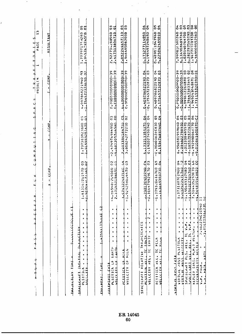
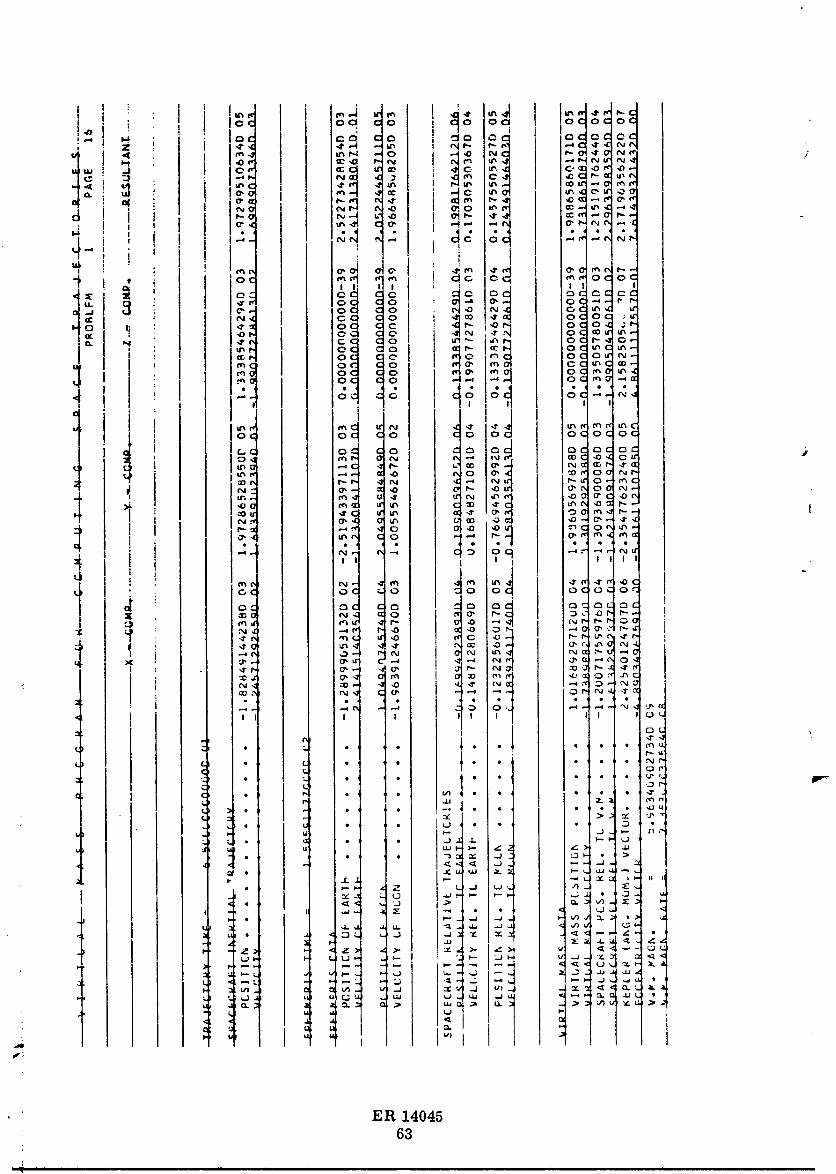
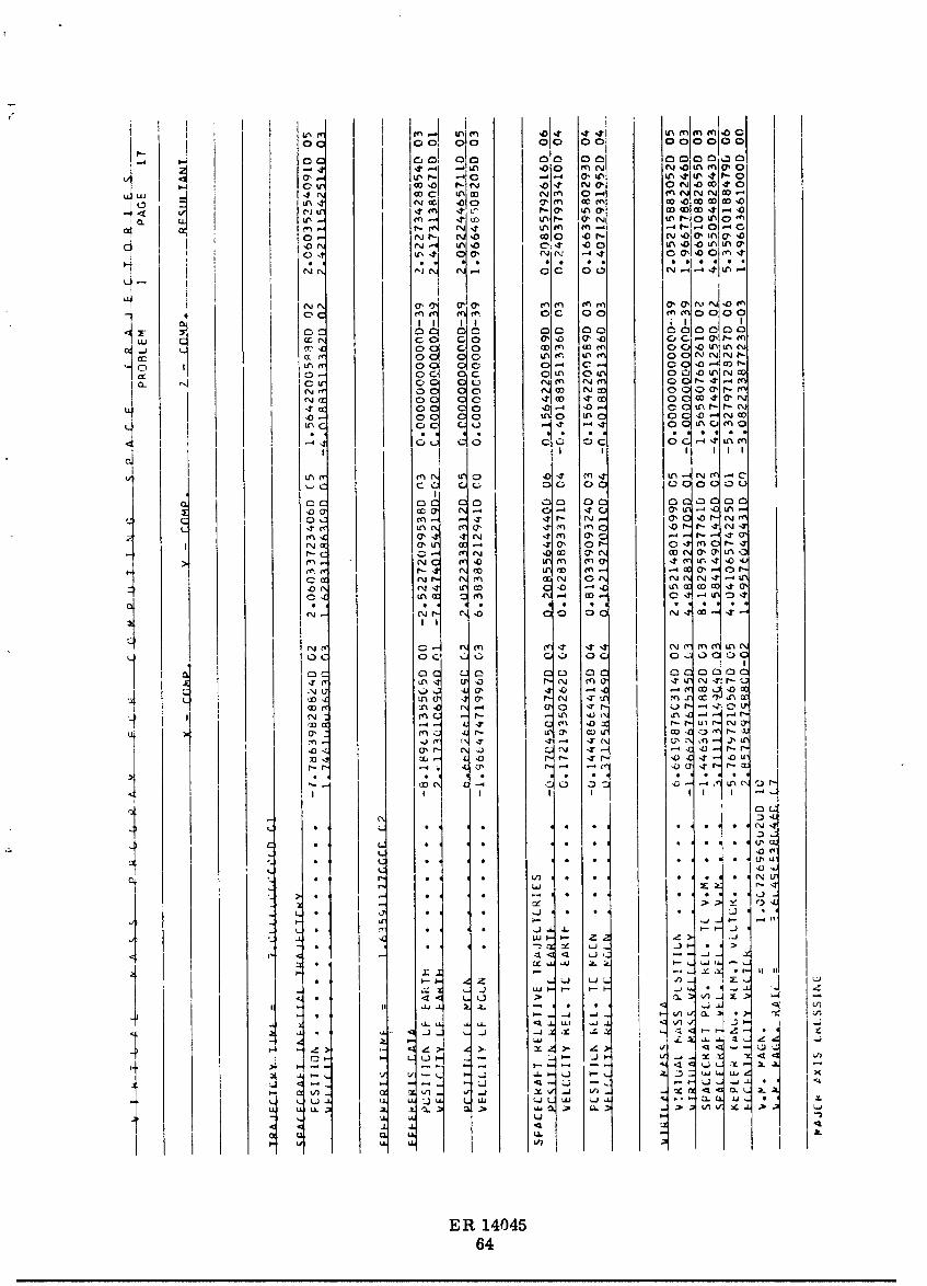
Standard output block (option 0)

TRAJECTORY TIME = t

SPACECRAFT INERTIAL TRAJECTORY

POSITION ..... x s Ys Zs rs

VELOCITY .... Xs Ys Zs rs

Optional output block 1

EPHEMERIS TIME = tep h

ER 1404545

1966009743-052

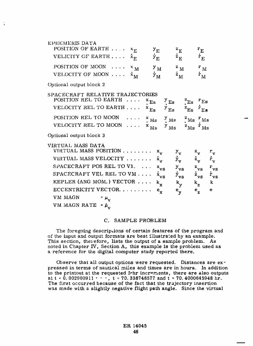
EPttEMERIS DATA

POSITION OF EARTH .... x E YE ZE rE

VELICITY OF EARTH .... _E YE iN _E

POSITION OF MOON .... x M Y M z M r M

VELOCITY OF MOON .... :_M YM _M )M

Optional output block 2

SPACECRAFT RELATIVE TRAJECTORIESz

POSITION REL TO EARTH .... XEs YEs .Es rEs

VELOCITY REL TO EARTH .... XEs YEs ZEs _'Es

POSITION REL TO MOON .... x. Ms Y.Ms ZMs rMs

VELOCITY REL TO MOON .... XMs Y Ms ZMs rMs

Optional output block 3

VIRTUAL MASS DATA

VIRTUAL MASS POSITION ........ x v Yv Zv rv

VIRTUAL MASS VELOCITY ....... _v Yv _v _v

SPACECRAFT POS REL TO VI_.... Xvs Yvs Zvs rvs

SPACECRAFT VEL REL TO VM .... Xvs Yvs Zvs l"vsKEPLER (ANG MOM. ) VECTOR .... k k k k

x y zECCENTRICITY VECTOR ......... e e e e

x y z

VM MAGN = /_v

VM MAGN RATE = _v

C. SAMPLE PROBLEM

The foregoing descrip,ions of certain features of the program andof the input and output formats are best illustrated by an example.This section, therefore, lists the output of a sample problem. Asnoted in Chapter IV, Section A, this example is the problem used asa reference for the digital computer study reported there.

Observe that all output options were requested. Distances are ex-pressed in terms of nautical miles and times are in hours. In additionto the printout at the requested 5-hr increments, there are also outputsat t = 0.002900911 • • ", t = 70. 338748577 and t = 70. 4000645948 hr.The first o,.curred-" because of the fact that the trajectory insertionwas made with a slightly negative flight path angle. Since the virtual

ER 1404546

m

1966009743-053

mass almost exactly coincides with the location of the earth, periapsisrelative to the fictitiousbody was achieved almost immediately. Thesecond time corresponds to the periapsis passage at pericynthion.Both of these occurrences were preceded by the notation "MAJOIt AXISCROSSING" in tile printout. The last time point was printed as one ofthe stopping conditions (maximum time t = 70.4 hr) was met.

For the ACCURACY used in this example, the Jacobi energy varia-

tion was less than 2 parts out of Cj = 7033989.7 (naut mi/hr) 2.

J

m

I

ER 1404547

1966009743-054

C. 0I

00 0

< 0 g"I_

v (7' 4"

2

OC _J 0

_E r_ Q

(,_C 0 C..:)C 0 '3

or_ tx r_

I

!

_ ur, ..-_ _J,Dml_ 4"

__'_.i_

I

II

I

ER 1404548

m

[]

1966009743-055

ER 1404549

u

1966009743-056

ER 14045 [5O

im .....

g_OOg743-057

ER 1404551

1966009743-058

ER 1404552

ii inn I n r n_m

1966009743-059

ocl oc c o cJo o¢ oc ocloco I

i_ _ oc c _2 _o c) c oc _c]locv mot m_ - o Nr 4 N. _or_ =0c f e, o nr m, c-_, oI.IL ILU J ,-al_l abe U' _O _ .-4_ e_ _CIIN_ ;

.al vii ,tq <lff ,t u_ ..-o *_ O_,tC I*-(_ r_¢l.-*_O u_ O't *'q_ d _ e_l NC et_C rqr,.I,or,.

a OI .4¢ r-r_ _ <1 (3" C0,1 .-,-1 r cot- o[

-< i_ t C 0 _ r_ .*_ 00_ _JUl,0P 4

_)eq r_l_ _ Cl OC .a. mcqr 0I.,.-4

,1

I I ! I J ! I I< :IE: C:I, r,c C C_ _ C_ C:)C IC_C OCIC_C

uJ . 0_.-_ 0". I_c 0'_'1 *'_r_P.-t OC r 0,', ..J _J m_ OC C _ _lu_ _ur IOC _qClO,<l

I- 0 II *.-I OC C 0 O_ O' _'¢_ I OC NI_,O_,," O'q OC C 0 _ ,. ,0,,1 OC .,1 co--*r,

r u OC C 0 _1('_1 *q*_ OC U_rl,l -_,m_l OC C 0 0t *',_ O,_ OC tn.,_.e_ur

- O, ral OC • C ,11N ,I)_ OC O'Ol_C,o_ oc c o _,,, o,_ c¢ .o.-,®,,

I _.ur OC O" _ ,0 ,(

_. a-_i oc C (J _m

,,, ®_ de c o c_c_ oc c:c a0 Ul ,o uri Ii

o i

oc_ _c - o¢Ic_oc

,tl_ 0-'1 ,,,_ a_ <P C

2' ,.1",,1 0 U'I_ ,0 0" .-I _., .-I P- N ,..Y _'unql r--cq 41 (_ r.- I_ ,G_I oo0_oo,

I N.4 _Ot'N _" P" _Z_ l

.... a: o ..... _'_I I II I I I I

o i

' ! I

i _ I"-. ,-I _ 0 ,0

,-.,* u_ *'_ ..1 m ,-4 C) I _-,11 ,,a" c_ r,*,l.

1 < o, _ 11 _m u l o a tool r r_N _

I _ r.-_ ,_,I *"_ _1_._ (_ ,0 ,-_ (%1 lU_ _-.I t.'_ r'l t_l _(J ,0 ,:

z " " c_ ..... _<, I I I I .-4..

,Y _lr

' _ I •" 1 •..... "_"_1_t • • 4 • • ) • 0u -/ c,_u

• I " t " uJ_ ' .... :1_ :_ " o_r"4) 0, • • i • _ , • • _ • • ) c :2Jp

) e • , • ._.) J .Jt. I I- I-f_) I) U,Jl- _ _ 2 Z >I I'JJ

• • ' " ) " 'Y "1" "-11" ;P >c_ _-, • Yu u :_ _ I- __" * P n i2..[ a.--

• I- I- a _ L (J q-);. _/)- _'_-

• ,.1[< _ _.J .> :1 _ ) : I-UJ J 2; .-4 , * • _ x:

[--_ .J ..J .

L J e _C ' 'LJ ll". ,.Y. "Y'2 (. <I< I- ;'. • ,

(_CL.J_- I_.J*- _"- ,0-, L.JP, c ..I.l"_'_ C "_

. :-- (.. _ I-,. _ ,_1 u_ I- LJ t-,_. ._ "_ L_ I I_J_

;_1_ _')_ I.J _ _J _q_ . "4 O.kI(.lu o_u I ,.I.I _1 _. I I.la _lu, o _ .'_ 0

u,

ER 1404553

i i n

1966009743-060

ER 1404554

1966009743-061

ER 1404555

p i

1966009743-062

E_ 1404556

i

1966009743-063

ER 1404557

1966009743-064

ER 1404558

i 1 i

1966009743-065

ER 14045," 59

1966009743-066

ER 140456O

i i i

1966009743-067

ER 1404561

i1|1 r iiiiiiiiiii ,i.i • /

1966009743-068

ii i • i /

1966009743-069

ER 1404563

-- n i iii

1966009743-070

ER 1404564

1966009743-071

ER 14045e

65

!

1966009743-072

ER 1404566

1966009743-073

/

VI. DETAILS OF THE COMPUTER PROGRAM

The detailed derivations of all the equations have been given inChapters II and III. It is the purpose of this chapter, therefore,merely to facilitate the thorough understanding of how these equationshave been implemented in the digital computer program, the FORTRANlisting of which appears in Section C of this chapter.

A. FLOW DIAGRAMS

There are only two areas concerned with the basic computationprocedure where the logic becomes at all involved. These are theMAIN program structure itself and the time of flight calculation with-in the subroutine VECTOR. The other computational subroutines arestraightforward procedures for evaluating the equations as derived.The logic is somewhat complicated within the INPUT and PRINT sub-routines to provide the very flexible operational features described inChapter V, Section B. These subroutines, however, are not essentialto the basic computational procedure of the program and hence will not Ibe flow diagrammed here. Flow diagrams for the two sections men-tioned above (MAIN and VECTOR) are shown in Figs. 16 and 17, re-spectively, with the equations written in the algebraic notation intro-duced earlier. The numbers appearing in the left-hand margins of theblocks are external formula numbers and can be correlated directlywith the FORTRAN listing of the program in .Section C. The titlesappearing above some of the blocks correspond with the comments inthe listings.

In the MAIN program sketched in Fig. 16, the indicated subroutinesare as follows:

Subroutine De s eription .,

INPUT In conjunction with other subroutines (DINPT, SPACE(LINES), NEWPGE) and with BLOCK DATA, reads indata, performs conversions and initialization calcula-tions, and prints out the input data. Sets ITRAT = 3,KOUNT -- i.

EPHEI_I Computes the position and velocity components of twogravitating bodies (in circular orbits) from the known

ephemeris time, teph o

VMASS Computes the position, magnitude, velocity and magni-tude rate of tl_e virtual mass for known positions andvelocities of the spacecraft and gravitating bodies ofknown masses.

ER 1404567

i

1966009743-074

l

I r,cA_,NP_.r,

131c,_,,_lIIT_T__h

I _ .- • • = 0.5fi_VB +l_Ve)

7 "" e _'vB _vl $ (At) _v B _'v "av av Ve_Vav At 2

I .. _o-_ _. (_'): x?

_Vav At 2 rvsB rvs e rvsB = rsB ray

WRITE: STOPPING ....Contlnue CONDITION --EXCEEDED |-

MAXIMUM TRAJECTORY TIME I I

I ] WRITE: STOPPING

Continue CONDITION-- IMPACTED

_rEARTH

Stop I

i'°']'_:'_"_- _ /I WHITE: STOPPINGContinue CONDITION- -IMPACTED

MOON

DO Not Pr_n_.

Stop I KOUNT_ _

Fig. 16. Flow Diagram of MAI_ Program

ER 14045

68

1966009743-075

/

Subroutine Description

VECTOR Calculates the vector orbital elements k, e, computesthe spacecraft final position on the orbit to accuratelyapproximate the desired time interval and then com-putes the ccnic section time of flight.

ESTMT Updates final values of preceding computing interval toserve as initial values for new step (sets ITRAT = l),determines desired size of time increment on basis of

modified true anomaly, major axis crossing or reques-ted print time (sets KOUNT = 1 or 0 depending uponwhether regular print is indicated or not), and esti-mates the final position and magnitude of the virtualmass,

PRINT In conjmction with suoroutines SPACE (LINES) andNEWPGE, performs output conversions and printsout the requested data.

The fixed-point variables ITRAT and KOUNT provide the programlogic controls according to: c

Variable Value Action

ITRAT 1 First pass through computationcycle (including ephemeris)

ITRAT 2 Second and last pass through cycle(excluding ephemeris)

IT RAT 3 Initialization flag

KOUNT - 1 Stopping flag

KOUNT 0 Continue normal computation

KOUNT 1 Print flag

The subroutine VECTOR, shown in Fig. 17, contains two blockswith stars beneath the external formula numbers. This is intended toindicate that the details of the internal logic are not shown for the sakeof brevity. In block 510, there are a number of tests to ensure thatthe argument of the arc sine does not exceed 1. by more than a speci-fied tolerance for the elliptic case. If it does, a stopping condition(KOUNT = -1) is flagged, a return is made to the MAIN program andthe logic paths will then terminate the problem. In addition, tests inthe listing are not shown for proper quadrant determinations. Thesetests are straightforward implementations of the procedures describedin Chapter III, Section A. Block 520 merely includes some logic tohandle the special circumstance where the apocenter fo_ the ellipticcase is crossed and the uncorrected equations give a large negativeflight time. This, too, is discussed in Chapter III, Section A.

ER 1404569

4

1966009743-076

ER 14045

7O

1966009743-077

/B. ARRAY NOTATION

A glance at the FORTRAN listing in the following section revealsthat nearly all the floating point variables have been written in array "notation. This makes the job of following the. listing all the more diffi-cult. This difficulty is lessened considerably _.hrough the aid "_f TablesI and II in this section. These tables relate the locations in the F (I, J}and V (I, J) arrays to the corresponding algebraic variables--a set ofequivalence statements as it were. This slight increase in complexityis deemed well justified on the basis of the conciseness of formulationit affords. With the establishment of appropriate DO loops, all threecomponents of .m any of the vector expressions can be evaluated bysingle FORTRAN statements which are essentially identical with thestandard vector forms. A testament to the compactness of the ',-asicprogram is given in the fact that, without the elaborate input and out-put provisions, the program easily fits in an IBM 1620 computer.

Note that many of the locations in the V (I, J) array find multipleuse throughout the program. No attempt h_s been made to optimizethe arrangements and it is quite obvious that more efficient schemesare possible. Such an optimization of the program, though net of ira- tmediate interest here, would be required for meet efficient machinecoding for a computer onboard a spacecraft.

Note further thai, although the F (I, J) array appears as an 8 x 4matrix in Table II for the simple restricted three-body problem, it isdimensioned in the program as F (80, 4). Thus, it car, accommodateas maI,y many as twenty gravitating bodies with no change in that partof the program. As mentioned earlier, the subroutine VMASS is alsocompletely general. The DO loops have been established to incrementby 4 to the final value

NBODY = 4* NBODY -3

where NBODY on the right is stipulated as the number of gravitatingbodies. In this program, NBODY = 2 is coded in the INPUT section,but that is the only statement which would have to be changed to considermore than two attractive masses.

, ER 14045

. 71

1966009743-078

R

TABI,E I

V d, J) Array

I I 2 3 4 5 6 7

(x ) , (Yse) , . w(deg/t), _(rad/t) D g, -_

(te)dim'tB se XsB Ys B (Zs: , zsBdim dim dim

x z t F (rlSF)dlm, rls F (r2s) ,r2sFtc Se Yse Se (tF)dim' F dimt3 " teph B (Xs) ' " (Ys e) '' (Zs) , " (Atp) d Atp C 2(tephc)dL n e dim xsB dim ySB e dim zsB n"

Ar _D

4 tephe × Se Yse Zs e r (velocity)

_2D25 (_v) ' (Xv) ' " (Yv) ' " (Zv) , z v _D 2 1 -_

e dim _VB e dim xvB e dim 5 CB e dt_ 13 (area rate) (velocity) 2

_:D3 3 D 3Mx, x v M ,M , 7 v (mass) (masa rate) _¢ , Z_6 _v e e y Yvu z e

7 (_ve)di m' " (Xv) ' " (Yv) ' YvB tZv ' ' " &£k &t lav_VB e dim xvB c dhn e dim zvB ; average

8 " Mx, -: My, IVlz, z v (At) 2 B, _MUv e "v e "v e I "Vaverage

-- i -- --)

9 I rvs B XvsB Y v,_ ZvsB XvsB' (avse) ',rsB' (avs) Zvs B' (avse)• x e y z

10 I rvs e Xvs e Yvs e Zvs e x v , x y_ , x v z , z vavg Vavg avg avg Vavg avg

• _ _- ,, • .11 I Vvs B Xvs B Yvs B xs B vSB, YVSB, ny ZvsB, n z

z z• Xvs e Yvs e . vs e Yvs e vse

12 Xvse, ex+-_----- Yvse, ey+ -_ z , e L"s, e *-r, _ Ms' ey+_---- ez+ rVSe VSe Vse Z FVS O < v'V'e VSe VSe

"" e _ I)1/2 k213 tp %tMA 1. e 2 ( I1. - e e_Vavg

214 e e e ,, e e, e cos e, sin (re), e z

exe Ye Ze Xe "-"' 3e 'c

15 (k)dkn (kx)dim (ky)dil n (kz)di m bB ' XB EB a - rvsp,; ori "'_

vs B vs B

k kx, k 2 be, ky, E e kz. a - ; or16 k k x ky z e' rvse

xe 7 • 7vs e vs H

ER 14045

1966009743-079

J

i

i

TABLE II

F (I,J) Array

i_ 1 2 3 4

1 x 1 Yl Zl _1

• . . 3Vls

2 x 1 Y 1 z 1 2 zrls

3 Xls Yls Zls rls

• ' ' _14 Xls Yls Zls 3r.

1s

5 x2 . Y2 z2 _2 -

. . . 3V2s6 x 2 Y2 z2 2 _'

r2 s

7 X2s Y2s Z2s V2s

• " ' _28 X2s Y2s Z2s 3

r2 s

I

1i

1966009743-080

I

i

BLANK PAGE

O

] itlt in Hf ttt | i

1966009743-081

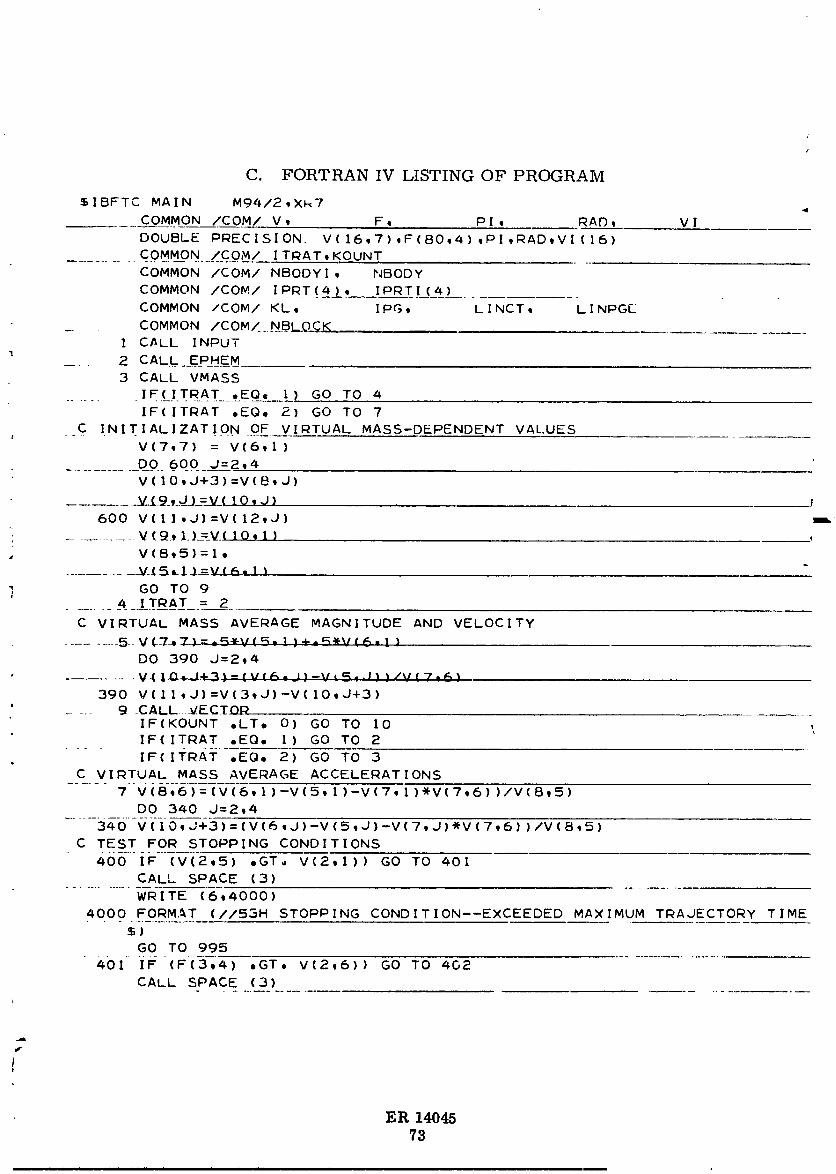
I

C. FORTRAN IV LISTING OF PROGRAM

$1BFTC MAIN M94/2,X_?

COMMON /COM/ V, F, PI, RAD, Vl

DOUBLE PRECISION. V(16,?),F(8Oi4),PI,RAD,VI (16)........ COMM_ON /COM/ iTRAT,KOUNT

COMMON /COM/ NBODYI _ NBODY

COMMON /COM/ IPR_T(4), IPRTI(4L_.COMMON /COM/ KL, IPG, LINCT, LINPG[

_ COMMON /COMZ_._BLO_E.I CALL INPUT

.... 2 CALL EPHEM

3 CALL VMASS

IF(ITRAT ,CO, I) GO TO 4

IF(ITRAT ,EQ, 2) GO TO 7

C INITIALIZATION OF VIRTUAL MASS-DEPENDENT VALUES

V(?,7) = V(6,1)

............ DO_ 600 J=2,4V(lO,J+3)=V(eiJ)

600 VIII,J}=V(12,J) _.--

. _..........V(gjI.}__V(IO,I )

V(8,5)=I,

............_-(5 LI_v c6 • I )

] GO TO 9.......__!IR_!_.: eC VIRTUAL MASS AVERAGE MAGNITUDE AND VELOCITY

DO 390 J=214

--V-(40_J eJ)-VtS_-I))/V(T,6)390 V(ll,J)=V(3_J)-V(IOqJ+3)

..... 9 _CALL__ECID-R

IF(KOUNT ,LT, O) GO TO I0 ,IF(ITRAT ,EQ, I) GO TO 2

• - " IF(ITRAT ,EOo 2) GO TO 3C VIRTUAL MASS AVERAGE ACCELERATIONS

? V(B,6)=(V(6,1)-V(5, I)-V(?,I)*V(7,6))/V(815)DO 340 J=214

340 V(IOqJ+3)=(V(6,J)-V(SIJ)-V(TIJ)*V(?,6))/V(BIS)C TEST FOR STOPPING CONDITIONS

400 IF (V(2t5) ,GT_ V(211)) GO TO 401CALL SPACE (3)

WRITE (614000)4000 FORMAT (//53H STOPPING CONDITION--EXCEEDED MAXIMUM TRAJECTORY TIME

$)GO TO 995

- 4bl" IF(F'(3,4) ,GT, V(2,6)) GO TO 402 ................CALL SPACE (3}

ER 1404573

ii i i ii i i i i

1966009743-082

W_ITE (614010)

4010 FOqMAT (//35H STOPPING CDhIDITION--IMpACTED EARTH)

GO TO 995

402 IF (F(7,4) ,GTI V(2,7)) GO TO 403 .. . ..........

CALL SPACE (3)

WRITE (5,4020)

4020 FORMAT (//35H STOPPING CONDITION--IMpACTED MOON )GO TO 995

403 CONTINUE

IF(KOUNT ,EQ, O) GO TO II

KOUNT = 0

I0 CALL PRINT

IF(KOUNT ,LT, O) GO TO I

11 CALL ESTMT

GO TO 5

995 KOUNT=-I

GO TO 10END

ER 1404574

i

1966009743-083

• IBFTCINP - -----:------:M94/2oXR-VSqBROUTINE INPUTCOMMON /COM/ V, F, PI, RAD, VI

__ DOUBLEI_PRECISiON V(16,7),FIBO,4),PI,RAD,VI (16)COMMON /COM/ ITRAT,KOUNT

COMMON /COM/ NBODYI, NBODY

COMMON /COM/ IPRT(4), IPRTI (4)

COMMON /COM/ KL, ........ IPG, LINCT, .....LINPGE ...........

COMMON /COM/ NBLOCK

.. COMMQN._/GCDIN/ ICARD(14)DIMENSION INCHK(6),FMT(2),CRDTYP(2,6),APRT(4),AAPRT(2,4),IX(3)

DIMENSION NBLK(4)

DOUBLE PRECISION WD(16)

EQUIVALENCE lWPD,WD(1)}

DATA INCHK /U,I_I, 1,0,! /

DATA NBLK /10,11,9,12 /

DATA FMT(1) /12H(A24,4D24,0)/

DATA CRDTYP (1,1) /12HPRINT /

DATA CRDTYP (1,2) /I2HPOSITION /

DATA CRDTYP (i,3} /12HVELOCITY /..... [

DATA CRDTYP (t,4) /I2HEFEMERIS /

DATA CRDTYP (i,5) /12HACCURACY /

DATA CRDTYP (I,6) /I2HSTOP /

DATA AAPRT /6H ,6H ,$ 6H ,6H I ,

$ 6H ,6H 3 /

DATA INER# /0/

DATA-P_INT / 6HPRINT /

DATA POSITI / 6HPOSITI /

DATA VELOCI- / 6HVELOCI /

DATA EFEMER / 6HEFEMER /

DATA ACCURA / 6HACCURA /

DATA STOP / 6HSTOP /DATA PROBLE / 6HPROBLE /DATA IENTRY /0/

IPG=O

KL=-77777

1 DO I0 I=I,{6

DO I0 J=l,7

I0 V(I,J)=O,

DO 20 I=I,80

DO 20 J=l,420 F( I,J)=O,

V( 3,5):VI(I)

V( 1,1)=VI(2)

V( 1,2)=VI(3)

V( 1,3)=VI(4)

V( 1,4)=VI(5)

V( 3,2)=VI(6}

#

ER 14045

75

!

1966009743-084

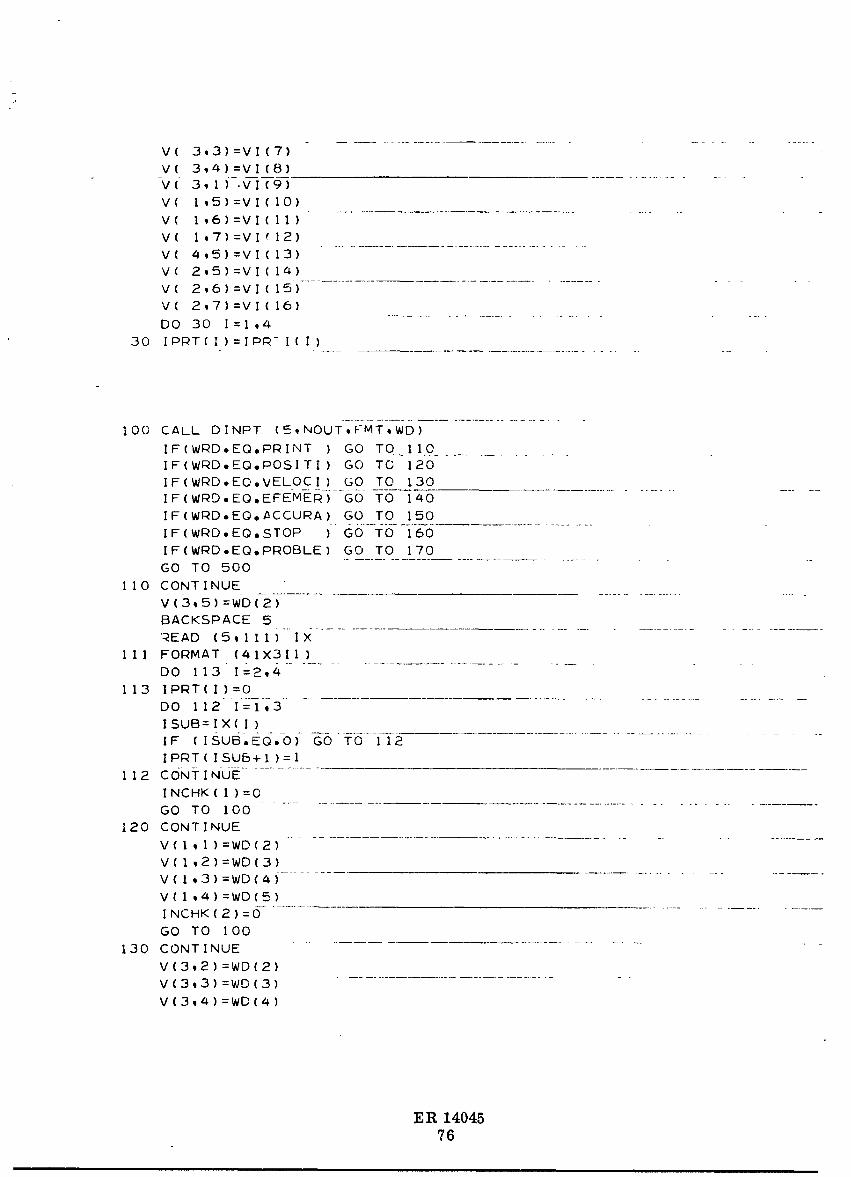
V( 3,3)=VI(7)

V( 3,4)=VI(8}

-V(" 3, l)--Vl(9) ..................

V( 1,5)=VI(IO)

V( 1,6)=VI(II)

V( 1,7)=Vl f12)

V( 4,5)=VI(13)

V( 2,5)=VI(14)

V( 2,6)=VI(15) ...........

V( 2,7)=VI(16)

DO 30 I=I,4

30 IPRT(1)=IPRTI(I)

100 CALL DINPT (5,NOUT-,FMT4WD)

IF(WRD,EQ,PRINT ) GO TQ,_IIIO___ ..................

IF(WRD,EQ,POSITI) GO TO 120

IF(WRD,EQ,VELOCI) GO TO 130

IF(WRD,EQ,EFE-MER) GO TO 140 ..............

IF(WRD,EQ,_CCURA) GO TO 150

IF(WRD,EQ.STOP )- GO--YO 160 .........

IF(WRD,EQ,PROBLE) GO TO I?0

GO TO 500

I10 CONTINUE

V(3,5)=WD(2)BACKSPACE 5'READ (5,111iIX ..........................................

Ill FORMAT (41X311)

DO I13 I=2,4I13 IP#T(1)=O

DO ! 12 "II_l;3 ...............................................

ISUB=IX(1)

IF (ISuB.EQ-,-b}-GO TO 112 .....................

IP_T(ISUB+I)=I

I 12 CoNTIN-UE ............INCHK( 1)=0GO TO 100

120 CONTINUEV(I,I)=WD(2)

V(I,2)=WD(3)

V(I,3)=WD(4)

V(I,4)=WO(5)

INCHK(2)=OGO TO lO0

130 CONTINUE

V(3,2)=WD(2)V(3,3)=WD(3)V(3,4)=WD(4)

ER 1404576

i

1966009743-085

m

............ /

INCHK(3)=OGO TO I00

140 CONTINUE

V(3,1 )=WD(2)

V(1,5)=WD(3)V(lo6)=WD(4)V(I_7)=WD(5)INCHK(4)=OGO TO 100

150 CONTINUE

V(4,5)=WD(2)INCHK(5)=CGO TO tO0

160 CONTINUEV(2,5)=WD(2)V(2,6)=WD(3)V(2,7)=WD(4)INCHK(6)=0GO TO |00

l?O CONTINUEKLT=WD(2) I

GO TO 600500 IF (INERR.NE,1) CALL NEWPGE

CALL SPACE (5)

WRITE (6,501)ICARD501 FORMAT (/56H AN ERROR HAS BEEN DETECTED READING THE FOLLOWING CARD

$--/10X,13A6_A2/18H EXECUTION DELETED/iH )INERR=I

GO TO 100

600 IF (IENTRY,NE,02 GO TO 650 ..................... ,,

DO 601 I=I,6

601 IF (INCH_IJLtNEtQ) GO TO 602 ...........

GO TO 649602 CALL NEWPGE ......

WRITE (6,604)

604 FORMAT (/91H THE FOLLOWING REQUIRED CARD TYPES WE__RRE NOT_ IN__PUT.QN..T

SHE FIFIST PROBLEM -- EXECUTION DELETED)

DO 605....[_lt6IF (INCHK(I),EQ,O) GO TO 605

WRITE .(.6t606) (CRDTYP(Jo_),J=I,2)606 FORMAT (lOX,2A6)605 CONTINUE .......................

INERR=I649 IENTRY=I

DO 610 I=1,4

610 IPRTI(1)=IPRT(1)

?,

ER 1404577

I

1966009743-086

I I

VI( I =V13,5)

VI ( 2 =V(I* I)

Vll 3 =V(I*2)

VI{ 4 =V(I13)

Vll 5 =V1144)

Vl( 6 =V(3,2)VI( 7 =V(3_3)

VI( 8 =V(_-_'_,_)VI( 9 =V(3,1)

VI( I0 =V(liB)vI(iI =v(i,6) .....VI( 12 =V(1,7)

VI(I3 =V(4,5)

VI(14)=V(2,5)VI(15)=V(2,6)

Vl(16)=V(2,7)650 IF (INERR.NE.O)- GO TO 100 ...........

NBODY=NBODYINBLOCK=O

DO 660 I=I,4

660 IF (IPRT(I).NEI-O)-_L LOCK=NBLOCK+NBLK(I) .................CALL NEWPGEKL=KLT

DO 651 i=I,4..........................................

J=IPRT( I )+1

651 APRT(1)=AAP_T(Jil)

WRITE (6,652) V(3,5),

$ APRTIV(1,1),(V(1,J),J=2,4) i(V(31J),J=21_)i

$ V(3, I),XV(1,J),J=5,7),V(4,5),(VI2,J),J=5*?)tKL652 FORMAT (12H PRINT 1PD20_I1_6X4A6/

$ 12H p6g-i-T ION 4D20. | I/ .........

$ 12H VELOCITY 3D20.11/_. +

$ 12H EFEMERIS 4D20.II/

$ 12H ACCURACY D20.11/

$ 12H STOP 3D20.II/

$ 12H PROBLEM 15)

CALL NEWPGE

C DIMENSIONAL CONVERSION FACTORS

V(IIS)=V(I,5)/RAD .....

V(4,7)=V(1,5)_V(li6)V(5,5)=V(4,7)_V(1,6}V(5,6)=V(5,B)_V(1,5)V(6,5)=V(5_6)*V(1,6)V(6,6)=V(615)_V(115)

ER 1404578

ii ii i i i

1966009743-087

,/

C EPHEMERIS DATA

V(1,7)=-V(1,7) ...........

V(5,?)=l,+V(1,7)

F(1_4)=V(5_7)

F(5_4)=-V(IQ?}

NBODY = 2

NBODY=4*NBODY L

C NONDIMENSIONALIZATION

DO 50 J=2t3

V(J_5)=V(Jo5)_V(I*5)

50 V(2tJ+4)=V(2_J+4)/V(I*6)

V(2,1)=V(I,I)*V(I_5)

V(4,1)=V(3_I)*V(Io5)

DO 51 J=2,4

V(2,J)=V(1,J)/V(1,6)

51 V(4,J)=V(3,J)/V(4,7)

C INITIALIZATION OF M-ISCELANEOUS VALUES

V(3,6)=DEXP(1,t3756474179255 + ,509713741462307*DLCG(V(4,5))

$ +,14560-181279278D-2 * DLOG(V(4,5))**2 )

ITRAT = 3 IKOUNT = i ..............

V(13,3)=V(2t 1)+V(3tS)

RETURN

END

il _p

ER 1404579

!

I

1966009743-088

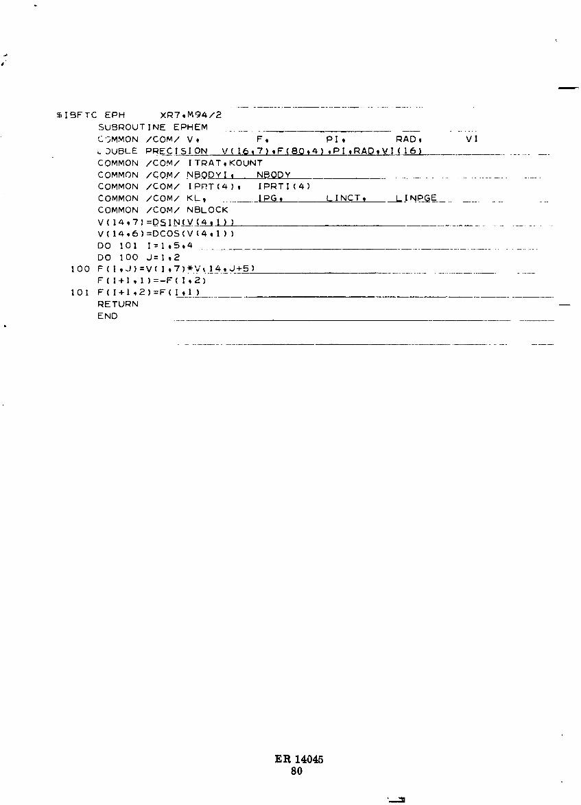
$1BFTC EPH XR?,M94/2SUBROUTINE EPHEM

C']MMON /COM/ V, F, Pl, RAD, Vl

_DUBLE PRECISION V(I6,?),F(80,4),PI,RADoVI,(16) .........

COMMON /COM/ ITPAT,KOUNT

COMMON /COM/ NBQ_I, NBODY ..................COMMON /COM/ IPRT(4), IPRTI(4)

COMMON /COM/ KL9 ..........IPG, LINCT_ __J.]NP_ ..............

COMMON /COM/ NBLOCK

V(14,?I=#SIN12_14,1) ) ..............V(14t6)=DCOS(V(4tl I )

O0 I0! I=1t514 ......................DO I00 J=l,2

100 F(I,J)=V(|,7)*.V__I_..tJ+5) .....F(I+I,I)=-F(I,2)

101 F(I+I,2)=F(I,I )

RETURN

END

ER 140458O

1966009743-089

/

$1BFTC VMS M94/2,X_7

SUBROUTINE VMASS .......

COMMON /COM/ V, F, Pl, RED, VI .-

DOUBLE PRECISION VI16,?I,FIB0_4) _PI_RAD,VI(16)COMMO_ /COM/-ITRA-oKOUNT

COMMOPI /COM/ NBODYI, NBODYCOMMON /COM/ IPRT(4) o IP_TI(4)COMMON /COM/ KL, IPG, LINCT, LINPGE

COMMON /COM/ NBLOCK

C VIRTUAL. MASS POSITION AND MAGNITUDE

V(12,5}=O,

DO 201 I=ItNBODYt4

DO 200 J=Io3

200 F(I+2,J)=V(2oJ+I)-F(IqJ)

F(I+2,4)=DsQRT(Fi-I+2,I)**2+F(I+2,2)**2+F(I+2,3}*'2)

F(I+3,4)=F(I,4)/F(I _2,4)*'3

201 v(I2,5)=v(12,B)-+F(I+3,4)

DO 203 J=1,3V(6,d+l)=O,

DO 202 I=I,NBODY,4202 V(6tJ+I)=V(6,J+I)+F(I+3_4)_F(I,J)

V(6,J+I)=V(6,J+I)/V(12_5)

203 V(IO,J+I)=V(2,J+-I)-V(6eJ+I)

V(IO,I)=DSQRT(V(IOo2}_*2+V(IO_3)w_2+V(IOq4)_2) "

V(6,1)=V(IO,1)_3_V(1205)

C VIRTUAL MASS VELOCATY AND MAGNITUDE RATE

V(12,6)=0,

DO 301 I=I,NBODY,4

DO 300 O&i,3 ........300 F(I+3,J)=V(4,J+I)_F(I+I4J)

F(I+I,4)=3,_(F(I+2_I)WF(I+3,1)+F(I+2,2)_F(I+3t2)+F(I+2,3)_F(I+3-3)

1)/F(I+2q4)*_2

301 V(12,6)=V(12,6)-F-(I+Io4)_F(I+3t4} \DO 303 J=I,3

V(8_J+I)=O,

DO 302 I=loNBODY_4

302 V(8,J+I)=v(SqJ+I)+F(I+3,4}_(F(I+IqJ)-F(ItJ)WF(I+I,_)}

V(8,J+I)=(V(8, J+I)-V(6,J+I)_V(12,6))/V(12oS)

303 V(12,J+I)=V(4tJ+I)'_V(SeJ+I)

I}/V(IO,I)_+V(I_,_)/V(I_,5))

RETURN

END

.........................

#,

ER 1404581

f

1966009743-090

• IBFTC VTR XR7,M94/2

SUBROUTINE VECTOR

COMMON /COM/ V, F, Pl, RAD, Vl

DOUBLE PRECISION V(16,7),FI80,4),P_,RAD,VIII61 .......................

COM_ION /COM/ ITRAT,KOUNT

COMMON /COM/ NBODY[_ .... NBODY ...................

COMMON /COM/ IPRT(4), IPRTI (4)

COMMON /COM/ KL, II IPG, LINCTt LINPG_E .......

COMMON /COM/ NBLOCK

C VECTOR ORBITAL ELEMENTS ............... ............

DO 401 J=2,4

DO 400 I=9,11,2 .........................

400 V(l,J+3)=V(I,J)

401 V(16,J)=V(9,J+l}*V(ll_J+2)-V(g,J+2)*V(lloJ+l__)

DO 403 J=2,4

DO 402 I=11,16,5..............................

402 VII,J+3)=V(I,J)

403 V(14,J)=-V(9,J)/V(9_t}-(V(16,J+l)*V(lI,J+2)-VI16,J+2)*V( lloJ+l))/V

I(7,7)

DO 404 I=14,16,2

V(l,5):V(l,a)*_a+V(I,3)_a+V(I,4)**2

404 V( I, I )=DSQgT(V(I,5) ) ......

V(13,5)=I,-V(14,5)

V(13,6)=DSQRT(DABS(V(13,5)))

V( 13,7)=V( 16,5)/V(7,7}

IF (ITRAT,EO,3) RETURN

C SPACECRAFT FINAL POS-iTION AND VELOCITY

V(6,7)=V(7,6)+V(7,6)*V(7,6)*V(6,7)

DO 410 J=2,4

410 V(9,J+3)=V(9,J)+V(6,7)*V(l 1,J)

V(8,7)=V(13,7)/(V(14,2)wV(9,5)+V( 14,3)wV(gQ6)+V(14,4)wV(9,7)+DSQRT

DO 411 J=_,4

411 V(IO,J)=V(B,7)*V(9,J+3)

V(lO,1)=DSQRT(V(IO,2)**2+V(lO,3)**2+V(lO,4)**2)

DO 414 J=2,4

414 V(Ia,J)=V(14,J)+V(IO,J)/V(IO,I)

DO 413 J=2,4

DO 41a ........................412 V(I,J+3)=V(I,J)

V(Ia,J)=(V(16,J+I)*V(12,J+2)-V(16,J+a)*V(Ia,J+I))/V(13,----#) ..............

V(2,J}=V(tO,J)+V(6,_J)

413 V(4,J)=V(12,J)+V(lO,J+3)

C KEPLERIAI4 TIME OF FLIGHT

IF(VII4,1) ,NE, 0,) GO TO 501

500 M=9

GO TO 502

501 M:I4

502 NN:I6-M

D0 504 J:2,4O0 503 I=M,16,NN .....................

ER 1404582

1966009743-091

l

"--"

503 V(I.J+3)=V(I,J)

504 V¢II.J+3)=(V(16.J+I)*V(M,J+2)-V(M,J+I)*V(16,J+2i)/(VIIS, I)*V(M.i)) /

DO 517 I=9,10

............................

IFlV(13,51 oEQ, C-) GO TO 506505 VII+CQ5)=V( 13,7)/V(13.6)

GO ,0 507

506 V( I+6,5)=2./(V(I,!_-V( 13,71 )507 V(l+6,5):(V(ll,5)*Vll,2)+V(ll,6)*Vll,3)+V(ll,?)*V(i,4)-)/V(_+6,5)

IF(VII3,5)) 508,509_510508 VII+6,6)=DLOG(V(I+6,5)+DSQRTIV(I+6,5)**2+I.))

GO TO 517

509 V(l+6,6)=V(14,1)**2*lV( 13,?)*VI I+6,5))*'3/3,

GO TO 517 ..........510 IFIDABS(V(I+6,5)) .LT. 1.) GO TO 524

IF (DA_SIV(I+6,5)) ,LE, 1,0001) GO TO 597

KOUNT:-I

CALL SPACE (2)

WRITE (6,596)596 FORMAT (/27H UNACCEPTABLE ERROR IN ATAN)

RETURN

597 CALL SPACE (2)

WRITE (6,598) ..... I598 FORMAT (/27H ACCEPTABLE ERROR IN ATAN)

V(I+6,6)=DSIGNIPI/2.,V(I+6.5)) ............. 'GO TO 523

524 VII+6,6)=DAT#N(V-(-I+6,B)/DSQRTII.-V(I+6.5)**2)) ........ "

523 IF(V(I_,I) .. [. 0.) GO TO 512

511 V(l+6,7)=V(,,2)*V(9,2)+V(l,3)*V(9,3)+V(l,_)*V(9,_)

GO TO 513512 V( I+6,7)=V( 13,?-)/V(13,5)-V(1,1) .......513 IF(V(I+6,7) ,GE, 0,) GO TO 517

IF(VfI+6,Si--.G-E, 0.) "0 TO 516V(I+6,6)=-P-I-V(I+6,6) _'

GO TO 517516 V(I+6,6)=PI-V(I+6,6)

_L

517 CONTINUE .............IF(V(13,5) ,EQ, 0,) GO TO 519

VlS,Tl=VlT,7)@*2/V(16,1)**3*V(13,5)*V(13o6) ........... --GO TO 520

519 V(8,7)=V(16,l)*V(14,1)**2/2_ ......

520 Vl?,5)=V( 16,6)-V(15,6)+V(14,1)*lV(15q5)-V(16,5)}

IF(V(?,5) ,GE, 0o) GO TO 522

IF (v(e,?),LT,0,) GO T0 522

V(?,5):V(TCS-}#2.*Pl ...........

522 V(?,5)=V(7,B)/V(8,?}UPDATE ESTIMATEOF_CURVE

IF (V(T,5),EQ,O,) GO TO 525

V{6,7)=(V(6,T)_V(7,5) )/V(?,5)** 2 - ,525 RETURN

END .........

o ER 140 ,83

1966009743-092

_IBFTC P_T X:7,M94/2

SUB_OUT I NE P#INTCO_MOlg /CO_/ V, .... F, Pl . RAD, Vl

DOUBLE PRECISION V( 16,7),F(80,41 ,PI_RAD,VI(16)

COMMON /COM/ IT#AToKOUNT

COMMON /COM/ NBODYI, NBODY

• COMMON /COM/ IP#T(4}, IPRTI(4)

COMMON /COM/ KL, [PGt .... L I._C_3___ LINPG_E ....COMMON /CO_/ NBLOCK

DOUBLE PRECIS!ON TEMP(16),RV,VV,RS.VS......................

DO 351 J=2,4

DO 350 I=1,5,4VII,J)=V( 1,6)*V( l+l,J}

V(I+2,J}=V(4,7)_V(I+3,J)

F(I,J-I I=V(I,6}*F(IiJ-I}

350 F(I+],J-I)=V(4,?)*F(I+I,J-I)

35I CONTINUE

DO 352 J:],4352 V(|5,J)=V(SiS)_V(-16tJ)

V(I,l ):V(2, I)/V(I,5)

V(3,I )=VI4,1)/V(I,5)

V(5,l}:V(6,1)*V{6,5}

Vl?,l):V(B,l)*V(6,6)

RV:DSQ#T(V(5,2}**2+V(5,3)**2+V(5=4}**2)

VV:DSORT(V(?,2)**2+V(?,3)**2+V(?,4)_2}

RS:DSQRT(V(I,2)**2+V(],3)*_2+V(I,4}**2}

VS=DSQRT(V(3,2}**2+V(3,3}*w2+V(3,4)*_2) "410 CALL SPACE (NBLOCK)

WRITE (6,411-) (V(I,II,I=I,4},RS,(V(3,1I,I=2,4),VS .....

411 FORMAT (I/III20H TRAJECTORY TIME = IPD20-|I//$ 4 OH SPACECRAFT INERT IAL TRAJECTORY /

$ 40H POSITION . . • . . . . . . . . . . 4D20. I I/$ 40H VELOCITY • , • o • • • • • • • • . 4D20.II)

420 IF (IPRT(2),EG_O} GO TO 430. _._.

TEMP( I) = F(I,I)

TEMP( 2} = F(I ,2)

TEMP(3 ) = F(I,3) ..............

TEMP(4) =DSQRT(TEMP(I}**2+TEMP(2)_*2+TEMP{3}**2}

TEMP( 5} = F(2-,-I) .....

TEMP{6 ) = F(2,2)

TEMP( 7} = F(2,3} ..........

TERP(8) =DSQRT(TEMP(5}**2+TEMP(6)**2+TEMPI?)**2)

TEMP( 9) : F(5,I) .........

TEMP(IO) = F(5,2)

TEMP(11} = F(5,3}

TEMP(12)=DSQRT(TEMP(g}**2+TEMP(IO}**2+TEMP(II)**2}

TEMP(13) = Fi6,i-i ...........

TEMP(Ia} = F(6,2}

TEMP{15) = F(6,3)

TEMP(16}=DSQRT(TEMP(13}**2+TEMP(14)*_2+TEMP(15}_*2)

WRITE C6,42I} V(3_-_,(TEMP(1),I=I,]6} ........

421 FORMAT (/// 20H EPHEMERIS TIME = IPD20,II//

$ 40H EPHEMERIS DATA /

$ 40H POSITION OF EARTH , , , , • • , , 4D20,11/

ER 1404584

1966009743-093

$ 40H VELOCITY OF EARTH- . . • . • , . . 4DZC. I 1//$ 40H POSITION OF MOON • • • • • t • . 4D2011 I/

$ 40H VELOCITY OF MOON , , , , , , , , 4D2C,II) '

430 IF (IPRT(3),EO,O) GO TO 440TEMP ( I ) = V(I,_}-F(I,I)

TEMP ( 2) = V( 1.3)-F(1,2)TEMP (3) = V-iI-,4)-F(I13)

TEMP( 4)=DSQRT(TEMP(I )*_2+TEMP(2}**2+TEMP(3)**2)

TEMP ( 5) = V(3,2)-F(2,1)TEMP ( 6) = V(3,3)-F(2,2)TEMP ( 7) = V(3•4)-F(2,3)TEMP( e)=DSQRT(TEMP(5)**2+TEMP(6)**2+TEMP(7)*_2)TEMP (9 ) = V(1.2)-F(5,1) ....TEMP (}0) = V(|43)-F(5,_)TE_P (11) = V(1_4)-F(513) -rEMP(12)=DSQRT(TEMP(9)_*2+TEMP(IO)**2+TEMP(ll)**2)

TEMP (13) = V(3,2)-F(6tl)TEMP (14) = V(313)-F(612)

TEMP (15) _- V(394)-F(6_3) i

TEMP(I6)=DSQRT(TEMP(13)*_2+TEMP(14)*_2+TEMP(15)_*2)WRITE (6,431) (TEMP(I)tI=lI16)

431 FORMAT(/// 40H SPACECRAFT RELATIVE TRAJECTORIES /$ 40H POSITION REL, TO EARTH • , , i , • 4620,11/ --$ 40H VELOCITY REL, TO EARTH , , , , , , 4D20,II/I

$ 4OH POSITION REL, TO MOON • . • • . •-#D26,11/

$ 40H VELOCITY REL, TO MOON • , , , , , 4D20,II )

440 IF (IPRT(4),EQ.o) RETURN ..........

TEMP(1)=V( 9,2)*V(I,6)

TEMP(2)=V(-gI3)*V(I,6) .....TEMP(3)=V( 914)*V(1,6)TEMP(4)=V( 9.1)_V(1,6)TEMP(5)=V(Ili2)_V(4qT)TEMP(6)=V(li.3)_V(-_7) .......TEMP(7)=V(llI4)_V(4,7)TEMP(8)=DSQRT(TEMP(5)_2+TEMP(6)_2+TEMP(?)wW2) .........WRITE (6,441) (V(5, I},I=2,_),RV,(V(7, I),I=2,4),VV,

$ (TEMP(1),I=I,8),

$ (V(15,1),l=2,4),V(15,1)i(V(14,1),l=2,4)•V(14,1),

$ VlSll)iV(7,1)441 FORMAT(/// 20H VIRTUAL MASS DATA /

$ ........--4EH" VIRTUAL MASS POSITION , , , , , , 4{-I-l_D_O,i-I

$)/ 40H VIRTUAL MASS VELOCITY • , • , , , 4D20,II/

$ - 4OH SPACECRAFT POS. REL'. TO V.M. • . . _D20.IlI/--

$ 40H SPACECRAFT VEL. REL. TO V.M. • . . 4D20,11/$ - _OH KEPLER (ANG. NON.) VECTOR. • . . . 4_0.1I-7 -

$ 40H ECCENTRICITY VECTOR • • , • , , , 4D20,111

$ "-2-4H V,M, MAGN, = D20,11/ .........

$ 24H V,M, MAGN, RATE = D20,11)RETURN

- END

._ ER 14045<'. 85t;

] 966009743-094

$1BFTC EST XR?,M94/2

SUBROUTINE ESTMT ..........................

COMMON /COM/ V, F, Pl, RAD, Vl

DOUBLE PRECISION V(li6tT)itF(B0t4ii}iPltRADIV.I(16 ] ............

COMMON /COM/ ITRAT,KOUNT

COMMON /COM/ NBODYI t NBODY___ ..............COMMON /COM/ IPRT(4), IPRTI(4)

COMMON /COM/ KL, IPG., LINCT, ...._INPGE_

COMMON /COM/ NBLOCK

C INDEX VALUES IN V ARRAY...........................

DO 361 I=I,912

DO 360 J=l,4 .....................

360 V(I,J)=V(I+I,J)

361 CONTINUE

ITRAT=I

C ESTABLISH COMPUTING TIME INCREMENT

395 V(13,4)=V(TiS)*V(1615)/(V(1515)-V(16,5))IF (V(7,6).EQ, O,) V(13+4)=-I,

V(II,I)=DSQRT(V(II,2)**2+V(II,3)**2+V(III4)**2)

V(?_6)=V(3,6)*V(9,1)/V(IIII)

IF{V(1314) ,LT, 0,) GO TO 394

IF(V(1314) _GT, 1,1"V(7+6)) GO TO 394

V(Ti6)=V(13,4)

CALL SPACE (5)

WRITE (6,6000)

6000 FORMAT (//2X,19HMAJOR AXIS CROSSING//IH )

GO TO _O03g4 IF(Vil.l)+l.l*V(716) .LT. V(i313)) GO TO 378

390 V(746)=V(13,3)-V(l, 1)V(13,3)=V(1313)+V(3,5)

400 KOUNT = I

C INCREMENT TIMES

3?8 DO 379 I:I1312

_79 V(I+I_I)=V( l_i )+V(7,6)

V(8,5)=V(7,-6)**2 ...............

IF (V(2,1),GE,V(!3,3)) V(13,3)=V(13.3)+V(315)

C ESTIMATE VIRTUAL MASS FINAL POSITION AND MAGNITUDE

V(6,1)=V(5,1)+V(?,I}*V(?.6)+V(B,6)*V(815)

DO 380 J=2,4380 V(6_J)=V(5,J)+V(?qJ)*V(?,6)+V(10_J+3)_V(StS)

RETURNEND

ER :1.404586

I

1966009743-095

/

$1BFTC BLKDAT XR7 oM94/2

BLOCK DATA

COMMON /COM/ V, F, Pl, ---gAD, Vl .

DOUBLE PRECISION V(16,'7}QF(80,4),PI,RAD,VI(16)

COMMON /COM/ ITRAT,KOUNT

COMMON /COM/ NBODYI, NBODY

COMMON /CON/ IPRT(4), IPRTI(4) '-

COMMON /CO_/ KL, IPG, LINCT, LINPGE

COMMON /COM/ NBLOCK

DATA Pl /3,141592653589793 /

DATA RAD /57,29577951308232 /

DATA NBODYI / 2 /

DATA IPRTI / I,O-,oQo /

DATA L INPGE/60/

DATA Vl / 5,DO, IIWO,DO, I,D-?, 3_O,DO /

END

..

I

ER 1404587

!

1966009743-096

P

$1BFTC DIN XR?,M94/2

SUBROUTINE DINPT (X_XX, XXX,WD)DOUBLE PRECISION WD(5)

COMMON/GCDIN/ !CARD(14) .............

READ (5_1) ICARDI FORMAT (13A6,A2)

BACKSPACE 5

_EAD (5,2) WD2 FORMAT (A6,2X.4DIB,O)

RETURNEND

ER 14O4588

1966009743-097

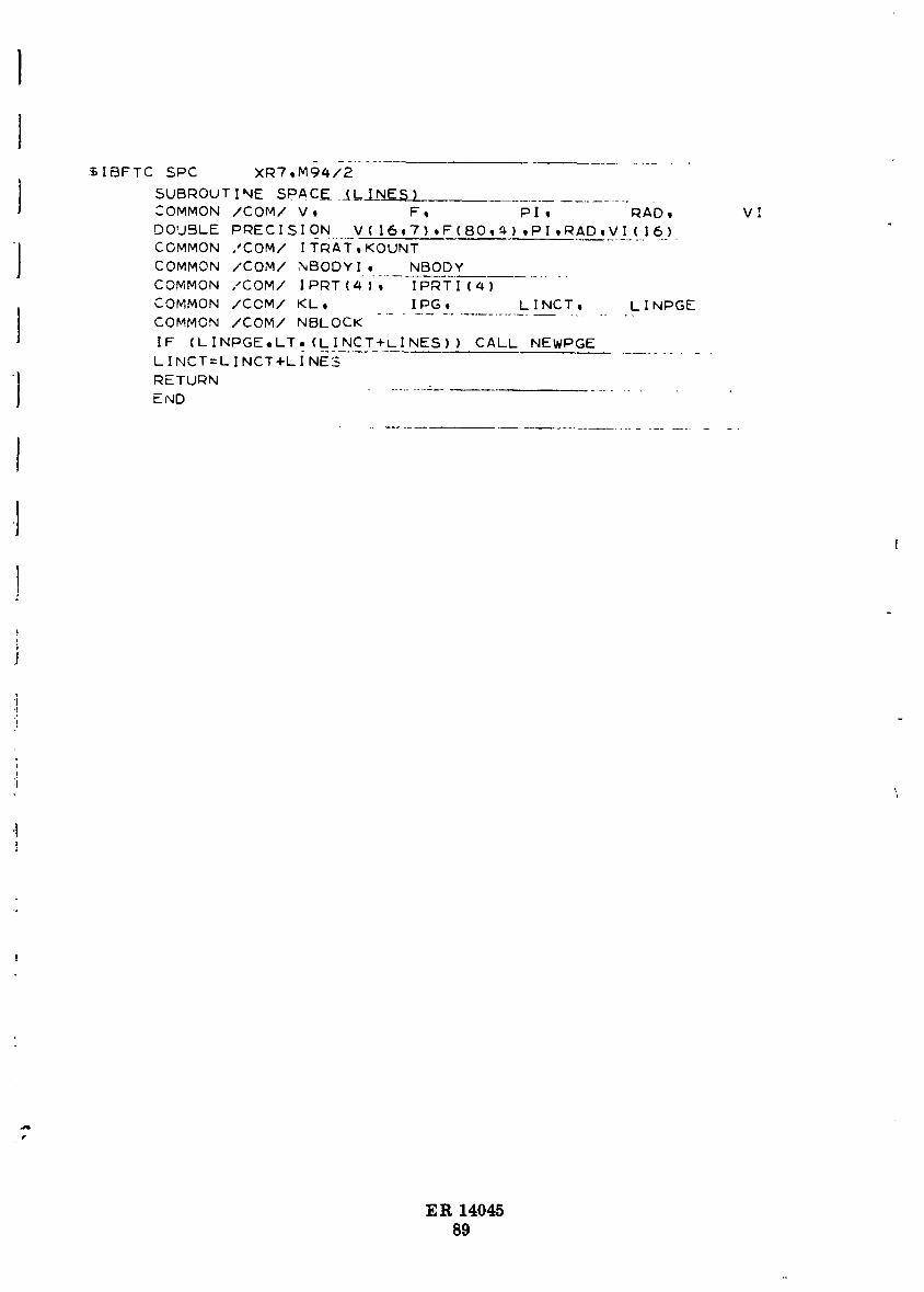
I• XBFTCSPC XR_,Mg_22.........

SUBROUTINE SPACE_Sb]_._E_,.S_}COMMON /COM/ V, F, Pl, RAD, Vl

DOUBLE PRECISION V(16,7),F(80,_},PI,RAD,VI (16)

-J COMMON ,'CON/ ITRAT,KOUNT

1 COMMON /COM/ NBODYI., ...... NBODY ......COMMON /COM/ IPRT(4), IPRTI(4)

COMMON /COM/ KL, IPG, LINCT, LINPGE

I ...........................

COMMON /COM/ NBLOCK

IF (LINPGE,LT, (LINCT+LINES) } CALL NEWPGE

LINCT=LINCT+LINES ..........

"Ii RETURN .......... =........i END

1I

]

A

ER 1404589

1966009743-098

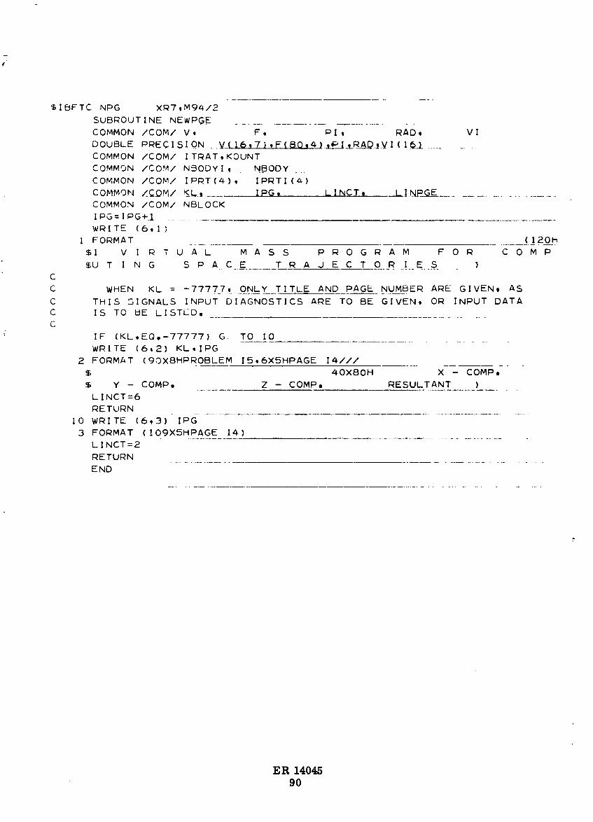
$1BFTC NPG XR7,M9412

SUBROUTINE NEWPGE ..............................

COMMON /COM/ V, F, Pl, RAD, Vl

DOUBLE PRECISION .._(16,7},F(BO,4J.L__tR_.lYI(I_ ........

COMMON /COM/ ITRAT,KOUNT

COMMON /COM/ NBODYI _ NBOOY _._COMMON /COM/ IPRT(4), IPRTI (a)

COMMON ZC.OM/ _I I IPG, .. LINCT, L!.NRGE ..........................COMMON /COM/ NBLOCK

IPG=IPG+I ......WRITE (6,1)

I FORMAT (120_

$I V I R T U A L M A S S P R 0 G R A M F 0 R C 0 M P

SU T I N G S P A C E T R A J E C T 0 R I E S )

C

C WHEN KL = -7777]_._ON_Y TITLE AND PAGE NUMBER ARE GIVEN, AS

C THIS SIGNALS INPUT DIAGNOSTICS ARE TO BE GIVEN, OR INPUT DATAC IS TO UE LISTED,

C

IF (KL,EQ,-77777) G- TO I0

WRITE (6,2) KL,IPG

2 FORMAT (90X8HPROBLEM 15,6XSHPAGE 14///

$ 40X80H X-_ COMPo -

$ Y - COMP, Z - COMP, RESULTANT )

LINCT=6

RETURN

I0 WRITE (6,3) IPG

3 FORMAT (I09XSHPAGE 14)

LINCT=2

RETURN.............................

END

ER 140459O

1966009743-099

/

VII. CONCLUSIONS AND RECOMMENDATIONS

A. CONCLUSIONS

The results of this study have shown that the virtual mass techniqueprovides a practicable and very flexible method for solving the n-bodyproblem. Identically.the same computer program can be controlled bya single input tO obtain approximate solutions very quickly, or highlyaccurate trajectories in a proportionately longer time. The sample cir-cumlunar trajectory included in thi_ report gives the spacecraft positionaccurate to within 0.02 naut mi at t = 70 hr (approximately 0.33 h_ be-fore pericynthion) in 160 sec on an IBM 7094 digit:_l co_,puter.

The use of rectangular coordinates and the formulation of the conic

section relationships in terms of the vector orbit:d elements k, e haveresulted in a computationally con_pact program. Without the elaborateinput-output provisions which haw, been incorporated to provide oper-ational flexibility, the basic computational program easily fits in anIBM 1620 computer.

I

B. RECOMMENDED FUR_[HER STUDIES

A number of further studies are suggested and will be listed herewithout elaboration.

(1) Derive analytical expressions for trajectory sensitivitiesfrom the simple conic section forms relative to the virtualmass. Use these to propagate the state transition matrixanalytically.

(2) Study techniques for representing aspherical gravitational po-tentials by appropriate planet-fixed distributic',ns of discrete ,point masses similar to the method of Ref. 4. Investigatethe integration of such trajectories by _he virtual mass tech-nique.

(3) Study the problem of computing dynamically consistent tra-jectories (see Refs. 2 and 5) by investigating an extension ofthe virtual mass technique to compute the simultaneous tra-jectories followed by n gravitating bodies. The procedurewould be to reduce the problem to a series of n two-body sys-tems at every instant. Each two-body system would consistof a different one of the n real bodies and a correspondingfictitious body lumping the effects of all others on the one ofimmediate interest. The numerical computation accuracywould be controlled so as to conserve known integrals: energy,momentum and uniformity of motion of the center of mass.

ER 1404591

1966009743-100

(4) Develop an Encke-like procedure for computing low thrusttrajectories. Here the thrust perturbation would be inte- ,grated separately and added as a correction to the referencegravitational trajectory relative to the virtual mass.

(5) Perform a general study of trajectories of the virtual massto ascertain, if possible, the fundamental characteristics ofits motion. Also try to find an analytical solution to the vari-able mass two-body problem.

ER 1404592

1966009743-101

/

VIII. REFERENCES

1. Gartmann, H. "Raumfahrtforschung." R. Oldenbourg, Munchen,1952.

2. Novak, D. "Two-Body Midcourse Navigation and Guidance forLunar Missions." AIAA Preprint No. 64-649, AstrodynamicsGuidance and Control Conference, Los Angeles, August 1964.

3. Miner, W. and Sperling, H. "The Varicentric Method of SpaceFlight Calculations with Introduction of the Ephemerides." MSFCReport No. DA-TM-93-59, December 1959.

4. Vinti, John P. "Theory of an Accurate Intermediary Orbit forSatellite Astronomy." Journal of Research of the National Bureauof Standards, B. Mathematics and Mathematica.t Physics, Vol.65B, No. 3, July-September, 1961.

5. "Explanatory S.lpplement to the Ephemeris." Her Majesty' sStationery Office, London, 1961.

ER 1404593

|

1966009743-102