shoni2.princeton.edushoni2.princeton.edu/ftp/lyo/dpw/pom_v06.docx · web viewthis book is about...

Geophysical Fluid Experiments with the Princeton Ocean Model

Lie-Yauw OeyPrinceton University

Dong-Ping WangStony Brook University

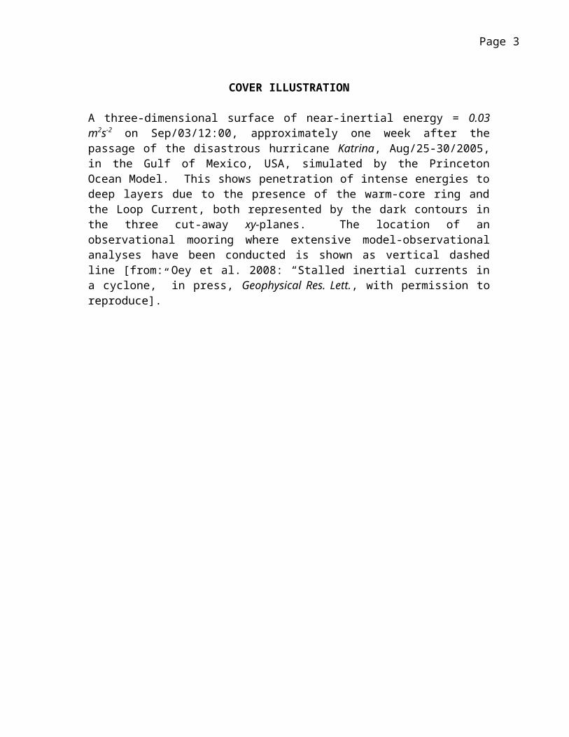
COVER ILLUSTRATION

A three-dimensional surface of near-inertial energy = 0.03 m2s-2 on Sep/03/12:00, approximately one week after the passage of the disastrous hurricane Katrina, Aug/25-30/2005, in the Gulf of Mexico, USA, simulated by the Princeton Ocean Model. This shows penetration of intense energies to deep layers due to the presence of the warm-core ring and the Loop Current, both represented by the dark contours in the three cut-away xy-planes. The location of an observational mooring where extensive model-observational analyses have been conducted is shown as vertical dashed line [from: Oey et al. 2008: “Stalled inertial currents in a cyclone,” in press, Geophysical Res. Lett., with permission to reproduce].

PROLOGUE: About This Book

“.. I have no special talents. I am only passionately curious..” (Albert

Einstein)

This book is about exploring various aspects of fluid motions on a

rotating earth using a popular, relatively simple yet powerful numerical

model - the Princeton Ocean Model (POM). It is a book aimed primarily for

advanced undergraduates and graduates in physical oceanography; but the

book should also be useful for researchers or anyone fascinated by and

intensely curious about oceanic fluid motions. Some knowledge of fluid

mechanics is assumed, equivalent to a two-semester course which usually

covers up to the derivations of conservation laws of viscous fluid motions,

including the boundary layer theory; these prerequisites should not be an

impediment to those interested enough to want to open this book. On the

other hand, we have strived to make the book more or less self-contained by

building each chapter from simple to more advanced concepts. By

conducting geophysical fluid experiments on a computer and analyzing the

results, we hope that the student will gain a solid understanding of

geophysical fluid dynamics (GFD) and physical oceanography; the student

will also learn to critically examine the results (be a skeptic) and to attempt

connecting them to the real-world phenomena. And of course, the student

will learn to use POM, numerical methods and, we hope, to keep exploring

long after he or she surpasses this book.

Why POM? One reason is our familiarity with the model. More

importantly, however, it is because the model is relatively easy to tweak, say

to suit a different flow problem, or to change the model physics. This makes

it an excellent educational tool because it gives the student a hands-on

experience. It is much like the difference between being a driver and being

a driver as well as a mechanics. Most of us are the former, but only the

privileged few belong to the latter. POM shares many of the same features

of other popular ocean models now available in the scientific community,

and it uses basically the same equations of motions and conservation of mass

etc. Therefore, an accomplished student of this book should find it easy to

transit to other models should he or she so desire.

The book begins in chapter 1 with the near-surface ocean response to

wind built upon Ekman’s fundamental work. This is not the common

approach of a book in physical oceanography. On the other hand, most of us

experience the ocean perhaps through a summer swim in a coastal sea or in a

lake, and wind-driven surface motions are the most apparent. For a majority

of flows on the rotating earth, we find that by directly dealing with viscous

boundary-layer (i.e. Ekman’s) flows, one can quickly grasp why most of the

ocean’s interior is nearly inviscid yet why the boundary layers are so

important for the interior flows.

POM and related files for exercises outlined in this book can be downloaded

from:

ftp://aden.princeton.edu/pub/lyo/pom_gfdex/

Download latest public-released POM from:

http://www.aos.princeton.edu/WWWPUBLIC/PROFS/waddownload.html

Download POM User Guide other releases from:

http://www.aos.princeton.edu/WWWPUBLIC/htdocs.pom/

http://www.aos.princeton.edu/WWWPUBLIC/htdocs.pom/

http://www.aos.princeton.edu/WWWPUBLIC/PROFS/waddownload.html

ftp://aden.princeton.edu/pub/lyo/pom_gfdex/

CHAPTER 1: Wind-Driven Ocean Currents

The book begins with the near-surface ocean response to wind. We

will for the moment assume that the ocean density ( 1035 kg m-3) is

constant. Throughout this book, unless explicitly stated, we will use the SI

units. Most of us experience the ocean perhaps through a summer swim in a

coastal sea or in a lake. Wind-driven surface motions in the form of waves

and surfs are familiar. However, these motions can involve large vertical

accelerations and are of very small scales (order of centimeters to meters,

O(cm-m)) which we will not model for now, at least not directly. Instead,

we focus on motions which are of sufficiently large scales in the horizontal

(scale L ~ O(1-1000 km)) compared to vertical (scale D ~ O(10-1000 m)),

D/L << 1, that the pressure field satisfies the hydrostatic equation:

∂ p∂ z

=−ρg, (1-1)

where a Cartesian coordinate system xyz is used such that, conventionally, x

and y are the west-east and south-north axes respectively, and z is the

vertical axis with z = 0 placed at the mean sea level (MSL; Figure 1-1); x, y

and z are measured in m. The pressure p is in N m-2 (also called Pascal, Pa),

and g ( 9.806 m s-2) is the acceleration due to gravity. In other words, the

motions of interest occur in such thin fluid layers (with D/L << 1) that as far

as the vertical force balance is concerned the fluid may be treated as being

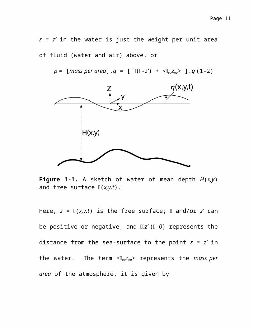
static.1 For such an atmosphere-ocean system, the pressure at some depth z =

z’ in the water is just the weight per unit area of fluid (water and air) above,

or

p = [mass per area].g = [ (-z’) + <eazea> ].g (1-2)

Figure 1-1. A sketch of water of mean depth H(x,y) and free surface (x,y,t).

Here, z = (x,y,t) is the free surface; and/or z’ can be positive or negative,

and z’ ( 0) represents the distance from the sea-surface to the point z = z’

in the water. The term <eazea> represents the mass per area of the

atmosphere, it is given by

<eazea> = ∫❑

∞

❑adz ∫0

∞

❑adz (1-3)

1 The thinness of the oceanic (or atmospheric) layer is comparable to that of the sheet of paper of this book.

where a is the air density. Thus ea and zea may be thought of as the effective

density and height of the “air-containing” atmosphere. The main bulk

(about 80%) of the atmosphere’s mass is within the lowest layer (the

troposphere) of about 10 km thick such that the atmospheric pressure at the

sea surface, pa = <eazea>.g 105 N m-2 = 1 bar.2 Equation (1-2) can be

written as

p = g(-z’) + pa(x,y,t) (1-4)

which is also obtained by integrating (1-1) from z = z’ to z = ; in general,

the pa is a function of the horizontal position and time.

If both a and pa do not vary with (x, y) and either are steady or at most

only vary so slowly with time that the fluid remains in hydrostatic

equilibrium, i.e. (1-1) is satisfied, then the fluid remains motionless provided

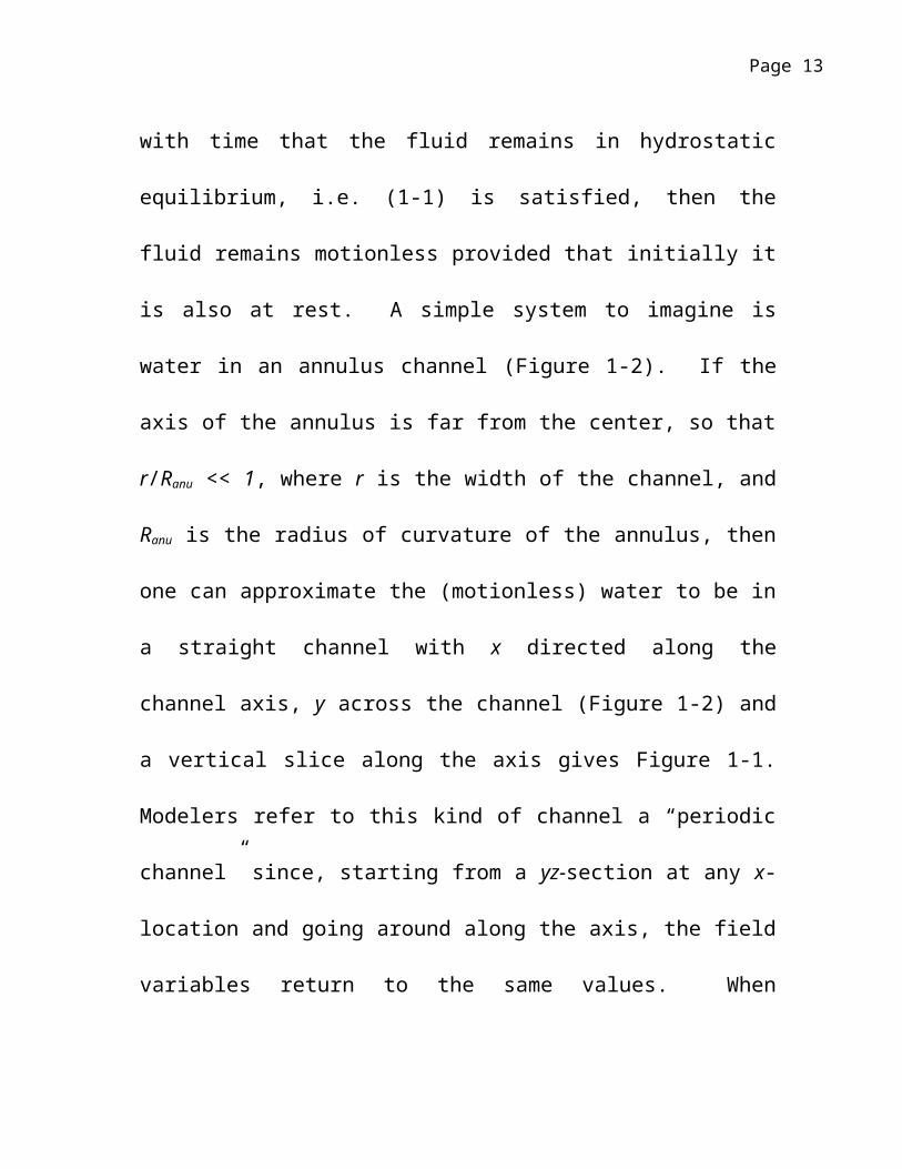
that initially it is also at rest. A simple system to imagine is water in an

annulus channel (Figure 1-2). If the axis of the annulus is far from the

center, so that r/Ranu << 1, where r is the width of the channel, and Ranu is the

radius of curvature of the annulus, then one can approximate the

(motionless) water to be in a straight channel with x directed along the

channel axis, y across the channel (Figure 1-2) and a vertical slice along the

2 An easy way to remember this is to use ea 1 kg m-3, zea 10 km and g 10 m s-2. Note also the familiar weather reporting of “1000 millibar” etc, which is 1 bar, the approximate sea-level pressure.

axis gives Figure 1-1. Modelers refer to this kind of channel a “periodic

channel” since, starting from a yz-section at any x-location and going around

along the axis, the field variables return to the same values. When

conducting geophysical fluid experiments, a periodic channel is a convenient

configuration to use because it often allows the extraction of essential flow

physics while at the same time alleviates the modeler from having to

formulate more complicated boundary conditions.

Figure 1-2. A circular annulus channel of radius Ranu much larger than the width of the annulus r. This is used to illustrate along-channel periodic fluid motion within the annulus.

1-1: A Simple Shearing Flow by the Wind

Consider therefore the straight channel (Figure 1-1) in which we will

further assume that all variables are independent of the cross-channel axis

“y,” and that the earth’s rotation is nil. The flow is described by the three

components of velocity (u, v, w) and the pressure p. Since there can be no

flow across the channel wall, i.e.

v = 0, at y = 0 and y = r, t. (1-5)

the cross-channel velocity v must be zero everywhere; the symbol t means

“at all time.” The channel is further idealized by letting its depth H =

constant. Initially, at t = 0, the water is at rest. A wind stress (N m-2) is

then applied uniformly at the surface, so that is a function of time only:

= (t) (1-6)

Similarly, we could stipulate that pa is also a function of time only; but for

simplicity we will set

pa = 0. (1-7)

It follows that, the along-channel velocity u cannot vary with x. Therefore,

at any point, there can be no accumulation (convergence or divergence) of

mass, and since w = 0 at z = H, the vertical velocity is nil everywhere, and

the sea-surface remains flat. Thus,

u = u(z, t), w = 0 = /x = p/x. (1-8)

Under these very specialized conditions, a parcel of fluid experiences

acceleration only due to the vertical shear stress. The momentum balance is

then:

DuDt

=∂❑zx

∂ z (1-9)

where zx denotes shear stress (force per unit area) in the x-direction acting

on the fluid elemental face that is perpendicular to the z-axis, and D(.)/Dt is

the material derivative which for a fluid property S is given by

DSDt

=∂ S∂ t

+u ∂ S∂ x

+v ∂ S∂ y

+w ∂ S∂ z . (1-10)

For the present specialized case, the last three terms are nil, and with S = u,

we have DuDt = ∂u

∂ t . A loose analogy is a stack of poker cards which are glued

with a special adhesive that is never dry and thus remains sticky. The top

card is then “pulled” parallel to the card’s surface a small distance and it

drags upon the card below it. In our fluid system, the wind is doing the

“pulling” by transferring air momentum onto the water’s surface (and we

assume that no ripples or wind waves are produced!). Momentum is

vertically transferred from the surface to fluid layers below – upper fluid

drags upon the lower fluid which in turn drags upon the layer further below,

and so on (Figure 1-3).

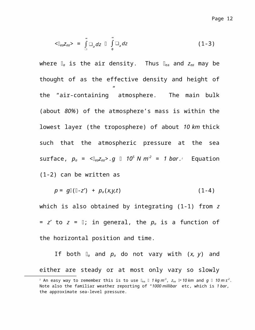
Figure 1-3. The ocean is treated as a (vertical) stack of thin layers each of thickness dz : shown are layers “1” and “2;” layer “0” is air. The Fmn is (shearing) force per unit (horizontal) area due to layer “m” on layer “n.” The formulae show that the net force per unit area in layer “1” is F1net = F01

+ F21 =dz.¶tzx/¶z. Therefore, the net shearing force per unit mass is F1net dx dy/(rdxdydz) = (¶tzx/¶z)/r. This, in the idealized case described in the text, is = ¶u/¶t, the acceleration in the x-direction.

For the so called Newtonian fluid such as water, the shear stress zx is

proportional to the vertical rate of change of fluid velocity (i.e. the vertical

“rate of strain”):

zx = ∂u∂ z (1-11)

where is the viscosity which to a good approximation may be taken as a

constant and moreover is rather small; it is 10-3 kg m-1 for water and

1.7×10-5 kg m-1 for air. Equation (1-11) is valid for laminar or slowly-

moving viscous flows void of turbulent movements we usually see in say, a

mountain stream or in swirling air vortices around a house. However, as

will be seen below, one often model oceanic and atmospheric flows using a

similar formula, except that an “eddy viscosity” e is used to represent the

aggregated effects of small eddies on the large-scale flows. The eddy

viscosity is much larger than the molecular viscosity and is moreover not a

constant – it depends on the flow. The “e” will be ascribed below but for

now we will proceed with our model formulation using equation (1-11).

Equation (1-9) then becomes:

∂u∂ t

= ∂∂ z

(❑e∂ u∂ z

) (1-12)

where e = e/, the kinematic eddy viscosity. This is a simple “heat-

diffusion” equation that can be easily solved subject to some initial

conditions and boundary conditions at z = 0 and z =H; for example:

u = 0, t = 0 (1-13)

u = 0, z = H (1-14a)

❑e∂u∂ z

=❑o

❑ , z = 0, (1-14b)

where to is a constant wind stress.

Exercise 1-1A : Use POM to solve (1-12) subject to (1-13) and (1-14) in a

periodic straight channel. Compare your solution with exact (analytical)

solution. Experiment with different grid sizes as well as with more

complicated initial and/or boundary conditions. Analyze and discuss your

results (e.g. use Matlab or IDL etc).

Exercise 1-1B : Repeat Exercise 1-1A using a e-profile that decays with

depth, e.g. e = eo exp(z), where eo and are constants.

Exercise 1-1C : Repeat Exercise 1-1A using an annulus channel (Figure 1-2)

instead of the straight (periodic) channel. Use a curvilinear grid (in POM)

for this exercise. Experiment with various values of Ranu and r. Compare

and discuss your results. Are the results substantially different from the

straight-channel case when Ranu is “not too large” (define what this means),

why? Is equation (1-12) still valid then? Why (or why not)?

1-2: Effects of Earth’s Rotation

In the above straight-channel flow example, we saw that the cross-

channel flow is nil. This is no longer true if the channel is placed on a

turntable and rotates about a vertical axis. We now expand the study of

wind-driven shearing flow to the case when the earth’s rotation cannot be

ignored. We can imagine that the earth is the “turntable.” If our channel is

placed at the (celestial) pole, then it rotates about the earth’s rotation axis

once every day (0.997258 day to be more exact) anticlockwise at the north

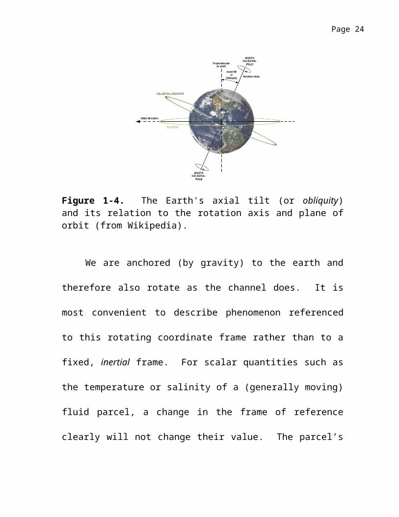
pole and clockwise at the south pole (Figure 1-4). Thus the rotational

frequency = 2/(86163.09 s) = 7.292 10-5 s-1. If the channel is placed on

the (celestial) equator, then there is no rotation (though the channel is being

carried west to east at a great speed = Rearth 1673 km/hour; Rearth 6371

km is the radius of a sphere having the same volume as the earth). At a

given latitude, the rotational frequency is:

Rot() = .sin(), /2 +/2 (1-15)

with the convention that positive (negative) is anticlockwise (clockwise).

Figure 1-4. The Earth's axial tilt (or obliquity) and its relation to the rotation axis and plane of orbit (from Wikipedia).

We are anchored (by gravity) to the earth and therefore also rotate as

the channel does. It is most convenient to describe phenomenon referenced

to this rotating coordinate frame rather than to a fixed, inertial frame. For

http://en.wikipedia.org/wiki/Orbital_plane_(astronomy)

http://en.wikipedia.org/wiki/Rotation

scalar quantities such as the temperature or salinity of a (generally moving)

fluid parcel, a change in the frame of reference clearly will not change their

value. The parcel’s momentum is a different story. While the phenomena

are still independent of the frame of reference, our perception of the

phenomena as well as their descriptions are altered. An example is offered

in Figure 1-5.

Figure 1-5. A turntable rotating at a constant radians/s with two observers “A” and “B” on it. At time t o “A” throws the ball (red) to “B.” A time-interval “Dt” later, the relative position of both observers are unchanged (and neither perceive any change). Let the ball’s speed be such that it arrives at the original B’s position in the same time-interval. To “A,” the ball has been forced to the right of “B.” This apparent force is called the Coriolis force. It is only perceived by “A” (and “B”) in the rotating frame but not felt by an outside observer in an inertial frame.

We now derive the momentum equation on a rotating frame. We

examine first the rate of change of an arbitrary vector (e.g. the momentum)

B = B1i1 + B2i2 + B3i3 in a rotating Cartesian frame of reference with unit

vectors (along x, y and z) i1, i2 and i3 [Pedlosky, 1979]. By chain rule:

( d Bdt )

I=

d Bk

dtik+

d ik

dtBk , (1-16)

where repeated index k means summation over all k = 1, 2 and 3, and the

subscript I denotes rates of change as seen from an observer in the inertial

frame, respectively. Clearly, the first term on the RHS of (1-16) is

( d Bdt )

R=

d Bk

dtik (1-17)

i.e. it is the rate of change of Bk when ik is fixed, i.e. when the observer is

himself rotating, hence is not able to sense the rotation of the coordinate

axes. The second term on the RHS of (1-16) involves d ik

dt , the rate of change

of a vector of fixed length (i.e. a unit vector), hence its change is completely

due to its changing direction as the coordinate axes rotate. From Figure 1-6,

we see that

( d Adt )=× A (1-18)

where is the angular velocity at which the constant-length vector A

rotates. Setting A = ik and using (1-17) and (1-18), equation (1-16) gives

( d Bdt )

I=( d B

dt )R+× B (1-19)

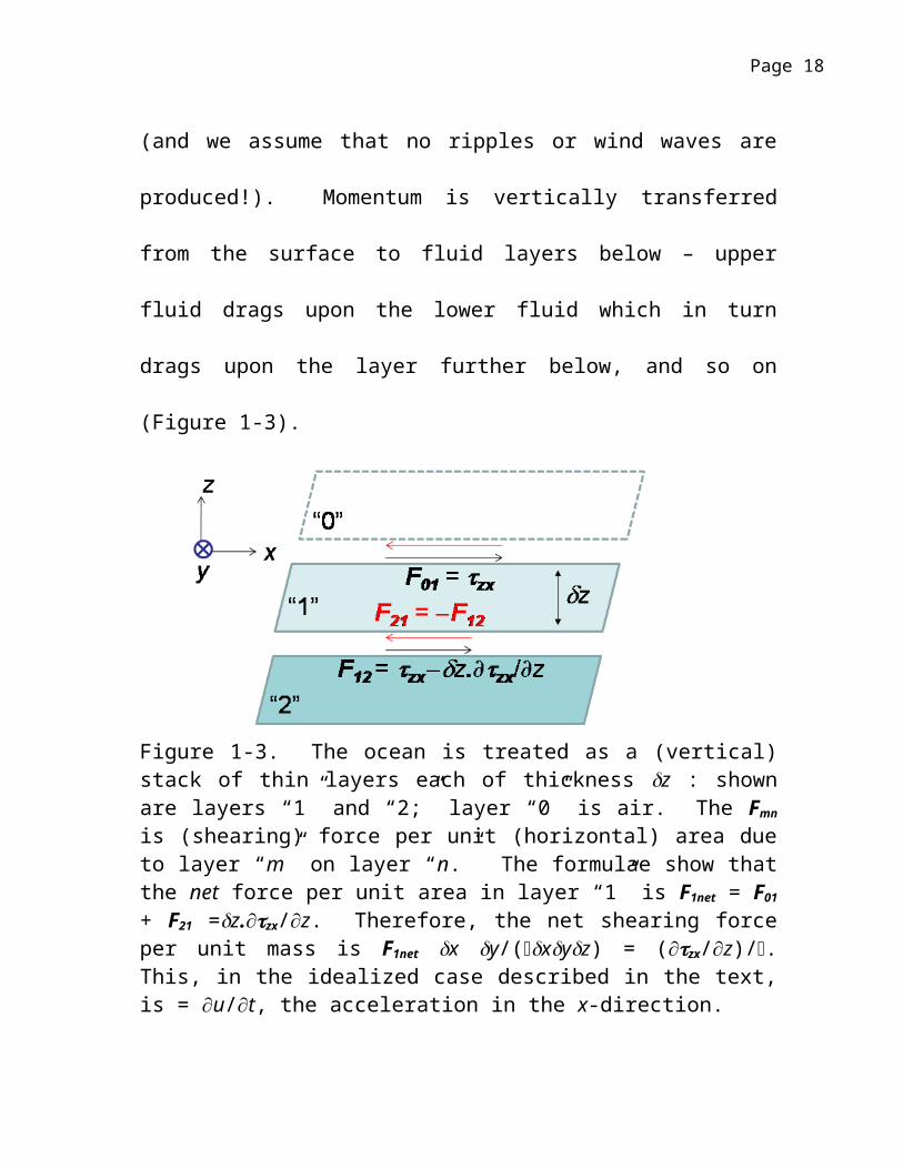
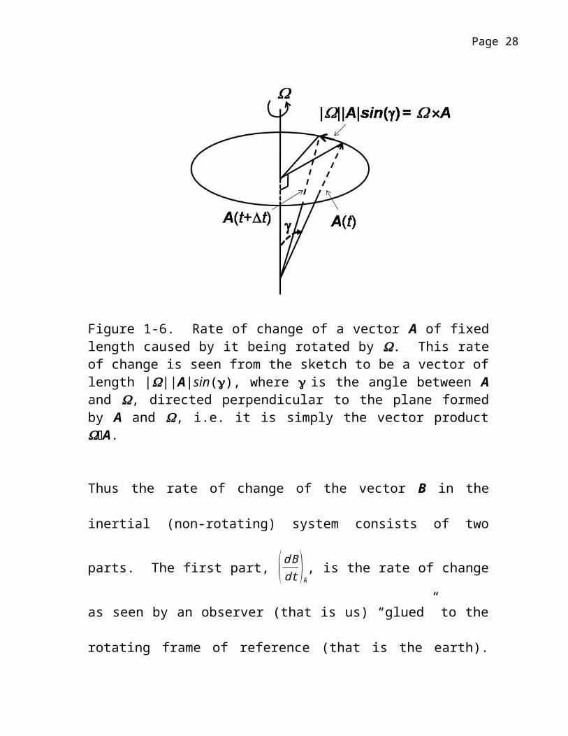
Figure 1-6. Rate of change of a vector A of fixed length caused by it being rotated by . This rate of change is seen from the sketch to be a vector of length |||A|sin(g), where g is the angle between A and , directed perpendicular to the plane formed by A and , i.e. it is simply the vector product A.

Thus the rate of change of the vector B in the inertial (non-rotating) system

consists of two parts. The first part, ( d Bdt )

R, is the rate of change as seen by

an observer (that is us) “glued” to the rotating frame of reference (that is the

earth). To this must be added the second part, B, in order that the correct

rate of change, ( d Bdt )

I, can be used in Newton’s law to describe fluid motion.

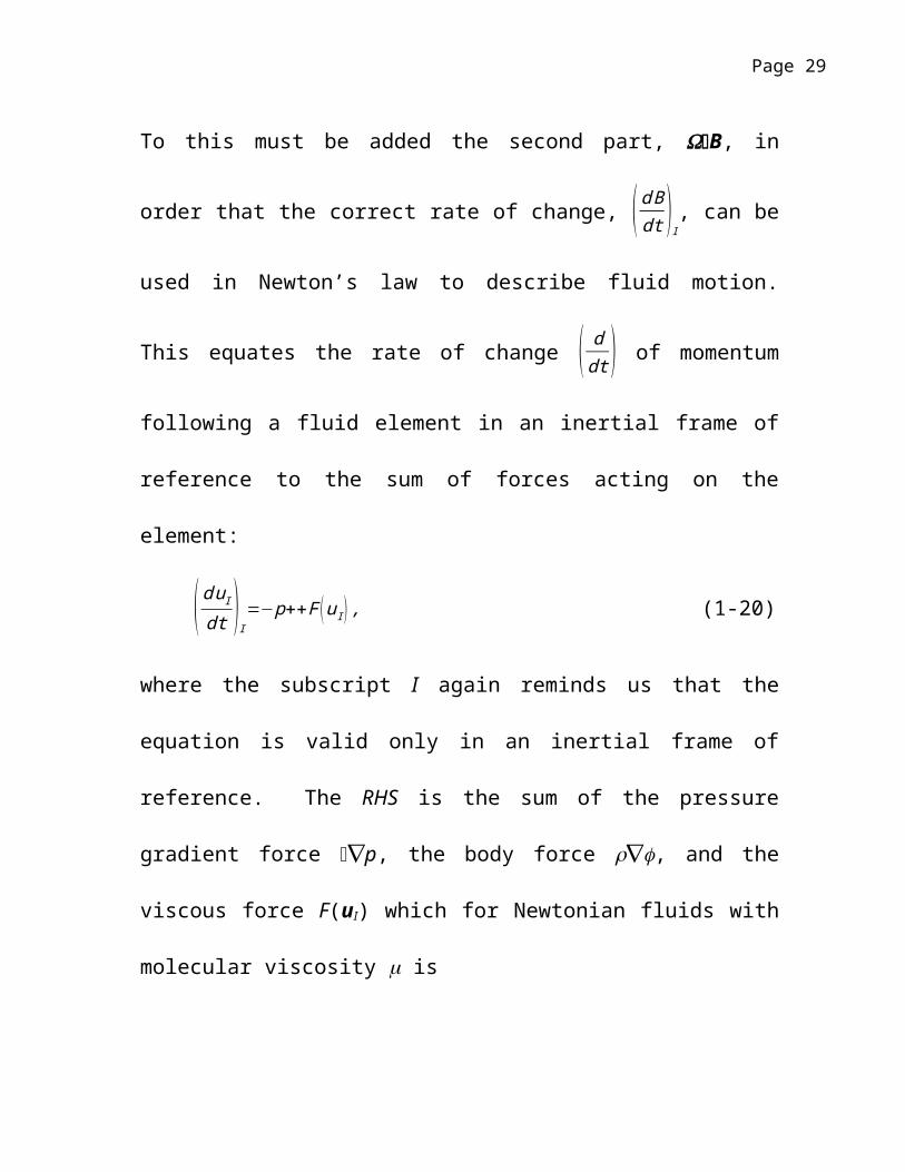
This equates the rate of change ( ddt ) of momentum following a fluid element

in an inertial frame of reference to the sum of forces acting on the element:

( d uI

dt )I=−p++F (u I ) , (1-20)

where the subscript I again reminds us that the equation is valid only in an

inertial frame of reference. The RHS is the sum of the pressure gradient

force p, the body force , and the viscous force F(uI) which for

Newtonian fluids with molecular viscosity is

F (u I )=(u I )+❑3 (uI ) . (1-21)

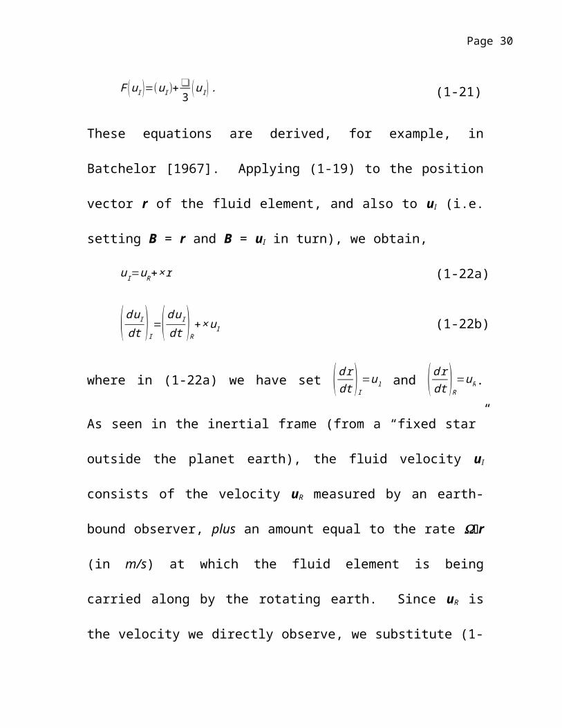
These equations are derived, for example, in Batchelor [1967]. Applying (1-

19) to the position vector r of the fluid element, and also to uI (i.e. setting B

= r and B = uI in turn), we obtain,

u I=uR+× r (1-22a)

( d uI

dt )I=( d u I

dt )R+×u I (1-22b)

where in (1-22a) we have set ( d rdt )I=u I and ( d r

dt )R=uR. As seen in the inertial

frame (from a “fixed star” outside the planet earth), the fluid velocity uI

consists of the velocity uR measured by an earth-bound observer, plus an

amount equal to the rate r (in m/s) at which the fluid element is being

carried along by the rotating earth. Since uR is the velocity we directly

observe, we substitute (1-22a) into (1-22b), (1-21) and (1-20) to express the

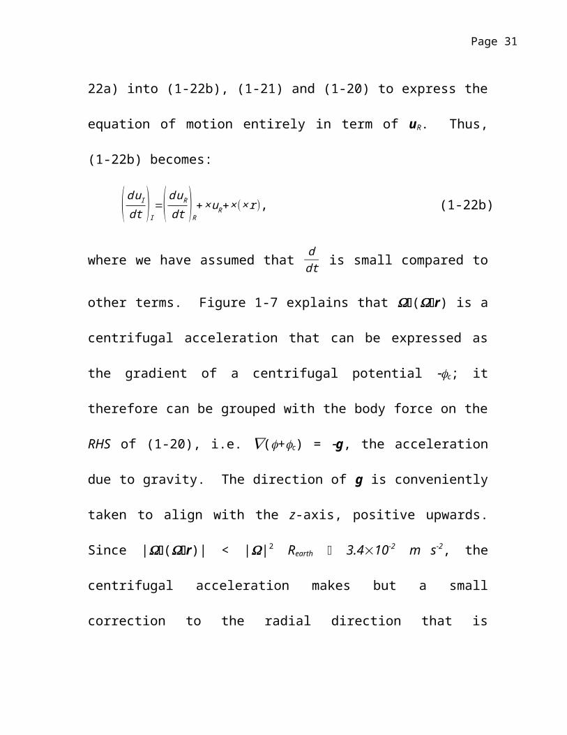
equation of motion entirely in term of uR. Thus, (1-22b) becomes:

( d uI

dt )I=( d uR

dt )R+× uR+×(× r ), (1-22b)

where we have assumed that ddt is small compared to other terms. Figure 1-

7 explains that (r) is a centrifugal acceleration that can be expressed as

the gradient of a centrifugal potential -c; it therefore can be grouped with

the body force on the RHS of (1-20), i.e. (+c) = -g, the acceleration due

to gravity. The direction of g is conveniently taken to align with the z-axis,

positive upwards. Since |(r)| < ||2 Rearth 3.410-2 m s-2, the

centrifugal acceleration makes but a small correction to the radial direction

that is “vertical” were the earth not rotating. Note that (r) is zero at the

poles and is maximum at the equator; it accounts for the slight bulge of the

earth around the equator. Substituting (1-22a) into (1-21), one can show that

F(uI) = F(uR). Thus substituting (1-22b) into (1-20) gives:

( d uR

dt )R=−×uR−p−g+F (uR ) , (1-23)

which is entirely in terms of quantities in the rotating frame of reference. As

written, equation (1-23) is valid also for non-constant . Henceforth the

subscript R will be dropped.

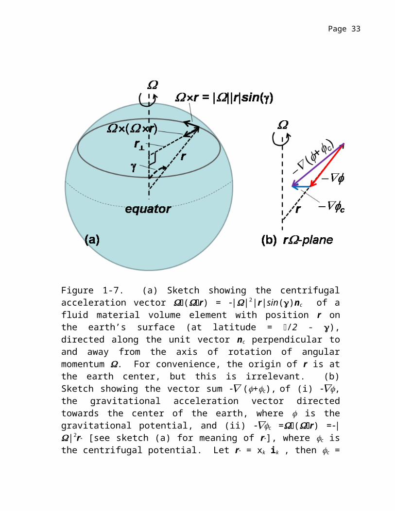
Figure 1-7. (a) Sketch showing the centrifugal acceleration vector (r) = -||2|r|sin(g)nc of a fluid material volume element with position r on the earth’s surface (at latitude = p/2 - g), directed along the unit vector nc

perpendicular to and away from the axis of rotation of angular momentum . For convenience, the origin of r is at the earth center, but this is irrelevant. (b) Sketch showing the vector sum - (+c), of (i) -, the gravitational acceleration vector directed towards the center of the earth, where is the gravitational potential, and (ii) -c =(r) =-||2r^ [see sketch (a) for meaning of r^], where c is the centrifugal potential. Let r^ = xk

ik , then c = (||2x2k )/2 as direct differentiation using = ik (¶/¶xk) shows.

Note also that c = (||2|r^|2)/2 = |r|2/2. In geophysics, the summed vector - (+c) = -g is called the acceleration due to gravity and the direction of g (i.e. “upwards”) is conveniently aligned with the z-axis.

The Equation of Motion Applied to Large-Scale Oceanic Flows :

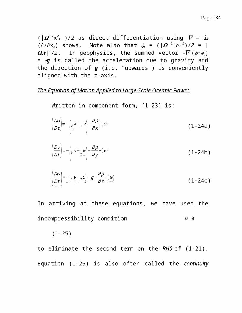
Written in component form, (1-23) is:

( DuDt )=−(2 w⏟−3 v)−

∂ p∂ x

+(u) (1-24a)

( DvDt )=−( 3u−1 w⏟)−

∂ p∂ y

+(v ) (1-24b)

( DwDt )⏟

=−(1 v−2u )⏟−g−∂ p∂ z

+(w)⏟ (1-24c)

In arriving at these equations, we have used the incompressibility condition

u=0 (1-25)

to eliminate the second term on the RHS of (1-21). Equation (1-25) is also

often called the continuity equation, a term that we will also use, though this

is correct only if effects of density change on mass balance are negligible.

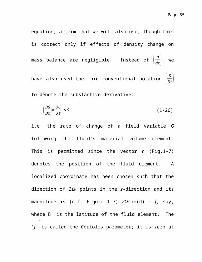
Instead of ( ddt ), we have also used the more conventional notation ( D

Dt ) to

denote the substantive derivative:

( DGDt )= ∂G

∂ t+uG (1-26)

i.e. the rate of change of a field variable G following the fluid’s material

volume element. This is permitted since the vector r (Fig.1-7) denotes the

position of the fluid element. A localized coordinate has been chosen such

that the direction of 23 points in the z-direction and its magnitude is (c.f.

Figure 1-7) 2sin() = f, say, where is the latitude of the fluid element.

The “f” is called the Coriolis parameter; it is zero at the equator, and is a

maximum (=2) at the pole as noted previously when discussing equation

(1-15). For large-scale, thin-fluid flows (i.e. D/L << 1) that we will mostly

focus on, it can be shown [e.g. Pedlosky, 1979; Gill, 1982] through a scaling

analysis that the (…)⏟ terms in (1-24) are generally quite small compared to

other terms in the same equation; these terms will therefore be dropped. The

molecular viscous terms (u) are also very, very small; though their

importance increases as the scale of motion becomes very small and

eventually they provide the necessary energy dissipation for the fluid

system. In models, effects of turbulence are usually parameterized by

invoking an eddy or effective viscosity which in the vertical (z) is denoted by

M (or diffusivity KH for heat and salt, chapter 3; two excellent texts are

Hinze, 1961, and Schlichting, 1963); these have much enhanced values than

their molecular counterparts: KM >> , a result of “eddy mixing” on the

small scales.3 Unlike the molecular viscosity, the eddy viscosity depends on

the flow itself, hence is a function of time and space, and in general takes

different forms in the vertical and horizontal directions (i.e. non-isotropic).

Various models of turbulence are available for KM (and KH). For example,

the Mellor and Yamada’s [1982] parameterization scheme is very popular

and is used in many oceanic and atmospheric circulation models including

the Princeton Ocean Model. While parameterizations for the vertical eddy

viscosity and diffusivity are relatively well-known, those for enhanced

horizontal eddy viscosity and diffusivity are in comparison still a subject of

much debate. Unless otherwise stated, we will assume that horizontal

viscosity and diffusivity are small, and include them only for the purpose of

numerical computations: stabilization of the numerical schemes and/or

elimination of grid-point (“2Dx” oscillatory) noise [e.g. Roach, 1972].

Excellent reviews of turbulence mixing in geophysical flows can be found in

the various chapters of the book edited by Baumert et al. [2005].

With the above simplifications, equation (1-24c) becomes

∂ p∂ z

=−g (1-27)

3 A proper treatment involves Reynolds averaging – see Hinze, 1961. Equation (1-24) is then called the Reynolds equation.

which is the hydrostatic equation (1-1) except that it is seen to be valid also

for non-uniform . Indeed, (1-24) admits a “static” solution

u = 0, = o(z) and p = po(z) (1-28)

which however is not very interesting. More interesting flows are produced

as a result of deviations of the pressure field from this hydrostatic state:

= o(z) + ’, p = po(z) + p’ (1-29)

where the ’ and p’ are perturbation density and pressure respectively. In

the ocean o oc = 1025 kg m-3 say, where oc is a constant density, and

’ is generally a small fraction of this: ’/o 0.01 and smaller. Subtracting

(1-28) from (1-24), letting o in the acceleration terms, and dividing

through by o, we obtain:

( DuDt )=+ fv− 1

❑o

∂ p '∂ x

+ ∂∂ z

(K M∂ u∂ z

) (1-30a)

( DvDt )=−fu− 1

❑o

∂ p '∂ y

+ ∂∂ z

(K M∂ v∂ z

) (1-30b)

∂ p '∂ z

=−' g (1-30c)

with an error in (1-30a,b) that is at most O(’/o).

1-3: Wind-Driven Homogeneous Flows with Rotation

Equations (1-25) and (1-30) are insufficient to solve for u, v, w, ’ and

p’. Additional equations involving the heat and salt equations as well as the

equation of state are required. These will be discussed in chapter 3. Here,

we study the case of a homogeneous fluid of constant density (i.e. ’ is

known, ’ = 0), for which equations (1-25) and (1-30) are then complete and

may be solved for u, v, w, and p’, given appropriate initial and boundary

conditions.

For this homogeneous fluid system, while ’ = 0, p’ is not and it may

be written in terms of the free surface . Assume then a free-surface z = (x,

t) in an idealized ocean of depth z = H but with no lateral boundaries.

There can be no flow across the surface and bottom, i.e. z = and z = H are

material surfaces, and D(z)/Dt and D(z+H)/Dt are both = 0:

w= ∂∂ t

+u ∂∂ x

+v ∂∂ y

,at z=( x , y , t ) , (1-31a)

w=−u ∂ H∂ x

−v ∂ H∂ y

,at z=−H ( x , y ) . (1-31b)

These equations constitute the upper and lower boundary conditions for our

problem. From (1-30c) with ’ = 0, we have p’ = p’(x, y, t); also the first of

(1-29) gives = o, a constant. Integrating (1-27) and using the second of

(1-29) yield:

p = ogz + function(x, y, t) = po(z) + p’(x, y, t), (1-32a)

from which we may let

po = ogz (1-32b)

Across the air-sea interface, z = , the total pressure p must be continuous

and equal to pa, so that (1-32) gives:

p’ = og + pa. (1-33)

The incompressibility condition (1-25) can now be used to relate (or p’) to

the velocity. Integrating (1-25) from z = H to z = and applying (1-31):

∂∂ t

=−∂ U∂ x

−∂V∂ y (1-34a)

(U ,V )=∫−H

❑

(u ,v ) dz (1-34b)

Equation (1-34) can also be re-written in term of a vertically-averaged

velocity (u , v )=∫−H

❑

(u , v ) dz /D, where D=H+¿, so that ∂∂ t

=−∂ Du∂ x

−∂ D v∂ y . The

form used in (1-34) shows explicitly however that the equation is valid for

general (u, v) that may also be a function of z (as well as of x, y and t).

Substituting (1-33) into (1-30a,b), the resulting equations and (1-34)

are grouped together here for convenience:

∂∂ t

=−∂ U∂ x

−∂V∂ y (1-35a)

( DuDt )=+ fv−g ∂

∂ x+ ∂

∂ z(K M

∂u∂ z

) (1-35b)

( DvDt )=−fu−g ∂

∂ y+ ∂

∂ z(K M

∂v∂z

). (1-35c)

These constitute three equations to be solved for (u, v, ) given appropriate

initial and boundary conditions. These are in fact the equations solved

numerically in POM. After (u, v) are solved, the incompressibility condition

(1-25) is then used to solve for w. Before we describe the numerical

solution however, it is instructive to examine more closely how one can

approach the problem analytically.

1.3.1 Boundary-Layer and Interior Flows :

For analytic treatment, we closely follow Pedlosky [1979]. We study

a problem in which the ocean is confined in the vertical by a free surface z =

(x,y,t) and a bottom z = H(x,y), but is unbounded in the horizontal. It is

more direct to use (1-25) and (1-30), which are repeated here:

∂ u∂ x

+ ∂ v∂ y⏟

(1)U /L

+ ∂ w∂ z⏟

(2 )W /D

=0 (1-36a)

∂ u∂ t

+u ∂u∂ x

+v ∂ u∂ y⏟

(1)U 2 /L

+ w ∂ u∂ z⏟

(2)WU /D

=+ fv⏟(3 )fU

− 1❑o

∂ p '∂ x⏟

(4)P/❑o L

+ ∂∂ z

(K M∂ u∂ z

)⏟

(5)KU /D2

(1-36b)

∂ v∂t

+u ∂ v∂ x

+v ∂ v∂ y⏟

(1)U 2 /L

+ w ∂ v∂ z⏟

(2)WU /D

=−fu⏟(3)fU

− 1❑o

∂ p '∂ y⏟

(4 )P /❑o L

+ ∂∂ z

(K M∂ v∂ z

)⏟

(5)KU /D 2

(1-36c)

∂ p '∂ z

=0 (1-36d)

Under each term, we indicate its order of magnitude by using the following

scale for each variable:

(x,y) L; z D; (u,v) U; KM K; (1-37a)

t L/U; w W ~ UD/L; (1-37b)

p’ P ~ oLfoU; f fo (1-37c)

where “” means “have/has the scale of.” Expression (1-37a) sets the basic

scales for the horizontal (L) and vertical (D) distances, and also the

horizontal velocity (U) and the eddy viscosity (K). The time scale (L/U) in

(1-37b) is chosen to be the “advective time scale,” i.e. the time taken for a

parcel of fluid to cover a distance of about L. For northern (southern)

hemisphere, f/fo = +()1. The vertical velocity scale W is chosen as follows.

In order to satisfy the continuity equation (1-36a), horizontal divergences or

convergences ( ∂ u∂ x

+ ∂ v∂ y ) must be balanced by vertical motion ∂ w

∂ z such that

their net sum is zero; thus we set terms (1) and (2) in (1-36a) to be of the

same order, and W ~ UD/L. It follows then that the scale of term (2) of

equations (1-36b,c), WU/D ~ U2/L, which is also the scale of term (1) of

these equations; although |w| is in general much smaller than |u| or |v|, it

multiplies the vertical gradient ∂u∂ z or ∂ v

∂ z which is generally much larger than

the horizontal velocity gradients such as u ∂ u∂ x . The scale for pressure in (1-

37c), P, is such that the horizontal pressure gradients balance the Coriolis

acceleration (see below). It is easy to see now that when the variables in (1-

36) are non-dimensionalized by the above scales, the equations become

[after dividing (1-36b,c) through by the scale (fU)]:

∂ u∂ x

+ ∂ v∂ y

+ ∂ w∂ z

=0 (1-38a)

( ∂ u∂ t

+u ∂ u∂ x

+v ∂ u∂ y

+w ∂ u∂ z )=v− 1

❑o

∂ p '∂ x

+Ev

2∂

∂ z(K M

∂ u∂ z

) (1-38b)

( ∂ v∂ t

+u ∂ v∂ x

+v ∂ v∂ y

+w ∂ v∂ z )=u− 1

❑o

∂ p '∂ y

+Ev

2∂

∂ z(K M

∂ v∂ z

) (1-38c)

∂ p '∂ z

=0 (1-38d)

where now all variables are dimensionless, and

¿ Uf o L

=Rossby number , Ev=2 K

f o D2=Ekman number (1-39)

are the two parameters of the problem (the factor “2” in Ev is for

convenience, below). The non-dimensionalized kinematic boundary

conditions at z = and z = H have the same form as equations (1-31a,b).

Equations (1-38b,c) show that the Coriolis and pressure gradient

terms are of the same order, both of these terms in (1-38b,c) are multiplied

by “1.” Thus by choosing the scales as those in (1-37c), we implicitly

assume that the Coriolis acceleration terms are important, and are in fact of

the same order of magnitude as the pressure-gradient terms. Clearly this

choice is only valid if “f” is not zero; the scaling (and balance of terms) will

need to be changed close to the equator. Observations of most oceanic (and

atmospheric) flows do indicate that away from the equator, pressure

gradients approximately balance Coriolis accelerations. From (1-38b,c) we

see that the conditions for this to be true are that the Rossby and Ekman

numbers are small. The former requires that either the flow is not strong

and/or the horizontal scale L is sufficiently large – for example, U 0.1 m/s,

L > 10 km for fo 10-4 s-1. The latter requires that the Ekman scale (2K/fo)1/2

is much smaller than the ocean depth D; if K 10-4~10-1 m2 s-1, this requires

that D > 10~50 m.

However, close to a boundary, no matter how small the eddy viscosity

KM is, at some point the shear terms Ev

2∂

∂ z(K M

∂(u , v)∂ z

) become important.

This is most apparent at the bottom boundary where the fluid parcel cannot

have a relative motion with respect to that boundary, i.e. the “no-slip”

condition must be satisfied:

ntu = 0, or approximately u = 0, at z = H(x,y) (1-40)

where nt is the unit vector tangential to the bottom. Therefore, unless the

flow is trivially zero, the interior (i.e. away from the bottom) velocity of a

real-fluid (i.e. fluid with viscosity) flow must decrease in value until it

becomes zero at the bottom.4 Since Ev is small, the only way the viscous

terms Ev

2∂

∂ z(K M

∂(u , v)∂ z

) can become large enough to balance the Coriolis

acceleration term is if the z-derivatives of (u, v) become very large, i.e. if the

decrease of velocity from the interior to the bottom occurs within a thin

layer in the immediate neighborhood of the bottom. This thin layer is called

a boundary layer, or a bottom boundary layer in the present case. A similar

thin layer also exists near the surface where wind stresses are applied.

Geostrophic Nearly-Inviscid Interior Flows:

Far away from boundaries, then, one expects that the flow is nearly

inviscid and one may approximate equation (1-38b,c) by dropping the term

4 An inviscid flow needs only to satisfy the no-normal flow condition equation (1-31b), so that a fluid parcel can ‘slip’ past the bottom.

involving Ev. Just exactly how far is “far” will be determined below. If is

also small, equations (1-38b,c) then give:

vg=1❑o

∂ p '∂ x (1-41a)

ug=1❑o

∂ p '∂ y (1-41b)

Oceanographers call the horizontal velocity (ug, vg) that satisfy (1-41)

geostrophic velocity, and the equation geostrophic relation. In the northern

hemisphere, a higher pressure in the south (east) than in the north (west),

¶p’/¶y < 0 (¶p’/¶x > 0) would produce an eastward (northward) geostrophic

velocity ug > 0 (vg > 0). The geostrophic flow around a center of high (low)

pressure is therefore clockwise (anticlockwise) or anticyclonic (cyclonic).

The direction of the flow is reversed in the southern hemisphere (f < 0). For

homogeneous fluid flow, since p’ is independent of z (see 1-38d), (ug, vg) is

therefore also independent of z. From (1-41), a geostrophic flow also has

zero horizontal divergence:

∂ug

∂ x+

∂ vg

∂ y=0, (1-42)

so that the corresponding vertical velocity wg satisfies:

∂ wg

∂ z=0 (1-43)

All three components of the geostrophic velocity (ug, vg, wg) are therefore

independent of z, the rotation axis. This is the Taylor-Proudman theorem

which is valid for inviscid homogeneous slow (small ) flow. If the upper or

lower boundary is flat, so that wg = 0 there, then wg = 0 through the water

column. The motion is then two dimensional, (ug, vg) 0, but wg = 0.

Figure 1-8 shows an example of this type of flow. (See Exercises).

Figure 1-8. Nearly-steady homogeneous (constant-density) flow in an x-periodic channel, 600km by 300km, of depth 200m except at the channel’s

center where a cylinder rises 50m above the bottom. Color is sea-surface height in meters and vectors are velocity at (A) z=0m (i.e. surface), (B) z=90m and (C) z=180m. This model calculation was carried out for 100 days when the flow has reached a nearly steady state. The experiment is meant to illustrate Taylor-Proudman theorem: flow below the cylinder’s height goes around the cylinder while above it the flow also tends to go around as if the cylinder extends to the surface. The velocity does not vary with “z” and the vertical velocity (which is not shown) is nearly zero.

Strictly speaking, the model solution in Fig.1-8 is still evolving in

time, so it is not steady and does not exactly satisfy equations (1-41), (1-42)

and (1-43). This is an important point – purely geostrophic flows satisfying

exactly (1-41) through (1-43) are indeterminate. Any p’(x,y) satisfies the

hydrostatic relation (1-38d), and (ug, vg) can be constructed to satisfy the two

(approximate) momentum equations (1-41a,b); the unknown (ug, vg) in turn

is horizontally non-divergent (equation 1-42) which simply requires that the

vertical velocity wg is independent of z. We know all these information

(hence the Taylor-Proudman theorem) but cannot pin down what the flow is!

To arrive at the unique model solution shown in Fig.1-8, we actually

included the small terms on the left hand side of momentum equations (1-

38b,c), the time-dependent terms in particular.5 Another way to pin down a

unique solution is to include the shear terms Ev

2∂

∂ z(K M

∂(u , v)∂ z

) which of

5 There were additionally horizontal viscous terms on the RHS of (1-38b,c) included for numerical stability, but these were small and unimportant to the arguments presented here.

course have the added benefit that we can then also satisfy the physically

relevant no-slip bottom condition (1-40) and the conditions at the sea surface

where windstress may be applied.

Viscous Boundary-Layer Flows:

It was mentioned before that no matter how small the Ekman number

Ev is, at some point close to the boundary the shear terms Ev

2∂

∂ z(K M

∂(u , v)∂ z

)

become large enough that they balance the Coriolis and pressure gradient

terms which by our scaling (see equation 1-38) are of O(1); purely

geostrophic flows then break down. Thus in a thin layer close to the

boundary, the small Ev multiplies ∂∂ z

(K M∂(u , v)

∂ z) to make their product O(1).

We express this mathematically by changing the coordinate z to , where

¿ zEv

1/ 2 (1-44)

so that the shear terms become

Ev

2∂

∂ z (K M∂ (u , v )

∂ z )=12

∂∂ (K M

∂ (u , v )∂ ), (1-45)

which is of O(1). The heuristic interpretation is, since ∂∂ z

(K M∂(u , v)

∂ z) is

large, of O(Ev-1), inside the boundary layer because a small change in z

results in a large change in (u, v), the change is made more gradual in the

stretched coordinate (i.e. ‘one moves more slowly’ in than in z) and one

can resolve or “see” the rapid velocity change so that the boundary condition

(1-40) (and a corresponding one at the surface, see below) can be satisfied.

The “z” measures distance changes outside the boundary layer, i.e. “z” is an

outer coordinate (see equation 1-37a, in which the dimensional z* (where

the asterisk denotes dimensional) is non-dimensionalized by the water depth

D >> boundary layer depth), and the geostrophic relation (1-41 through 1-

43) is an outer solution, though at the moment an incomplete one. Inside the

boundary layer, vertical distances are measured by scaled by a much

smaller (localized) length scale l* which from (1-44) is

l¿=D Ev1/2≪ D. (1-46)

The is called an inner coordinate, and the solution to be derived below is

called an inner solution. Indeed, equation (1-38) belongs to a class of

problems that are amendable to solution by the singular perturbation

methods, the early development and usage of which is in aerodynamics [van

Dyke, 1964].

With the new vertical scale l*, we have ∂ w∂ z

= 1Ev

1 /2∂ w∂ , which would

appear to be much larger than (and therefore cannot be balanced by) the

horizontal divergence term ∂ u∂ x

+ ∂ v∂ y in the continuity equation (1-38a). This

apparent dilemma is resolved by recognizing that in actuality the vertical

velocity w is very small. Indeed, inside the boundary layer, the continuity

equation requires that W*/l* ~ U/L, where W* is the scale of w inside the

boundary layer; thus

W ¿ l¿UL

=Ev1 /2 DU

L=Ev

1 /2 W (1-47)

where we have used (1-46) and (1-37b; for W). Therefore, because of the

thinness of the boundary layer, hence a much smaller aspect ratio l*/L than

the D/L previously assumed in (1-37), the appropriate vertical velocity scale

W* is correspondingly much smaller, by O(Ev1/2), than the scale W that we

have assumed. In the absence of other processes, the reader should satisfy

himself or herself to show that w* is the scale of the vertical velocity that is

valid both inside and outside the boundary layer.

If we now write the newly rescaled vertical velocity ~w as

~w = w*/W* = w.W/W* = w/Ev1/2 (1-48)

using (1-47), the w ∂∂ z terms on the RHS of the momentum equations (1-

38b,c) become:

w ∂(u , v)∂ z

=~w ∂(u , v)∂ (1-49)

and equation (1-38) becomes:

∂ u∂ x

+ ∂ v∂ y

+ ∂~w∂

=0 (1-50a)

( ∂ u∂ t

+u ∂ u∂ x

+v ∂ u∂ y

+~w ∂ u∂ )=v− 1

❑o

∂ p '∂ x

+ 12

∂∂ (KM

∂u∂ ) (1-50b)

( ∂ v∂ t

+u ∂ v∂ x

+v ∂ v∂ y

+~w ∂ v∂ )=u− 1

❑o

∂ p '∂ y

+ 12

∂∂ (K M

∂ v∂ ) (1-50c)

∂ p '∂

=0 (1-50d)

where (1-45) has been used in the viscous shear terms in (1-50b,c) and the

hydrostatic relation is unchanged but for a trivial change of the vertical

coordinate. Because of (1-50d) (or 1-38d), the thinness of the boundary

layer means that the pressure-gradient force (per unit mass), (¶p’/¶x,

¶p’/¶y)/o, may be represented by their values just outside the boundary

layer in the geostrophic interior of the water column, i.e., by (vg, ug) from

(1-41).

Now that equation (1-50) is properly scaled for flows inside the

boundary layer, we may simplify it (as we did with equation (1-38) when

deriving the geostrophic relation) by dropping the terms involving :

∂ u∂ x

+ ∂ v∂ y

+ ∂~w∂

=0 (1-51a)

0 ¿(v−vg)+12

∂∂ (K M

∂ u∂ ) (1-51b)

0 ¿(u−ug)+12

∂∂ (K M

∂ v∂ ) (1-51c)

where (1-41) has been used in (1-51b,c) to replace the pressure-gradient

terms by the geostrophic velocity. Also, the first (second) or top (bottom)

sign of or applies to the northern (southern) hemisphere with positive

(negative) Coriolis. Note that since (ug, vg) is independent of z (or ), the (u,

v) appearing in the -derivatives in equations (1-51b,c) may be replaced by

(uE, vE) = (u-ug, v-vg), (1-52)

the Ekman velocity; this is in fact what we will do below.

A wind stress is applied at the surface, and the boundary condition in

dimensional form is:

K M¿ ∂(u¿ , v¿)

∂ z¿=(X s

¿ ,Y s¿ ), at z* = 0 (1-54)

where the kinematic wind stress (Xs*, Ys

*) = (to*/o) (Xs, Ys), and to

* is the

scale of the wind stress in N m-2. In non-dimensional form, (1-54) is:

K M∂(u , v)

∂=α ( X s , Y s )=α τ s, at ζ = 0 (1-55a)

where ts = (Xs, Ys) is the non-dimensionalized kinematic wind stress, and

α=❑o

¿ D❑o UK Ev

1/2. (1-55b)

The boundary condition at the bottom is the no-slip condition:

(u, v) = (0, 0), at z = H (1-56)

Surface Boundary Layer with Constant Eddy Viscosity :

We assume constant eddy viscosity KM (= 1, non-dimensional), and

also that the depth of the channel is sufficiently deep that the surface and

bottom boundary layers do not interact. Equations (1-51b,c) are solved by

first re-writing them in terms of A = uE + ivE, where i = (1). Thus {(1-51c)

i (1-51b)} gives:

iA=12

∂2 A∂❑2 . (1-57)

We first consider the surface boundary layer, for which the solution that

satisfies (1-55a) and that vanishes as ~ (so that u ~ ug and v ~ vg as one

moves into the geoestrophic region outside the boundary layer) is:

uE+i vE=α2(1−i )(X s+ iY s)exp [(1 i)] (1-58)

or,

uE=αeζ

√2 [X s sin(ζ+ π4 )Y scos (ζ+ π

4 )] (1-59a)

vE=αeζ

√2 [X scos (ζ+ π4 )+Y ssin (ζ+ π

4 )] (1-59b)

In dimensional form, equation (1-59a,b) are:

uE¿= eζ

√K f o[X s

¿sin (ζ+ π4 )Y s

¿cos(ζ+ π4 )] (1-60a)

vE¿= eζ

√K f o[X s

¿ cos(ζ+ π4 )+Y s

¿sin(ζ+ π4 )] (1-60b)

where ¿ z¿/ (D E v1/2)=z¿ /√2 K / f o. Equation (1-59) shows that over a distance of

about

dE* = l* = √2 K / f o (1-61)

the velocity profiles (u, v) ~ (ug, vg), the geostrophic velocity in the ocean’s

interior outside the boundary layer. The dE* is called the Ekman depth; it

measures the thickness of the boundary layer which is therefore thicker for

larger K and/or smaller fo. At the surface, = 0, the vector product (uE, vE)

(Xs, Ys) gives the angle w between the velocity (uE, vE) and wind-stress

vector (Xs, Ys) as:

w = sin-1[cos(/4)] = /4; (1-62)

the positive (negative) sign is for the northern (southern) hemisphere and it

means that the Ekman velocity is directed to the right (left) of the wind

stress, at an angle of 45o.

To obtain w, we use the continuity equation (1-51a), and also (1-59):

−∂~w∂

=αeζ

√2 [ (∇ ∙ τ s ) sin (ζ+ π4 )k (∇× τ s)cos (ζ+ π

4 )] (1-63)

which gives upon integration ∫ζ

0

dζ ' and setting ~w ( x , y , 0 )=0:

~w ( x , y , ζ )=α2 [−eζ (∇ ∙ τ s ) sin ζ k (∇× τ s)(1−eζ cos ζ)] (1-64a)

In dimensional form, using equation (1-48), we have:

w ¿= 1f o

[−eζ (∇¿ ∙❑s¿) sin ζ k (∇¿×❑s

¿)(1−eζ cosζ )] (1-64b)

where = z*/(2K/fo)1/2.

Outside the surface boundary layer, ~ , the vertical velocity is:

~w ¿ (1-65)

In terms of the original variables “w” and “z,” we note from equation (1-44)

that the ~ means a finite but small z-distance below the surface, i.e.

~ is equivalent to z ~ 0 and Ev1/2 << 1, (1-66)

so that:

w ¿ (1-67a)

In dimensional form, this is:

w ¿¿ (1-67b)

Equation (1-67) is the main result from the analysis of surface boundary

layer: the effect of the wind is to induce a small vertical velocity which is

directly proportional to the wind stress curl:

k (∇× τ s )=∂ Y s

∂ x−

∂ X s

∂ y (1-68)

For positive wind stress curl, there is upwelling (downwelling) in the

northern (southern) hemisphere. The vertical velocity is small, but as we

shall see in a simple example, it has a profound effect on the interior flow

field. Before we give this example, it is necessary to conduct a similar

analysis on the bottom boundary layer near z =H.

Bottom Boundary Layer with Constant Eddy Viscosity :

The analysis for the bottom boundary layer follows much the same

way as for the surface layer. Instead of the wind-stress condition (1-55), we

now apply the no-slip condition (1-56). Let

zb = z + H (1-69)

where the subscript “b” (here and below) is used to denote the bottom

boundary layer, to distinguish the solution from that obtained previously for

the surface boundary layer. The bottom boundary layer is near zb > 0.

Equation (1-56) then becomes:

(u, v) = (0, 0), at zb = 0 (1-70)

The boundary-layer coordinate (1-44) becomes:

b=zb

Ev1 /2=

z+HEv

1/2 (1-71)

Equation (1-57) is the same, but a solution that decays as b ~ + is chosen:

uEb + i vEb = (ug + i vg) exp[(1 i)b ] (1-72)

which also satisfies the no-slip condition (1-70). Thus,

uEb=e−ζ b [−ugcos ζ b v gsin ζ b ] (1-73a)

vEb=e−ζb [± ug sin ζ b−v g cosζ b ] (1-73b)

and the corresponding dimensional form simply has the u’s and v’s replaced

by corresponding variables with asterisks:

uEB¿ =e−ζ b [−ug

¿ cosζ b v g¿ sin ζ b ] (1-74a)

vEB¿ =e−ζ b [± ug

¿ sin ζ b−vg¿ cosζ b ] (1-74b)

The vertical velocity is again obtained from the continuity equation (1-51a),

and also (1-73):

∂~wb

∂❑b=e−ζ b [k (∇×ug)sin ζ b ] (1-75)

which gives upon integration ∫0

ζ b

dζ ' and setting ~wb ( x , y , 0 )=0:

~w b (x , y , ζ b )=12 [1−e−ζ b(sin ζ b+cosζ b)] k (∇×ug) (1-76a)

In dimensional form, using equation (1-48), we have:

wb¿=√ K

2 f o[1−e−ζ b(sin ζ b+cos ζ b)]k (∇¿× ug

¿ ) (1-76b)

where b = (z*+H*)/(2K/fo)1/2.

In terms of the original variables “w” and “z,” we note from equation

(1-71) that the b ~ + means a finite but small z-distance above the bottom,

i.e.

b ~ + is equivalent to zb ~ 0+, or z = H+ and Ev1/2 << 1, (1-77)

so that (1-76a) and (1-48) give:

w ¿ (1-78a)

In dimensional form, this is:

w ¿¿ (1-78b)

Equation (1-78) is the main result from the analysis of bottom boundary

layer. Unlike the surface boundary layer, it is the interior geostrophic flow

that is driving the bottom boundary layer. In the northern (southern)

hemisphere, a positive curl in the geostrophic velocity produces upwelling.

A Simple Problem: Quasi-Geostrophic Interior Solution :

Equipped with the above boundary-layer formulae, we are now ready

to revisit the interior flow and attempt to close the otherwise indeterminate

(geostrophic) solution (equations 1-41 through 1-43). The correctly scaled

equation that governs the interior flow is (1-38). We will find an

approximate solution which as will become clear is called quasi-geostrophic.

We already saw that a first approximation is the geostrophic relation, and

indicated that the solution in Figure 1-8 was obtained through the inclusion

of small terms on the left-hand-side of the momentum equations. These

small terms represent small imbalances to the purely geostrophic relation.

Equations (1-38b,c) suggest then that the “degree” of this imbalance, or

ageostrophy, is of O(). It is reasonable to assume then that the solution

consists of predominantly the geostrophic part, plus a small correction that is

of O():

u = ug + u1 + O(2); v = vg + v1 + O(2); etc. (1-79)

and similarly for other variables also. Higher order correction terms , O(2)

and higher are also indicated in equation (1-79), since there is no reason to

expect that the geostrophic relation plus the O() correction (i.e. u1 etc) will

provide the complete solution. It is important to understand that just as the

(ug, vg, …) are properly scaled of O(1), the (u1, v1, …), (u2, v2, …), etc are

also all scaled to be of O(1). Only then it makes sense to assume the form of

(1-79) for (u, v, …). Equation (1-79) is called a perturbation expansion,

which by the way may not be necessarily convergent [van Dyke, 1964].

From the discussion prior to Figure 1-8 (Taylor-Proudman Theorem) the

geostrophic velocity components are all independent of z: ¶(ug,vg,wg)/¶z =

(0, 0, 0). In particular, for “w,” we already know from the boundary-layer

solutions at either the surface or the bottom boundary (see 1-67a and/or 1-

78a) that w ~ O(Ev1/2). Therefore, since Ev

1/2 << 1 ~ O() say, the

corresponding expansion (i.e. 1-79) for w = wg + w1 + … shows that

wg = 0, for all z; (1-80)

otherwise, the solution for w will be inconsistent with its small values near

the surface and bottom boundaries. In quasi-geostrophic approximations,

the vertical velocity component is very small, O(; Ev1/2), and represents only

the ageostrophic portion of the flow. However, this ageostrophy is very

important.

Substituting (1-79) into (1-38b,c), and collecting and equating terms

that are of O(1) and O() separately we obtain for the O(1) terms the

geostrophic relation as before, while the O() terms give:

∂u1

∂ x+

∂ v1

∂ y+

∂ w1

∂ z=0 (1-81a)

∂ug

∂ t+ug

∂ug

∂ x+v g

∂ug

∂ y=v1−

1❑o

∂ p1'

∂ x(1-81b)

∂ vg

∂ t+ug

∂ v g

∂ x+vg

∂ vg

∂ y=u1−

1❑o

∂ p1'

∂ y(1-81c)

∂ p1'

∂ z=0 (1-81d)

Note that the viscous terms Ev

2∂

∂ z¿ and the vertical advection terms

wg ∂(u¿¿ g , vg)

∂ z¿ are missing in (1-81) because ∂ (u¿¿ g , v g)

∂ z=(0,0)¿ of course,

but in the latter case also because wg = 0 from (1-80). Thus the O()

dynamics are also hydrostatic and incompressible, but are not in perfect

geostrophic balance. The ageostrophy is due to the unsteadiness and

advective terms by the geostrophic flow (i.e. the left-hand-side of 1-81b,c).

We eliminate the pressure gradients from (1-81) by subtracting the y-

derivative of (1-81b) from the x-derivative of (1-81c), i.e. by [¶(1-

81c)/¶x¶(1-81b)/¶y], and using (1-42) and also (1-81a):

∂❑g

∂ t+ug

∂❑g

∂x+v g

∂❑g

∂ y=f

∂ w1

∂ z (1-82)

where g = ¶vg/¶x¶ug/¶y is the relative vorticity of the geostrophic flow (not

to be confused with the scaled vertical coordinate of the boundary layer,

e.g. equations (1-44) or (1-71)). Since g is also independent of z, equation

(1-82) can be integrated ∫−H

0

dz to yield, upon using (1-67a) and (1-78a):

∂❑g

∂ t+ug

∂❑g

∂x+v g

∂❑g

∂ y=

f E v1 /2

H 2 ϵ [ α k (∇×τ s )−❑g ] (1-83)

Given the wind stress curl, ts, this equation now allows the

determination of the geostrophic vorticity field g, hence also the

geostrophic velocity (ug, vg). It is the consideration of the viscous boundary

layers near the surface (providing the wind stress curl) and also near the

bottom (providing the ‘damping’, g) that allows the existence of a small

vertical velocity and the determination of the O(1) geostrophic field. A

simple example further illustrates these ideas.

A simple problem:

Consider a homogeneous fluid in a channel of constant depth = H that

extends to in the x-direction; all fields (and forcing) are assumed

independent of the y-direction. A y-directed kinematic wind stress ts = (Xs,

Ys) is applied at the surface:

(Xs, Ys) = (0, x) (1-84a)

The solution is seeked only in the region L* x* +L*, where L* = 500 km,

or in terms of the non-dimensional “x,” in 1 x +1. Taking the scale of

the kinematic wind stress to*/o = 10-4 m2 s-2:

( X s¿ ,Y s

¿)=(0 ,10−4 ) x¿ /L¿m2 s−2; (1-84b)

we then have wind stresses of about 0.1 N m-2 at x* = 500 km. Since the

flow is independent of y, the geostrophic relation (1-41) requires that ug = 0.

Assuming also steady state, the LHS of equation (1-83) is then zero, yielding

the simple solution:

❑g=α k (∇×τ s ) (1-85a)

or in dimensional form:

(ug¿ , vg

¿ )=√ 2f o K ( X s

¿ ,Y s¿) (1-85b)

The solution (equation 1-85) states a simple balance between the applied

wind stress at the surface and the frictional damping dues to the viscous

effects at the bottom. Knowing the geostrophic velocity in the interior, the

complete solution is supplemented near the surface by equations (1-59) and

(1-64a) (or in dimensional forms, equations 1-60 and 1-64b) and near the

bottom by equations (1-73) and (1-76a) (or in dimensional forms, equations

1-74 and 1-76b). Some details of this solution are given in Figures 1-9 and

1-10 (see exercises).

Exercise 1-3A : Use POM to solve the simple problem (above) of wind-

driven flow in a channel. (See Figures 1-9 and 1-10). Modify the code to

solve also the case with no-slip conditions at the bottom, and replot the

figures for this latter case.

Exercise 1-3B : Use POM to solve the Taylor-Proudman column (Figure 1-

8). Note that in this case POM is modified without vertical viscosity. Solve

also the case of a seamount instead of the cylinder.

Exercise 1-3C : Use POM to solve a case that has wind as well as the

seamount: i.e. a combination of exercises 1-3A and 1-3B above. Derive the

corresponding analytical solution.

Figure 1-9. Nearly-steady homogeneous (constant-density) wind-driven rotational flow in a channel of depth 200m and theoretically unbounded in x, but in practice an x-length = 1000 km is used in the solution. The flow is assumed independent of y. The wind stress is specified in y-direction only: (0, 10-4).(x/500km - 1) m2 s-2. Panel (A) is for the y-directed velocity and

panel (B) the x-directed velocity. In (B), profiles of u are also plotted at the four indicated x-locations with scales 0.1 m/s given along the bottom for the first and fourth locations. Detailed plots comparing the profile at x=205 km (i.e. the first x-location) with analytical solution are given in Figure 1-10. The Coriolis parameter is constant, fo = 610-5 s-1, and the vertical eddy viscosity is also constant, K = 510-3 m2 s-1. This numerical solution is at time = 100 days, and differs slightly from the analytical one discussed in the text; instead of the no-slip condition at the bottom, a matching of the velocity to the law-of-the-wall log layer is used [see the POM manual by Mellor, 2004].

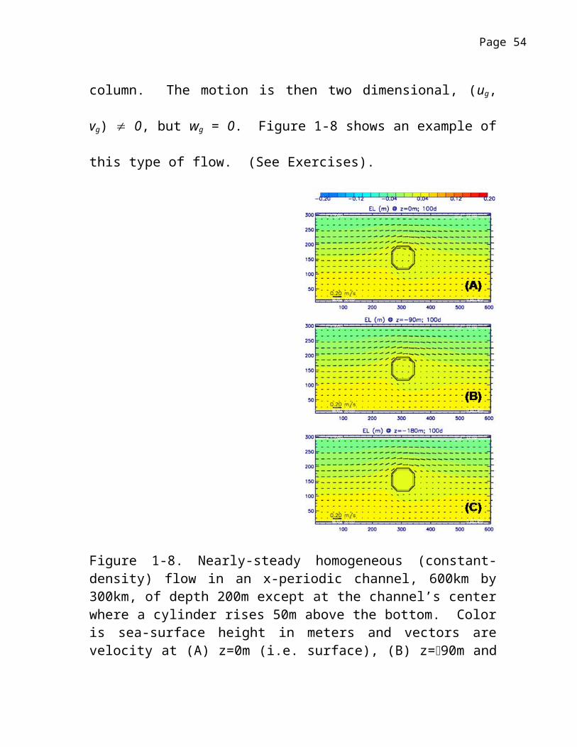
Figure 1-10. Profiles of (A) u, (B) v and (C) w at the x = 205 km location described in Figure 1-9b. Solid line indicates analytical solution assuming no-slip condition at the bottom, while dashed line the corresponding numerical (i.e. Figure 1-9) solution assuming log-layer at the bottom. Black line indicates the Ekman velocity while red (in panels (A) and (B)) indicates the total (Ekman + geostrophic) velocity. Note that in panel (B), total v/4 is plotted (so the profile fits in the same panel).

References

Batchelor, G.K., 1967: Fluid Dynamics.

Baumert et al., 2005:

Gill, A., 1982: Atmospheric & Oceanic Dynamics

Mellor, G.L., 2004: POM User Guide.

Mellor G.L. and Yamada, T., 1982: Review of Turbulence Models.

Pedlosky, J., 1979: Geophysical Fluid Dynamics.

Roach, P., 1972: Computational Fluid Dynamics.

Van Dyke, M., 1964: Perturbation Methods in Fluid Mechanics.

The potential temperature equation:

( DTDt )= ∂

∂ z(KH

∂T∂ z

)

The salinity equation:

( DSDt )= ∂

∂ z(K H

∂ S∂ z

)

The equation of state:

= (T, S, p)

Equations for turbulence mixing:

(KM, KH) = function(q2, q2l, stratification, shear, waves, …)

shoni2.princeton.edushoni2.princeton.edu/ftp/lyo/dpw/pom_v06.docx · web viewthis book is about...

Documents