vibration boundary control of micro-cantilever timoshenko

Scientia Iranica B (2018) 25(2), 711{720

Sharif University of TechnologyScientia Iranica

Transactions B: Mechanical Engineeringhttp://scientiairanica.sharif.edu

Vibration boundary control of micro-cantileverTimoshenko beam using piezoelectric actuators

A. Mehrvarza, H. Salarieha;�, A. Alastya, and R. Vatankhahb

a. School of Mechanical Engineering, Sharif University of Technology, Tehran, Iran.b. School of Mechanical Engineering, Shiraz University, Shiraz, Iran.

Received 27 April 2016; received in revised form 3 January 2017; accepted 17 April 2017

KEYWORDSTimoshenko microbeam;Piezoelectric actuator;PDE model;Boundary control.

Abstract. One of the methods of force/moment exertion on micro beams is utilizingpiezoelectric actuators. In this paper, considering the e�ects of the piezoelectric actuatoron asymptotic stability achievement, the boundary control problem for the vibration of aclamped-free micro-cantilever Timoshenko beam is addressed. To achieve this purpose, thedynamic equations of the beam actuated by a piezoelectric layer laminated on one side ofthe beam are extracted. The control law was implemented so that vibrations of the beamcould be decayed. This control law was achieved based on feedback of time derivatives ofboundary states of the beam. The obtained control was applied in the form of piezoelectricvoltage. To illustrate the impact of the proposed controller on the micro beam, the �nite-element method and Timoshenko beam element were used, and then simulation operationwas performed. The simulation shows that not only does this control voltage reduce thevibration of the beam, but also the mathematical proofs proposed in this article are preciseand implementable.© 2018 Sharif University of Technology. All rights reserved.

1. Introduction

Nowadays, micro systems are one of the most usefultools in science and technology that are given specialimportance and status. The main function of thesesystems is based on the deformation of a beam at microscale. Therefore, studying dynamic characteristics,behavior and control of the micro beams is of greatsigni�cance. For example, using micro beams inAtomic Force Microscopy (AFM) [1], micro switches,mass sensors, micro-accelerometers, micro mirrors, de-termining a suitable position for construction at microscale, Grating Light Valves (GLV) [2], can be noted.

For deforming micro beams, a suitable actuatoris required. Among the most common actuators, elec-

*. Corresponding author.E-mail address: [email protected] (H. Salarieh)

doi: 10.24200/sci.2017.4327

trostatic and piezoelectric actuators can be mentioned.Electrostatic actuators have so many applications suchas Grating Light Valves (GLV) [2]. Another commoncategory of actuators is piezoelectric actuators whichare used for micro beams excitation. These actuatorsare made of piezoelectric materials. One of the mostimportant properties of piezoelectric materials is theirdeformations caused by applying electric potential�eld. This property is used in piezoelectric actuators.In this method, a piezoelectric layer is attached to themicro beam. Since there is a constraint between thislayer and the micro beam, increasing the length of thepiezoelectric layer, due to applied voltage, will causebending and deformation on the beam [3]. This methodof stimulation is the basis of atomic force microscopyand is considered as the most e�ective tool in surfacetopography nowadays. The main application of thistool is the study of surface properties and manipulationof materials in nanoscale, surface modeling, assemblingnanoparticles, and their communication [4-6].

712 A. Mehrvarz et al./Scientia Iranica, Transactions B: Mechanical Engineering 25 (2018) 711{720

Many studies on modeling micro beams and theirassociated applications have been performed; GratingLight Valves modeling is one example in which themicro beam works by an electrostatic excitation [7],and micro pump modeling is another instance wherethe micro beam is used as a displacement creatoroperator [8].

Many studies have been done in the �eld of microsystems analysis which include the study of the idealmicro beam model behavior [9,10] and that of vibrationanalysis of beams [11,12].

In addition to the issues raised in the modelingand analysis of micro beams, there have been com-prehensive studies on control of beams. Based onthe application where the micro beam is used, thetarget for the control of micro beam may change. Forexample, if the beam is used as a micro switch, thetarget would be the position control of the end ofbeam [13]. Moreover, atomic force microscopy can beconsidered as another example. Since the set of atomicforce microscopy works in their resonant mode, thecontrol objective is vibration control of the beam intheir resonant mode [14]. Another important objectiveof control that is considerably signi�cant in the controlof micro beams is controlling the shape and positionof the beam. For example, this issue has particularimportance in the static atomic force microscopy [15].

Conventional control algorithms are usually suit-able for controlling systems that have Ordinary Dif-ferential Equations (ODE). Such algorithms are notappropriate for continuum systems, such as beams andmembranes. For this purpose, governing equationsshould be converted to ordinary di�erential equationsin the vibrational modes, and then they would becontrolled [3,16]. In contrast, in boundary controlalgorithm, the system is considered as a Partial Di�er-ential Equation (PDE) where the controller is appliedonto the boundary of the system and can changethe response by changing the boundary conditions ofthe system [17-19]. In this method, the boundaryparameters are changed in such a way that the desirablebehavior of the system is achieved eventually [20-25]. This method may have a variety of applicationsin industry since the system is actuated only byits boundary and the controller is used only by themeasured data from the boundary. For example, thismethod has been used to control the exible marineriser [26-28] and exible articulated wings on a RoboticAircraft [29].

In this paper, boundary control of a clamped-free micro-cantilever Timoshenko beam with the aimof vibration suppression is considered. The actuator isa piezoelectric layer attached to the beam. Consideringthe e�ects of piezoelectric actuator, a boundary controlis obtained which guarantees the asymptotic stabilityof the system. In this case, it is assumed that the

piezoelectric layer is ideally attached to the beam.In the second section, the dynamic equations of thesystem are derived. In the third section, a linearcontrol law based on the theory of boundary controlis constructed to suppress the system vibration. Inthe fourth section, Finite-Element Method (FEM) isutilized for modeling the system. Simulation resultsbefore and after applying the control law are presentedin the �fth section. Finally, conclusion is given in thelast section.

2. Model dynamics

A clamped-free micro-cantilever Timoshenko beam ispresented as the inspected beam to which a piezoelec-tric layer is ideally attached. hb is the beam thickness,hp is the piezoelectric thickness, L is the length ofbeam, and b is the width of beam, as shown in Figure 1.

Kinetic energy, T , and strain energy, U , of beamsare achieved by Eqs. (1) and (2):

T =12Ls0

�Avt2 + C�t2

�dx; (1)

U =12Ls0

�"33

bp

hpu2 � k1�xu�D�x2

�B(�x � �)2�dx: (2)

Partial di�erential equations of Timoshenko beam witha piezoelectric layer and boundary conditions obtainedfrom the Hamilton principle with a little modi�cationare given in [16]. A modi�cation is made to theequations, that is, no external force has been enteredinto the system. The resulting equations are as follows:(

A�tt �B (�xx � �x) = 0C�tt �D�xx �B (�x � �) = 0

(3)

8>>><>>>:� (0) = 0�x (1) = �k1

D u (t)� (0) = 0�x (1)� � (1) = 0

(4)

where x and t indicate the independent spatial and timevariables, respectively, �(x; t) represents the lateral

Figure 1. A schematic view of the beam withpiezoelectric actuator and some geometric parameters [16].

A. Mehrvarz et al./Scientia Iranica, Transactions B: Mechanical Engineering 25 (2018) 711{720 713

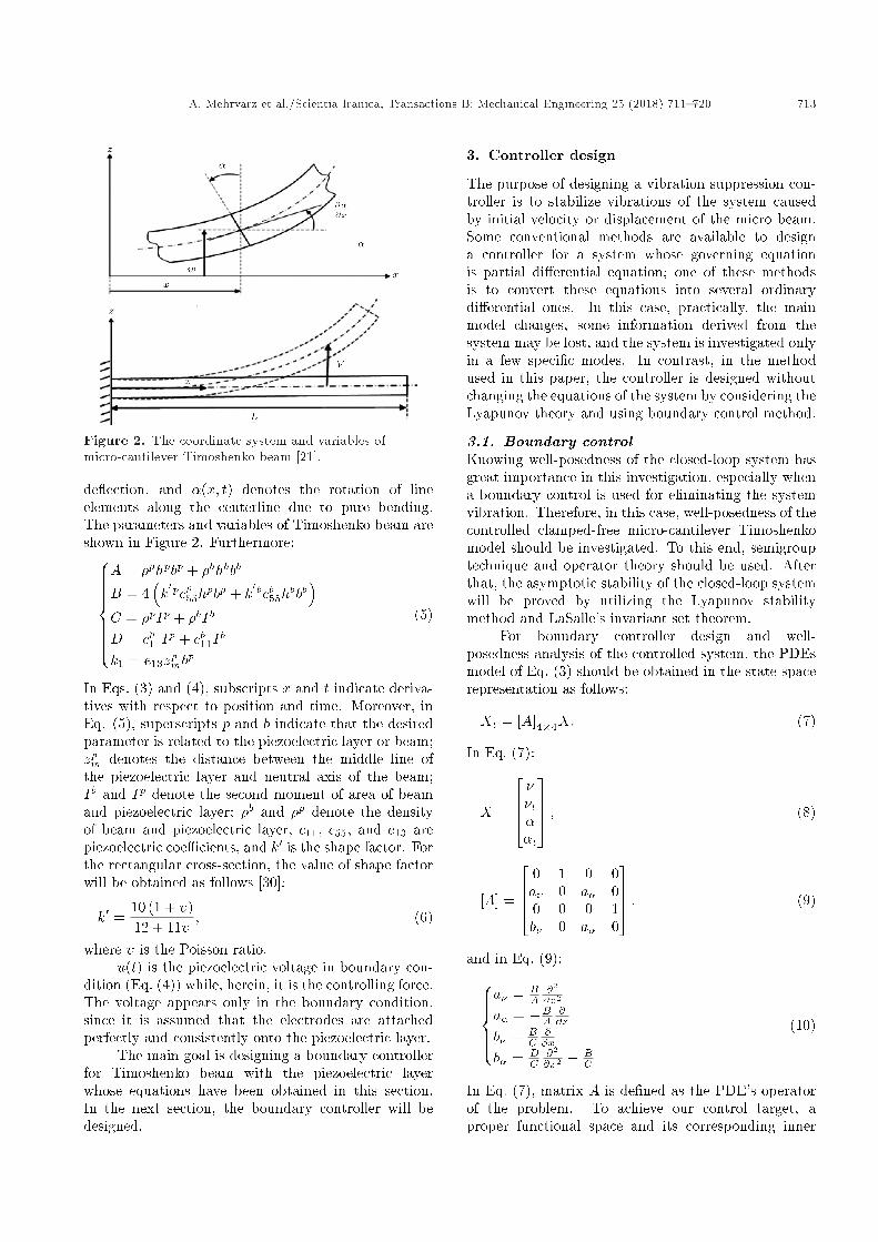
Figure 2. The coordinate system and variables ofmicro-cantilever Timoshenko beam [21].

de ection, and �(x; t) denotes the rotation of lineelements along the centerline due to pure bending.The parameters and variables of Timoshenko beam areshown in Figure 2. Furthermore:8>>>>>><>>>>>>:

A = �phpbp + �bhbbb

B = 4�k0pcp55hpbp + k

0bcb55hbbb�

C = �pIp + �bIb

D = cp11Ip + cb11Ib

k1 = e13zpmbp

(5)

In Eqs. (3) and (4), subscripts x and t indicate deriva-tives with respect to position and time. Moreover, inEq. (5), superscripts p and b indicate that the desiredparameter is related to the piezoelectric layer or beam;zpm denotes the distance between the middle line ofthe piezoelectric layer and neutral axis of the beam;Ib and Ip denote the second moment of area of beamand piezoelectric layer; �b and �p denote the densityof beam and piezoelectric layer, c11, c55, and e13 arepiezoelectric coe�cients, and k0 is the shape factor. Forthe rectangular cross-section, the value of shape factorwill be obtained as follows [30]:

k0 =10 (1 + �)12 + 11�

; (6)

where � is the Poisson ratio.u(t) is the piezoelectric voltage in boundary con-

dition (Eq. (4)) while, herein, it is the controlling force.The voltage appears only in the boundary condition,since it is assumed that the electrodes are attachedperfectly and consistently onto the piezoelectric layer.

The main goal is designing a boundary controllerfor Timoshenko beam with the piezoelectric layerwhose equations have been obtained in this section.In the next section, the boundary controller will bedesigned.

3. Controller design

The purpose of designing a vibration suppression con-troller is to stabilize vibrations of the system causedby initial velocity or displacement of the micro beam.Some conventional methods are available to designa controller for a system whose governing equationis partial di�erential equation; one of these methodsis to convert these equations into several ordinarydi�erential ones. In this case, practically, the mainmodel changes, some information derived from thesystem may be lost, and the system is investigated onlyin a few speci�c modes. In contrast, in the methodused in this paper, the controller is designed withoutchanging the equations of the system by considering theLyapunov theory and using boundary control method.

3.1. Boundary controlKnowing well-posedness of the closed-loop system hasgreat importance in this investigation, especially whena boundary control is used for eliminating the systemvibration. Therefore, in this case, well-posedness of thecontrolled clamped-free micro-cantilever Timoshenkomodel should be investigated. To this end, semigrouptechnique and operator theory should be used. Afterthat, the asymptotic stability of the closed-loop systemwill be proved by utilizing the Lyapunov stabilitymethod and LaSalle's invariant set theorem.

For boundary controller design and well-posedness analysis of the controlled system, the PDEsmodel of Eq. (3) should be obtained in the state-spacerepresentation as follows:

Xt = [A]4�4X: (7)

In Eq. (7):

X =

2664 ��t��t

3775 ; (8)

[A] =

2664 0 1 0 0a� 0 a� 00 0 0 1b� 0 a� 0

3775 ; (9)

and in Eq. (9):8>>><>>>:a� = B

A@2

@x2

a� = �BA @@x

b� = BC

@@x

b� = DC

@2

@x2 � BC

(10)

In Eq. (7), matrix A is de�ned as the PDE's operatorof the problem. To achieve our control target, aproper functional space and its corresponding inner


product should be de�ned due to the kinetic and strainenergies of the system represented in Eqs. (1) and (2).The appropriate functional space for our problem inoccupying region is chosen as follows:

V = H2()� L2()�H2()� L2();

where Lp() is a Lebesgue space (space of functionswith the property of [

R jf jpd�]

1p < 1); Hk()

is a Hilbert space that addresses Sobolev space,W k2(), of functions W k2() � Hk()ff : D�f 2L2(); for all 0 � � � kg, where D�:f is the �th-orderweak derivative of function f [31]. The correspondinginner product introduced in Hilbert space V has thefollowing form:

hY; Zi =12s

�Aa2b2 + Ca4b4 +Da3xb3x

+B (a1x � a3) (b1x � b3)�d; (11)

where Y = (a1; a2; a3; a4), Z = (b1; b2; b3; b4), and ai; bifor i = 1; 2; :::; 4 are scalar-valued functions de�ned on, where aj ; bj 2 H2(); j = 1; 3; aj ; bj 2 L2();j = 2; 4. Eq. (11) can be used to de�ne the mechanicalenergy of closed-loop system. The target of thisinvestigation is to show that System (3), with boundaryconditions of Eq. (4), which appeared in the followingequation under boundary feedbacks, is well-posed andhas an asymptotic decay rate:

u (t) = ku�t (L) : (12)

In Eq. (12), ku is the controller gain and has a positivevalue. This controller is applied to piezoelectric layeras voltage to reduce vibrations of Timoshenko microbeam.

The state space representation of the system inEqs. (3) and (4), under boundary controllers shown inEq. (12), is summarized as follows:8><>:Xt = [A]X

�0 : x = 0! � = �x = � = �x = 0�L : x=L! �x (L)=�k1

D u (t) ; �x (L)=� (L) (13)

Considering operator A and boundary conditions ofthe system in Eq. (13), the domain of operator A isdetermined as: D(A) = H4

�0() �H2() �H4

�0() �

H2() and:

H4�0

() =�f : f 2 H4 () ; f j�0 = fxj�0

: (14)

To illustrate well-posedness of the controlled systemexpressed in Eq. (13), �rst, it should be demonstratedthat operator A is a dissipative operator.

Theorem 3.1. Linear operator A, whose domain isde�ned in Eq. (14), is dissipative.

Proof. From the de�nition of the inner product inEq. (11), we have:

hX;XiV =12Ls0

�A�t2 + C�t2 +D�x2

+B(vx � �)2�dx = E (t) : (15)

The following result is achieved after applying thetime derivative to the above-mentioned positive de�-nite function which can be considered as a Lyapunovfunction:ddthX;Xi� =2hX;AXi� =

Ls0

�A�tt�t + C�t�tt

+D�x�xt +B (�x � �) (�xt � �t)�dx:(16)

By replacing �tt and �tt from Eq. (3), we have:

hX;AXi� =12Ls0

�B�t (�xx � �x)

+ �t�D�xx +B�x �B�

�+ +D�x�xt

+B�x�xt�B�x�t�B��xt+B��t�dx:(17)

With arranging Eq. (17), we have:

hX;AXi� =12Ls0

�B [(�t�xx + vx�xt) + (��x�t � ��xt)]

+D (�t�xx + �x�xt)�dx: (18)

Performing some integration by parts, the followingresults are achieved:

hX;AXi� =12

[B�t�x �B�t�+D�x�t] jL0 ; (19)

hX;AXi� =12

�B�t (L) �x (L)�B�t (0) �x (0)

�B�t (L)� (L) +B�t (0)� (0)

+D�x (L)�t (L)�D�x (0)�t (0)�:(20)

By applying the boundary conditions of Eq. (4), wehave:

hX;AXi� = �12k1�t (L)u (t) : (21)

Finally, by applying boundary control laws of Eq. (12),the following result can be obtained:


hX;AXi� = �12k1ku�t2 (L) : (22)

According to Eq. (22), it is concluded that hX;AXiV �0 for the closed-loop system of Eq. (13). Thus, fromthe de�nition of the dissipative operators [32], the proofwill be completed.�

Theorem 3.2. The operator ( I � A)�1 exists andis continuous for any > 0.

Proof. We consider the following equation:

( I�A)X = X0: (23)

For demonstrating the existence of the operator ( I �A)�1, it is su�cient to show that there is only onesolution to Eq. (23). By applying the result ofTheorem 3.1 illustrated in Eq. (22), we have:

h( I �A)X;XiV = h X;AXiV � hAX;XiV= hX;XiV +

12k1ku�t2 (L)

� hX;XiV = kXk2V : (24)

With the above result, it is concluded that the bilinearform a with the de�nition of a(u; �) = h( I�A)u; vi iscoercive on the Hilbert space, V . Now, using the Lax-Milgram theorem, one can easily prove that Eq. (23)has a unique weak solution, and so the operator ( I �A)�1 exists [33,34].

It is shown that the operator ( I � A)�1 isbounded and, as given in [31], it will be continuous.Thus, in order to complete the proof, it is su�cientto show that the operator ( I � A)�1 is bounded. Asshown, Inequality (24) is attained from the dissipativityof operator A. Now, one can conclude that:

kXk2V � h( I �A)X;XiV = hX0; Xi� kX0kV kXkV ! kX0kV � kXkV : (25)

So, jjXjjV is bounded when jjX0jjV is bounded and theproof is completed.�

Theorem 3.3. The set of Eq. (13), with the initialcondition X(t = 0) 2 D(A), is well-posed.

Proof. Since the closure of function space, D(A), isH4() � H2() � H4() � H2() � V , it is clearthat D(A) is dense in V . It is evidential that rangeof ( I � A), R( I � A) = V is dense in V . Also,according to Theorem 3.2, ( I � A) has a continuousinverse ( I�A)�1 for any > 0. Therefore, accordingto the de�nition of resolving the set of an operator [32], is in the resolving set of operator A.

As shown in Theorem 3.1, it is demonstrated thatoperator A is a dissipative operator. Therefore, basedon the Lumer-Phillips theorem [34], the system pre-sented in Eq. (13), containing the boundary controllersof Eq. (12), with any initial condition X(t = 0) 2D(A), is well-posed.�

The asymptotic stability of the closed-loop systemis achieved using LaSalle's invariant set theorem, whichis based on the Lyapunov method. For this target, �rst,it is required to show that the operator ( I � A)�1 iscompact for any > 0 [35].

Theorem 3.4. The operator ( I � A)�1 is compactfor any > 0.

Proof. It should be proved that the operator ( I �A)�1 is bounded for any > 0 [32]. This subject isshown in the proof of Theorem 3.2. Also, it is obviousthat:

( I �A)�1V 2 D (A) = D (A) : (26)

Since the closure of ( I �A)�1V is H4()�H2()�H4()�H2() and this space is compactly embeddedin H2()� L2()�H2()� L2() [32], according toRellich-Kondrachov compact embedding theorem [32],the compactness of the above-mentioned resolving setis obtained and the proof will be completed.�

Now, the proof of the asymptotic stability ofthe closed-loop system using LaSalle's invariant settheorem would be performed.

Theorem 3.5. The states of the closed-loop systemof Eq. (13) with the boundary feedback control laws ofEq. (12) will tend asymptotically toward zero.

Proof. We introduce the following Lyapunov func-tional candidate, which is the mechanical energy of theclosed-loop system, E(t) = hX;XiV � 0. As shown inthe proof of Theorem 3.1, time derivative of the abovefunctional is derived as:

_E (t) = �k1ku�t2 (L) ; (27)

where the superimposed dot indicates di�erentiationwith respect to time t. One can easily see fromEq. (27) that _E(t) � 0. Accordingly, function E(t)admits the requirements of a Lyapunov function. Atthis step, because of the compactness of resolving( I�A)�1 proved in Theorem 3.4, the LaSalle invariantset theorem [35] gives the asymptotic decay rate of thecontrolled states, and the proof will be completed.�

In this section, stability of the Timoshenko beamwith piezoelectric layer has been proved. Mathematicalproof is su�cient for showing the asymptotic stabilityof the proposed controlled system. However, numericalsimulation has been presented to show the accuracyand applicability of the proposed method.


4. Finite-element model

This section discusses the issue of modeling the beamby considering the Timoshenko beam element. It isassumed that the element has two nodes, and each nodehas the following variables:

[� �]:

� and � have the following polynomial forms:(v = c1 + c2x� = c3 + c4x

(28)

Eq. (28) can be written in a matrix form as in Eq. (29):

��

�=�1 x 0 00 0 1 x

�2664c1c2c3c4

3775 = gC = gh�1q

= g

26641 0 0 00 0 1 01 Le 0 00 0 1 Le

3775�1 2664�1

�1�2�2

3775 = Nq: (29)

For obtaining constant parameters ci, i = 1; :::; 4; hmatrix in two points x = 0; Le is de�ned. In addition,Le indicates the length of the beam element.

In Eq. (29), N is the shape function and will bede�ned as in Eq. (30):

N=gh�1=�H1 0 H2 00 H1 0 H2

�: (30)

Hi, i = 1; 2; is de�ned as in Eq. (31):(H1 = 1� x

LeH2 = x

Le

(31)

By using kinetic and strain energy of Systems (1) and(2), and variational method [36], the mass, sti�ness,and force matrices will be obtained as in Eqs. (32)-(34),respectively:

Ke =Les0

(B1TDB1 +B2

TBB2)dx; (32)

Me =Les0

(D1TAD1 +D2

TCD2)dx; (33)

Fe =Les0�1

2k1UBT1 dx: (34)

As a result, Di and Bi; i = 1; 2, are:

8>>>>>>>>>>>>><>>>>>>>>>>>>>:

B1 =h0 @

@x

iN

B2 =h@@x �1

iN

D1 =h1 0

iN

D2 =h0 1

iN

(35)

By replacing and integrating matrices, Eqs. (36)-(38)will be obtained as follows:

Ke =

26666666664

BLe

B2 � B

LeB2

B2

DLe + BLe

3 �B2 BLe6 � D

Le

� BLe �B2 B

Le �B2B2

BLe6 � D

Le �B2 DLe + BLe

3

37777777775; (36)

Me =

2666666666666664

ALe 0 ALe 0

3 CLe 6 CLe

0 3 0 6ALe 0 ALe 0

6 CLe 3 CLe

0 6 0 3

3777777777777775; (37)

Fe =

26666666640

k1U2

0

�k1U2

3777777775 : (38)

Here, we assume that ten nodes for our system andmatrices M , K, and F will be obtained by assemblingthe matrices given by Eqs. (36)-(38). Time evolutionof the system will be obtained by numerical integrationof Eq. (39) as follows:

[M ] f�qg+ [K] fqg = fFg : (39)

5. Simulation

In this section, the simulation operation with regardto System (1) has been performed with boundarycondition in Eq. (2). A proper control gain obtainedfrom trial and error which has a suitable settling


Table 1. Material properties of silicon dioxide for beam and PZT for actuator.

MaterialSiO2 PZT

Density (�) (kg/m3) 2200 7700Poisson coe�cient (�) 0.17 0.31

Young modulus of elasticity (E) (GPa) 73 71Piezoelectric constants (10-12 C/N) { d31 = 175

d33 = 400d55 = 580

Relative permittivity 3.9 1700

time and transient response is considered as ku = 0:2.It should be mentioned that by increasing the valueof controller gain, vibrations of the beam decreaserapidly; however, it causes numerical problems dueto sti�ness of equations and severe slopes in velocityand displacement variables, which a�ect the simulationresults. Indeed, ku = 0:2 is the most suitable gain,which can be utilized in our simulations without anynumerical di�culty. A silicon dioxide micro cantileverwith a PZT layer laminated on one of its side isconsidered as a case study. The physical characteristicsof the beam and piezoelectric layer can be found inTable 1 [2,16,37]. According to Table 1:

e13 =3X1

d3ic1i = �3:621 C/m2: (40)

The geometry of the piezoelectric layer and beam isgiven in Table 2 [16].

Using the following de�nitions of parameters, the

Table 2. Geometrical dimensions of beam andpiezoelectric layer (all in �m).

Beam length (L) 90Beam thickness (hb) 10

Beam width (bb) 30Piezoelectric thickness (hp) 10

Piezoelectric width (bp) 30

governing equation of the system will become non-dimensionalized:8>>>>>>><>>>>>>>:

~x = xL ~�b = �b

�b ~e13 = e13e13

~L = LL ~�p = �p

�b ~c1 = c1�bL2!1

~b = bL

~Ib = IbL4 ~c2 = c2

�bL2!1ehp = hpL

~Ip = IpL4 ~u = ue13

�bL3!21

~hb = hbL ~cij = cij

�bL2!21

~t = t!1

(41)

Considering that there are ten nodes in the beam andutilizing the information available in Tables 1 and 2, 40ordinary di�erential equations should be numericallysolved at the same time. At �rst, it is assumed that noforce enters to the system, and in Eq. (39), F matrixis set to zero. The micro beam behavior is shownin Figure 3. Then, it is assumed that the systemis closed loop, and there is controlling force on thebeam obtained from the piezo-electric actuator. Thebehavior is shown in Figure 4. The control signal isused as the piezoelectric voltage shown in Figure 5.

As it is clear, after applying the control action,vibrations of the system are suppressed and the systembecomes asymptotically stable.

6. Conclusion

In this paper, the governing partial di�erential equa-tions and corresponding boundary conditions of micro-

Figure 3. Open-loop response of the micro beam: (a) Lateral de ection �(x; t) and (b) rotation of line elements along thecenterline �(x; t).


Figure 4. Closed-loop response of the micro beam: (a) Lateral de ection �(x; t) and (b) rotation of line elements alongthe centerline �(x; t).

Figure 5. Control voltage u(t) = ku�t(L).

cantilever Timoshenko beams were obtained. Trans-verse vibration of the micro beam was stabilized bydesigning proper boundary control laws. This controllaw was achieved from the feedback of time deriva-tives of boundary states of the beam. The obtainedcontrol was applied in the form of voltage of thepiezoelectric actuator. Boundary stabilization wasinvestigated using the Lyapunov stability method andLaSalle's invariant set theorem. To demonstrate theperformance of the designed controllers via numericalsimulation, the �nite-element method was used tosimulate the open-loop and closed-loop systems. In theFEM, the Timoshenko beam element was used. At theend, computer simulation results veri�ed the achievedtheoretical results of this work.

References

1. Inderm�uhle, P., Sch�urmann, G., Racine, G., and DeRooij, N. \Atomic force microscopy using cantileverswith integrated tips and piezoelectric layers for actu-ation and detection", Journal of Micromechanics andMicroengineering, 7(3), p. 218 (1997).

2. Maluf, N. and Williams, K., Introduction to Micro-electromechanical Systems Engineering, Artech House(2004).

3. Zhang, W., Meng, G., and Li, H. \Adaptive vibrationcontrol of micro-cantilever beam with piezoelectricactuator in MEMS", The International Journal ofAdvanced Manufacturing Technology, 28(3-4), pp. 321-327 (2006).

4. G�ahlin, R. and Jacobson, S. \A novel method to mapand quantify wear on a micro-scale", Wear, 222(2),pp. 93-102 (1998).

5. Garc��a, R., Calleja, M., and P�erez-Murano, F. \Localoxidation of silicon surfaces by dynamic force mi-croscopy: Nanofabrication and water bridge forma-tion", Applied Physics Letters, 72(18), pp. 2295-2297(1998).

6. Miyahara, K., Nagashima, N., Ohmura, T., andMatsuoka, S. \Evaluation of mechanical propertiesin nanometer scale using AFM-based nanoindentationtester", Nanostructured Materials, 12(5), pp. 1049-1052 (1999).

7. Furlani, E. \Simulation of grating light valves", inTechnical Proceeding of the 1998 International Con-ference on Modeling and Simulation of Microsystems(1998).

8. Arik, M., Zurn, S., Bar-Cohen, A., Nam, Y., Markus,D., and Polla, D. \Development of CAD model forMEMS micropumps", in Technical Proceedings of the1999 International Conference on Modeling and Sim-ulation of Microsystems (1999).

9. Bernstein, D., Guidotti, P., and Pelesko, J. \Mathe-matical analysis of an electrostatically actuated MEMSdevice", Proceedings of the Modeling and Simulation ofMicrosystems MSM, pp. 489-492 (2000).

10. Liu, J., Mei, Y., Xia, R., and Zhu, W. \Largedisplacement of a static bending nanowire with surfacee�ects", Physica E: Low-Dimensional Systems andNanostructures, 44(10), pp. 2050-2055 (2012).

11. Alhazza, K.A., Daqaq, M.F., Nayfeh, A.H., andInman, D.J. \Non-linear vibrations of parametri-cally excited cantilever beams subjected to non-linear


delayed-feedback control", International Journal ofNon-Linear Mechanics, 43(8), pp. 801-812 (2008).

12. Zhao, D., Liu, J., and Wang, L. \Nonlinear freevibration of a cantilever nanobeam with surface e�ects:Semi-analytical solutions", International Journal ofMechanical Sciences, 113, pp. 184-195 (2016).

13. McCarthy, B., Adams, G.G., McGruer, N.E., and Pot-ter, D. \A dynamic model, including contact bounce,of an electrostatically actuated microswitch", Journalof, Microelectromechanical Systems, 11(3), pp. 276-283(2002).

14. Jalili, N. and Laxminarayana, K. \A review of atomicforce microscopy imaging systems: application tomolecular metrology and biological sciences", Mecha-tronics, 14(8), pp. 907-945 (2004).

15. Krstic, M., Guo, B.-Z., Balogh, A., and Smyshlyaev,A. \Control of a tip-force destabilized shear beam byobserver-based boundary feedback", SIAM Journal onControl and Optimization, 47(2), pp. 553-574 (2008).

16. Shirazi, M.J., Salarieh, H., Alasty, A., and Shabani, R.\Tip tracking control of a micro-cantilever Timoshenkobeam via piezoelectric actuator", Journal of Vibrationand Control, 19(10), pp. 1561-1574 (2013).

17. Canbolat, H., Dawson, D., Rahn, C., and Vedagarbha,P. \Boundary control of a cantilevered exible beamwith point-mass dynamics at the free end", Mecha-tronics, 8(2), pp. 163-186 (1998).

18. Dogan, M. and Morgul, O. \Boundary control of a ro-tating shear beam with observer feedback", Journal ofVibration and Control, 18(14), pp. 2257-2265 (2011).

19. Fard, M. and Sagatun, S. \Exponential stabilization ofa transversely vibrating beam via boundary control",Journal of Sound and Vibration, 240(4), pp. 613-622(2001).

20. Sadek, I., Kucuk, I., Zeini, E., and Adali, S. \Optimalboundary control of dynamics responses of piezo actu-ating micro-beams", Applied Mathematical Modelling,33(8), pp. 3343-3353 (2009).

21. Vatankhah, R., Naja�, A., Salarieh, H., and Alasty, A.\Asymptotic decay rate of non-classical strain gradientTimoshenko micro-cantilevers by boundary feedback",Journal of Mechanical Science and Technology, 28(2),pp. 627-635 (2014).

22. He, W., Ge, S.S., How, B.V.E., Choo, Y.S., and Hong,K.-S. \Robust adaptive boundary control of a exiblemarine riser with vessel dynamics", Automatica, 47(4),pp. 722-732 (2011).

23. Yang, K.-J., Hong, K.-S., and Matsuno, F. \Boundarycontrol of a translating tensioned beam with varyingspeed", Mechatronics, IEEE/ASME Transactions on,10(5), pp. 594-597 (2005).

24. Vatankhah, R., Naja�, A., Salarieh, H., and Alasty,A. \Boundary stabilization of non-classical micro-scalebeams", Applied Mathematical Modelling, 37(20), pp.8709-8724 (2013).

25. Vatankhah, R., Naja�, A., Salarieh, H., and Alasty,A. \Exact boundary controllability of vibrating non-classical Euler-Bernoulli micro-scale beams", Journalof Mathematical Analysis and Applications, 418(2),pp. 985-997 (2014).

26. He, W., Ge, S.S., and Zhang, S. \Adaptive boundarycontrol of a exible marine installation system", Auto-matica, 47(12), pp. 2728-2734 (2011).

27. How, B., Ge, S., and Choo, Y. \Active control of ex-ible marine risers", Journal of Sound and Vibration,320(4), pp. 758-776 (2009).

28. Nguyen, T., Do, K.D., and Pan, J. \Boundary controlof coupled nonlinear three dimensional marine risers",Journal of Marine Science and Application, 12(1), pp.72-88 (2013).

29. Paranjape, A.A., Guan, J., Chung, S.-J., and Krstic,M. \PDE boundary control for exible articulatedwings on a robotic aircraft", Robotics, IEEE Trans-actions on, 29(3), pp. 625-640 (2013).

30. Han, S.M., Benaroya, H., and Wei, T. \Dynamics oftransversely vibrating beams using four engineeringtheories", Journal of Sound and Vibration, 225(5), pp.935-988 (1999).

31. Reddy, J.N., Applied Functional Analysis and Varia-tional Methods in Engineering, McGraw-Hill College(1986).

32. Robinson, J.C., In�nite-Dimensional Dynamical Sys-tems: An Introduction to Dissipative Parabolic PDEsand the Theory of Global Attractors, 28, CambridgeUniversity Press (2001).

33. Yosida, K., Functional Analysis, Springer (1980).

34. Pazy, A., Semigroups of Linear Operators and Appli-cations to Partial Di�erential Equations, 44, SpringerNew York (1983).

35. Guo, B.-Z. and Morg�ul, �O., Stability and Stabilizationof In�nite Dimensional Systems with Applications,Springer Science & Business Media (1999).

36. Huebner, K.H., Dewhirst, D.L., Smith, D.E., and By-rom, T.G., The Finite Element Method for Engineers,John Wiley & Sons (2008).

37. Gad-el-Hak, M., MEMS: Introduction and Fundamen-tals, CRC press (2005).

Biographies

Amin Mehrvarz received his BSc and MSc degreesboth in Mechanical Engineering from Sharif Universityof Technology (SUT), Tehran, Iran in 2013 and 2015,respectively. His current research interests includenonlinear systems and control, PDE control, specialpurpose robotics and intelligent machines, vibration


analysis and control of distributed parameter systemsand vehicle control.

Hassan Salarieh received his BSc degree in Mechani-cal Engineering and also Pure Mathematics from SharifUniversity of Technology, Tehran, Iran in 2002. Hegraduated from the same university with MSc and PhDdegrees in Mechanical Engineering in 2004 and 2008.At present, he is an Associate Professor in MechanicalEngineering at Sharif University of Technology. His�elds of research are dynamical systems, control theory,and stochastic systems.

Aria Alasty received his BS and MS degrees in Me-chanical Engineering from Sharif University of Technol-ogy (SUT), Tehran, Iran in 1987 and 1989, respectively,and his PhD degree in Mechanical Engineering fromCarleton University, Ottawa, Canada in 1996. Atpresent, he is a Professor of Mechanical Engineering

at SUT. He has been a member of the Center ofExcellence in Design, Robotics, and Automation (CE-DRA) since 2001. His main areas of research includenonlinear and chaotic systems control, computationalnano/micro mechanics and control, special-purposerobotics, robotic swarm control, and fuzzy systemcontrol.

Ramin Vatankhah received his BS degree in Mechan-ical Engineering from the Shiraz University, Shiraz,Iran in 2007. He received his MS and PhD degreesin Mechanical Engineering from the Sharif Universityof Technology, Tehran, Iran in 2009 and 2013. Heis currently an Assistant Professor of the Departmentof Mechanical Engineering at Shiraz University. Hisresearch interests include nonlinear vibration, chaoscontrol, evolutionary computation techniques, bound-ary control of partial di�erential equations, nonlinearcontrol, and fuzzy system control.

vibration boundary control of micro-cantilever timoshenko

Documents