Error estimation in target height finding using VHF radar and three-antenna system positioned one above the other

Hristo Kabakchiev, Ivan Garvanov, Vladimir Kyovtorov

Institute of Information Technologies��������,

1113, Sofia “Acad. G. Bontchev” str., bg. 2

e-mail: ckabakchiev@iit.bas.bg, igarvanov@iit.bas.bg vladimir_ak@yahoo.com

Abstract: In the present paper the target elevation error is estimated. VHF radar and a three-

antenna positioned one above the other is used. The sensitivity of the elevation finding algorithm versus the coefficient of reflection, variation of input signal amplitude and phase is studied. Mean square error of elevation estimation versus target range and elevation is obtained.

1. Introduction. VHF radars are used for target range azimuth estimation. Using some

additional receiving antennas and signal processing allows performing of target elevation estimation [1, 2, 4]. If the elevation is known, the target height could be evaluated. The elevation estimation strongly impacts on the target height measuring. That the target range is great in the surveying radars small inaccuracies in elevation finding could lead into big errors in target height finding. Using this method, the accuracy of elevation estimation depends on the antennas number and the relief in the beam reflection point. The interval of elevation estimation depends on the number of antennas. The more antennas are the large interval of elevation measuring is. Despite the improving the elevation finding parameters, increasing the antennas number is not practical expedient. Therefore, this paper concerns VHF radar having three-antenna system arranged one above the other.

The method that we investigate uses the information resulting from the interference between the direct target signal and ground reflected target signal [1] fig.1. The used principles of elevation measurement are described in [1, 2, 4].

The interference picture of the electromagnetic field in the three antennas point (1, 2 and 3) is studied. As a result, the elevation (�) could be measured [1]. The assumption that the interference picture consists of only superposition between direct and reflected beam is used. For an instance, point 2 includes the signals R0,2 and R1,2 fig.1. Only the elevation (�) changing has an influence over the interference in these points. An amplitude comparison of the three signal level makes the elevation measurement accurate [1]. The amplitude comparison has ambiguity in the elevation measuring. Therefore, a suitable phase method is used for removing the ambiguity. The algorithm consists of two main parts "phase comparison" and " amplitude comparison" [1]. The phase comparison is used for roughly estimation the interval of elevation. A three bit coding is used [1]. The structure of this code simply describes the interval of elevation. The refinement of the elevation needs an error signal, which can be obtained by the amplitude comparison among the signals in the three antennas. A different error signal is used for different elevation interval. The estimated amplitude difference is compared with � previously estimated error signal versus the elevation and mapped into a pattern. As a result, the elevation could be obtained. During the study a simplified model of earth model is used [1,2].

2

Fig. 1 Diagram of VHF radar using three antenna system positioned one above the other

2. Target height estimation The target height can be evaluated through the following, well known, mathematical

dependence. βtgRHT 0= (1)

where 0R is the range to the target projection on the earth, β is the elevation fig.1 . This equation shows the target height could be precisely obtained through accurate

estimation the target range and elevation. The range 0R could be measured comparatively accurate, therefore the main investigations in this paper concern only the elevation estimation.

Mathematical dependencies between the target ranges and the target height shown in fig.1 The each range from each antenna to the target could be expressed as:

( ) 3,2,1220,0 =−+= iHHRR iTi (2)

The reflected ray travels another way (shown in fig.1) that could be expressed accordingly:

( ) 3,2,1220,1 =++= iHHRR iTi (3)

3. An algorithm for elevation estimation using VHF radar having antenna array

situated one above the other. The resulting interfering signal in each antenna could be expressed as [1]:

( ) 3,2,12

exp.2

exp ,1,0 =��

���

�−Γ+��

���

�−= iRjRjU iii λπ

λπβ (4)

where ( )rr jϕρ exp=Γ is the ground reflection coefficient. For horizontal polarization and smooth surface = -1( πϕ =r 1=rρ [1,2]. These expressions consider a simplified model of the ground surface which is characterized only by the reflection coefficient. Graphics of the three interfering signals ( )()(,)( 321 βββ U�UU ) having a ground refdlection coefficient =1 are shown in fig.2. The results are obtained in radar antennas height 4m, 7m, 12m and transceiver frequency 180MHz.

�� �

H1

H3

H2

O3

O2

O1

R0,3

R0,1

R0,2

R1,2

R�,2 R0

B2

�

HT

3

The three heights of the antennas could be configured in different way in order to changing the mutual arrangement of the interfering signal (crests and the falling) [1]. Two stages are used in the elevation measurement:

- A roughly estimation - A fine estimation

3.1 A roughly estimation of the elevation interval. This stage consists of estimation interval of elevation through three-bit coding the phase

difference in the signals. For example, the phase angle detection equation between the )(1 βU and )(2 βU is:

( )( ) ( )( )ββφ 212,1 UangleUangle −= (5)

( )[ ] ( )( )�

�

<≥

==Φ0cos,00cos,1

cos2,1

2,12,12,1 φ

φφsign (6)

After phase estimation between three interfering signals a three bit coding is made in order

to find roughly the interval of elevation tab.1.

Tab. 1 Elevation interval

12Φ 13Φ 23Φ Elevation interval

1 1 1 0.50 ÷ 40 1 0 0 40 ÷ 6.60 0 0 1 6.60 ÷ 80 0 1 0 80 ÷ 120

Fig. 2 the interfering signal in the three antennas and phase differences between each other versus elevation.

4

3.2 A fine elevation estimation; After roughly finding the elevation interval the fine elevation estimation is performed. For

this purpose an error signal is used. It is a product of the amplitude comparison of the three interfering signals in the three antennas. As a result three different values could be obtained

)()(),( 3,23,12,1 βββ �and�� :

( ) ( ) ( )( ) ( )ββ

βββ

21

212,1 UU

UUE

+−

=

( ) ( ) ( )( ) ( )ββ

βββ

31

313,1 UU

UUE

+−

=

( ) ( ) ( )( ) ( )ββ

βββ

32

323,2 UU

UUE

+−

=

(7)

Fig.3 shows the error signal curves ( )()(),( 3,23,12,1 βββ �and�� ) versus the elevation. It

can be seen that they have different gradient and hold a fluctuating behavior that could lead to ambiguity of elevation estimation. This ambiguity could be eliminate through the roughly estimation of the elevation interval.

Each interval of elevation has some different error curves that could be used for fine elevation estimation. For example, in the interval 0.50 ÷ 40 all curves )()(),( 3,23,12,1 βββ �and�� could be used without possibility appearance of ambiguity. It is preferable curves with height gradient to be used, because the error of estimation is less. According to the example with interval 0.50 ÷ 40 this curve is �1,3.

The mechanism of elevation finding consists of a comparison the obtained signal error

amplitude with previously estimated and tabulated error signal – the pattern. The difference between the measured and the previously tabulated errors is a consequence of the changing:

- The ground reflection coefficient (the roughness variation [2,4]); - inconsistence of the amplitudes and phases in the analogue receivers (front-end devices);

Fig. 3 The error curves according the equation 7.

5

- Signal to noise ratio at the analogue receivers input; There are an another way of estimating the error signal when the signal from two antennas is

considered only (U1 and U2)[1]:

( ) ( ) ( )[ ]( ) 2

1

2*1

2,1

.Re

ββββ

U

UUE = (8)

In this case the curve E 1,2 has low gradient [1]. Therefore, this method is not considered in this paper.

The error in elevation finding could come from several factors: (1) the relief surface, (2) the inconsistence of phases and amplitudes in the three front-end channels, (3) signal to noise ratio in the three front-end channels

The influence of the earth surface: In the literature four situations of the earth surface are considered [1]: (I) A smooth flat

surface; (II) A flat surface with roughness; (III) A sloped flat surface; (IV) A sloped flat surface with roughness. In the situations (I) and (II), the reflecting point lies on a horizontal line. If the mean value of the relief height h is zero and the standard deviation is hσ , therefore the mean ground reflectance from the earth surface is:

( ) ( )ψψρρ 2220

2220 sin.sin2exp hkIhkr −= , (9)

Where 0ρ is the reflectance of smooth surface and 10 =ρ ; λπ2=� , λ is the radio wave length;

22hh σ= ; ψ - is the angle of incidence of the radio wave; I0(.)- is a Bessel function in order zero.

The reflecting coefficient from the earth surface (4) depends on the mean value of the ground reflectance (9).

The roughness is defined as λψσ /)sin( hD = [1,4]. Fig.4 shows the roughness versus the

reflection. If we consider roughness D=0.05, the reflection coefficient will be rρ =0.82.

If we have the situations (III) and (IV), a correction of the phase pattern should be made

according to the equation.:

( )22

202,1 2 hHHRR T ∆+++= , (10)

Fig.4 Roughness versus ground reflection coefficient

6

If the point of ground reflection to the first antenna is a point of departure, the mean height that increases the reflected point to the second antenna is h∆ (fig.5). According to [1] if the h∆ =1m a 0.4� elevation error is possible. Eliminating this error is possible through correction the signal level estimation or preliminary recalculating the pattern versus the condition of working the radar in, as the value. During the pattern computing according to (7) the Ri,j should be considered according to (7) [1] .

Inconsistence of phases ad amplitudes in the three channels. It is known that the front-end devices are analogue therefore the fully consistence is hardly

doable. This inconsistence makes parasite amplitude and phase modulation in each analogue channel. If the relative amplitude and phase inconsistencies between antenna 1 and antenna 2 is A and ϕ , the total interfering signal is:

( ) ( ) ( ) �

� �

���

���

�−Γ+��

���

�−+= 2,12,02

4exp.

4expexp1 RjRjjAU

λπ

λπϕβ (11)

Considering the mean square error of A and ϕ are correspondingly ϕσσ andA the mean square elevation error is shown at fig.9.

4. Simulation results 4.1 A preliminary geometric analysis

The purpose of the preliminary geometric analysis is finding some geometrical characteristics and the opportunities of practical using.

earth

H1

H3

H2

O3

O2

O1

R0,3

R0,1

R0,2

R1,2

R�,2 R0

B2

�

HT

h∆

Fig.5 Diagram of VHF radar with three-antenna array system working in a condition of slope surface.

7

Fig.6 dependency of U3 versus the changing

target range for different elevations Fig.7 dependency of U3 versus the changing

target range ( 0 – 150m ) for different elevations

Fig. 6 and fig.7 show graphics of the U3 signal behavior versus the target range in different elevations. The other signals (U1, U2) behavior is analogous to the U3 – typical curve variations are observed in the beginning 0 – 150m and then the signals constant character (150m �� 300km). As a result, we can draw the conclusion that the signal levels in the inputs of the three antennas don't depend on the target range for ranges more than 150m. This independence is a prerequisite for the accurate elevation estimation. Therefore, accurate elevation estimation could be performed after target range more than 150m. Practically if is fully acceptable.

Fig.8 shows the distance of the reflection point from the radar (RB,I fig.1)versus target height and different active antenna heights . The range from the radar to the point of beam reflection can be expressed as:

iT

iTTiB HH

HHRHiR

+−−

=22

,

)(,

(12)

HT – is the target height; Hi- the height of active radar antenna ; RT – target range (the range between Hi and the target) The greater the target range and the lower the antenna is, the longer the distance to the reflection point is. This fact can be considered in the following earth reflection

Fig. 8 point of reflection versus target height for different target ranges and different height of the active radar

antenna

8

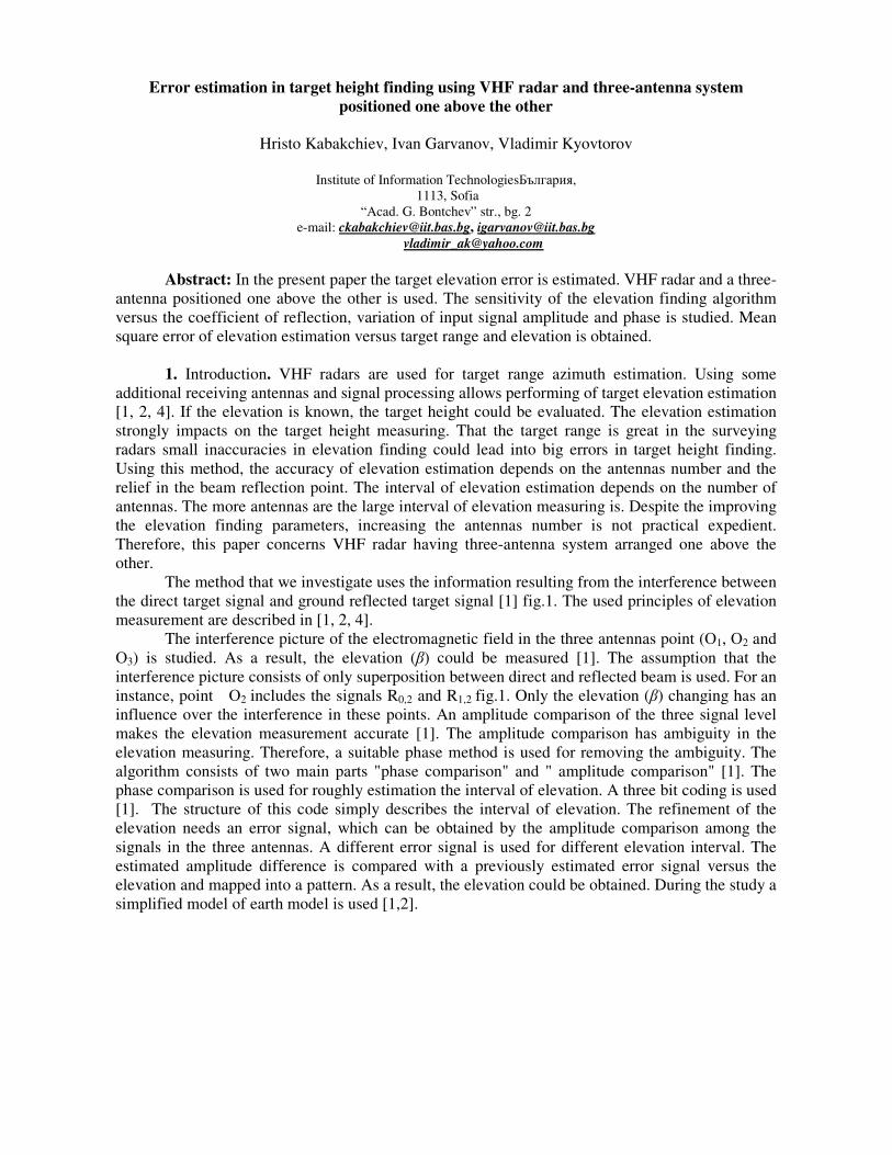
coefficient estimation for the pattern. The closer to the radar the point RB,I is, the more accurately the reflection coefficient could be estimated. As a result, the elevation could be measured more precisely. It can be seen the higher the active antenna is, the larger distance of the reflection point is. The consideration for choosing the active antenna results from the fig. 8. It is obvious that the active antenna having 7m height is more suitable than the 12m.

Fig.9 The signals in the three antennas and the coded phase differences between them versus the elevation in the mean square error of the relief height �h = 1m.

Fig.9 shows the character of changing the curves serving for roughly and fine estimation the elevation interval (fig.2) when the mean square error of the relief height is �σ =1m (o.s. fig.10). Here can be concluded that if an error is considered the graphics of the different signals change, which leads to error of elevation estimation after the comparison with the pattern.

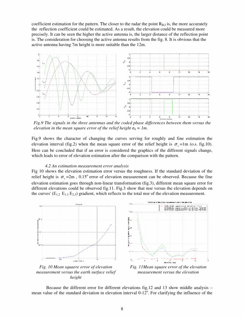
4.2 An estimation measurement error analysis Fig 10 shows the elevation estimation error versus the roughness. If the standard deviation of the relief height is �σ =2m , 0.15� error of elevation measurement can be observed. Because the fine elevation estimation goes through non-linear transformation (fig.3), different mean square error for different elevations could be observed fig.11. Fig.3 show that msr versus the elevation depends on the curves' (�1,2 �1,3 �2,3) gradient, which reflects to the total msr of the elevation measurement.

Fig. 10 Mean squaere error of elevation

measurement versus the earth surface relief height

Fig. 11Mean square error of the elevation measurement versus the elevation

Because the different error for different elevations fig.12 and 13 show middle analysis –

mean value of the standard deviation in elevation interval 0-12�. For clarifying the influence of the

9

gradient on the elevation error estimation two curves with different gradients are presented (�1,2 and �1,3). Fig.12 shows the mean standard deviation versus the inconsistence of the three channels. It can be observed, if the channels have 10% inconsistence, the error of elevation estimation reaches 0.5�. Fig.13 shows the mean standard deviation versus the amplitude signal noise ratio in the input of the channels amplifiers.

Fig. 12 Summed mean square error of elevation

measurement versus the inconsistence in the analogue channels

Fig. 13 Summed mean square error of elevation measurement versus the signal to noise ratio

Fig.3, fig.12 and fig.13 show that the lower curve gradient is prerequisite for a higher msr.

Fig.11, 12 and fig.13 are obtained in the MATLAB environment through Monte-Carlo simulation wit 50 statistical independent iterations.

4.3 The total error of height measurement analysis

Fig, 14 shows the mean square error of the target height versus the total elevation error (00 - 10) for different range measure accuracies. Results are obtained with the following input parameters: target range R01= 100 km, target range accuracy acc R01 = (0 m, 500 m, 1 km, 10 km), target height HT = 10 km. Fig. 14 shows that the range accuracy has not great influence on the target height estimation. From the other side, the elevation has considerable influence on the height accuracy estimation fig. 15. Increasing the elevation error, msr of error estimation has linear increment, as elevation msr 10 leads to height estimation error 1800m.

Fig. 14 msr of target height estimation versus

the total elevation error Fig. 15msr of target height estimation versus the total elevation error for different target

ranges

10

In this situation, the greater the target range is, the greater the height estimation error is. At

the fig.15 the target has height 10km and target ranges R01= 100, 200, 300 km are used. Fig. 16 shows the target range influence on the target height estimation accuracy. The greater target range is, the bigger msr of target height estimation is. The bigger the elevation estimation error is, the greater the target height estimation is. If the msr on the elevation estimation is in the interval +/- 0.10, the radar will have target height estimation error less than 500m. Fig.17 shows the msr of the target height estimation as a percentage of the target range. An error 0.2% of the target range is observed for msr of elevation estimation 0.10.

Fig. 16 msr of target height estimation versus target height for different elevation accuracies

Fig.17 Msr of target height estimation versus the target range for different elevation accuracies; related to the target range

Fig. 18 and 19 show percentage target height msr dependence on the target range and target

height. At fig.18 can be observed that the height changing from 5km to 30km doesn't influence on percentage msr of the target height measuring. The fig.19, which is made for R01=100 km, confirms this fact, as well.

Fig. 18 Msr target height estimation versus the

elevation error related to different target ranges; in percents

Fig. 19 Msr of target height estimation versus the elevation error related to different target

heigh;t in percents The results above, in the point 4.3, are obtained considered the total error of elevation measurement, or the sum error of:

- Roughness; - Inconsistence of amplitudes and phases in the three front-end channels; ; - SNR;

11

Fig. 20 shows the boundary line for msr of target height estimation 800m. Beneath the line is the target height, which could be measured with msr less than 800m versus the target range. For example, a target height 4km could be measured with accuracy 800m if the target range is up to 150km. If the target range is more than 150km, the msr of target height 4km is more than 800m. For comparison, the curves describing 0.5 and 0.9 of radio horizon are drawn. The curve is obtained in MATLAB environment through Monte-Ccarlo simulation with 200 statistical independent iterations. Three graphics are made for various height of the active antenna and various msr of target range measurement (std hRt = 23m and std hRt = 300m). It can be inferred that the active antenna height and the msr of target range measurement doesn’t have great influence on the target height estimation. More detailed, the active antenna height 7m gives better height estimation in scope up to target range 250km, next the active antenna height 12m gets the upper hand.

Fig. 20 a boundary line for msr of target height estimation 800m versus the target range.

12

Fig.21 shows the boundary curves for msr of target height estimation 800m using different

methods of target height estimation. The figure is similar to the fig.20 except the NEBO curve [5]. Considering the msr of elevation measurement 1,5�, according to the NEBO specifications, the NEBO curve shows the minimal target height, which could be measured at all, and the msr of the target height estimation in each point corresponding to a target range (50km 100km 150km 200km). Because the main characteristics of NEBO are given for elevation more than 50 [5], elevations less than 50 are not considered. For example considering elevation msr 1,5� , if the target range is 100km, the min target height that could be measured by NEBO is 9km with the accuracy of height measurement 2.6km. The other curves show the boundary lines only for target height msr 800m. Three positioned systems having different range measurement accuracy are shown (correspondingly "acc r1=r2=r3=300m" � "acc r1=r2=r3=23m"). Moreover, the accuracy of target height estimation versus various bases is shown (a=b=70� , 90� , 120� and 150 � .). For comparison, the line of active antenna height 7m and target range 300m (the curve at fig 20) is applied.

Fig. 21 a boundary line for msr of target height estimation 800m versus the target range. Mrs of using other methods of target height estimation (three-antenna

system positioned one above the other, three antenna multi-positioned antenna system, and NEBO)

13

5. Conclusion: Changing the height of the radar antennas could change the mutual phase angles of the interfering signals in them. As a result, the gradient of the error curves in various intervals could be changed (fig.3). This leads to increasing the accuracy of elevation measurement in some intervals, it is mentioned in [1] as well. The phase pattern, which is used in the current investigation, is made on the base of smooth surface (roughness D=0), lack of white gaussian noise, and lack of inconsistence between the channels. For development this pattern should be corrected in order to maximally compensate the factors giving the error. Fig.9 shows an example phase pattern for fine elevation estimation if the mean roughness in the reflection point is 1m in order to compensate the standard deviation of relief height 1m. There is a possibility of lack of the algorithm for rough estimation. The rough estimation of the interval of elevation couldn't be performed due to big errors of the interfering signals ((5), (6) and tab.1). Tab.1 [1] shows only 4 combinations, but 8 are possible. During the simulation of MATLAB we had a combination inexisting in the mapped table, an example situation is given bellow:

12Φ 13Φ 23Φ 1 1 0

Therefore, some solutions should be applied in order to eliminate the risk of not working algorithm. 6. Literature 1. Chen, B., G. Liu, S. Zhang “Method of Altitude measurement based on Beam Split in

Multi-antenna VHF Radar”, Proc. of International Conference on Radar System – RADAR 2004, CD –

2. ������� �., “���������� �� ������������”; �� 1; ������ “��������� �����” 1976�.

3. Skolnik, M., “Introduction to radar systems”, NK: Mc Graw-Hill Companies, 2001. 4. Barton, D., Leonov S.; “Radar encyclopedia ”;Artech house, inc., 1998; Norwood; 5. ���-���; ������������� �� ���-������������!���� ������ � �������"����";

"������� � � ��� � ������ ���� ���� � ���� �� ������ ���� � ����� "����-��""

7. Abbreviations: msr – mean square error