vertical relationships and competition in retail gasoline
TRANSCRIPT
PWP-075
Vertical Relationships and Competition in RetailGasoline Markets:
Empirical Evidence from Contract Changes inSouthern California
Justine Hastings
November, 2000(Revised: April 2002)
This paper is part of the working papers series of the Program on Workable EnergyRegulation (POWER). POWER is a program of the University of California EnergyInstitute, a multicampus research unit of the University of California, located on theBerkeley campus.
University of California Energy Institute2539 Channing Way
Berkeley, California 94720-5180www.ucei.berkeley.edu/ucei

Vertical Relationships and Competition in Retail
Gasoline Markets
Empirical Evidence from Contract Changes in Southern California
Justine S. Hastings Dartmouth College
Email: [email protected]
Abstract
This study examines how much, if any, of the differences in retail gasoline prices between markets is attributable to differences in the composition of vertical contract types at gasoline stations in each market. The purchase of the independent retail gasoline chain, Thrifty, by ARCO provides a unique opportunity to examine the effects of changes in different vertical contract types on local retail prices. This event caused sharp changes in the market share of i) fully vertically integrated stations, and ii) independent stations; differentially affecting local markets in the Los Angeles and San Diego Metropolitan areas. Using unique and detailed station-level data, this study examines how these sharp changes affected local retail prices. The detailed data and the research design based on the Thrifty station conversions allow for credible estimation of the effects of the market share of independent retailers and vertically integrated retailers on local market prices, controlling for any omitted factors at the station level, and the city level over time. Results indicate that a decrease in the market share of independent stations has a significant positive impact on local retail price. However, a change in the market share of refiner owned and operated branded stations does not have a significant impact on local market price. These results have important implications as policy makers consider the regulation of vertical contracts as a means to increase competition in gasoline markets. The research design and detailed data also allow for inference on the underlying nature of retail gasoline competition.
______________________________ I would like to thank Severin Borenstein, Kenneth Chay, and Richard Gilbert as well as Patricia Anderson, John DiNardo, Aviv Nevo, James Powell, Paul Ruud, Jonathan Skinner, Douglas Staiger, Miguel Villas-Boas and an anonymous referee for their valuable comments. I would also like to thank participants in the Labor Lunch and Industrial Organization Seminars at UC Berkeley. In industry I would like to thank MacDonald Beavers for valuable input, and for providing a unique data set. My research received funding from the UC Energy Institute and the Ohlin Foundation for Law and Economics.

2
I. Introduction
Since the late 1990’s, West Coast cities have consistently experienced substantially higher retail
gasoline prices than other regions of the country. For example, for the first week of August 1999,
the price of reformulated gasoline in California was 39.6 cents higher than the average price in
Gulf Coast States (about ten cents of this difference can be attributed to higher taxes in
California)1. In addition gasoline prices vary greatly between West Coast cities. Residents in San
Diego have paid a consistent five to fifteen cents more per gallon, on average, than Los Angeles
residents. These recent price phenomena have sparked intense political debate over the causes of
persistent price disparities. Much of the debate is centered around the effect of vertical contracts
between refiners and retail stations on retail competition and price levels.2
Industry trade organizations, politicians, and consumer groups have noted corresponding
increases in the number of fully vertically integrated gasoline stations in cities experiencing
higher citywide average prices. Because of this correlation, some form of divorcement legislation
has been considered in most West Coast cities and states. Divorcement legislation prohibits or
restricts the number of stations that a refiner can own and operate directly. Proponents of
divorcement argue that a larger market share of vertically integrated stations lessens competition
between refiners and increases their market power since the refiner directly sets the retail price at
this type of station. The fully vertically integrated station is usually referred to as a company-
operated (company-op) station. Divorcement would require the refiner to convert these stations to
lessee-dealer stations or open-dealer stations, where a dealer sets the retail price but is required to
pay the refiner's wholesale price, under the assumption that this would result in a lower, more
“competitive” retail price.
Another argument that has received much less attention claims that recent decreases in the
number of independent, unbranded retailers have decreased retail competition, since these
stations typically compete on price with little non-price product differentiation. Independent
stations are completely independent from the refiner in that the gasoline dealer owns the station,
and sells "unbranded" gasoline. The fact that the gasoline is unbranded allows the dealer to
purchase the lowest price wholesale gasoline available. They are not under contract to sell any
1 Source: Energy Information Administration, and California Energy Commission. 2 Midwest and East Coast have also experienced high gasoline prices and significant retail price differences between neighboring cities. As a result, the regulation of refiner's contracts with their retail stations has become a national issue. State government officials are currently lobbying congress for regulation of these contracts.

3
particular brand of gasoline or purchase from any given refiner, but cannot post a refiner's brand
name on their station. The unbranded station therefore competes with other stations by offering
the lowest price gasoline. When these stations are replaced by branded stations (or exit the
market), price competition in the market may be softened, resulting in a higher equilibrium price.
This analysis uses an event that caused sharp changes in the market shares of independents and
company-ops to determine their effects on local retail prices. The “long-term lease” of
approximately 260 independent Thrifty gasoline stations by Atlantic Richfield Company (ARCO)
provides an opportunity to test both the effects of company-operated and independent retailers on
local prices. The independent Thrifty stations were converted to ARCO stations with various
vertical contracts. These station conversions provide a “quasi-experiment” for testing the effects
of a change in a station's contract type on a nearby competitor's price. The Thrifty stations were
distributed across Southern California. Thus, the station conversions differentially affected local
markets within the Los Angeles and San Diego metropolitan areas.
These discrete and differential changes in the market share of company-ops and independents
allow for a pre-post comparison between affected and unaffected markets. This analysis compares
the price changes at stations located in markets affected by the conversion of an independent
Thrifty to an ARCO station, with price changes at stations in unaffected markets in order to
determine the effects of independent competitors on retail prices. Of the stations in affected
markets, the analysis compares price changes in markets with a new company-op ARCO versus
price changes in those with a new dealer-run ARCO, to test the divorcement hypothesis that an
increase in the market share of company-ops leads to higher prices.
To implement this approach, the analysis uses a new, unique and highly detailed data set of
station-level prices and characteristics for retail gasoline stations in the greater Los Angeles and
San Diego metropolitan areas. The discrete nature of the Thrifty station conversions, coupled
with the detailed station-specific data allow for the inclusion of station-specific fixed effects that
control for important determinants of retail prices that confound cross-sectional analyses. In
addition, the fact that many local markets within each metropolitan area were unaffected by the
conversions allows for the inclusion of city-time effects in the regression analysis - controlling for
any potentially unobserved factors that affected retail prices in any of the metropolitan areas in
any time period. The results indicate that stations competing with a Thrifty station had a
significant increase in price, relative to unaffected stations, after the independent Thrifty was

4
converted to an ARCO station. This increase was independent of the type of contract at the new
ARCO station, indicating that the type of contract at the branded station did not affect market
price, but the loss of an independent unbranded competitor did.
In addition to providing a credible approach to identifying the effects of independents and
company-ops on retail prices, the research design employed in this study provides a unique
opportunity to examine different models of retail competition in the gasoline industry. The
empirical results support a model of price competition with differentiated products and consumer
brand-loyalty.
The paper proceeds in seven sections. The first section gives a brief industry background. The
second section describes the existing empirical literature on the relationships between vertical
contracts and retail gasoline prices. The third section describes the long-term lease of the Thrifty
stations and the research design. The fourth describes the data, and the fifth section presents the
results and interpretation. The sixth section examines different models of retail competition, and
is followed by a conclusion.
II. Industry Background and the Potential Price Effects of Independents
Gasoline is produced by a refiner and then transported to a main distribution center called a
Distribution Rack. There are two types of gasoline: branded and unbranded. Branded gasoline has
an additive that is mixed into the gasoline just before it is taken for delivery to a retail station. For
example, in order to be called “Chevron” gasoline at the retail station, the gasoline must contain
the additive Techron. A similar requirement holds for Shell, Texaco, Exxon, and most of the
other brands available on the market. Under these requirements, a branded retail station must sell
the branded gasoline its sign displays.
A. Branded Gasoline Contract Types
If a retail station is a branded station, it can have one of three basic vertical contract types with
the branded refiner. The first type is a company operated station (company-op). Divorcement
legislation targets this type of station. The refiner owns the station and an employee of the refiner
manages the station. The refiner sets the retail price directly and pays the employee a salary. The
second type of station is called a lessee dealer. In this case the refiner owns the station and leases
it to a residual claimant. The lessee is responsible for setting the retail price, however he or she is

5
under contract to purchase wholesale gasoline directly from the refiner at the wholesale price the
refiner sets for a station in that “zone”. 3 This wholesale price is called the Dealer Tank-wagon
price (DTW).4 In addition, the refiner also sets volume discounts, the lease rate, and other
operation stipulations for the station. At the third type of branded station, a dealer owned station,
the retailer owns the station property and signs a contract with a branded refiner to sell its brand
of gasoline. The station displays the sign of the brand it is under contract to carry. The retailer can
either be supplied directly by the refiner (dealer-owned company-supplied) in which case they
pay a DTW, like the lessee dealer does, or the dealer can be supplied by a "jobber". A jobber is an
intermediate supplier who purchases gasoline at the distribution rack and pays a wholesale price
called the rack price. The rack price is the refiner’s posted price for branded gasoline at the
distribution rack, and it is the same price for any jobber purchasing at that rack. One jobber often
supplies, and possibly owns, many different branded and unbranded stations.
B. Independent Retail Stations
The above three types of stations sell branded gasoline. For example, a typical Shell station could
be any of those three types. If a station sells unbranded gasoline, it is an independent gasoline
station. Examples of independent retail chains include Rotten Robbie, E-Z Serve, Gas City, and
USA. These stations can sell any type of gasoline and can purchase it from any refiner selling
unbranded (or branded) gasoline at the rack price.5 Unlike the branded stations at which the retail
price of gasoline is directly set (at company-op stations) or indirectly influenced by the branded
refiner through lease terms, wholesale prices and volume discount rates, the independent retailer
can shop for the lowest wholesale price from any distribution rack and separately determine the
retail margin.
Independent retailers compete on price, offering no brand differentiation, and few of the
amenities (such as car washes or fast-food chains) that are offered by integrated branded retailers.
What does economic theory predict would be the effect on local market price when an
independent station changes to a major branded station of any vertical contract type? The
predicted price effect depends on the assumptions placed on the nature of consumer choice and
competition. For example, in a model where consumers have independent and identically
distributed tastes for gasoline brands/quality, price competition with other branded stations will
3 Zone pricing is used extensively in large metropolitan areas. A “zone” can be as small as one particular station. 4 DTW includes delivery to the station. 5 Jobbers can purchase branded gasoline and supply it to independent stations if it is cheaper than the unbranded price (the rack prices are “inverted”), but the independent station cannot post the name of the brand that they are selling. Hence, consumers do not know that they are purchasing branded gasoline.

6
intensify when an independent station becomes branded, thus lowering the market price for all
firms towards marginal costs. However, if becoming a branded station allows stations to increase
price because a proportion of consumers value that brand over all others (brand loyalty), the new
branded station may increase its price, and competitors will increase their prices in response.
Thus, in a model of price competition with differentiated products, the predicted price effect of an
independent retailer becoming a branded station, all else equal, depends on the assumptions
placed on consumer preferences, and thus how the change will affect the station's demand, own
and cross price elasticities.
The purchase and branding of the independent Thrifty stations by ARCO provides an opportunity
to estimate the effects of independent retailers on local competitor's prices without requiring, a
priori, the structural specification of retail demand and competition. In the end, the research
design will also be used to make inferences on the underlying structure of retail competition.
III. Empirical Literature
The effect of independent marketers on retail price levels has not been considered in the
literature. The main focus has been on the choice of contract type between the refiner and the
branded station: the choice between company operation or lessee dealership for the stations that a
refiner owns. If the retail price is set by a residual claimant with market power, as the case may
be for dealer-run stations, the dealer may set a super-competitive mark-up over the refiner's
wholesale price of gasoline. A company-operated station does not have this second margin,
therefore the company-op contract may lead to lower prices since it avoids the double
marginalization problem. Borenstein, Cameron, and Gilbert (1997), Borenstein and Shepard
(1996), and Slade (1992) provide empirical evidence consistent with local retail market power.
Because of this potential for retail market power, many studies of contracts between gasoline
stations and refiners have focused on the trade-off between double marginalization and
monitoring cost, and hence the refiner's choice between company operation and lessee dealership
at the stations it owns. Shepard (1993) applies a principal-agent analysis to examine the refiner’s
choice of vertical contractual form observed at a cross-section of retail gasoline stations in
Massachusetts. She finds evidence that stations with amenities such as service bays, that would
require higher monitoring costs by the principal, tend to be dealer-run, and those with small

7
monitoring costs, stations that mainly sell gasoline and convenience store products, tend to be
company operated.
Rey and Stiglitz (1995) show that in differentiated product markets, wholesalers may also have
strategic motives for vertical separation, especially when they can use quantity incentives and
franchise fees (both available in the lessee-dealer contract) to extract retail profits. The vertical
separation can decrease the wholesaler's perceived demand elasticity, resulting in higher retail
prices, and producer's profits when a two-part tariff can be used to extract retail profits. In their
model, it is the lessee-dealer contract, and not company-operation, that is chosen by the
wholesaler to decrease retail price competition. Using retail contract data for gasoline stations in
Vancouver, Slade (1998) finds some evidence supporting strategic motives for vertical
separation. Both the double marginalization and the strategic-motives models imply that, ceteris
paribus, dealer-run stations will have higher prices than company-ops when retailers have market
power.
Barron and Umbeck (1984) used data on retail gasoline prices from a refiner survey in Maryland
to test the double marginalization hypothesis by analyzing the effects of Maryland’s 1979
divorcement legislation. They used station level price data for 99 stations from a refiner survey
with at least one observation before and after the implementation of divorcement legislation.
They found that the price of regular self-serve gasoline at stations that were converted from
company operated stations to lessee dealers increased by 1.4 cents after the divorcement took
place. Their study provides evidence for the double marginalization hypothesis, and hence against
divorcement legislation. However, the study does not control for station-specific fixed effects or
time effects – important determinants of retail gasoline prices that may confound results if not
included.
There is a second body of literature that attempts to analyze the effects of divorcement legislation
for policy proposals or regulation. Most use city average prices to determine if divorcement
legislation would increase or decrease prices. For example, Vita (1999) uses monthly statewide
average gasoline prices to examine if states with divorcement legislation have higher or lower
prices than states without it. 6 The time period considered does not allow for a before and after
6 Hawaii, Connecticut, Delaware, Maryland, Nevada, Virginia, and District of Columbia have all had divorcement for the sample period considered. The legislation in Nevada was passed in 1984 in response to high sustained retail prices following an expansion in the market of company-op gasoline stations. The legislation ranges from prohibiting

8
comparison, since the states with divorcement had the legislation in place throughout the sample.
Based on the state-average retail prices, he finds that divorcement legislation is associated with a
2.7 cent higher prices. This is interpreted as evidence that divorcement legislation causes higher
retail gasoline prices. This correlation may not be causal, since historically, high gasoline prices
have caused the proposal and passage of divorcement legislation. We would expect to see
divorcement legislation in states with higher average prices.
In fact, it is precisely higher average prices coinciding with increases in the market share of
company-ops that has spurred the recent round of divorcement proposals in West Coast cities.
Pro-divorcement groups note that the cities that have experienced the most dramatic increases in
average prices have also experienced increases in the market share of company-ops. These
examples center on Los Angeles, San Diego, Phoenix and Tucson. While it is true that the
number of company-op stations in these cities has increased, the correlation between this and the
increase in average prices may not be causal. Nearly all of the increase in company-op stations in
the West Coast over the past five years came from the purchase of two independent chains by
integrated refiners: 1) Thrifty by ARCO, which affected Southern California, and 2) Circle K by
Tosco, which mainly affected Phoenix and Tucson. 7 Therefore, at the citywide level of
aggregation, the increase in company-ops and the decrease in independents are perfectly
correlated. It is therefore unclear which, if either, of these two factors has had a positive impact
on retail prices.
The Thrifty case study coupled with detailed station-level data, allow us to separate the two
effects: the impact of company-ops and the impact of independents on retail prices. The micro-
data also illustrate that city-averages mask a considerable amount of retail price variation. By
using station-level data, this variation can be exploited to control for other potentially
confounding factors that affect retail prices within each metropolitan area.
IV. A Research Design Based on the Thrifty Purchase
A. Details of the Thrifty Purchase company-ops to capping their market share, to simply requiring a minimum distance between a company-op and a dealer-run station.

9
In March of 1997, ARCO announced the "long-term" lease of the majority of the independent
Thrifty gasoline stations in Southern California.8 The announcement was followed by a sixty-day
waiting period, after which ARCO assumed control of and branded the Thrifty stations.9 Thrifty
Oil Company was the largest independent chain of retail gasoline stations in Southern California
with approximately 260 stations ranging from San Diego to Santa Barbara. The next largest
independent retail chain – USA - has only 32 stations in Los Angeles. Thrifty stations were
located all over the Los Angeles and San Diego basins. Almost all stations were included in the
long-term lease by ARCO and this event accounts for practically all of the changes in the
percentage of company-op stations in Los Angeles and San Diego as well as the decrease in
independent retailers during the 1990’s.
After the sixty-day waiting period, ARCO branded the Thrifty stations and completed the
branding by September 1997. ARCO branded the stations, meaning that they simply changed the
colors and added ARCO gasoline signs to the Thrifties, but no remodeling or station expansion
was done during the period considered in this study. Some of the Thrifty stations were converted
to lessee-dealer ARCO stations, some were converted to dealer-owned company-supplied or
jobber-supplied stations, and some were converted to company-ops. Approximately two thirds of
the stations became company-operated ARCO stations, and the remainder were dealer-run.
B. Research Design
Ideally, to test the effects of independent market share and company-op market share on retail
prices, the researcher would randomly re-assign vertical contracts at a sample of stations. The
resulting change in local prices would then be observed, and causal relationships identified.
Random assignment ensures that the differential changes in the market share of company-ops and
independents are orthogonal to all other factors that determine retail prices.
7 Because the Circle K purchase differed in key ways from the Thrifty purchase, it is being examined in a separate study. Tosco owns the Unocal refining and marketing assets on the West Coast, including refineries, retail stations, and the Union 76 brand. 8 The specific details of the long-term lease were not disclosed. ARCO officials state that the stations were not purchased because the lease agreement was a more affordable option. The stations were re-branded and are operated like any other ARCO station. A few stations were not included in the lease because they were substandard and needed renovation and underground storage tank replacement. All information about the lease was obtained by conversations with ARCO and Thrifty Oil Company officials, and from press releases from ARCO. 9 Thrifty Oil Company was a privately held company. The owner was 75, and decided to retire and sell the company's retail assets to ARCO. ARCO saw this as a good opportunity to expand market share. This is the official reason for the agreement given in all press releases and by officials from either company.

10
Since the random assignment of station contract and ownership types is not possible, one solution
is to use sharp discrete changes in contract types provided by the Thrifty purchase to dramatically
reduce the omitted variables bias problem in estimating the effects of company-op and
independent market share on retail prices. The data are a panel of station-specific prices available
for the months of February, June, October, and December of 1997 in the greater Los Angeles and
San Diego metropolitan areas. Thus there are observations before and after the station conversion
period.
Because of the wide geographic dispersion of the Thrifty stations, local markets in Los Angeles
and San Diego were differentially affected by the station conversions. The gasoline stations are
grouped into local sub-markets of stations in direct competition with each other.10 Some stations
competed with a Thrifty, and some were not located near any Thrifty station. Therefore, the
“treatment” effect of a discrete change in a competitor’s contract type differentially affects the
stations in the sample. These discrete and differential changes allow for pre-post comparisons
across affected and unaffected markets to estimate the effect of independents and company-ops
on prices, conditioned on station-level fixed effects and city-time effects. This research design
dramatically reduces the dimension of potentially omitted factors that may be correlated with
both prices and the parameters of interest.
The Thrifty purchase provides a credible approximation to random assignment of a change in the
market share of independents since the chain included approximately 260 stations that were
geographically scattered over the greater Los Angeles and San Diego basins. Their locations and
characteristics where predetermined to ARCO's acquisition decision. For this reason, it is
reasonable to treat the loss of an independent Thrifty as exogenous to a local competitor station's
pricing decision, conditioned on station-specific fixed effects and city-time effects.11 The “quasi-
experimental” research design examines how an individual station’s price is affected by a change
in a competitor’s contract type. A change in a competitor’s contract type, in this case, is not in a
station’s choice set, and is therefore treated as exogenous to the individual station’s pricing
decision, conditioned on fixed effects and time effects.12 In addition, the Thrifty stations were
simply rebranded by ARCO and placed under new contracts, without remodeling, expansion, or 10 The analysis uses geographic proximity to determine local markets. The markets definition is described in section V.B., and in greater detail in Appendix A. Results are tested to ensure that they are not driven by market definitions. 11 The data only include price observations on 5 of the Thrifty stations, so we use price data on local competitors to estimate the effect of the Thrifty station conversions on local market prices.

11
12 The percent of each brand present in the treatment group (stations that competed with a Thrify) approximately reflects the percent of each brand in the station population, adding evidence that the Thrifty chain was fairly evenly distributed among different brand competitors.
Figure I: Map of Thrifty Stations in Los Angeles Metropolitan Area. Squares with flags denote a Thrifty Station

12
other facility improvements. These facts allow for credible estimation of the effect on a station’s
own price of a change in the market share of independent competitors.
While the location and characteristics of the Thrifty stations were predetermined to the ARCO
purchase, ARCO chose which stations to convert to company-ops and which to convert to
dealers. The discrete timing and differential assignment of these changes significantly reduces the
potential omitted variables problem present in cross-sectional or time series analysis of the effects
of company-op market share on retail prices. However, because the contract decisions where
made by a profit maximizing firm, there is a potential for confounding omitted factors that are
correlated with both prices and the location and timing of the company-op contract assignment.
For example, suppose that ARCO chose company-op contracts for stations in markets with
relatively low price elasticity, and ARCO pursued a pricing policy of greater price discrimination
at these particular stations after their conversion. Then this pricing policy change is correlated
with the location and timing of the company-op contract assignment, and may inhibit the
identification of the general effect of company-ops on retail prices. This potential endogeneity
problem is discussed further in Section VI.
If it is the case that the increase in company-op stations lowers competition and increases market
price, then the stations that compete with a Thrifty that was converted to a company-op ARCO
should have a larger price increase than those stations that compete with a Thrifty that was
converted to a dealer operated ARCO, all else equal. The data analysis presented in this study
will show that this is not the case. The analysis lends strong empirical evidence supporting the
hypotheses that independent retailers have a significant negative impact on competitor’s prices,
and that when they exit the market, local retail prices increase. This price increase is independent
of the resulting contract at the branded station – indicating that an increase in the market share of
company-op stations is not correlated with an increase in market price as the divorcement
hypothesis would contend.
V. The data
A. Description and Summary Statistics
The first data set used in the analysis is an annual census of retail gasoline outlets in the Los
Angeles and San Diego metropolitan areas. The census gives detailed information on the outlet
characteristics including: type of convenience store, size of convenience store, number of pumps,

13
service bay, size of service bay, fast food chain, car wash, and location, among others. It also has
the ownership and delivery type for each station, which determines if the station contract is
company-op, lessee-dealer, dealer-owned-company-supplied, dealer-owned-jobber-supplied, or
independent. The second data set contains volumes and prices by grade and service for a sample
of the stations in the census report. The volumes were read from each gasoline station's pump
meters. The prices are the prices posted at the end of the volume collection period for the months
of February, June, October, and December in 1997. The sample size varies by city from 20-25%.
The stations in the sample were chosen to reflect the market share of station types in the market.
If Chevron stations comprise 15% of the total census of stations, then 15% of the sample are also
Chevron stations that were chosen at random out of the population of Chevron stations.13
This data set makes it possible to separate the effects of changes in the number of company-op
stations and the number of independents on local retail prices. Station-level detail allows for a
comparison between local markets that were affected by the Thrifty purchase and those that were
not affected. For those that were affected, we can also compare the price changes in the markets
where the new ARCO station became a company-op with those in which it became a dealer-run
station. These comparisons would not be possible with aggregated data. In addition, the station-level data highlight the fact that there is as much price variation at the
station level as there is in the average prices across metropolitan areas. If the goal is to determine
the causes of average price differences between cities, it is important to first determine what
causes persistent price differences between stations within each city. Figure 1 presents kernel
density estimates for the February 1997 observation in Los Angeles and San Diego. The average
retail price in Los Angeles for self-serve regular unleaded gasoline was $1.273 in Los Angeles
and $1.320. This difference in average prices from this data is consistent with the citywide
averages used in industry studies. Figure 1 illustrates that the spreads of the price distributions
within each metropolitan area are larger than the difference in the average prices across
metropolitan areas. The variation within metropolitan area is as significant as the variation across
metropolitan areas.
Figure 1 also indicates that the lower tail of prices in Los Angeles drives the difference in average
price between Los Angeles and San Diego. This lower tail may be caused by many factors.
13 Data were collected by Whitney Leigh Corporation. The volume and price data were read directly from posted prices and pump meters at the stations, and are therefore more reliable than volumes and prices obtained through other methods such as telephone or manager surveys.

14
* Epanechnikov kernel function was used. Bandwidth was set at the minimum of the optimal bandwidths for Los Angeles and San Diego, where the optimal bandwidth is 5/1/9.0 nmh = , m=(σx, interquartile rangex/1.349)
For example, there are more independent retailers in Los Angeles than in San Diego. However,
Los Angeles also has a greater percentage of low-income neighborhoods, longer average
commute times, and a higher average retail station density. These factors could all lead to a larger
tail of lower priced retail outlets. This emphasizes the benefits of using the conversions of Thrifty
stations to ARCO stations to determine the effect of independents on local retail price. Due to the
geographic dispersion and the discrete timing of the changes, it is possible estimate the effects of
independent competitors on prices while controlling for station-specific fixed effects, such as
local commute patterns and retail station density. The fixed-effects absorb any unobserved
station-level factors correlated with both independent competitors and the local retail price level. With station level data we can use a variance components decomposition to examine the amount
of total price variation that occurs within a city over time. This variation would be lost when
using aggregated data. The variance components model assigns a random effect to each of the
categories in the table below. Since the Los Angeles and San Diego metropolitan areas cover such
a large geography, the data were further grouped by sub-city within the two metropolitan areas.
The sub-city classification groups the sample stations in their local cities, such as Chula Vista (in
-1
0
1
2
3
4
5
6
7
8
9
10
11
12
13
14
1.1 1.15 1.2 1.25 1.3 1.35 1.4 1.45 1.5 1.55
Los Angeles DensitySan Diego Density
Figure 1: Kernel Density Estimates for Retail Price of Regular Unleaded Gasoline in February 1997 Observations for Los Angeles and San Diego

15
the San Diego metropolitan area) or Pomona (in the Los Angeles metropolitan area). There are 56
sub-city regions in this analysis.
The variance components estimates show that there is as much variation at the station level over
time as there is at the city and time levels. Sub-city does not contribute much to the variation in
prices. City is important because of cost differences between Los Angeles and San Diego. All of
the refiners are located in Los Angeles, and there is one pipeline used to transport product for
distribution in San Diego. Each refiner can make approximately one shipment per week. Because
of this, transportation cost to stations in San Diego area are higher than to those in Los Angeles,
and prices in San Diego will experience differential trends in prices when there are supply shocks
to refineries in Los Angeles. Hence City and City-time are important determinants of retail prices.
Within each city, local markets are smaller than the Sub-city level, hence Sub-city classifications
account for little of the total price variation. This highlights the benefits of using station level data
instead of aggregated data in analyzing the effects of changes in retail market composition on
prices. The importance of station level data will become evident again in the final fixed-effects
estimation and in the examination of the underlying models of retail competition presented in
Section VIII.
Table III: Variance Components Estimation
Component Variance Component Estimate Percent of Total Variance
Month 0.00308 0.26506
City 0.00334 0.287435
Sub-City 0.00032 0.027539
City*Month 0.00104 0.089501
Sub-City*Month 0.00036 0.030981
Station-time (residual) 0.00348 0.299484
B. Retail Market Definition
The retail market definition used in the regression analysis presented below is the following: A
station with a price observation competes with any station within 1 mile along a surface street or
freeway. Therefore, a station with a price observation competes with a Thrifty if there is a
Thrifty located within one mile. The detailed address information provided by the census data
allows for a realistic geographic definition of sub-markets. Although it is true that people in
Southern California commute a lot, making it harder to tell which stations compete with each

16
other (stations near your house may compete with stations near your work), this definition
attempts to capture the stations that compete most intensely for customers in their area. In order
to confirm that the results were not driven by geographic definitions, the regressions were run
using perturbations of these definitions, and the results were robust to these changes. The
perturbations increased or decreased the scope of the definitions by half a mile. The signs and
significance of explanatory variables remained the same, although the magnitudes varied slightly
by a statistically insignificant amount.
The above market definition includes factors considered by dealers and refiners to be main
determinants of competition. According to dealers, refiners, and trade groups, stations in Los
Angeles and San Diego compete most intensely with any station within 1 mile.14 This definition
is further reinforced by the fact that stations of the same brand are usually located more than a
mile apart. In addition, many contracts between dealers and refiners stipulate that the refiner will
not brand another station within one mile of that dealer’s location. By graphing the stations using
mapping software, it is possible to examine each station’s nearest competitors. A more detailed
description of competition groups and geographic definition is presented in Appendix A. The
regressions presented in Appendix A also highlight the problems introduced by geographic
aggregation in estimating the parameters of interest.
VI. Results
A. Graphical Analysis
Even though it is possible to control for every recorded station characteristic, it is impossible to
control for many factors that are unobservable to the economist but may affect the local demand
and competition that a station faces. The “quasi-experiment” based on the Thrifty station
conversions provides a credible research design for identifying the effects of i) the market share
of independents, and ii) the market share of company operated stations on local retail prices.
Graphs I.a and I.b provide a rough estimate of the impact of independent retailers on competitors’
prices.
14 This information came from various conversations with regional managers, dealer trade organization representatives, and from conversations with various dealers at retail stations.

17
These two plots present the average price level in each time period for stations that were affected
by a Thrifty conversion, and thus lost an independent competitor, versus the average price level at
stations that were unaffected by the conversions. These figures illustrate that before the long-term
lease took effect, the stations that were competing with a Thrifty station (the treatment group) had
lower prices than the market averages for stations that never competed with a Thrifty in any time
Los Angeles Extended Treatment/Controll Graph
1.150
1.200
1.250
1.300
1.350
1.400
1.450
1.500
1.550
December February June October December
Ret
ail P
rice
Reg
ular
Unl
eade
d
Competed with a Trifty
All Other Stations
San Diego Extended Treatment/Controll Graph
1.15
1.2
1.25
1.3
1.35
1.4
1.45
1.5
1.55
December February June October December
Ret
ail P
rice
Reg
ular
Unl
eade
d
Competed with a Thrifty
All Other Stations
Graph I.b: San Diego Treatment and Control Graph
Graph I.a: Los Angeles Treatment and Control Graph

18
period (the control group). This relationship is the same in both Los Angeles and San Diego, even
though the two metropolitan areas experienced differential trends in prices over this period.
Within each graph, the pre-conversion trends of the two averages are identical. The pre-
conversion and post conversion price difference between the two groups is also similar across
metropolitan areas.
After the conversion period, the stations in the treatment group had a higher price than the
average price of stations in the control group.15 Based on this graphical analysis, the stations that
competed with an independent Thrifty had roughly a two to three cent lower average price than
other stations before the conversion. After the conversions, these stations had about a two to three
cent higher average price than other stations, indicating a price increase of four to six cents
resulting from the conversion of an independent Thrifty station to an integrated ARCO,
independent of the subsequent contract type. These graphs provide preliminary evidence that
presence of an independent competitor is associated with a four to six cent lower local market
price.
If the stations in the treatment group (stations that competed with a Thrifty) are divided into two
groups: i) stations that now compete with a company-op station, and ii) those that now compete
with dealer, a similar graphical analysis can be performed. This provides a rough estimate of the
impact of an increase in company-ops on local market prices. Graphs II.a and II.b summarize the
price effect of a Thrifty becoming a company-op ARCO verses a dealer run ARCO that the fixed-
effects regression analysis estimates. The graphs show no apparent difference in the price
behavior between stations that compete with a new company-op ARCO and those that compete
with a new ARCO dealer.
Notice that, within each metropolitan area, the pre-buyout and post-buyout levels and trends are
very similar between the two groups. One group does not appear to display a persistently different
pattern than the other. This is consistent with “exogeneity” of the contract assignment to other
station-level factors that may be correlated with price. Since there is no clear trend in relative
prices between the two groups in either metropolitan area, these two graphs imply that an increase
in company-ops does not have a significant effect on local retail prices. The four graphs together
15 Almost all of the stations were rebranded after the June observation and by about the end of August. A few of the Thrifty stations in the sample were changed to ARCO stations before June. These stations are not included in this graph. In the regression, they have the appropriate timing. These graphs show the majority of the affected stations – those that were converted between the June and October price and volume observations.

19
lend preliminary support to the hypothesis that the presence of independent competitors, and not
the presence of company-ops, has an impact on local competitor’s prices.
San Diego
1.150
1.200
1.250
1.300
1.350
1.400
1.450
1.500
1.550
December February June October December
Ret
ail P
rice
Reg
ular
Unl
eade
d
Changed to Dealer
Changed to Company-op
Los Angeles
1.15
1.2
1.25
1.3
1.35
1.4
1.45
1.5
1.55
December February June October December
Ret
ail P
rice
Reg
ular
Unl
eade
d
Changed to Dealer
Changed to Company-op
Graph II.a: Los Angeles Change to Company-op vs. Change to Dealer-run
Graph II.b: San Diego Change to Company-op vs. Change to Dealer-run

20
B. Random Effects Estimation
A first attempt at estimating the effect of changes in a competitor’s contract type on another
station’s price is a pooled regression analysis, assuming a linear relationship between stations’
prices and a vector of covariates. This model can be written as:
ititititit zcwp εθφβα ++++= where pit is station i’s price for self-serve regular unleaded gasoline at time t, cit is the market
share of company-op competitors in station i’s market at time t, zit is the market share of
independent competitors, and wit is the vector of all other determinants of station i’s prices.
In principle, if all of the determinants of a station’s price decision were observable and
measurable, then the relationship between contract type on retail prices could be identified. In
reality, many of these determinants are not observable to the researcher, and their omission may
bias the estimation results. A standard least-squares analysis will lead to inconsistent estimates of
the impact of independents and company-ops on retail prices if the researcher cannot control for
all factors that affect prices and vary with independent and company-op market shares.
The pooled regression in Table IV is specified as:
itiitititit uzcxtp εθφβδγα +++++⋅+= where: α = constant
γ = city dummy t = time dummy xit = vector of observable station characteristics cit = indicator for if a competitor becomes a company operated station zit = indicator if the station competes with an independent Thrifty station16 ui ~ N(o, σu
2), εit ~ N(o, σε2)
16 This regression was also run with cit = number of company-ops station i competes with and zit = number of independents station i competes with. In this case, cit and zit are integers that stay constant over the entire period of observation, except for the stations that compete with a Thrifty. In this case zit changes from 1 to zero when the Thrifty becomes an ARCO, and cit increases by 1 if that new ARCO was a company-op. The estimates using these variable definitions show more bias in comparison to the fixed-effects estimates than those that use only the changes from the Thrifty station conversions. If the number of independents a station competes with is used, the coefficient on Independent in Column 4 is -0.0037 with a robust standard error of 0.0025. The coefficient is no longer significant. Note that the value for Independent stays constant over the sample period for all stations that do not compete with a Thrifty. Hence there is great potential for heterogeneity bias. It is only the discrete changes from the Thrifty station conversions that generate inter-temporal and cross-sectional variation in the number of independents a station competes with. This variation allows the price effects of independents to be identified separately from the price effects of other time-invariant factors. Please see footnote 20 for the fixed-effects results.

21
The results from the pooled regression with station-specific random effects are discussed below.
The random effects estimates are presented as a comparison for the final robust fixed effects
results. These results emphasize the importance of the research design using station level fixed
effects and city time effects.
Table IV presents the regression results for the Random-effects model. Company Operated is an
indicator for when a competitor becomes a company owned and operated station. This variable
changes when a competitor Thrifty station becomes a company-op ARCO station. Independent
indicates if the station competes with an independent station. This variable decreases discretely
when a Thrifty is changed to a branded ARCO station of any vertical contract type. The various
columns in the table show the changes in the parameters of interest as the regression models
consecutively control for station-level characteristics and city-time effects. The estimates in the
final column will be compared to the Fixed Effects estimates presented in Table V.
Column 1 of Table IV on the following page shows the unadjusted correlation between Company
Operated and retail prices. This is the estimate of the price effect of increases in company-ops
that is used to support divorcement legislation. The coefficient is large and significant. However
it is clear from the fourth column that the coefficients on Company Operated in the first three
columns are attributing the price effect of the contemporaneous citywide prices increase to
Company Operated. The same is true for the coefficient on Independent in column 2. Since the
timing of the company-op increases and independent decreases coincide with the market-wide
price increases shown in Graphs 1.a and 1.b, both variables are large and significant when city-
time effects are excluded from the regression. The coefficient on Company Operated is not longer
significant in column 4.
Columns 3 and 4 sequentially control for observable station-level characteristics and
demographics that may be correlated with retail prices, and for city-time effects. Of the station
characteristics, the presence of a Fast Food Chain (such as McDonald’s or Subway) is associated
with a three cent higher price than other stations, and is significant in column 3.17 However, the
coefficient becomes insignificant in column 4 when the city-time effects are included. In column
4, the coefficient on the Average Quantity of Food sold is significant at the two percent level. The
17 This may be due to the fact that the station can charge more since consumers only have to make one stop to purchase a meal and gasoline, so consumers are willing to pay more to avoid another stop.

22
Table IV: Pooled Regression: Estimated Effects of Company Operated and Independent stations on Retail Price of Regular Unleaded Gasoline (Robust standard errors in parentheses) Variable (1) (2) (3) (4)
Intercept 1.3302* (0.0022)
1.3302* (0.0022)
1.4025* (0.0353)
1.2916* (0.0279)
Company Operated 0.0581* (0.0084)
0.0516* (0.0083)
0.0515* (0.0097)
0.0123 (0.0076)
Independent - -0.0519* (0.0072)
-0.0549* (0.0055)
-0.0289* (0.0046)
Self-Serve Nozzles - - -0.0002 (0.0003)
-0.0001 (0.0002)
Ave. Quantity Food - - -0.0001 (0.0001)
-0.00015* (0.00006)
Snack Shop - - -0.0074 (0.0052)
0.0020 (0.0042)
Car Wash - - 0.0077 (0.0067)
0.0068 (0.0054)
Fast Food Chain - - 0.0299* (0.0140)
0.0141 (0.0120)
Service Bay - - -0.0025 (0.0051)
0.0028 (0.0040)
Credit Card - - 0.0077 (0.0058)
-0.0015 (0.0043)
Oil Change - - -0.0087 (0.0128)
0.0157 (0.0111)
Number of Stations within a mile
- - 0.0062 (0.0010)
-0.0022* (0.0008)
Distance to Nearest Competitor (in yards)
- - -0.0000001 (0.000002)
-0.0000004 (0.000003)
Per Capita Income In Census Tract
- - -0.0000009* (0.0000004)
-0.00000073* (0.00000034)
Percentage White Population In Census Tract
- - 0.1149* (0.0149)
0.0511* (0.0119)
Percentage of Workers using Public Transportation
- - -0.0355 (0.05136)
-0.0395 (0.0384)
Average Travel Time to Work
- - -0.0022* (0.0004)
-0.0002 (0.0004)
LA*June - - - 0.0065* (0.0029)
LA*October - - - 0.1223 (0.0039)*
LA*December - - - -0.0167 (0.0041)
SD*February - - - 0.0433* (0.0044)
SD*June - - - 0.0985* (0.0050)
SD*October - - - 0.1855* (0.0055)
SD*December - - - 0.1310* (0.0060)
Adj. R-Square 0.017 0.037 0.087 0.537 N = 2676
*Statistically significant at the 5% level or better

23
coefficient implies that as the average monthly dollar value of food products sold increases by
$100,000, the price at the station decreases by 1 cent. Since the sample average is approximately
$18.6 (measured in thousands), the magnitude of the coefficient implies that only stations with
the highest volume food sales have slightly lower prices.
The only other station characteristic that is significant is the Number of stations within a mile.
The coefficient implies that a station with 6 competitors within a mile would have one cent lower
price than a station with one competitor within a mile, all else equal. The sample mean for this
variable is 3.6, with a standard deviation of 2.1. Hence, price could vary by one cent a gallon for
stations within one standard deviation of the mean number of competitors within a mile, all else
equal. The researcher might think, a priori, that the other included station characteristics should
have a significant effect on a station’s retail price level. The fact that they do not suggests that
there are confounding, unobservable station-specific factors that are not controlled for. These
factors inhibit the pooled regression model from estimating the true contributions of each of these
variables to a retail station’s price.
Each station was mapped into a census tract, linking demographic data at the census tract level to
the individual stations. Demographic variables that may influence price elasticity are included in
columns 3 and 4. Of the demographic variables in column 4, both per capita income level and the
percentage of the population that is white are significant determinants of retail prices, once city-
time effects are controlled for. The coefficient in column 4 on Percent White Population indicates
that an increase of 0.10, or ten percent, in the percent of white residents in a census tract is
associated with a 0.5 cent increase in station price. This implies that a station in a census tract
with 70% whites would have a 1 cent higher price than the same station in a census tract with
50% whites. Per capita income levels are surprisingly negatively correlated with station prices.
Since income is in thousands, an increase in income of $100,000 would be associated with a
price decrease of 7.3 cents. Hence, an increase in income of about $13,700 would be correlated
with a decrease in station price of 1 cent. It is not clear why income should be negatively
correlated with price. The correlation coefficient between Income and Percent White is 0.588,
however neither variable changes sign or significance when the other is excluded from the
regression. It may be the case that there are other factors that are correlated with both income and
low prices that are not observable to the researcher. These factors may account for the negative
coefficient on income.

24
It is important to note that the station characteristics and demographic variables explain very little
of the total variation in prices. The fit of the regression in column 3 is quite poor, with an adjusted
R-squared of only 0.087. The inclusion of station fixed effects will significantly increase the
amount of station-level price variation explained, suggesting that there are many important
station-specific variables that are unobservable to the researcher, but are still significant
determinants of retail prices.
The City-time dummies are all significant. Recalling the differential time effects across cities in
Graphs I.a and I.b, it is not surprising that controlling for city-time effects considerably increases
the amount of price variation explained by the regression model. Notice that the coefficient on
Company-op becomes insignificant once these city-time effects are included. The discrete timing
and differential changes in Company-op and Independent across markets allows for city-time
effects that control for any citywide shocks to prices in any time period that confound the
regression results if not included. Controlling for city-time effects takes out the market-wide
trends in Graphs I.a and I.b, thus separating the effects of company-op and independent from the
coinciding market-wide price trends.
C. Fixed-effects Estimation
The parameter estimates in Table III are not consistent if the Random-effects specification is
incorrect. This specification assumes that the expected value of the station-specific error term,
conditioned on observable station characteristics, is the same across all stations. If the locations of
independent stations are correlated with an unobservable local market characteristic that also
influences price, this assumption is violated, and the Random-effects estimator is inconsistent.
For example, independent stations may choose to locate on local streets rather than directly off of
freeways because the station property is less expensive. This unobservable factor affects both
local market price and the presence of an independent. This correlation leads to heterogeneity
bias in the Random-effects estimate on Independent. The Fixed-effect estimator is the only
consistent estimator when the expected value of the station-specific error component, conditioned
on observables, differs across stations.
With the fixed-effects specification, the effects on price of any station or local market
characteristics that are time invariant cannot be determined independently from the fixed effect.
Hence city-wide effects cannot be estimated, nor can the effects on price of location, store size,
number of pumps, or service amenities, be determined separately from the fixed effect. However,

25
since there were large discrete changes in a key variable - a competitor’s ownership and contract
type - during the observation period, we can obtain consistent estimates of the price effects for the
variables most relevant to current policy decisions. It is precisely the discrete nature of the
conversions of the independent retail stations and their broad geographical distribution that allow
for convincing identification of the price effects of independents and company-ops. The station
fixed effects and city-time effects absorb any potentially confounding factors at the city, city-
time, time and station levels.
Station Level Fixed-Effects with City-time dummies:
itititiit zctp εθφδγαµ +++⋅++= where: µ = constant
αi = station-specific deviation from the mean µ γ = city dummy t = quarterly dummy zit = indicator if the station competes with an independent station18 cit = indicator for if a competitor becomes a company operated station εit = error term
An F-test for no fixed effects rejects the hypothesis that there are no station-specific fixed effects.
The Hausman test for random effects rejects the random-effects specification in favor of the
fixed-effects specification.19 Note that the Adjusted R-Square in column two of Table V
increases by 0.311 over the Adjusted R-Square reported for column three of Table IV, the
specification without fixed effects but including observable station characteristics and
demographics. This suggest that unobservable characteristics that are absorbed by the fixed –
explain three times more of the variation in retail prices than the observable station characteristics
18 This regression was also run with cit = number of company-ops station i competes with and zit = number of independents station i competes with. In this case, cit and zit are integers that stay constant over the entire period of observation, except for the stations that compete with a Thrifty. For stations that compete with a Thrifty, zit decreases discretely when the Thrifty becomes an ARCO, and cit increases by 1 if that new ARCO was a company-op. These definitions produce the same results. This is because i) the Thrifty stations were almost always the only independent station within a mile of the station with the price observation (, zit decreases from 1 to 0), and ii) the number of independents and company-ops does not change over the time period, except for the changes generated by the Thrifty station conversions. Hence, for stations in the control group, the number of independent competitors and company-op competitors remains constant over time. Their price effects are absorbed by the station-level fixed-effect. 19 Hausman’s m value is m=q′Var(q)-1q, where q = βFE - βRE and Var(q) = Var(βFE) – Var(βRE). The null hypothesis is that E(αi|Xi) = 0 versus the alternative that it is not equal to zero. Under the null hypothesis, the statistic is distributed chi-squared with K degrees of freedom. If the null is rejected, the random-effects specification is incorrect. Random-effects places an assumption on the conditional distribution of the station-specific error component. Fixed-effects estimates the mean of this component and does not require it to be zero. If E(αi|Xi) ≠ 0 the Random-effects estimator is inconsistent.

26
do. This fact highlights the importance of station-level fixed effects in decreasing the potential for
omitted variables bias in the estimates of the parameters of interest.
Table V: Fixed-Effects Estimation Dependent Variable: Retail Price for Regular Unleaded Variable (1) (2) (3) Intercept 1.3465
(0.0421) 1.3465
(0.0415) 1.3617
(0.0287) Company Operated 0.1080
(0.0107) -0.0033 (0.0178)
-0.0033 (0.0122)
Independent - -0.1013 (0.0143)
-0.0500 (0.0101)
LA*February - - 0.0180 (0.0065)
LA*June - - 0.0243 (0.0065)
LA*October - - 0.1390 (0.0064)
SD*February - - -0.0851 (0.0036)
SD*June - - -0.0304 (0.0036)
SD*October - - 0.0545 (0.0036)
Adj. R-Square 0.3772 0.3953 0.7181 F-Test for No Fixed Effects: Numerator DF: 668 Denominator DF: 1999 F value: 3.262
Prob.>F: 0.000 Hausman Test for Random Effects: Hausman's M Value: 622.296
Prob. >M: 0.000
*Standard errors in parentheses
Column 1 presents the regression results unadjusted for Independents or city-time effects. The
coefficient on Company-op is positive and significant since this variable is correlated with the
omitted Independent variable, and its timing is correlated with a period of market-wide price
increases. Once Independent is included, Company-op becomes insignificant. The coefficient on
Independent in column 2 overestimates the effects of independents since the timing of the
conversions coincided with the market-wide increase in prices in Graphs 1.a and 1.b. Column 3
includes the city-time dummies, and the coefficient on Independent is approximately the same as
was implied by the Graphs 1A and 1B. The coefficient measures the effect of the presence of an
independent, indicating that prices were 5 cents lower at stations competing with a Thrifty before
the conversion than they were after the conversion. Hence, the presence of an independent
27
competitor is associated with a 5 cent decrease in market price, and the loss of an independent
competitor is associated with a 5 cent increase in local retail prices.
The above results indicate that there is a large and significant effect on a station’s price if an
independent in its competition group changes ownership type. If an independent down the street
from a Mobil station, for example, becomes an integrated station of any contract type, the Mobil’s
price would rise, on average, five cents a gallon. This supports the theory that the loss of
independent stations significantly raised retail gasoline prices in affected markets in Los Angeles
and San Diego. However, the results also indicate that changing a station to a company-op station
does not have a significant positive impact on local competitors’ prices. For example, if a Thrifty
station became a company-op ARCO station, it would not have a different impact on a
competitor’s price than if it had become a lessee-dealer ARCO station instead.
As stated in Section IV, the Thrifty stations' locations were predetermined to the ARCO purchase
decision, allowing the loss of an independent to be treated as exogenous to the local competitor's
pricing decision, conditioned on station fixed-effects and city-time effects. However, ARCO
subsequently decided which stations would be company-ops. Because of the research design, any
confounding omitted factors must be correlated with prices and the location and timing of the
company-op contract assignment. To further address the potential endogeneity, a Probit model of
the choice of contract type at the new ARCO's was run on station characteristics, census tract
level demographic data, and local market characteristics. The results are presented in Table IV in
the appendix. The significant determinants of the dealer-run contract choice were i) there was
another ARCO dealer within a mile, and ii) the existing Thrifty dealer accepted credit cards.20
The results from the Probit were used to create an instrument for Company-op: the fitted value for
Company-op from a Probit of Company-op on the timing of purchase interacted with an indicator
if there was an ARCO dealer already present within a mile. The point estimate for Company-op
does not change significantly in the instrumental variables regression, but the standard errors get
large since the instrument is weak. In addition, when the residuals from the first stage regression
are included in the original fixed effects regression, the coefficient is near zero and statistically
insignificant.
20 Dealer contracts generally stipulate that the refiner will not brand another station within a mile of an existing dealer. If there was an existing ARCO dealer within a mile of the Thrifty, ARCO would have an incentive to make this it a dealer franchise instead of a company-op, in order to lessen potential protests from the existing dealer.

28
The divorcement hypothesis rests on the assumption that retail prices rise significantly with an
increase in the number of company operated stations. The results do not find that the increase in
the market share of company-op stations has a significant impact on retail prices. However, it is
the loss of independent stations, and not the subsequent contractual form with a branded refiner,
that has a significant positive effect on competitor’s prices.
VII. Testing Causes for Price Increase
The geographic dispersion and the discrete timing of station conversions, along with station-level
micro data, allowed for a credible identification of the impact of independent stations on local
retail prices. This research design can be used to distinguish between the possible underlying
market mechanisms that lead to the estimated price effects of independent competitors.
One potential cause for the increase in prices is a decrease in the number of competitors in
markets affected by the Thrifty station conversions. If firms compete on price in a differentiated
products market, and the products are strategic complements, a decrease in the number of
competitors will lead to an increase equilibrium price.21 We can test this hypothesis by dividing
the stations in the treatment group (those who competed with a Thrifty) into two groups: those
that experienced decrease in the number of local competitors, and those that did experience a
decrease. Approximately one third of the stations in the treatment group fall into the first
category. These stations were either ARCO stations themselves, or had an ARCO competitor
(without a price observation) within a mile.22 These stations experienced a decrease in
independent market share and a decrease in the number of competitors at the same time. Stations
in the second category only experienced a decrease in the independent market share, without a
decrease in the number of competitors.
Table VII presents the results from the fixed-effects estimation with the treatment group divided
into these two categories. The results indicate that the coefficient on Independent does not differ
21 Anderson, de Palma and Thisse (1992) 22 Recall that prices are only available for a sample of the stations. Hence an ARCO competitor may be present in the Census of gasoline stations, but not in the sample with price observations. For example, suppose that there are price observations on two Chevron stations. Each one is located within a mile of a Thrifty, so both are in the treatment group. The first Chevron has a Shell station near by, and the second Chevron has an ARCO near by. When the Thrifty was converted to an ARCO, the both stations had a decrease in independent competitors. However, the second Chevron also experienced a decrease in the number of competitors, while the first Chevron did not . Both of the second Chevron's competitors are now ARCO stations. Hence the second Chevron experienced both the loss of an independent competitor, and a decrease in the number of competitors.

29
significantly by the change in the number of competitors. This result does not support the
hypothesis that the 5 cent increase in prices is attributable to a decrease in the number of
competitors.23
Table VII: Fixed-Effects Estimation, Independent coefficient by concentration effects Dependent Variable: Retail Price for Regular Unleaded Variable Parameter Estimate P-Value Intercept 1.3617
(0.0288) 0.0001
Company Operated -0.0002 (0.0119)
0.9851
Independent: Number of Competitors Decreased
-0.0468 (0.0105)
0.0001
Independent: Number of Competitors Constant
-0.0454 (0.0127)
0.0004
LA*February 0.0181 (0.0037)
0.0001
LA*June 0.0244 (0.0036)
0.0001
LA*October 0.1390 (0.0036)
0.0001
SD*February -0.0854 0.0066
0.0001
SD*June -0.0295 (0.0065)
0.0001
SD*October 0.0542 (0.0064)
0.0001
Adj. R-Square 0.7167 *Standard errors in parentheses Gasoline stations are differentiated along many dimensions: brand, location, and amenities such
as car washes, number of pumps, etc. The Thrifty station conversions essentially change the
identity of a competitor along a single dimension, holding all other characteristics constant. This
event allows us to examine how profit maximizing competitors react if we were to take a product
and change its location in the ‘brand characteristics’ space, all else equal. We can use the
reactions of competitors to this change to better understand underlying model of consumer choice
and competition.
In a differentiated products market, when a competitor’s identity changes, prices can go up or
down. The result depends on consumer preferences and substitution patters. For example,
23 It may be the case that there was a market-wide increase in prices in Los Angeles and San Diego due to an increase in concentration that affected both the treatment and control groups. The 5cent coefficient is determined independently of any market-wide effect.

30
suppose that all consumers have a preference for quality over brands. Each brand is associated
with a quality of gasoline, and the taste parameters over gasoline brands are independently and
identically distributed. When we replace an unbranded station with a branded station, the station
has now become a closer substitute to other branded stations. In the case of the Thrifty station, the
ARCO branded station is now a closer substitute to Chevron, Exxon, and Shell stations.
Competition will intensify, causing prices to fall. Alternatively, if consumer preferences over
brands are not independently and identically distributed, prices could rise.
To illustrate, consider a very simple model of price competition with horizontally differentiated
products and consumer brand loyalty. 24 There are two firms, A and B, located at either end of a
line with length l , who compete on price. Suppose that there are three types of consumers: those
with a brand-loyalty to A, those with brand-loyalty to B, and those who are not brand-loyal to
either A or B. All three types of consumers are uniformly distributed along the line. Let α , β ,
and γ denote the proportion of consumers who fall into each of the three respective categories.
Assume that the brand loyal customers have a value for their preferred brand high enough that
they would only purchase from the station that caries their preferred brand. They will purchase
from that station as long as the price is below some reservation price r, where r is the value of the
outside alternative. In this context, this outside alternative can be thought of as leaving the local
market and purchasing the preferred brand of gasoline from another station in an adjacent market.
Hence, as long as price is at or below the reservation price, station A will sell to α , and station B
will sell to β .
A consumer of typeγ located at x with transportation cost t will purchase from station A if:
)( xtptxp BA −+≤+ l and rtxpA ≤+
So for rpp BA ≤, quantity is given by:
( ) αγ++−= tpp
tq ABA l
2, ( ) βγ +
+−−= tpp
tq ABB ll
21
24 Brand-loyalty in this model is mathematically equivalent to switching costs. The theoretical motivation presented here is a special case of the second stage of competition with switching costs presented in Klemperer (1987). These conclusions also hold in the second stage of his more general specification, where switching costs are interpreted as brand-loyalty. Brand loyalty in gasoline can be thought of as consumers who are convinced that the additive in the gasoline brand they buy is the only one that will preserve the life of their car’s engine. This consumer would be indifferent between two gasoline stations offering the same brand (holding all other station characteristics constant), but any other station brand must offer a much lower price to induce him to switch from the brand he currently consumes.
31
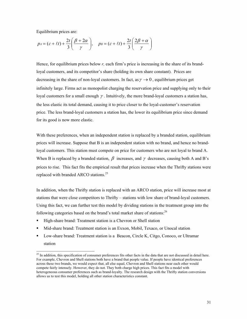
Equilibrium prices are:
+++=
γαβ 2
32)( ttcpA l ,
+++=
γαβ2
32)( ttcpB l
Hence, for equilibrium prices below r, each firm’s price is increasing in the share of its brand-
loyal customers, and its competitor’s share (holding its own share constant). Prices are
decreasing in the share of non-loyal customers. In fact, as 0→γ , equilibrium prices get
infinitely large. Firms act as monopolist charging the reservation price and supplying only to their
loyal customers for a small enough γ . Intuitively, the more brand-loyal customers a station has,
the less elastic its total demand, causing it to price closer to the loyal-customer’s reservation
price. The less brand-loyal customers a station has, the lower its equilibrium price since demand
for its good is now more elastic.
With these preferences, when an independent station is replaced by a branded station, equilibrium
prices will increase. Suppose that B is an independent station with no brand, and hence no brand-
loyal customers. This station must compete on price for customers who are not loyal to brand A.
When B is replaced by a branded station, β increases, and γ decreases, causing both A and B’s
prices to rise. This fact fits the empirical result that prices increase when the Thrifty stations were
replaced with branded ARCO stations.25
In addition, when the Thrifty station is replaced with an ARCO station, price will increase most at
stations that were close competitors to Thrifty – stations with low share of brand-loyal customers.
Using this fact, we can further test this model by dividing stations in the treatment group into the
following categories based on the brand’s total market share of stations:26
High-share brand: Treatment station is a Chevron or Shell station
Mid-share brand: Treatment station is an Exxon, Mobil, Texaco, or Unocal station
Low-share brand: Treatment station is a Beacon, Circle K, Citgo, Conoco, or Ultramar
station 25 In addition, this specification of consumer preferences fits other facts in the data that are not discussed in detail here. For example, Chevron and Shell stations both have a brand that people value. If people have identical preferences across these two brands, we would expect that, all else equal, Chevron and Shell stations near each other would compete fairly intensely. However, they do not. They both charge high prices. This fact fits a model with heterogeneous consumer preferences such as brand-loyalty. The research design with the Thrifty station conversions allows us to test this model, holding all other station characteristics constant.

32
Table VIII presents results from the fixed-effects regression where the treatment group is divided
into four groups: the effect of an Independent on stations in High-share, Middle-share, Low-
share, and ARCO categories.
Table VIII: Fixed-Effects Estimation, Independent coefficient by Brand Group Dependent Variable: Retail Price for Regular Unleaded (Standard Errors in Parentheses) Variable Parameter Estimate P-Value Intercept 1.3622
(0.0287) 0.0001
Company Operated -0.0018 (0.0124)
0.8842
Independent: High-share Brands -0.0304 (0.0127)
0.0168
Independent: Middle-share Brands -0.0447 (0.0143)
0.0018
Independent: Low-share Brands
-0.0707 (0.0185)
0.0001
Independent: ARCO
-0.0743 (0.0149)
0.0001
LA*February 0.0185 (0.0037)
0.0001
LA*June 0.0249 (0.0036)
0.0001
LA*October 0.1390 (0.0036)
0.0001
SD*February -0.0854 0.0066
0.0001
SD*June -0.0303 (0.0065)
0.0001
SD*October 0.0542 (0.0064)
0.0001
Adj. R-Square 0.7183
The brands are grouped in categories, since there are not enough stations in the treatment group
for some of the brands to allow for precise estimation of the effects of Independents on each
brand. For some brands with larger representation, such as Chevron and Shell, or Texaco and
Mobil, their coefficients are similar when included separately, however, grouping them improves
the precision of the estimates. In addition, the percent of each brand present in the treatment
group approximately reflects the percent of each brand in the station population, adding evidence
that the Thrifty chain was fairly evenly distributed among different brand competitors.
26 These brand categories also roughly follow market presence. Chevron and Shell each have 15-20% of the stations in each metropolitan area. Low brands have only a handful of stations, and the middle brands have market shares of 5-11%.

33
An F test shows that the coefficient on High-share Brands is significantly lower in absolute value
than the coefficient on Low-share Brands, with an F value of 4.13, which is significant at the 5
percent level. However the coefficient on Low-share Brands is not statistically different from the
coefficient on Middle-share Brands, nor is the coefficient on Middle-share Brands significantly
different from the coefficient on High-share Brands. However, the patterns lend some further
evidence supporting a model of product differentiation with brand-loyalty since the spot estimates
are consistent with the hypothesis that stations with low market share compete more intensely
with unbranded stations for non-loyal customers than do stations with high market share and high
brand loyalty.
VIII. Conclusions
This study used exogenous shocks to a panel of retail stations in Los Angeles and San Diego to
determine and differentiate between the effects of the market share of company-op stations and
independent stations on retail prices. The research design based on the conversions of
independent Thrifty stations to ARCO stations and unique, detailed station-level data allow for
convincing estimation of these effects. The analysis finds that an increase in company-op stations
in a market does not lead to an increase in the retail price level relative to unaffected markets.
However, the loss of an independent station does have a significant positive impact on the retail
price. This finding is logical. Independent retailers are the only retailers that can purchase
gasoline from the lowest price wholesaler, and they are also the only stations that can completely
determine their retail price independently of the upstream refiner. Even though lessee dealers and
branded dealers can set the retail price, because the branded refiner can set the wholesale price
(specific to the station in the case of the lessee dealer) they effectively set the lowest retail price
that the station can charge. In the case of the lessee dealer, the refiner can set the lease rate, a
volume discount, and the station-specific dealer tank-wagon price. These may be sufficient tools
for retail price setting, as is evidenced in Shepard (1993).
The independent station is the only type of station that can purchase gasoline from any refiner and
independently set its retail markup, thus increasing competition at the wholesale and retail levels.
These results have important implications for legislation aimed at lowering retail gasoline prices
through the regulation of refiner-retailer contracts. The research design and detailed data also
allowed for inference on the underlying structure of retail price competition. Results indicate that
independent competitors have a significant negative impact on retail prices. The results are

34
consistent with a model of differentiated products where consumers have heterogeneous brand-
loyalty. When independents are replaced by branded integrated stations, competitors respond by
increasing prices.

35
Bibliography Barron John M. and John R. Umbeck “The Effects of Different Contractual Arrangements: The Case of Retail Gasoline Markets” Journal of Law and Economics, Vol. 27 (October 1984) pp. 313-329. Borenstein, Severin “Selling Costs and Switching Costs: Explaining Retail Gasoline Margins” RAND Journal of Economics, Vol. 22 no. 3 (Autumn 1991) pp. 354-369. Borenstein, Severin and Andrea Shepard ``Sticky Prices, Inventories, and Market Power in Wholesale Gasoline Markets.'' National Bureau of Economic Research Working Paper #5468, 1996b. Borenstein, Severin and Andrea Shepard “Dynamic Pricing in Retail Gasoline Markets.” RAND Journal of Economics, Vol. 27 no. 3 (Autumn 1996) pp.429-251. Borenstein, Severin Colin Cameron and Richard Gilbert “Do Gasoline Prices Respond Asymmetrically to Crude Oil price Changes?” Quarterly Journal of Economics, February 1997 pp. 306-339. Borenstein, Severin and Richard Gilbert “Uncle Sam at the Gas Pump: Causes and Consequences of Regulating Gasoline Distribution.” Regulation, Spring 1993 pp. 63-75. Diamond, Peter “A Model of Price Adjustment”, Journal of Economic Theory, June 1971, 3, pp. 156-168. Karrenbrock, Jeffrey D. “The Behavior of Retail Gasoline Prices: Symmetric or Not?” Federal Reserve Bank of St. Lewis Review, Vol. 73 (July/August 1991) pp.19-29. Klemperer, Paul “The Competitiveness of Markets with Switching Costs,” The Rand Journal of Economics, Vol. 18 no. 1 (Spring 1987) pp. 138-150. Rey, Patrick and Joseph E. Stiglitz “The Role of Exclusive Territories in Producers' Competition,” Rand Journal of Economics, Vol. 26, n3 (Autumn 1995) pp. 431-451. Salop, Steven C. and Joseph E. Stiglitz “Bargains and Ripoffs: A Model of Monopolistically Competitive Price Deispersion,” Review of Economic Studies, Vol. 44 (October 1977) pp. 493-510. Shaked, A. and Sutton J. “Multiproduct Firms and Market Structure,” Rand Journal of Economics, Vol. 21 (Spring 1990) pp. 45-62. Shepard, Andrea “Contractual Form, Retail Price, and Asset Characteristics.” RAND Journal of Economics, Vol. 24 no. 1 (Spring 1993) pp. 58-77. Shepard, Andrea "Pricing Behavior and Contracts in Retail Markets" American Economic Review, Vol. 80 no. 2 (May 1990) pp.427-431. Shepard, Andrea "Price Discrimination and Retail Configuration" Journal of Political Economy, Vol. 99 no. 1 (February 1991) pp. 30-53. Shepard, Andrea "Contractual Form, Retail Price, and Asset Characteristics in Gasoline Retailing." Rand Journal of Economics, Vol. 24 no. 1 (Spring1993) pp.58-77. Slade, Margaret E. “Exogeneity Tests of Market Boundaries Applied to Petroleum Products.” Journal of Industrial Economics, Vol. 34 no. 3 (March 1986) pp. 291-303. Slade, Margaret E. “Conjectures, Firm Characteristics, and Market Structure: An Empirical Assessment.” International Journal of Industrial Organization, Vol. 4 no. 4 (December 1986) pp. 347-369.

36
Slade, Margaret E. “Interfirm Rivalry in a Repeated Game: An Empirical Test of Tacit Collusion.” Journal of Industrial Economics, Vol. 35 no. 4 (June 1987) pp.499-515. Slade, Margaret E. “Vancouver's Gasoline-Price Wars: An Empirical Exercise in Uncovering Supergame Strategies.” Review of Economic Studies, Vol. 59 no. 2 (April 1992) pp. 257-76. Slade, Margaret E. “Empirical Games: The Oligopoly Case.” Canadian Journal of Economics, Vol. 28 no. 2 (May 1995) pp. 368-402. Slade, Margaret E. “Multitask Agency and Contract Choice: An Empirical Exploration.” International Economic Review, Vol. 37 no. 2 (May 1996) pp. 465-486. Slade, Margaret E. “Strategic Motives fro Vertical Separation: Evidence from Retail Gasoline Markets” Journal of Law, Economics, and Organization, Vol. 14 no. 1 (April 1998) pp. 84-113. Stahl, Dale O. II “Oligopolistic Pricing with Sequential Consumer Search.” The American Economic Review, Vol. 79 no. 4 (September 1989) pp. 700-712. Stiglitz, Joseph E. “Equilibrium in Product Markets with Imperfect Information.” The American Economic Review, Vol. 69 (May 1979) pp. 339-345. Tirole, Jean The Theory of Industrial Organization, The MIT Press: Cambridge, Massachusetts, 1988. Varian, Hal R. “A Model of Sales.” The American Economic Review, Vol. 70 (September 1980) pp. 651-659. “California Refiners Face Hurdle in Federal, State RFG Rules.” Oil and Gas Journal, October 10, 1994. PennWell Publishers, Inc. “Deadline Looming for California Refiners to Supply Phase II RFG.” Oil and Gas Journal, December 11, 1995. PennWell Publishers, Inc. “A Statistical Analysis of the Lundberg Price Survey of selected Arizona Retail Petroleum Markets" by John Umbeck and Jack Barron, Study for WSPA.
Office of the Attorney General: Attorney General’s Report on Competition in Arizona’s Gasoline Prices, January 1998. “An Analysis of Arizona Gasoline Markets: October 1997”, R. Mark Isaac, Ronald L. Oaxaca, and Stanley S. Reynolds, for WSPA.
”The Cause and Effect of Divorcement/Fair Wholesale Supply Ordinance Proposed by Local Government in San Diego County”, by Tim Hamilton, AUTO Washington.
“Arizona’s High Gasoline Prices and the Benefits of Combining Retail Divorcement with a Prohibition Against Price Discrimination”, by Tim Hamilton, AUTO Washington.
37
Appendix
I. Retail Market Definitions
The variance components estimation indicates that there is significant variation in retail gasoline
prices within sub-city regions. This implies that competition occurs between stations in smaller
geographic regions with in each sub-city. Retail dealers and refiners state that these competition
groups have quite narrow geographic definitions. The one mile definition of competition groups
was adopted for the main results presented in the paper, and this section explores how these
results are affected by changes in this definition, and what this implies for competition in retail
markets. A rigorous economic exploration of the determinants of retail gasoline market
definitions is the topic of further research.
Dealers state that geographic competition is fairly narrowly defined. Although there is some spill-
over, dealers claim that they compete mostly with stations within a mile. “Compete with” in this
case means that if the competitor lowers his price, for example, by three cents a gallon, then the
dealer will notice a drop in his volume demanded. This definition is further reinforced by the fact
that stations of the same brand are located more than a mile apart (see Graph III). Even along the
same street, it is fairly common to find stations of the same brand, but they are almost always at
least a mile apart. In addition, many contracts between branded dealers and branded refiners
stipulate that the refiner will not brand another station within one mile of that dealer’s location.27
In order to illustrate the relationships between competition intensity and station location,
Fullerton is used as a representative sub-city in the Los Angeles metropolitan area. Graph II
shows a map of this example. The stations with price observations are labeled on the example
map. These comprise roughly 25 percent of the stations in this area. In Fullerton, the Beacon
station, and the ARCO and Chevron stations are included in the treatment group, since they are
within a mile away from the Thrifty station that was converted to an ARCO station. Applying this
definition to the whole sample of stations in Los Angeles and San Diego yields the results
presented earlier in the paper.
27 Barron and Umbeck (1984) ask refiners to list stations that they believe compete with stations in their data sample. The refiners list 3-4 stations as competitors for each station, and the authors use these groups as market definitions. Again, the market is defined narrowly: 3-4 stations usually fall within a mile of eachother. Also, Virginia's divorcement legislation required that a one and a half mile distance between any new company-op station and an existing dealer.

38
Suppose that the definitions are broadened by half a mile so that the stations compete with any
station within one-and-a-half miles. This definition will now include more stations in the
treatment group: stations that competed with an independent station that became a branded station
of any contractual type. This now implies that ARCO station at 401 N. Placentia Avenue is in the
treatment group. When this geographic definition change is applied to the whole sample of
stations in the Los Angeles and San Diego metropolitan areas, the results of the paper are not
significantly affected.
Table A.I: Fixed-Effect Estimation with Market Definition at One and a Half Miles Dependent Variable: Retail Price for Regular Unleaded Gasoline Variable Parameter
Estimate T-Statistic Standard
Deviation P-Value
Intercept 1.3599 47.5736 0.0285 0.0001 Company Operated 0.0023 0.2306 0.0102 0.8176 Independent -0.0444 5.5611 0.0087 0.0001 LA*February 0.0180 8.5576 0.0036 0.0001 LA*June 0.0243 4.9583 0.0036 0.0001 LA*October 0.1389 39.0635 0.0035 0.0001 SD*February -0.08512 -13.037 0.0066 0.0001 SD*June -0.0304 -4.6878 0.0065 0.0001 SD*October 0.0545 8.5576 0.0063 0.0001 Adjusted R-Square 0.7201 F-Test for No Fixed Effects: Numerator DF: 668 Denominator DF: 1999 F value: 3.2855
Prob. > F: 0.000 Hausman's M Value: 622.2957 Prob. > M: 0.000
Further increasing the scope of competition would expand the bounds of geographic competition
to 2 miles along streets and cross streets. In the Fullerton example, the treatment group is
unchanged, since there are no stations that are further than 1.5 miles, but closer than 2 miles.
Other markets are affected by this change, however. If this definition is applied to the whole
sample, then the estimate of the effect of an independent competitor on a station’s own price
drops to –3.61 cents per gallon, indicating that adding these stations brings the mean change in
price of the treatment group closer to that of the control group. This estimate is significantly
different that the initial estimate of –5 cents at the 95% confidence level. This indicates that
including these station lowers the average treatment effect, however the coefficient on
Independent is still relatively large and significantly different than zero. Even if market
definitions are increased by 100% of the industry definition, the result is still significant.

39
Table A.II: Fixed-Effect Estimation with Market Definition Two Miles Dependent Variable: Retail Price for Regular Unleaded Gasoline Variable Parameter
Estimate T-Statistic Standard
Deviation P-Value
Intercept 1.3787 47.537 0.0290 0.0001 Company Operated -0.0071 -0.7709 0.0092 0.4408 Independent -0.0361 -4.4406 0.0081 0.0001 LA*February 0.0194 5.1504 0.0037 0.0001 LA*June 0.0256 6.8631 0.0037 0.0001 LA*October 0.1389 38.886 0.0035 0.0001 SD*February -0.0827 -12.2679 0.0067 0.0001 SD*June -0.0288 -4.3585 0.0066 0.0001 SD*October 0.0545 8.5188 0.0064 0.0001 Adjusted R-Square 0.7155 F-Test for No Fixed Effects: Numerator DF: 668 Denominator DF: 1999 F value: 3.2054
Prob. > F: 0.000 Hausuman's M Value: 629.1963 Prob. > M: 0.000
One more increase can be made before reaching the sub-city level. The final group increases the
market definitions out to 3 miles along streets. Industry evidence suggests that stations in such a
large geographic range do not compete directly with each other. There are geographically
differentiated markets within this range, and therefore the treatment group will include stations
that did not directly compete with the affected Thrifty stations. In the Fullerton example, the Shell
and station will now be included in the treatment group. Applying this definition to the entire
sample lowers the average treatment effect further, however it is still significantly different than
zero.
Past three miles, the competition groups are equivalent to the sub-city definition used in the
variance of components estimation presented earlier, for most sub-cities in the sample. In fact, in
the case of Fullerton, the 3 mile definition includes all but one of the price observation stations in
the sub-city sample. At the next level, the sub-city level, there is a significant variation that is not
being controlled for. There is significant evidence that the first definition is the correct model of
local competition, however increasing this definition by 50% does not significantly change the
results.

40
Table A.III: Fixed-Effect Estimation with Market Definition Three Miles Dependent Variable: Retail Price for Regular Unleaded Gasoline Variable Parameter
Estimate T-Statistic Standard
Deviation P-Value
Intercept 1.3729 47.1558 0.0290 0.0001 Company Operated -0.0008 -0.1022 0.0092 0.9186 Independent -0.0220 -2.8844 0.0081 0.0040 LA*February 0.0179 4.7027 0.0037 0.0001 LA*June 0.0244 6.4533 0.0037 0.0001 LA*October 0.1389 38.6995 0.0035 0.0001 SD*February -0.0851 -12.3840 0.0067 0.0001 SD*June -0.0309 -4.6131 0.0066 0.0001 SD*October 0.0545 8.4778 0.0064 0.0001 Adjusted R-Square 0.7181 F-Test for No Fixed Effects: Numerator DF: 668 Denominator DF: 1999 F value: 3.262
Prob. > F: 0.000 Hausman's M Value: 622.2957 Prob. > M: 0.000
II. Probit Estimation of Contract Choice
A Probit regression of ARCO’s choice for dealer-run versus company-op contracts on station and
demographic characteristics is presented in Table A.IV. The assignment of a Dealer Contract is
given a value of one, so the table below shows the influence of each covariate on the probability
that a Thrifty station received a Dealer-run contract.
Table A.IV shows that Income, Percent White, and Number of Competitors were insignificant
explanatory variables of the assignment of contract type at the new ARCO stations. Even though
Percent White was significantly positively correlated with higher prices in the pooled regression
analysis in Table IV, it is not a significant determinant of ARCO's contract decisions. Number of
Competitors within a mile was negatively correlated with prices in the pooled regression,
however it is also not a significant determinant of contract choice. Several factors that may affect
the degree of local market competition were also included. The percent of competitors that are
dealers, the refiner concentration (HHI), and the distance to the nearest competitor were all
included as regressors. None of these factors were significant determinants of ARCO's contract
decision.

41
Table A.IV: Probit Estimation of the Probability of Choosing a Dealer Contract Type
Variable Parameter Estimate
Standard Error Chi Square Probability>Chi
Intercept -0.2718 1.9811 0.0188 0.0891 Existing Arco Dealer within 1 mile
0.6579 0.2640 6.2096 0.0127
HHI 0.5357 0.8227 0.0424 0.5149 Number of Competitors -0.0040 0.1062 0.0014 0.9699 Percent of Competitors with Dealer contracts
0.1945 0.3213 0.3664 0.5450
Distance to Nearest Competitor
-0.00008 0.0001 0.3830 0.5360
Ave. Quantity Food 0.000009 0.00001 0.6448 0.4220 ATM machine -0.7505 0.4638 2.618 0.1056 Convenience Store Size 0.2892 0.2280 1.4579 0.2273 Service Bay -0.4143 0.4201 0.9727 0.3240 Credit Cards Accepted 0.5498 0.2406 5.2225 0.0223 No. Self-serve Nozzles -0.0172 0.0201 0.7321 0.3922 Per Capita Income 0.000004 0.00002 0.0480 0.8266 Percent White 0.7359 0.8167 0.8119 0.3676 Percent of Workers Commuting Alone
-0.1492 2.2951 0.0042 0.9481
Average Commute Time 0.0094 0.0278 0.1151 0.7344 Percent of Workers using Public Transportation
-0.5884 2.9304 0.0403 0.8409
N = 170 Log Likelihood:
-92.74
Only two variables were significant determinants of contract type: whether the Thrifty station was
located within a mile of an existing ARCO dealer-run station, and whether the Thrifty station
accepted credit cards. Both of these factors increased the probability that the station was assigned
a Dealer contract instead of a Company-op contract. ARCO claimed that they preferred a dealer
contract if the station was too close to an existing ARCO dealer. This abated the chances that the
existing ARCO dealer would protest the branding of the new station. Dealers are much more
likely to protest if they are forced to compete with a station directly operated by their refiner, than
with one operated by another dealer. ARCO also claimed that they preferred to assign a dealer
contract if a "competitive" and "conscientious" dealer was available. Since Thrifty did not have a
policy of accepting credit cards, the decision to accept credit cards was left to the dealer. Since
merchants must pay the credit card processing fees, this acceptance of credit cards may indicate
the presence of a "competitive" dealer, especially since major branded competitors usually accept
credit cards.

Graph III: Map of Thrifty Stations in Los Angeles Metropolitan Area. Squares with flags denote a Thrifty Station

43
Graph IV: Sample Thrifty Conversion in Fullerton. The flag denotes a Thrifty station that was converted to an ARCO station. The boxes mark the locations of stations with price observations.

44
Graph V: Sample of stations in La Habra, California in the Los Angeles Metropolitan Area Census Data from La Habra shows the distance between stations of the same brand. 1 mile = | |