How vertical relationships and external funding a¤ect investmente¢ ciency and timing?

Dimitrios Zormpas�

March 21, 2017

AbstractIn this paper we consider a potential investor who contemplates entering an uncertain new

market under two conditions: i) a prerequisite for the project to take place is the purchaseof a discrete input from an upstream �rm with market power and ii) the completion of theinvestment is conditional on the participation of an investment partner who is willing to bearsome of the investment cost receiving compensation in return.Using the real option approach, we �nd that the involvement of any of the two alien agents

causes the postponement of the completion of the investment and we discuss how these timingdiscrepancies are re�ected on the value of the option to invest in the project. We next analyzethe synchronous e¤ect of outsourcing and external funding both in a non-cooperative and in acooperative (Nash bargaining solution) game-theoretic setting and we show how the endogeneityof the sunk investment cost a¤ects the timing and the value of the option to invest in projectscharacterized by uncertainty and irreversibility.keywords: Investment analysis, Real options, Vertical relations, Nash bargaining solution.jel classification: C61, D92, G30.

1 Introduction

Innovation is an important factor for a company�s success and a crucial explanation for observeddi¤erentials in performance (McGrath and Nerkar, 2004). Consequently, a fundamental problemthat a �rm faces has to do with the decision to invest in a new product, technology or servicemarket. These kinds of managerial decisions are usually characterized by risky, irreversible andlumpy investments that are often beyond the resources of a single �rm (Chesbrough and Schwartz,2007) and, as a result, an investment partner willing to share the cost of betting on the successof the business plan under consideration is frequently sought after (Kogut, 1991). According toQuinn (2000), using partnerships �companies have lowered innovation costs and risks by 60% to90%, while similarly decreasing cycle time and leveraging their internal investments by tens tohundreds of times�.

Investment partnerships might take the form of joint ventures, independent or corporate venturecapital investments, strategic alliances or merges. Irrespective of the exact nature of the partner-ship, the underlying reasons that motivate it are common. When joining forces with another �rm,an investment partner anticipates �nancial returns and/or a window on new technologies that cor-respond to future growth opportunities.1 As noted by Miller and Modigliani (1961), a signi�cant

�Department of Civil, Architectural and Environmental Engineering, University of Padova, Via Marzolo 9, 35131,Padova, Italy. Email: dimitrios.zormpas@studenti.unipd.it. Special thanks to Michele Moretto and Luca Di Coratofor valuable comments and suggestions.

1See e.g. Vrande and Vanhaverbeke (2013), Dushnitsky and Lenox (2005a) and Reuer and Tong (2007).

1

part of many �rms�market values consists of such future growth opportunities i.e. assets not yet inplace. Myers (1977) argued that these assets are analogous to �nancial options, in the sense thatone has the right but not the obligation to invest, and consequently stock option pricing methodsshould be used for their evaluation.

The real option approach acknowledges that investment opportunities are options on real assetsand provides a way to apply option pricing methods to investment decision problems. It claimsthat the classic net present value rule is not always valid and argues that the option to postpone aninvestment decision characterized by uncertainty and irreversibility has to be taken into account.McDonald and Siegel (1986) gave an expression for the option value and showed that the optimalinvestment strategy is a trigger strategy in the sense that one should invest as soon as the projectvalue is greater than a threshold, the value of which increases with uncertainty.2

In this paper we use the real option approach in order to describe the interaction among i) a�rm who is contemplating entering an uncertain new market, ii) a �rm who acts like an investmentpartner partly �nancing this project receiving a share of the �nal investment in return and iii)an upstream supplier with market power who is responsible for the provision of an input thatis necessary for the potential investor to start producing and selling. Using a stochastic dynamicprogramming model, we examine how the involvement of the two alien agents a¤ects the investmenttiming and how the observed timing discrepancies are re�ected on the value of the option toinvest. We show that both external funding and input outsourcing cause the postponement ofthe investment and we demonstrate how this erodes the project�s option value. Comparing thetwo e¤ects we �nd that external funding is preferred to input outsourcing, in the sense that thedistortion with respect to the optimal, vertically integrated, case is more limited. We then focus onthe three-agent case where the synchronous e¤ect of outsourcing and external funding is discussed.Using a non-cooperative game-theoretic framework we show that, as expected, this represents theworst-case scenario since we have the investment timing reaching its maximum and, consequently,the value of the option to invest reaching its minimum. In the concluding part of the paper weapproach the problem anew replacing the original non-cooperative game-theoretic setting with aNash bargaining solution. Given a set of participation conditions, we show that the presence of thetwo alien agents is still a¤ecting the investment timing. However, in this case the two e¤ects areopposing each other. Outsourcing is still causing the postponement of the project but now externalfunding is favoring the (ine¢ cient) acceleration of the investment. A comparison between the twoshows that the �rst force is always prevailing, a result that highlights the importance of the natureof the sunk investment cost when investment partnerships are considered.

The remainder of the paper is organized as follows. In Section 2 we provide a brief overviewof the related literature. In Section 3 we present in detail the model set-up demonstrating theconnection with previous work and in Section 4 we discuss the three-agent case. In Section 5 wesolve the problem under Nash bargaining and Section 6 concludes.

2 Literature review

This work relies on an established body of papers that integrate two research streams: the basictheory of irreversible investment under uncertainty as in Dixit and Pindyck (1994), and the classicpresentation of vertical relationships as described e.g. by Tirole (1988).3 Real option analysis hasbeen used to study joint ventures (Kogut, 1991; Li et al., 2008; Cvitanic et al., 2011; Banerjee et

2See e.g. Dixit and Pindyck (1994).3Recent overviews of the related literature include Chevalier-Roignant et al., 2011; Azevedo and Paxson, 2014;

Guimarães Dias and Teixeira, 2010; Huisman et al., 2004.

2

al., 2014), R&D and technology development (McGrath and Nerkar, 2004; McGrath, 1997; Folta,1998), outsourcing (Alvarez and Stenbacka, 2007; Kogut and Kulatilaka, 1994; Moretto and Rossini,2012; Di Corato et al., 2017; Triantis and Hodder, 1990; Teixeira, 2014), as well as venture capitalinvestments (Lukas et al., 2016; Vrande and Vanhaverbeke, 2013; Dushnitsky and Lenox, 2005b)and acquisitions (Folta and Miller, 2002; Benson and Ziedonis, 2009; Lambrecht, 2004; Tong andLi, 2011).

The most closely related work we have identi�ed is in corporate �nance and supply chainmanagement, most notably Lambrecht (2004), Banerjee et al. (2014) and Chen (2012), Lukas andWelling (2014).

Lambrecht (2004) analyzes a merger between two �rms motivated by economies of scale usingtwo di¤erent sequences of moves. According to the �rst (friendly merger), one of the two partiesis choosing the optimal timing and then the terms of the merger are commonly decided, whereas,according to the second (hostile takeover), the two parties commit to the terms of the merger �rstand the timing is decided second. A comparison between the two suggests that, the way synergiesare divided may in�uence the timing of the merger. Similarly, Banerjee et al. (2014) use a two-stagedecision-making framework in which the parties determine the sharing rule as an outcome of Nashbargaining and one of them makes the timing decision related to the exercise of the jointly heldoption. Considering both cash transfers and ownership stakes, they show that when the exercisedecision is made �rst, timing is always optimal4 whereas, when the sharing rule is determined�rst (hostile takeover case from Lambrecht, 2004) investment timing is socially ine¢ cient unless acombination of stake in the project and a cash transfer is used. In this case, it generally matterswhich �rm makes the timing decision and how the bargaining power is distributed.

In the supply chain management literature, Chen (2012) models a two-echelon supply chainconsisting of one supplier and one retailer. The two-stage optimization problem evolves in thefollowing way. In the �rst stage, the two agents negotiate over the optimal quantities whereas inthe second stage, they coordinately determine the optimal timing of investing in the supply chainunder uncertain demand. The results show that the volatility of demand shock has an ambiguouse¤ect on the investment threshold with increasing impacts at lower level and decreasing impacts athigher level of uncertainty. Lastly, Lukas and Welling (2014) model the optimal timing of "climate-friendly" investments in a supply chain framework and enrich the contribution of Chen (2012) inthe following ways. Firstly, they adopt a non-cooperative real option game setting according towhich the optimal timing is decided, not jointly but by one of the participating �rms and, secondly,they extend the two-echelon supply chain allowing for more than two participants showing that asupply chain becomes less e¢ cient with every additional link as the timing distortion builds up.

In spite of the di¤erences in their analyses, what all these papers have in common is the natureof the investment cost which is tacitly assumed to be exogenous. As Billette de Villemeur et al.(2014) point out, this assumption seems reasonable when the investment is performed largely in-house, as may occur with R&D, but this is not always the case. For instance, there are many othercases in which the completion of a �rm�s investment project depends on an upstream supplier who isresponsible for the provision of a discrete input. In that case, the cost of the single �rm�s investmentis endogenous since it is speci�ed by the vertical relationship between the external supplier and thepotential investor.

The novelty of our work lies on the fact that the investment cost is explicitly assumed to beendogenous. We begin by analyzing a non-cooperative game-theoretic setting according to which,the optimal timing is decided by the investment partner whereas the sharing rule is decided by the

4This is a generalization of the friendly merger case discussed in Lambrecht (2004) and in Morellec and Zhdanov(2005).

3

project originator, given the price of an indispensable input provided by an external supplier withmarket power. We subsequently readdress this three-agent5 problem deriving the conditions underwhich it would be socially preferable to determine the sharing rule as an outcome of Nash bargainingand we �nd that the presence of the upstream �rm makes a substantial di¤erence when we considerthe timing and the value of the option to invest in a given project, both in the cooperative (Nashbargaining solution) and in the non-cooperative case.

3 The model

3.1 The basic set-up

Firm A is a risk neutral potential investor willing to enter a market with growing but uncertaindemand. The pro�t �ow that A is cashing upon investment is yt�M where �M > 0 is the instan-taneous monopolistic pro�t per unit of yt and yt is a stochastic scale parameter that �uctuatesaccording to the following geometric Brownian motion:

dytyt= �dt+ �dWt, y0 = y, (1)

where � > 0 is the drift, � > 0 is the instantaneous volatility and dWt is the standard increment ofa Wiener process (standard Brownian motion) uncorrelated over time satisfying E [dWt] = 0 andE�dW 2

t

�= dt.

A discrete input is a prerequisite for A to operate in the �nal market and this input is suppliedby an upstream �rm with market power that we call C. It is assumed that C prices this inputtaking into consideration the structural parameters of the geometric Brownian motion presentedabove, but without ever observing yt.6

The completion of the project depends also on the cooperation of an investment partner B whois willing to bear a share of the investment cost, asking for compensation in return. Contrary tothe upstream �rm, we assume that the investment partner is in a position to continuously andveri�ably observe the �uctuations of the scale parameter over time. One can argue that this is asensible assumption since B will consider joining forces with A only if s/he has enough informationfor the considered project. For instance, we can think of B as a �nancial institution and A as acustomer asking for a business loan. The customer will need to present a thorough business planin order to convince the �nancial institution about the promising character of the project. In thiscase, the potential investor is basically voluntarily sharing her/his information endowment withthe investment partner. Alternatively, one can assume that B might actually be in a position toobserve the scale parameter over time without A�s help. For instance, Mulherin and Boone (2000)as well as Vrande and Vanhaverbeke (2013) report evidence for signi�cant industry clustering formerger and acquisition activities. These �ndings support the argumentation from Puranam et al.(2009) and Dushnitsky and Lenox (2005b) who suggest that �rms seem to seek ventures similar to

5Note that our framework involves three agents of di¤erent type: the project originator, the investment partnerand the input supplier. It is true that models with more than two agents have already been analyzed in the literature.For instance, Billette de Villemeur et al. (2014) present the case of a downstream duopoly with an upstream supplierand Banerjee et al. (2014) extend their two-party model to any number of investment partners. However, in bothcases, as well as in the N-echelon supply chain presented by Lukas and Welling (2014), the types of agents are alwaystwo. The introduction of a third type is the key originality of our framework.

6As noted by Billette de Villemeur et al. (2014), if C is in a position to continuously and veri�ably observethe state of yt, then s/he can expropriate the project by choosing a suitable input price. Here we assume that theupstream �rm has no access to this kind of information.

4

their own because this appears to facilitate the possible integration of technological resources inthe future.

Before analyzing the three-agent case where the interaction among A, B and C is discussed,we brie�y review the problem under (i) vertical integration and (ii) outsourcing or partial externalfunding (but not both).

3.2 Vertical Integration

The vertically integrated case will be our benchmark. In this simpli�ed setting it is assumed thatthe potential investor produces the input in-house funding privately the completion of the project.

Following the real option literature, we keep in mind that there is some �exibility when weconsider an investment opportunity under irreversibility and uncertainty. As �rstly reported byMcDonald and Siegel (1986), the ability to delay an irreversible investment expenditure is animportant source of �exibility that profoundly a¤ects the decision to invest. A will only invest whenthe project�s expected payo¤ exceeds the cost of the investment by the option value of waiting toinvest.7

Assuming that the initial market size is positive and su¢ ciently small so that a delay of theinvestment is preferable, the optimal investment time point �V I is derived through the solution ofthe following maximization problem:

F V IA (y) = max�V I

Ey

�(V�V I � I)e�r�

V I�= max

yV I

�yV I�Mr � a � I

��y

yV I

��; (2)

where Vt = Et�R1t ys�Me

�r(s�t)ds�= yt�M

r�a is the value of the project, � �12�

a�2+q�

a�2� 1

2

�2+ 2r

�2>

1 is the positive root of the characteristic equation 12�

2�(� � 1) + �� � r = 0, r (> �) is the com-mon to all �rms discount rate,8 I > 0 is the sunk cost of producing the input in-house and�V I = inf

�t � 0

��yt = yV Iis the random �rst time point that yt hits the barrier yV I which is the

market size that triggers the investment. The expressions for F V IA (y) and � are standard in the realoption literature (see Dixit and Pindyck (1994), Chapters 5-6 and Dixit (1993), Section 2). Fromthe �rst-order condition we have

yV I =�

� � 1r � ��M

I: (3)

As expected, yV I is increasing in the sunk investment cost I and the volatility � but is decreasingin the present value of the pro�t �ow �M

r�� .9 In words, a �rm stands to gain more by holding, rather

than exercising, an investment option with a high strike price (I in this case), a high underlyingasset volatility (� in this case) but small return ( �Mr�� in this case).

10

Combining Eq. (2) with Eq. (3) we obtain the value of the option to invest

F V IA (y) =I

� � 1

�y

yV I

��: (4)

These results lead to the �rst proposition:

7O�Brien et al. (2003) present strong empirical evidence in favor of this argument. More precisely, they �nd thatentrepreneurs account for the value of the option to delay entering a new market when contemplating such a decision.

8The inequality r > � guarantees convergence.9Note that the e¤ect of volatility on the investment threshold passes through �.10Note that the classic net present value rule would dictate the lower investment threshold yNPV = r��

�MI. As one

can see, even a risk neutral potential investor is sensitive to uncertainty when considering an irreversible investmentthe realization of which can be postponed for the future.

5

Proposition 1 A single �rm that produces the input in-house and self-�nances the investmentproject, will enter the market as soon as the scale parameter reaches a threshold yV I = �

��1r���M

I.

The value of the option to invest in this project is F V IA (y) = I��1

�yyV I

��.

3.3 The input is outsourced and the investment is privately funded

Suppose now that the input is produced by an upstream �rm with market power that we call C.Adopting the framework presented by Billette de Villemeur et al. (2014), we assume that A andC engage in a leader-follower game at time zero. Moving backwards, A (the follower) decides theoptimal investment threshold taking into consideration the constant input price p. Then, C (theleader) decides the optimal p accounting for the production cost I, the structural parameters of thestochastic term yt and A�s timing decision.

The optimal investment threshold is derived through the solution of the following maximizationproblem:

FOSA (y) = maxyOS(p)

�yOS(p)�Mr � a � p

��y

yOS(p)

��(5)

Solving we obtain

yOS(p) =�

� � 1r � ��M

p: (6)

The decision problem of C, involves only the choice of p that is derived as the solution of FOSC (y) =

maxpOS

�pOS � I

� � yyOS(pOS)

��. Solving we have

pOS =�

� � 1I: (7)

Combining the optimal investment trigger from Eq. (6) with the optimal input price from Eq. (7),we obtain yOS

�pOS

�= �

��1r���M

���1I which can be written as

yOS�pOS

�=

�

� � 1yV I�> yV I

�: (8)

From Eq. (7) and Eq. (8) one can see that both pOS and yOS�pOS

�are decreasing in � i.e. are

increasing in volatility. This implies that A will probably consider abandoning a very risky projector, in any case, will delay the investment as much as possible.11 C takes this into account settinga high pOS discounting this way for the delay between the time that pOS is chosen until the timeit is cashed. Similarly, a project that involves very little risk will be undertaken relatively quicklyby A and this will also be re�ected on a lower input price. Note however, that there is a minimumfor pOS : lim

�!0pOS = r

r�aI > I. As one can see, despite the fact that the acceleration of the project

is bene�cial for C, s/he is not willing to lower pOS below a minimum rr�aI. This has to do with

the fact that, for prices below rr�aI, the completion of the project is indeed further hastened but

what is sacri�ced in terms of cash �ow is not remunerated from the additional acceleration of theproject.

Combining Eq. (5), (7) and (8) we obtain

FOSA (y) =

�� � 1�

���1F V IA (y): (9)

11 lim�!1

yOS�pOS

�!1

6

Also, for C we have

FOSC (y) =

�� � 1�

��F V IA (y): (10)

The following proposition summarizes these �ndings:

Proposition 2 A single �rm that outsources the input and self-�nances the investment project,will enter the market as soon as the scale parameter reaches a threshold yOS

�pOS

�= �

��1yV I . The

value of the option to invest in this project is FOSA (y) =���1�

���1F V IA (y).

Comparing our �ndings from Propositions 1 and 2 we obtain the following:

Proposition 3 When an upstream supplier is responsible for the provision of the input, the in-vestment is postponed

�yOS > yV I

�and the potential investor�s option to invest is less valuable�

FOSA (y) < F V IA (y)�.

As one can see, the e¤ect of the presence of C is twofold. On one hand, it increases theinvestment threshold delaying the completion of the project and, on the other, it reduces the valueof the option to invest for the potential investor A.

3.4 The input is produced in-house and the investment is partly externallyfunded

Going back to the case of vertical integration, we assume that the potential investor produces theinput in-house. However, the realization of the project that A has in mind depends now on thecooperation of an investment partner B.

Following Lukas and Welling (2014), B is willing to undertake an exogenously given share� 2 (0; 1) of the sunk investment cost, and this allows A to fund only the rest of the project. Inreturn, A and B negotiate over the compensation that the former needs to pay to the latter. Moreprecisely, we assume that at time zero A credibly commits to o¤er a fraction 2 (0; 1) of theproject to B. Now B has the option to accept this o¤er immediately disbursing the capital neededfor the realization of the project or, alternatively, can delay this contribution for some future time.12

Similarly to the previous section, we have a leader-follower game with A (the leader) deciding thecompensation o¤er and B (the follower) deciding the optimal timing taking the compensation o¤er into account.13

Starting with the problem of the follower we have F V CB (y) = maxyV C( )

� yV C( )�M

r�a � �I��

yyV C( )

��.

Solving we obtain

yV C( ) =�

yV I : (11)

12As one can see, the adopted framework is general enough to describe joint ventures and independent venturecapital investments. However, it seems particularly suitable to describe corporate venture capital (CVC) investments.According to Roberts and Berry (1985), CVC investments consist of minority equity stakes in relatively new, notpublicly traded companies and their purpose is to identify and value early-stage technology in start-ups. Thisdescription corresponds exactly to the behavior of our investment partner B who agrees to receive a share of A�sproject instead of a standard cash �ow.13One can also consider the case where B is the game-leader submitting the compensation o¤er and A is the

game-follower deciding the investment timing. In Section A.1 of Appendix A we show that such a change does nota¤ect the nature of our main results.

7

As expected, yV C( ) is increasing in � and decreasing in . This just means that the investmentwill be postponed as the cost share for the investment partner is increasing, a result that can beneutralized if the potential investor is willing to improve the submitted compensation o¤er. As onecan see, A faces a dilemma since a low compensation o¤er implies access to a larger cash �ow laterin the future whereas a high compensation o¤er shortens the waiting period but gives access to asmaller cash �ow in return.

The potential investor takes into consideration the reaction of the investment partner anddecides the compensation o¤er that is derived as the solution of the following maximization problem:

F V CA (y) = max V C

��1� V C

� yV C( V C)�Mr � a � (1� �) I

��y

yV C( V C)

��, (12)

which yields

V C =� (� � 1)� � 1 + � : (13)

Combining Eq. (11) and Eq. (13) we obtain

yV C( V C) =� � 1 + �� � 1 yV I

�> yV I

�: (14)

Studying the optimal compensation o¤er, we can see that V C is increasing both in � and in �.Focusing on the e¤ect of �, it is interesting to see that the maximum optimal o¤er is always below100%. This has to do with the fact that a more generous compensation o¤er will indeed hasten thecompletion of the project but will only make the potential investor worse-o¤ since what is sacri�cedin terms of compensation is not remunerated from the acceleration of the investment.

One can also observe that yV C( V C) is increasing in � and decreasing in �. Actually, the"distance" between yV C( V C) and yV I increases in � despite the fact that, at the same time, V C

is also increasing in �. This happens because yV C( V C) is a linear, whereas V C is a concavefunction of �. In words, despite the fact that the compensation o¤er is becoming more generous asthe share of the cost covered by B increases, in real terms the o¤er worsens and this is re�ected ona higher investment threshold.

Lastly, combining Eq. (12), (13) and (14) we obtain

F V CA (y) =

�� � 1

� � 1 + �

���1F V IA (y): (15)

Also, for B we have

F V CB (y) = �

�� � 1

� � 1 + �

��F V IA (y): (16)

The following proposition summarizes these results.

Proposition 4 In the case where the single �rm produces the input in-house but the completionof the project depends on external funding, the investment occurs when the scale parameter reachesa threshold yV C( V C) = ��1+�

��1 yV I . The value of the option to invest in this project is F V CA (y) =���1��1+�

���1F V IA (y).

Comparing our �ndings with the values that we derived in the vertically integrated case wehave:

8

Proposition 5 In the case where the single �rm produces the input in-house but the completion ofthe project depends on external funding, the investment is delayed

�yV C > yV I

�and the potential

investor�s option to invest is less valuable�F V CA (y) < F V IA (y)

�.

As in Section 3.3, the e¤ect of the presence of the additional agent is twofold since, on one hand,it increases the investment threshold delaying the completion of the project and, on the other, itreduces the value of the option to invest for the potential investor.

4 The three-agent case

In this section we combine the analyses presented above and we show how the synchronous presenceof B and C a¤ects the performance and the actions of A as well as the investment threshold. Thethree-agent game evolves in the following way:

1. C is the game-leader and decides the input price that maximizes her/his value of the optionto invest.

2. Given the input price and the cost share �, A submits the compensation o¤er to B and,�nally,

3. B evaluates this compensation o¤er and decides when to accept it, disbursing the amountthat is required for the realization of A�s project.

Keeping in mind that A and B continuously and veri�ably observe the magnitude of yt whereasC only knows the structural parameters of the related stochastic process, we move backwards andwe �rst study the behavior of the investment partner B. The optimal investment threshold is

derived through the solution of: FB3(y) = maxy3( ;p)

� y3( ;p)�M

r�a � �p��

yy3( ;p)

��. Solving, we obtain

y3 ( ; p) =�

� � 1r � ��M

p�

: (17)

The potential investor A will take into consideration the decision of the investment partner andwill choose the compensation o¤er taking the price of the input as given. The optimal is derived

as the solution of FA3(y) = max 3

�(1� 3)

y3( 3;p)�Mr�a � (1� �) p

��y

y3( 3;p)

��. From the �rst-order

condition we have

3 =� (� � 1)� � 1 + � : (18)

As one can check, this is exactly the compensation o¤er that we derived in Eq. (13) where Cwas absent. Obviously, the presence/absence of C does not a¤ect the magnitude of the optimalcompensation o¤er that A submits to B since the exogenously given cost share � has to do withthe generic investment cost no matter if this is I or p.

We conclude with the game-leader C. The input supplier observes the behavior both of A and

of B and optimally decides the price of the input solving FC3(y) = maxp3(p3 � I)

�y

y3( 3;p3)

��which

yields:

p3 =�

� � 1I (19)

Comparing Eq. (19) with Eq. (7) we see that p3 = pOS which means that the presence/absence ofB does not a¤ect the optimal price of the input that is decided by C. This is not a surprise since,C is indi¤erent to the means that A uses to fund the project.

9

Combining Eq. (17), (18) and (19) we derive the investment threshold which, in this case, is

y3 ( 3; p3) =�

� � 1� � 1 + �� � 1 yV I

�> yV I

�: (20)

Note that y3 ( 3; p3) is decreasing in � and increasing in �. Similarly to yV C( V C), the "distance"

between y3 ( 3; p3) and yV I increases in � in spite of the simultaneous improvement of the corre-

sponding compensation o¤er. The reasoning is the same: the investment trigger is a linear whereasthe compensation o¤er is a concave function of the cost share �. As we have seen in the previoussection, despite the fact that the compensation o¤er is becoming more generous as the cost share� increases, in real terms the o¤er worsens and actually, in the three-agent case, this e¤ect is evenmore dramatic since the compensation o¤er worsens "faster" as the (positive) slope of y3 withrespect to � is larger than the (positive) slope of yV C with respect to � exactly because of thepresence of C.

We conclude this section returning to the option values for the three agents. Keeping in mindthe values for y3 ( 3; p3) ; p3 and 3 we obtain

FA3(y) =

�� � 1�

���1� � � 1� � 1 + �

���1F V IA (y); (21.1)

FB3(y) = �

�� � 1�

���1� � � 1� � 1 + �

��F V IA (y); (21.2)

FC3(y) =

�� � 1�

�� � � � 1� � 1 + �

��F V IA (y): (21.3)

The following proposition summarizes these results.

Proposition 6 In the three-agent case where the single �rm outsources the production of the inputand the completion of the project depends on external funding, the investment occurs when the scaleparameter reaches a threshold y3 ( 3; p3) =

���1

��1+���1 yV I . The value of the option to invest in this

project for the potential investor is FA3(y) =���1�

���1 ���1��1+�

���1F V IA (y).

Comparing our �ndings with the values that we derived in the vertically integrated case wehave:

Proposition 7 In the three agent case the investment takes place ine¢ ciently late�y3 ( 3; p3) > yV I

�and this is also re�ected on the potential investor�s option value

�FA3(y) < F V IA (y)

�.

4.1 Discussion

In the previous sections we focused on the e¤ect that the presence of additional agents has onthe investment threshold and the potential investor�s option value both for the two-agent and thethree-agent case. Keeping all this in mind we can examine this e¤ect in the level of the industryas a whole.

The input is outsourced and the investment is privately funded: We have already com-puted the value of the option to invest for the potential investor A and the input supplier C. Nowadding up Eq. (9) and Eq. (10) we obtain

FOS(y) � FOSA (y) + FOSC (y) =(� � 1)��1

��(2� � 1)F V IA (y): (22)

10

As one can see, the presence of the �rm C a¤ects negatively the value of the option to invest forthe whole industry since FOS(y) < F V IA (y).

The input is produced in-house and the investment is partly externally funded: Sum-ming Eq. (15) and Eq. (16) we obtain

F V C(y) � F V CA (y) + F V CB (y) =� � 1 + ��� � 1

�� � 1

� � 1 + �

��F V IA (y): (23)

The presence of �rm B a¤ects negatively the value of the option to invest for the whole industrysince F V C(y) < F V IA (y).

The three-agent case: Summing up the values of the option to invest for A, B and C from Eq.(21) we obtain

F3(y) � FA3(y) + FB3(y) + FC3(y) (24)

=

�� � 1�

���1� � � 1� � 1 + �

�� �� � 1 + �� � 1 + � +

� � 1�

�F V IA (y):

A comparison of the results derived in this and the previous sections is given in the followingproposition:

Proposition 8 A comparison among the investment triggers and the option values presented abovegives the following rankings:

1) y3 ( 3; p3) > yOS(pOS) > yV C( V C) > yV I ,2) F3(y) < FOS(y) < F V C(y) < F V IA (y),3) FA3(y) < FOSA (y) < F V CA (y) < F V IA (y),4) FB3(y) < F V CB (y) and5) FC3(y) < FOSC (y).

A number of interesting results can be derived by these comparisons. First of all, we see thatas the number of agents involved in an investment project increases, the completion of this projectis postponed to the detriment of the investment�s option value both in the �rm and in the industrylevel. As expected, the vertically integrated case represents the most favorable whereas the three-agent case represents the least favorable scenario. Another interesting observation has to do withthe comparison between the e¤ect of the presence of the upstream �rm C and the e¤ect of thepresence of the investment partner B. As we can see, external funding is preferred to outsourcingin terms of timing and, consequently, in terms of option value.14

4.2 Numerical Examples

We conclude this section using some numerical examples that will help us illustrate the e¤ect ofoutsourcing and external funding on the investment timing and the value of the option to enter thenew market.14 In Section A.2 of Appendix A we show that the ranking of the investment thresholds and, consequently, the

ranking of the aggregate option values, is the same even when A and B swap places i.e. if A becomes the time-deciding agent (game-follower) and B becomes the one that chooses the compensation share (game-leader). However,we also show that this is not the case for the ranking of A�s option values which is actually sensitive to such a change.

11

We assume that the parameters vary as follows: We let the drift, �, and the volatility, �, takevalues {0.025, 0.035} and {0.2, 0.25, 0.3, 0.35, 0.4} respectively. A high magnitude of the driftcaptures a high expected increase in the size of the new market whereas di¤erent levels of volatilityare used to demonstrate the impact of uncertainty on the investment thresholds and option values.The sunk investment cost I takes values {24, 48} whereas both the initial level of the stochasticparameter y0 and the instantaneous monopolistic pro�t per unit of yt, �M , are set equal to unity(y0 = �M = 1). We allow for three di¤erent levels of exogenous cost share: �1 = 0:1, �2 = 0:5 and�3 = 0:9 in order to demonstrate how the participation of an investment partner a¤ects the timingand the performance of the investment project. The interest rate r is initially set equal to 5% butwe also check the e¤ect of an increase to 6% which corresponds to a higher opportunity cost ofcapital.

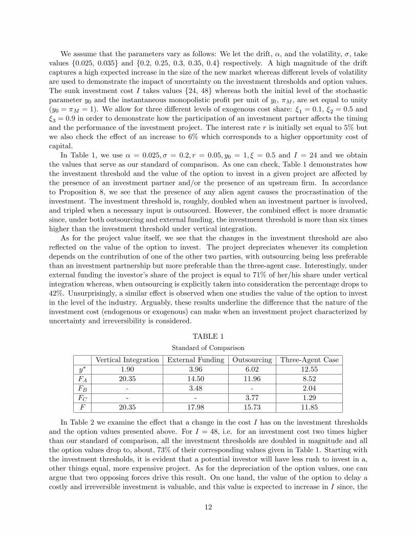
In Table 1, we use � = 0:025; � = 0:2; r = 0:05; y0 = 1; � = 0:5 and I = 24 and we obtainthe values that serve as our standard of comparison. As one can check, Table 1 demonstrates howthe investment threshold and the value of the option to invest in a given project are a¤ected bythe presence of an investment partner and/or the presence of an upstream �rm. In accordanceto Proposition 8, we see that the presence of any alien agent causes the procrastination of theinvestment. The investment threshold is, roughly, doubled when an investment partner is involved,and tripled when a necessary input is outsourced. However, the combined e¤ect is more dramaticsince, under both outsourcing and external funding, the investment threshold is more than six timeshigher than the investment threshold under vertical integration.

As for the project value itself, we see that the changes in the investment threshold are alsore�ected on the value of the option to invest. The project depreciates whenever its completiondepends on the contribution of one of the other two parties, with outsourcing being less preferablethan an investment partnership but more preferable than the three-agent case. Interestingly, underexternal funding the investor�s share of the project is equal to 71% of her/his share under verticalintegration whereas, when outsourcing is explicitly taken into consideration the percentage drops to42%. Unsurprisingly, a similar e¤ect is observed when one studies the value of the option to investin the level of the industry. Arguably, these results underline the di¤erence that the nature of theinvestment cost (endogenous or exogenous) can make when an investment project characterized byuncertainty and irreversibility is considered.

TABLE 1

Standard of Comparison

Vertical Integration External Funding Outsourcing Three-Agent Casey� 1.90 3.96 6.02 12.55FA 20.35 14.50 11.96 8.52FB - 3.48 - 2.04FC - - 3.77 1.29F 20.35 17.98 15.73 11.85

In Table 2 we examine the e¤ect that a change in the cost I has on the investment thresholdsand the option values presented above. For I = 48, i.e. for an investment cost two times higherthan our standard of comparison, all the investment thresholds are doubled in magnitude and allthe option values drop to, about, 73% of their corresponding values given in Table 1. Starting withthe investment thresholds, it is evident that a potential investor will have less rush to invest in a,other things equal, more expensive project. As for the depreciation of the option values, one canargue that two opposing forces drive this result. On one hand, the value of the option to delay acostly and irreversible investment is valuable, and this value is expected to increase in I since, the

12

more expensive the investment, the more valuable the option to postpone it. On the other handhowever, the higher investment threshold implies a further delay of the investment which eventuallydistances the anticipated cash �ow further in the future. As one can see, the second force prevails.

TABLE 2

The E¤ect of a Change in the Investment Cost on Timing and Option Value

I = 48

Vert. Integ. Ext. Funding Outsourcing Three-Agent Casey�=y�T1 2 2 2 2FA=F

T1A 0.73 0.73 0.73 0.73

FB=FT1B - 0.73 - 0.73

FC=FT1C - - 0.73 0.73

F=F T1 0.73 0.73 0.73 0.73

In Table 3, we study the e¤ect that changes in the drift, �, may have. A comparison of theoption values of Table 3 with the ones that we derived in Table 1 shows that an increase in theexpected growth rate from � = 0:025 to � = 0:035, is bene�cial both in the �rm and in theindustry level. However, the e¤ect of such a change in the investment triggers is not as obvious.Actually, we observe that a higher � is, ceteris paribus, encouraging the acceleration of a projectunder vertical integration but is causing the further postponement of projects the completion ofwhich is conditional on the participation of a second or a third party. Especially, in the three-agentcase, we see that a �� = 0:01 is enough to (more than) double the related investment threshold.The intuition behind this result has to do exactly with the absence or the presence of the alien�rms. When the potential investor acts unilaterally, a positive change in � signals the shorteningof the expected waiting period until the right time for the investment to take place has come. This,of course, is re�ected on a lower investment threshold.15 Nevertheless, under the presence of anupstream supplier and/or an investment partner, the situation is quite di¤erent. The upstream�rm updates the price of the input asking a higher price whereas the compensation o¤er that theinvestment partner receives is now readjusted for the higher �. Eventually, the time-deciding agentaccounts for these changes choosing a higher, instead of lower, investment threshold.

TABLE 3

The E¤ect of a Change in the Drift on Timing and Option Value

� = 0:035

Vert. Integ. Ext. Funding Outsourcing Three-Agent Casey� 1.80 5.40 9 27FA 46.04 34.98 30.79 23.39FB - 5.83 - 3.89FC - - 6.15 1.55F 46.04 40.81 36.94 28.83

As for the volatility �, in Figure 1 and Figure 2 we see how an increase in � from � = 0:2 to� = 0:4 a¤ects the timing and the value of the option to invest in the project under consideration.

15As we can see from Eq. (3), this is actually the e¤ect of two opposing forces. On one hand, a higher a implies

a higher present value for the pro�t �ow��Mr��

�which, in return, favors the acceleration of the investment. On the

other hand however, an increased drift implies a lower ���1 which is the factor that corrects the investment threshold

for uncertainty and irreversibility. Apparently, under vertical integration, the �rst force prevails.

13

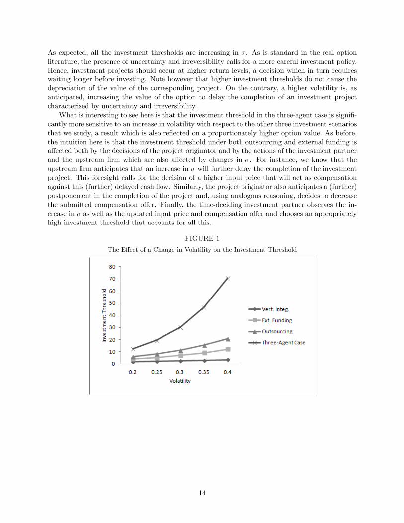
As expected, all the investment thresholds are increasing in �. As is standard in the real optionliterature, the presence of uncertainty and irreversibility calls for a more careful investment policy.Hence, investment projects should occur at higher return levels, a decision which in turn requireswaiting longer before investing. Note however that higher investment thresholds do not cause thedepreciation of the value of the corresponding project. On the contrary, a higher volatility is, asanticipated, increasing the value of the option to delay the completion of an investment projectcharacterized by uncertainty and irreversibility.

What is interesting to see here is that the investment threshold in the three-agent case is signi�-cantly more sensitive to an increase in volatility with respect to the other three investment scenariosthat we study, a result which is also re�ected on a proportionately higher option value. As before,the intuition here is that the investment threshold under both outsourcing and external funding isa¤ected both by the decisions of the project originator and by the actions of the investment partnerand the upstream �rm which are also a¤ected by changes in �. For instance, we know that theupstream �rm anticipates that an increase in � will further delay the completion of the investmentproject. This foresight calls for the decision of a higher input price that will act as compensationagainst this (further) delayed cash �ow. Similarly, the project originator also anticipates a (further)postponement in the completion of the project and, using analogous reasoning, decides to decreasethe submitted compensation o¤er. Finally, the time-deciding investment partner observes the in-crease in � as well as the updated input price and compensation o¤er and chooses an appropriatelyhigh investment threshold that accounts for all this.

FIGURE 1

The E¤ect of a Change in Volatility on the Investment Threshold

14

FIGURE 2

The E¤ect of a Change in Volatility on the Option Value

TABLE 4

The E¤ect of a Change in the Exogenous Cost Share on Timing and Option Value

� = 0 � = 0:1

Ext. Funding Three-Agent Case Ext. Funding Three-Agent Casey� 1.90 6.02 2.31 7.33FA 20.35 11.96 18.60 10.92FB 0 0 1.53 0.90FC - 3.77 - 2.83F 20.35 15.73 20.13 14.65

� = 0:5 � = 0:9

Ext. Funding Three-Agent Case Ext. Funding Three-Agent Casey� 3.97 12.56 5.61 17.79FA 14.50 8.52 12.35 7.26FB 3.48 2.04 3.77 2.21FC - 1.29 - 0.78F 17.98 11.85 16.12 10.25

In Table 4 we focus on the impact that a change in the exogenous investment cost share � mayhave. The benchmark value that we choose is � = 0:5 which implies a perfectly balanced investmentscheme with both partners undertaking equal portions of the sunk cost. We subsequently allow bothfor high (� = 0:9) and for low (� = 0:1) investment cost shares and we also present, for comparison�ssake, the case where there is no partnership (� = 0). Starting with the investment thresholds, wenote that a higher involvement of an investment partner always implies the postponement of theproject. Of course, keeping in mind the analysis of Section 3.4 and Section 4.1, this is hardly asurprise. As we have already seen there, a higher cost share � implies a higher nominal, but lowerreal, compensation o¤er from the project originator to the investment partner. Eventually, this isre�ected on a higher investment threshold and the further procrastination of the investment.

15

The e¤ect of a change in � on the option values of the three parties is nothing but an extensionof the e¤ect that we observe in the investment triggers. A higher � causes the depreciation of thevalue of the option to invest for every party apart from the investment partner who is favored bysuch a change. This adverse e¤ect is also clearly re�ected on the option value of the industry as awhole.

Lastly, in Table 5 we study the e¤ect of a change in the interest rate r. We start with thevertically integrated case. As far as the investment threshold is concerned, two opposing forces areacting. On one hand, an increase in r makes the potential investor more impatient since, with ahigher interest rate, the present becomes relatively more important than the future which impliesthe selection of a lower investment threshold. At the same time however, the increase in r impliesa decrease in the present value of the pro�t �ow that the project is meant to generate once it takesplace. This limits the interest of the potential investor to invest right now in a project which doesnot cover the high opportunity cost of capital. As we see in Table 5, the second force prevailscausing the postponement of the investment.

In the case where we deal with an investment partnership, an increase in the interest rate from0.05 to 0.06 causes a similar e¤ect but of smaller magnitude. The analysis of the previous paragraphholds here as well. However, we need to take into account the fact that the investment trigger isnow also a¤ected by the change in the compensation o¤er that is submitted to the time-decidingagent. The project originator, being impatient her/himself, is willing to make a more generouscompensation o¤er in an attempt to shorten the waiting period till the completion of the project.As one can see, this makes a di¤erence almost neutralizing the increase in r.

The most interesting cases involve the participation of the upstream �rm. Despite the fact thatthe argumentation from above still applies, the presence of an impatient upstream �rm causes, asone can see in Table 5, the acceleration of the investment. In order to understand the intuitionbehind this result, one should keep in mind that the e¤ect of a change in r is di¤erent for theupstream �rm than it is for the two investment partners. It is true that all the involved �rmsdiscount the value of the option to invest with a common discount factor.16 However, the way thateach agent evaluates the net present value of the project at the delivery date is di¤erent. For thetwo investment partners, the completion of the investment project signals the commencing of apro�t �ow that needs to be appropriately discounted. Of course, a change in r a¤ects the chosendiscounting factor. On the contrary, when the delivery date is reached, the upstream �rm receives alump sum which corresponds to the price of the input that s/he supplied and which is not a¤ectedby changes in r. As a consequence, even a small increase in the discount rate is enough to make theupstream supplier su¢ ciently impatient and willing to ask a lower input price as soon as this willlead to the acceleration of the investment. Indeed, in Table 5 we see that, when an upstream �rm ispresent, an increased discount rate encourages the acceleration of the completion of the project, aresult which is most prevalent in the three-agent case where the impatience of the two alien agentsconcurs.

As for the value of the option to invest, we see that even a slightly increased interest rate canconsiderably reduce the project�s option value. As we have already stressed above, an increasedinterest rate implies that the present becomes �nancially more important than the future. Hence,

16Recall that in Section 3.3 we have�

yyOS(pOS)

��both for A and for C, in Section 3.4 we have

�y

yV C( V C)

��both

for A and for B and in Section 4.1 we have�

yy3( 3;p3)

��for all three agents.

16

the option to delay an investment project for some future time point naturally becomes less valuable.

TABLE 5

The E¤ect of a Change in the Interest Rate on Timing and Option Value

r = 0:06

Vert. Integ. Ext. Funding Outsourcing Three-Agent Casey�=y�T1 1.16 1.02 0.97 0.84FA=F

T1A 0.54 0.52 0.50 0.49

FB=FT1B - 0.60 - 0.56

FC=FT1C - - 0.60 0.68

F=F T1 0.54 0.54 0.53 0.52

5 The compensation as the product of Nash bargaining

In Section 3.4 and in Section 4 we used a non-cooperative setting in order to describe the interactionbetween the potential investor A and the investment partner B. However, as noticed by the extantliterature, co-development partnerships are an increasingly utilized way of improving pro�tability,competitiveness and innovation e¤ectiveness.17 In the following, we will attempt to re-approachthe potential investor�s business plan using a cooperative framework. More precisely, we assumethat the compensation o¤er will now be replaced by a Nash bargaining solution that will explicitlyre�ect the bargaining power of the involved agents. We begin with the two-agent case and wesubsequently allow for outsourcing.

5.1 The input is produced in-house and the investment is partly externallyfunded

Similarly to the presentation of Section 3.4, we assume that A can produce the input in-house andthat the completion of the project is conditional on the participation of a �rm B who acts likean investment partner. As before, B is willing to undertake a share � of the sunk investment costgiven that s/he will receive compensation in return. What is new here with respect to the analysisof Section 3.4 is that, by assumption, A agrees with B on the compensation share and then decidesthe optimal investment threshold. Note that, contrary to the initial analysis, we now assume thatA, not B, is the time deciding agent. Apparently, A sacri�ces her/his exclusivity on the decisionof in order to become the time-deciding agent and similarly B sacri�ces her/his position as thetime-deciding agent in order to have a say in the decision of .18 In the following we see underwhat conditions this cooperative framework can replace the non-cooperative one.

Starting with the maximization problem of the time-deciding agent we have:

FAN (y) = maxyN ( )

�(1� ) yN ( )�M

r � a � (1� �) I��

y

yN ( )

��: (25)

Solving we obtain

yN ( ) =1� �1� y

V I : (26)

17See Zhou and Yang (2008), Biehl et al. (2006) and Cvitanic et al. (2011) respectively.18 In Appendix A we show how the analysis presented in Section 3.4 and Section 4 changes if A and B swap places.

In Appendix B we do the same for the analysis presented in Section 5 where the initial non-cooperative game-theoreticframework is replaced by a Nash bargaining solution and we show that such a change does not a¤ect the nature ofour main results.

17

Moving one step back, the two parties bargain anticipating that A will invest as soon as yt reachesthe trigger yN ( ). Given this, the new optimal compensation share is derived as the solution of

max N

� N

yN ( N )�Mr�a � �I

��B�(1� N )

yN ( N )�Mr�a � (1� �) I

��B�1�

y

yN ( N )

��, (27)

where �B represents B�s bargaining power.19 Solving we obtain

N =� (� � 1) + �B (1� �)

� � � : (28)

Combining Eq. (26) and Eq. (28) we have

yN ( N ) =� � �� � �B

yV I : (29)

One can check that the compensation N increases linearly in �B.20 It is also true that, contrary

to the compensation o¤ers that we have encountered in the previous sections, N is not alwaysincreasing in �, hence decreasing in volatility. More precisely, here we have @ N

@� ? 0 for � ? �B.In words, the compensation o¤er is decreasing in volatility only when the bargaining power of B issu¢ ciently low. Another interesting point is that when B bears almost the whole investment cost(� ! 1), we obtain N ' 1. Contrary to the compensation o¤er V C that cannot be larger than��1� , N can reach values as high as 100%, irrespective of the magnitude of �, if the cost share ofthe time-deciding agent A is small enough.

As far as the investment threshold is concerned, one can see that, as expected, yN ( N ) isincreasing in �B

21 and that in the special case where �B = � we have exactly yN ( N ) = yV I .In general, when the bargaining power of B is smaller (larger) than the exogenously given �, the

investment takes place ine¢ ciently early (late). Finally, one can check that@yN ( N )yV I

@� ? 0 for � ? �Bwhich means that when the bargaining power of B is su¢ ciently low (high), an increase in volatilityresults in a lower (higher) investment threshold yN ( N ) relative to y

V I .Given yN ( N ) and N , we can compute the value of the option to invest both for the potential

investor and for the investment partner. For A we obtain

FAN (y) = (1� �)�� � �B� � �

��F V IA (y), (30)

and for B we have

FBN (y) = �B

�� � �B� � �

���1F V IA (y):22 (31)

Of course the two agents will choose the Nash bargaining solution over the non-cooperative one only

if FAN (y) � F V CA (y) and FBN (y) � F V CB (y) or, alternatively, if (1� �)����B���

����

��1��1+�

���1and �B

����B���

���1� �

���1��1+�

��hold simultaneously.

19 It is assumed that the distribution of bargaining power is exogenous and that �A + �B = 1 with �A � 0 and�B � 0, where �i is the bargaining power of agent i with i 2 fA;Bg.20One can also check that N is increasing and convex in �.21One can also check that yN ( N ) is linearly decreasing in �.22Note that, as expected, @FiN (yt)

@�i> 0; i 2 fA;Bg.

18

It is interesting to see that the condition FAN (y) � F V CA (y) implies � > �B which basicallymeans that the Nash bargaining solution guarantees that the investment will take place (ine¢ -ciently) early: yN ( N ) < yV I . Let�s recall that when we solved the same problem under thenon-cooperative framework in Section 3.4, we found that the investment would take place inef-�ciently late: yV C( V C) > yV I . Comparing these two results we derive a quite straightforwardconclusion: the adopted game-theoretic framework determines the nature of the interaction be-tween A and B as well as the way that this is re�ected on the chosen investment threshold andthe value of the option to invest. The importance of this statement will become clearer in the nextsection where the three-agent case is discussed. Summing up our results:

Proposition 9 In the case where the input is produced in-house and the completion of the projectdepends on external funding, the Nash bargaining solution can replace the non-cooperative one when

the participation conditions FAN (y) � F V CA (y) ) (1� �)����B���

����

��1��1+�

���1and FBN (y) �

F V CB (y) ) �B

����B���

���1� �

���1��1+�

��are satis�ed. If this is the case, then the investment

occurs when the scale parameter reaches a threshold yN ( N ) =������B

yV I . Notably, FAN (y) �F V CA (y)) � > �B ) yN ( N ) < yV I which means that a Nash bargaining solution guarantees thatthe investment will take place ine¢ ciently early.

For instance, for � = 0:025; � = 0:2; r = 0:05; y0 = �M = 1; � = 0:5 and I = 24, the Nashbargaining solution can take place for any �B 2 [0:147; 0:236]. If e.g. �B = 20%, we have yN =1:45; FAN = 15:13 and FBN = 4; 61. Comparing these with the corresponding values of Table 1 wesee that, as expected, the option values of both parties are appreciated and that the investmentthreshold under Nash bargaining is smaller than the investment threshold under vertical integration.

5.2 The three-agent case

Let�s now see what is di¤erent if a third agent is involved in the completion of the project. Similarlyto the presentation of Section 4 it is assumed that the input is produced by an external supplierwith market power. The game evolves in the following way:

1. The upstream �rm C decides the input price that maximizes her/his individual option value.2. Given the price of the input, A and B engage in a Nash bargaining in order to decide the

compensation that A will submit to B and �nally,3. A decides what is the optimal investment threshold given the price of the input and the

decided compensation.Moving backwards, we begin by studying the behavior of A. The optimal investment threshold

in the three-agent case is derived as the solution of the following maximization problem:

FA3N (y) = maxy3N ( ;p)

�(1� ) y3N ( ; p)�M

r � a � (1� �) p��

y

y3N ( ; p)

��(32)

From the �rst-order condition we obtain

y3N ( ; p) =�

� � 1r � a�M

p1� �1� : (33)

Given y3N ( ; p), A and B engage in a Nash bargaining in order to commonly decide the optimalcompensation 3N which is derived as the solution of

max 3N

� 3N

y3N ( 3N )�Mr�a � �I

��B�(1� 3N )

y3N ( 3N )�Mr�a � (1� �) I

��B�1�

y

y3N ( 3N )

��: (34)

19

Solving we obtain

3N =� (� � 1) + �B (1� �)

� � � : (35)

Unsurprisingly, we �nd 3N = N : The intuition behind this result is that, as in the non-cooperativecase, the presence/absence of C does not a¤ect the interaction between A and B since the exoge-nously given cost share � has to do with the generic investment cost no matter if that is I orp.

Finally, the input supplier C observes how A and B behave and chooses the familiar p3N =���1I

solving FC3N (y) = maxp3N

(p3N � I)�

yy3N ( 3N ;p3N )

��. Apparently, the price that maximizes the value

of the option to invest for the upstream �rm is not a¤ected by the distribution of bargaining powerbetween A and B. Again, C is indi¤erent to the means that A uses to fund her/his project.

Now, substituting 3N and p3N in the formula for the investment threshold we obtain

y3N ( 3N ; p3N ) =�

� � 1� � �� � �B

yV I > yN ( N ) : (36)

Similarly to yN ( N ), the threshold y3N ( 3N ; p3N ) is increasing in �B.23 One can also check that,

contrary to the two-agent case where we had@yN ( N )yV I

@� ? 0 for � ? �B, here we have@y3N ( 3N;p3N )

yV I

@� < 0which means that as the volatility of the scale parameter increases, the relative investment thresholdgets larger, irrespective of how �B compares to �. This has to do with the fact that the deliveryprice p3N , contrary to I, is increasing in the volatility of the scale parameter and, as a result, thereis no level of bargaining power low enough to guarantee a negative relationship between the relativeinvestment threshold and the volatility. As a consequence, we have y3N ( 3N ; p3N ) > yV I . Notethat this is the result of two opposing forces. On one hand, the interaction between A and B drivesthe investment threshold below yV I but,24 on the other, the e¤ect of the presence of C has theopposite direction.25 Apparently the second one prevails. It is interesting to recall here that whenwe discussed the three-agent case under the non-cooperative setting in Section 4, we similarly hady3 ( 3; p3) > yV I . However, there the two e¤ects were not opposing but, on the contrary, they werecomplementing each other. As a result, the importance of explicitly taking C into account was, tosome extent, less obvious.

We conclude with the value of the option to invest for the three agents and we have

FA3N (y) = (1� �)�� � 1�

���1�� � �B� � �

��F V IA (y); (37.1)

FB3N (y) = �B

�� � 1�

���1�� � �B� � �

���1F V IA (y); (37.2)

FC3N (y) =

�� � 1�

�� �� � �B� � �

��F V IA (y): (37.3)

A andB will choose the Nash bargaining solution over the non-cooperative one only if FA3N (y) �FA3(y) and FB3N (y) � FB3(y). As in the previous section, we �nd that if the conditions (1� �)

����B���

����

��1��1+�

���1and �B

����B���

���1� �

���1��1+�

��hold simultaneously, then both A and B are better

23Note that, similarly to yN ( N ), y3N ( 3N ; p3N ) is linearly decreasing in �.24This �rst e¤ect was discussed in Section 5.1.25This second e¤ect was discussed in Section 3.3.

20

o¤. Once again this has to do with the fact that the presence/absence of C does not a¤ect theinteraction between A and B. Finally, as far as C is concerned, the Nash bargaining solution is

preferred to the non-cooperative one when FC3N (y) � FC3(y) )����B���

��>�

��1��1+�

��. One

can easily check that this is always the case since FA3N (y) � FA3(y) implies FC3N (y) � FC3(y).Concluding we have:

Proposition 10 In the case where the input is outsourced and the completion of the project de-pends on external funding, the Nash bargaining solution can replace the non-cooperative one whenthe participation conditions FA3N (y) � FA3(y) , FAN (y) � F V CA (y) and FB3N (y) � FB3(y) ,FBN (y) � F V CB (y) hold simultaneously. If this is the case, the investment occurs when the scaleparameter reaches a threshold y3N ( 3N ; p3N ) =

���1

������B

yV I > yV I i.e. the investment takes place

ine¢ ciently late. Despite the fact that the presence of B favors the acceleration of the project26 thepresence of C, which dictates the postponement of the investment, prevails.

For instance, for � = 0:025; � = 0:2; r = 0:05; y0 = �M = 1; � = 0:5 and I = 24, the Nashbargaining solution can take place, as before, for any �B 2 [0:147; 0:236]. If e.g. �B = 20%, wehave: y3N = 4:59; FA3N = 8:89, FB3N = 2; 71 and FC3N = 5; 61. Comparing these with thecorresponding values of Table 1 we see that, as expected, the option values of all three parties areappreciated and that the investment threshold under Nash bargaining is larger than the investmentthreshold under vertical integration.

6 Epilogue

In this paper we consider the investment problem of a �rm who contemplates entering an uncertainnew market under two conditions. On one hand, an upstream �rm with market power is responsiblefor the provision of a discrete input that is a prerequisite for the completion of the project and, onthe other, an exogenously given share of the sunk investment cost is undertaken by an investmentpartner who claims a share of the project as compensation in return.

Following the real option approach, we build a stochastic dynamic programming model in orderto study the interaction among these three agents and we �nd the following. Firstly, we verifythat the optimal investment timing and, consequently, the maximum value of the option to investare reached when the potential investor acts autonomously (vertically integrated case). On thecontrary, the presence of any additional agent involved in the completion of the project causes thedelay of the investment which, as we show, also implies a smaller value of the option to invest.However, despite the fact that the presence of any additional agent a¤ects the timing and the valueof the option to invest the same way, the magnitude of the e¤ect itself is not the same. Actually,a comparison between external funding and input outsourcing denotes that the former is alwayspreferred to the latter.

Secondly, we focus on the three-agent case and we �nd that the synchronous involvement ofan upstream supplier and an investment partner in the project, constitutes the worst-case scenariosince we basically deal with a combination of the corresponding distorting e¤ects. In this case,the value of the option to invest reaches its minimum whereas the investment threshold reaches itsmaximum.

In the last part of the paper we present the conditions under which it is possible to replacethe original non-cooperative setting with a Nash bargaining solution and we show that, even in

26See Proposition 9.

21

that case, the optimal investment threshold is unattainable. Actually, our analysis shows that ifthe upstream �rm is absent (i.e. the input is produced in-house) the project realizes ine¢ cientlyearly whereas, if the upstream �rm is present (i.e. the input is outsourced) it realizes ine¢ cientlylate. This is, again, evidence of the importance of the nature of the sunk investment cost whenmodelling investment projects characterized by uncertainty and irreversibility, especially if insteadof a single potential investor, an investment partner is also involved in their completion.

22

A Appendix

A.1 The input is produced in-house and the investment is partly externallyfunded: A review of Section 3.4

In the main body of the paper we describe the interaction between a potential investor A and aninvestment partner B following the presentation by Lukas and Welling (2014) according to whichA is the game-leader submitting the compensation o¤er and B is the game-follower choosing theinvestment timing. This framework seems suitable to describe the e¤orts of a potential investor whoseeks out funding for the business plan that is under consideration. However, one can also considerthe case where B is the game-leader submitting the compensation o¤er and A is the game-followerdeciding the investment timing. This framework seems more appropriate to describe partnershipsin which a venture capitalist makes the �rst step declaring her/his interest to invest in an emerging�rm.27

Moving backwards, we �nd that the solution of A�s decision problem gives an investment thresh-old yRV C = 1��

1� yV I whereas the solution of B�s decision problem gives a compensation share

RV C = 1�2�+����� .28 Combining the two we �nd that the optimal investment threshold is given by

yRV C� RV C

�=� � �� � 1y

V I�> yV I

�: (A.1)

As far as the value of the option to invest is concerned, we �nd that for the potential investor Awe have

FRV CA (y) = (1� �)�� � 1� � �

��F V IA (y), (A.2)

whereas for the investment partner B we obtain

FRV CB (y) =

�� � 1� � �

���1F V IA (y): (A.3)

One can easily check that, similarly to what we �nd in Section 3.4, the presence of �rm Bcauses the postponement of the project29, making the potential investor worse o¤ with respect tothe vertically integrated case.

A.2 The three-agent case: A review of Section 4

In this section we review the three-agent case as presented in Section 4 assuming however that Aand B swap places. More precisely:

1. C is still the game-leader who decides the input price.2. Given the price of the input, B decides what is the optimal compensation that s/he should

ask from A and3. A decides what is the optimal investment threshold given the price of the input and the

compensation share.Solving backwards, from the potential investor�s maximization problem we obtain y3R ( ; p) =

���1

1��1�

r�a�M

p. Taking this into consideration, the investment partner is choosing 3R =1�2�+�����

27Cvitanic et al. (2011) present a similar case.28Check that RV C , similarly to V C , is increasing in �, but contrary to V C is decreasing in �.29Note that yRV C , similarly to yV C , is decreasing in �, but contrary to yV C is decreasing in �.

23

�= RV C

�.30 Finally, the upstream �rm, keeping in mind the reactions of A and B, decides the

optimal price of the input p3R =���1I. Plugging the compensation o¤er and the input price in the

formula for the investment threshold we obtain

y3R ( 3R; p3R) =�

� � 1� � �� � 1y

V I�> yV I

�: (A.4)

Given this, we also have

FA3R(y) = (1� �)�� � 1�

���1�� � 1� � �

��F V IA (y); (A.5.1)

FB3R(y) =

�� � 1�

���1�� � 1� � �

���1F V IA (y); (A.5.2)

FC3R(y) =

�� � 1�

�� �� � 1� � �

��F V IA (y): (A.5.3)

Similarly to Section 4, we �nd that the synchronous presence of B and C causes the postponementof the project and that this is also re�ected on A�s option value.

Finally, note that from Eq. (A.2), Eq. (A.3) and Eq. (A.5) we �nd that FRV C(y) =2�����1��1

���1���

��F V IA (y) and F3R(y) =

�1� � + ���

��1 +��1�

����1�

���1 ���1���

��F V IA (y).31 Sum-

ming up

Proposition 11 A comparison among the option values and the investment triggers derived inSection A.1 and Section A.2 of Appendix A gives the following rankings:

1) y3R ( 3R; p3R) > yOS�pOS

�> yRV C

� RV C

�> yV I ,

2) F3R(y) < FOS(y) < FRV C(y) < F V IA (y),3) FA3R(y) < FRV CA (y) < FOSA (y) < F V IA (y),4) FB3R(y) < FRV CB (y) and5) FC3R(y) < FOSC (y).

Comparing Proposition 11 (where B is the game-leader and A is the game-follower) with Propo-sition 8 (where A is the game-leader and B is the game-follower) we �nd that, in both cases, asthe number of agents involved in an investment project increases, the completion of the project ispostponed at the expense of the project�s option value both in the �rm and in the industry level.We also �nd that the rankings of the investment thresholds and the aggregate option values remainthe same whereas the only di¤erence that we observe has to do with the ranking of A�s optionvalues. As one can see, when A is the game-follower (game-leader), an interaction with C (B) ispreferred to an interaction with B (C) which means that the way that A is a¤ected by the presenceof the alien �rms depends on the role that s/he has in the game.

Another interesting point is that FRV CA (y) < F V CA (y) and FRV CB (y) > F V CB (y) which meansthat being the game-leader is always preferable, no matter the values of � and �. Finally, onecan also check that yRV C

� RV C

�? yV C

� V C

�and y3R ( 3R; p3R) ? y3 ( 3; p3), and consequently

that FRV C(y) 7 F V C(y) and F3R(y) 7 F3(y), when 0:5 ? �. In words, it is socially optimal forthe agent who undertakes the lion�s share of the sunk investment cost to be the game-leader eitherwhen the input is outsourced or not. This means that the analysis of the main body of the paperwhere A is the game-leader and B is the game-follower would be preferred from a social point ofview for 0:5 < � whereas the analysis presented here would be socially preferable for 0:5 > �.30Check that the equality 3R = RV C is analogous to the equality 3 = V C that we �nd in Section 4 of the

main body of the paper.31We de�ne FRV C(y) � FRV CA (y) + FRV CB (y) and F3R(y) � FA3R(y) + FB3R(y) + FC3R(y).

24

B The compensation as the product of Nash bargaining

B.1 The input is produced in-house and the investment is partly externallyfunded: A review of Section 5.1

In Section A.1 of Appendix A we presented a leader-follower game where B decides the compensa-tion and, given that, A chooses the optimal investment threshold. Let�s now see what is di¤erentif the compensation is the product of bargaining between the two agents. The game evolves in thefollowing way: initially A and B bargain over the compensation share and then, given that, Bdecides the optimal investment threshold. Notice that contrary to Section A.1, the time-decidingagent is B, not A. Alternatively put, our goal in this section is to �nd the conditions under whichA would be willing to let B decide the timing of the investment, given that the compensation sharewill be the product of bargaining between the two agents instead of a unilateral decision of B.

Starting with the maximization problem of the time-deciding agent B we obtain yNR =� y

V I .Moving one step back, the two parties bargain anticipating that B will invest as soon as yt reachesthe threshold yNR. Given this, the bargaining over the compensation share gives NR = � ��1+�B��1+�32and, consequently,

yNR( NR) =� � 1 + �� � 1 + �B

yV I .33 (B.1)

Given the compensation o¤er and the optimal investment threshold, we can compute the valueof the option to invest both for the potential investor and for the time-deciding investment partner.More precisely, for A we obtain

FANR(y) = (1� �B)�� � 1 + �B� � 1 + �

���1F V IA (y), (B.2)

and for B we have

FBNR(y) = �

�� � 1 + �B� � 1 + �

��F V IA (y): (B.3)

As expected, A and B will choose the Nash bargaining solution over the non-cooperative one

only if FANR(y) � FRV CA (y) and FBNR(y) � FRV CB (y) or, alternatively, if (1� �B)���1+�B��1+�

���1�

(1� �)���1���

��and �

���1+�B��1+�

������1���

���1hold simultaneously. One can also easily check that

the condition FBNR(y) � FRV CB (y) implies � < �B which means that any Nash bargaining solutionguarantees that the investment will take place (ine¢ ciently) early. Note that this is no di¤erentfrom what we found in Section 5.1 of the main body of the paper.

B.2 The three-agent case: A review of Section 5.2

Let�s now see what is di¤erent if the input is outsourced. Our starting point is again the investmentthreshold decision by B. From the �rst-order condition we have y3NR( ; p) =

���1

r�a�M

p � . Movingone step back, A and B bargain anticipating that B will invest as soon as yt reaches the chosen

32One can check that the compensation share NR increases linearly in �B and that it is also increasing and concavein �. Finally, @ NR

@�? 0 for � ? �B .

33yNR( NR) is decreasing in �B , linearly increasing in � and, with respect to �, we have@yNR( NR)

yV I

@�? 0 if �B ? �.

This basically means that in the special case where �B = � we have exactly yNR( NR) = yV I but, in general, whenthe bargaining power of B is su¢ ciently low (high), an increase in volatility results in a higher (lower) investmentthreshold yNR( NR) relative to y

V I .

25

threshold and eventually choose 3NR = � ��1+�B��1+� (= NR).34 Finally, the game-leader C observes

the behavior of A and B and decides the input price p3NR =���1I.

Substituting the optimal price and the compensation o¤er in the investment threshold fromabove we have

y3NR( 3NR; p3NR) =�

� � 1� � 1 + �� � 1 + �B

yV I : (B.4)

Note that y3NR( 3NR; p3NR) > yV I .35 This is the result of two opposing forces. On one hand,the interaction between A and B drives the investment trigger below yV I but,36 on the other, thee¤ect of the presence of C has the opposite direction.37 Apparently, the second one prevails. Itis interesting to recall that Eq. (A.4) that corresponds to the non-cooperative case gives also aninvestment threshold higher than yV I : y3R ( 3R; p3R) > yV I . However, there the two e¤ects werenot opposing but, on the contrary, they were complementing each other. Note that our analysishere is totally symmetric to the one presented in Section 5.2 of the main body of the paper.

Keeping in mind the formulas for 3NR, p3NR and y3NR( 3NR; p3NR), the option values for thethree agents are

FA3NR(y) = (1� �B)�� � 1�

� � 1 + �B� � 1 + �

���1F V IA (y); (B.5.1)

FB3NR(y) = �

�� � 1�

���1�� � 1 + �B� � 1 + �

��F V IA (y); (B.5.2)

FC3NR(y) =

�� � 1�

�� �� � 1 + �B� � 1 + �

��F V IA (y): (B.5.3)

A andB will choose the Nash bargaining solution over the non-cooperative one only if FA3NR(y) �FA3R(y) and FB3NR(y) � FB3R(y) or, alternatively, if the familiar (1� �B)

���1+�B��1+�

���1�

(1� �)���1���

��and �

���1+�B��1+�

������1���

���1hold simultaneously. As far as C is concerned,

the Nash bargaining solution is preferred to the non-cooperative one when FC3NR(y) � FC3R(y))���1+�B��1+�

������1���

��. One can easily see that this is always the case since FB3NR(y) � FB3R(y)

implies FC3NR(y) � FC3R(y). Concluding we have:

Proposition 12 In the case where the input is outsourced and the completion of the project dependson external funding, the Nash bargaining solution38 can replace the non-cooperative one39 when theparticipation conditions FA3NR(y) � FA3R(y), FANR(y) � FRV CA (y) and FB3NR(y) � FB3R(y),FBNR(y) � FRV CB (y) hold simultaneously. If this is the case, the investment occurs when the scaleparameter reaches a threshold y3NR( 3NR; p3NR) =

���1

��1+���1+�B

yV I > yV I i.e. the investment takes

place ine¢ ciently late. Despite the fact that the presence of B favors the acceleration of the project40

the presence of C, which dictates the postponement of the investment, prevails.

34Check that the equality 3NR = NR is analogous to the equality 3N = N that we �nd in Section 5.2 of themain body of the paper.

35Note also that@y3NR( 3NR;p3NR)

yV I

@�< 0.

36This e¤ect was discussed in Section B.1 of Appendix B.37This e¤ect was discussed in Section 3.3 of the main body of the paper.38Section B.2 of Appendix B.39Section A.2 of Appendix A.40According to Section B.1 of Appendix B.

26

References

[1] Alvarez LHR, Stenbacka R. 2007. Partial outsourcing: a real options perspective. InternationalJournal of Industrial Organization 25: 91�102.

[2] Azevedo A, Paxson D. 2014 Developing real option game models, European Journal of Oper-ational Research 237: 909-920.

[3] Banerjee S, Güçbilmez IU, Pawlina G. 2014. Optimal exercise of jointly held real options:a Nash bargaining approach with value diversion. European Journal of Operational Research239 (2): 565-578.

[4] Benson D, Ziedonis RH. 2009. Corporate venture capital as a window on new technologies:Implications for corporate investors when acquiring startups. Organization Science 20: 352-376.

[5] Biehl M, Cook W, Johnston DA. 2006.The e¢ ciency of joint decision making in buyer-supplierrelationships. Annals of Operations Research 145:15-34.

[6] Billette de Villemeur E, Ruble R, Versaevel B. 2014. Investment timing and vertical relation-ships. International Journal of Industrial Organization 33: 110-123.

[7] Chen P. 2012. The investment strategies for a dynamic supply chain under stochastic demands.International Journal of Production Economics 139: 80-89.

[8] Chesbrough H, Schwartz K. 2007. Innovating business models with co-development partner-ships. Research Technology Management 50: 55-59.

[9] Chevalier-Roignant B, Flath CM, Huchzermeier A, Trigeorgis L. 2011. Strategic investmentunder uncertainty: a synthesis. European Journal of Operational Research 215: 639-650.

[10] Cvitanic J, Radas S, �ikic H. 2011. Co-development ventures: optimal time of entry andpro�t-sharing. Journal of Economic Dynamics and Control 35(10): 1710-1730.

[11] Di Corato L, Moretto M, Rossini G. 2017. Financing �exibility: The case of outsourcing.Journal of Economic Dynamics and Control 76: 35-65.

[12] Dixit A. 1993, The art of smooth pasting, Fundamentals of Pure and Applied Economics 55,Routledge.

[13] Dixit A, Pindyck RS. 1994. Investment under Uncertainty. Princeton University Press, Prince-ton.

[14] Dushnitsky G, Lenox MJ. 2005a. When do incumbents learn from entrepreneurial ventures?Corporate venture capital and investing �rm innovation rates. Research Policy 34: 615-639.

[15] Dushnitsky G, Lenox MJ. 2005b. When do �rms undertake R&D by investing in new ventures?Strategic Management Journal 26(10): 947-965.

[16] Folta TB. 1998. Governance and uncertainty: The trade-o¤ between administrative controland commitment. Strategic Management Journal 19: 1007-1028.

[17] Folta TB, Miller KD. 2002. Real options in equity partnerships. Strategic Management Journal23: 77-88.

27

[18] Guimarães Dias M, Teixeira J. 2010. Continuous-Time Option Games: Review of Models andExtensions. Multinational Finance Journal 14: 219-254.

[19] Huisman K, Kort PM, Pawlina G, Thijssen J. 2004. Strategic investment under uncertainty:Merging real options with game theory. Zeitschrift fr Betriebswirtschaft 74: 97-123.

[20] Kogut B. 1991. Joint ventures and the option to expand and acquire. Management Science37: 19-33.

[21] Kogut B, Kulatilaka N. 1994. Operating �exibility, global manufacturing, and the option valueof a multinational network. Management Science 40: 123-139.

[22] Lambrecht BM. 2004. The timing and terms of mergers motivated by economies of scale.Journal of Financial Economics 72(1): 41-62.

[23] Li J, Dhanaraj C, Shockley RL. 2008. Joint venture evolution: extending the real optionsapproach. Managerial and Decision Economics 29: 317-336.

[24] Lukas E, Mölls S, Welling A. 2016. Venture capital, staged �nancing and optimal fundingpolicies under uncertainty. European Journal of Operational Research 250(1): 305-313.

[25] Lukas E, Welling A. 2014. Investment timing and eco(nomic)-e¢ ciency of climate-friendlyinvestments in supply chains. European Journal of Operational Research 233(2) (Special Issue:Eco-E¢ cient Green Supply Chain Management): 448-457.

[26] McDonald R, Siegel D. 1986. The value of waiting to invest. Quarterly Journal of Economics101(4): 707-728.

[27] McGrath RG. 1997. A real options logic for initiating technology positioning investments.Academy of Management Review 22: 974-996.

[28] McGrath RG, Nerkar A. 2004. Real options reasoning and a new look at the R&D investmentstrategies of pharmaceutical �rms. Strategic Management Journal 25: 1-21.

[29] Miller M, Modigliani F. 1961. Dividend policy, growth, and the valuation of shares. The Journalof Business 34(4): 411-433.

[30] Morellec E, Zhdanov A. 2005. The dynamics of mergers and acquisitions. Journal of FinancialEconomics 77(3): 649-672.

[31] Moretto M, Rossini G. 2012. Flexible outsourcing. Managerial and Decision Economics 33:47-59.

[32] Mulherin JH, Boone AL. 2000. Comparing acquisitions and divestures. Journal of CorporateFinance 6: 117-139.

[33] Myers SC. 1977. Determinants of corporate borrowing. Journal of Financial Economics 5(2):147-176.

[34] O�Brien JP, Folta TB, Johnson DR. 2003. A real options perspective on entrepreneurial entryin the face of uncertainty. Managerial and Decision Economics 24: 515-533.

[35] Puranam P, Singh H, Chaudhuri S. 2009. Integrating acquired capabilities: when structuralintegration is (un)necessary. Organization Science 20(2): 313-328.

28

[36] Quinn JB. 2000. Outsourcing innovation: the new engine of growth. Sloan Management Review41: 13-28.

[37] Reuer JJ, Tong TW. 2007. Corporate investments and growth options. Managerial and Deci-sion Economics 28: 863-877.

[38] Roberts EB, Berry CA. 1985. Entering new business: selecting strategies for success. SloanManagement Review 26(2): 57-71.

[39] Teixeira JCA. 2014. Outsourcing with debt �nancing. Portoguese Economic Journal 13: 1-24.

[40] Tirole J, 1988. The Theory of Industrial Organization. MIT Press, Cambridge.

[41] Tong TW, Li Y. 2011. Real options and investment mode: evidence from corporate venturecapital and acquisition. Organization Science 22(3): 659-674.

[42] Triantis A, Hodder J. 1990. Valuing �exibility as a complex option. The Journal of Finance45(2): 549-565.

[43] Vrande van de VJA, Vanhaverbeke W. 2013. How prior corporate venture capital investmentsshape technological alliances: a real options approach. Entrepreneurship Theory and Practice37 (5): 1019-1043.

[44] Zhou Y-W, Yang S. 2008. Pricing coordination in supply chains through revenue sharingcontracts. Information and Management Sciences 19 (1): 31-51.

29