Vers. 01 User’s guide & Tutorial

February 2012

K-NN FOREST © is Copyrighted by BioFor Italy and GM WEB STUDIO

2

This software is property of GM Web Studio and Biofor Italy S.r.l. (Spin Off of the University of Tuscia) Lead programmer: Alessandro Mastronardi Source code property of GM Web Studio by Alessandro Mastronardi Scientific responsible and project coordinator: Gherardo Chirici Scientific supervisors: Piermaria Corona and Marco Marchetti Scientific team: Davide Travaglini, Roberta Bertini, Nicola Puletti Developers of the first original source codes: Fabio Maselli and Lorenzo Bottai The project of the software k-NN Forest is developed also within the framework of the activities of forestlab.net consortium (www.forestlab.net) This software is provided free of charge for research purposes. We will be happy to receive your feedbacks, successful stories, problems or suggestions for future versioning of K-NN FOREST. Write to: gherardo.chirici@unimol.it Please cite this document as: Chirici, G., P. Corona , M. Marchetti, Mastronardi A., Maselli F., Bottai L., Travaglini D., 2012. K-NN FOREST. User’s guide and tutorial. Available on-line at www.forestlab.net. Please cite also this paper, it was the first one entirely developed with K-NN FOREST: Chirici, G., A. Barbati, P. Corona, M. Marchetti, D. Travaglini, F. Maselli, and R. Bertini. 2008. Non-parametric and parametric methods using satellite images for estimating growing stock volume in Alpine and Mediterranean forest ecosystems. Remote Sensing of Environment 112(5):2686-2700.

3

Contents 1. Introduction ...................................................................................................................................... 4  

1.1. k-Nearest Neighbors ....................................................................................................... 4  1.2 Multidimensional distance .............................................................................................. 5  1.3 Optimizing k-NN ................................................................................................................ 6  References ................................................................................................................................... 6  

2. Manual .......................................................................................................................................... 9  2.1 System requirements ...................................................................................................... 9  2.2 You need IDRISI! .............................................................................................................. 9  2.3 Getting started with k-NN Forest ................................................................................ 9  2.4 k-NN Forest display panel .............................................................................................. 9  2.5 How does k-NN Forest works? ................................................................................... 10  

2.5.1 Working dataset ...................................................................................................... 10  2.5.2 Set up .......................................................................................................................... 11  2.5.3 Extract ......................................................................................................................... 12  2.5.4 Optimization .............................................................................................................. 13  2.5.5 Estimation .................................................................................................................. 14  

3. Tutorial ....................................................................................................................................... 16  3.1 Setting up k-NN Forest ................................................................................................. 16  3.2 Extract multispectral features .................................................................................... 17  3.3 Choose the optimal k-NN configuration ................................................................. 20  3.4 k-NN estimation ............................................................................................................... 25  

4

1. Introduction This software is intended The k-Nearest Neighbors (k-NN) method is one of the most successful approaches for biophysical forest attributes estimation using field measurements and remote sensing data. The first tests were probably developed within the Finnish National Forest Inventory (Tomppo,1991). The theory of the k-NN method is described in several scientific papers. Here follow a non exhaustive introduction to the k-NN for those people who are not familiar with it. More detailed information on the k-NN method and its applications are provided by e.g. Tokola et al., 1996; Franco-Lopez et al., 2001; Katila and Tomppo, 2001; Holmström, 2002; Katila and Tomppo 2002; McRoberts et al., 2002; Tomppo et al., 2002; Tuominen et al., 2003; Tomppo and Halme, 2004; Gjertsen, 2005; McInerney et al., 2005; Koukal et al., 2005; Nilsson et al., 2005; Tomppo, 2005; Baffetta et al., 2007; Chirici et al. 2008; Finley et al., 2008; McRoberts, 2008.; McRoberts, 2009; Baffetta et al., 2011; McRoberts et al., 2011. Two workshops were organized on k-nn applications in forestry: the first one was hosted by the University of Minnsesota (USA) in July 2006, the second one was hosted by the Italian Academy of Forest Sciences (Florence, Italy) in July 2007. You may access the workshops websites and the on-line proceedings at: http://knn.gis.umn.edu/ 1.1. k-Nearest Neighbors The k-NN is a non-parametric method used to estimate the dependent variable Y (e.g. basal area, forest growing stock volume, biomass) for a population composed by N elements. The k-NN method assumes that the true values of auxiliary variables (independent variables) related to Y are knew for all of the N elements of the population whereas the true value of Y is knew just for a sample of n elements. Usually the population is represented by pixel of remotely sensed image. The dependent variable Y is measured on field survey units in correspondence of the n pixel of the sample, here in after named the reference set, whereas the values of the auxiliary variables represented by digital number (DN) of multispectral satellite bands as well as by indices computed by satellite imagery and other independent variables correlated to Y (e.g. elevation, aspect, slope, site fertility etc.) are knew for all of the N pixel of the population. The unknown value of the dependent variable Y for each t-th pixel of the set N-n, here in after named the target set, can be estimated as weighted mean of the Y values measured in k units of the reference set nearest to the t-th pixel in the multidimensional space defined by the auxiliary variables:

∑

∑

=

== k

iti

k

iiti

t

W

YWY

1,

1,

ˆ [1]

5

where the weight W can be set equal to 1/k (in this case tY is equal to the arithmetic mean of the Y values measured in the k pixel of the reference set nearest to the t-th pixel) or it is computed as inversely proportional to the multidimensional distance between the t-th pixel and each of the k nearest pixel of the reference set. 1.2 Multidimensional distance The multidimensional distance is measured in the feature space defined by auxiliary variables. The multidimensional distance can be computed by means of several measures. In k-NN Forest software three different distance measures are available: the Euclidean Distance, the Mahalanobis Distance, the Distance weighted with Fuzzy weights or Fuzzy Distance (Chirici et al., 2008). The Euclidean Distance (ED), which is equivalent to the geometric distance measured in the multidimensional feature space, is the simplest and most used distance measure (De Maesschalck et al., 2000). ED between reference and target pixels can be computed as:

∑=

−=n

1iii )XtXr(ED [2]

where n is the number of feature space variables and Xri and Xti are the values of the reference and sample pixels in feature space variable i, respectively. ED considers all feature space variables without taking into account their multicollinearity. The Mahalanobis Distance (MD) introduces a correction for this factor by considering the variance–covariance matrix of the feature space variables, C (Richards, 1993). MD between reference and target pixels is computed as:

( ) ( )XtXrC'XtXrMD 1 −−= − [3] where Xr and Xt are the n-dimensional feature space vectors of the reference and target pixels, respectively, and C can be derived from the reference data set. As can be easily understood, neither ED or MD emphasizes the relationship of the feature space variables to the response variable. In order to overcome this limitation, modified forms of multidimensional distances have been proposed aiming at giving preferential consideration to the most informative feature space variables (Holmström et al., 2001; Maselli et al.,2005). The Distance weighted with Fuzzy weights or Fuzzy Distance (FD) is a modification of MD where the variance–covariance matrix is computed in a fuzzy way. The fuzzy variance–covariance C* is obtained by weighting the reference pixels through fuzzy membership grades that give preferential consideration to reference pixels with values of the response variable close to

6

the mean (Maselli, 2001). This is obtained deriving the membership grade of each reference pixel j, Fgj, from the Gaussian probability density function of the response variable, through (Anderson, 1984):

( ) ( ) 22j /Y2/112/1

i e2Fg σµσπ −−−−= [4] where: Yj = value of the response variable at reference pixel j; µ = mean value of the response variable; σ2 = variance of the response variable. This modification results in a reduction of the variance–covariances of the feature space variables most correlated with the response variable and therefore most informative on it. Consequently these variables become the most important in the calculation of FD between reference and target pixels:

( ) ( )XtXrC'XtXrFD 1 −−= −∗ [5] 1.3 Optimizing k-NN Accuracy of k-NN estimates are influenced by several factors such as the type and number of feature space variables, multidimensional distance measures and number of k nearest neighbors. One way to empirically optimize the k-NN configuration is to test all the possible configuration. But the k-NN method is computing intensively and this approach carried out for all the pixels of the target set would be very tedious. For this reason it is possible to decide the local “best” k-NN configuration calculating the k-NN estimates for all the possible configurations in the reference pixels ONLY. Speeding up a lot the computing time. This method is a bootstrapping technique called Leave-One-Out (LOO) cross-validation technique (Lachenbruch & Mickey, 1986). The performance for each k-NN configuration tested with LOO may be assessed calculating the correlation between k-NN estimates and measures of the response variable or calculating an indicator of the k-NN error estimates such as the Root Mean Square Error (RMSE) (Franco-Lopez et al., 2001). The best k-NN configuration, that one with the minimum error in the estimates and the maximum correlation between estimates and measured values of the response variable, will be used to perform the final k-NN estimation of the dependent variable Y for all the pixels of the target set. References Anderson, T.W. (1984). An introduction to multivariate statistical analysis. New

York: John Wiley & Sons. Baffetta, F., Chirici, G., Corona, P., Fattorini, L., & Franceschi, S. (2007). A

design-based approach to k-NN technique in forest inventories. In, Forestsat 2007. Montpellier, France.

Baffetta, F., Corona, P., & Fattorini, L. (2011). A matching procedure to improve k-NN estimation of forest attribute maps. Forest Ecology and Management

Chirici, G., Barbati, A., Corona, P., Marchetti, M., Travaglini, D., Maselli, F., Bertini, R. (2008). Non-parametric and parametric methods using satellite images for estimating growing stock volume in alpine and

7

Mediterranean forest ecosystems. Remote Sensing of Environment 112: 2686–2700.

Chirici, G., Corona, P., Marchetti, M., Tonti, D., Travaglini, D., (2010). Biomass estimation by satellite data and ground measurements, In: Miranda, D., Suarez, J., Rafael, C. (Eds.), Forestsat2010: Lugo (Spain), pp. 42-45.

De Maesschalck, R., Jouan-Rimbaud, D., Massart, D.L. (2000). The Mahalanobis distance. Chemometrics and Intelligent Laboratori System 50: 1−18.

Finley, A.O., & McRoberts, R.E. (2008). Efficient k-nearest neighbor searches for multi-source forest attribute mapping. Remote Sensing of Environment, 112, 2203-2211.

Franco-Lopez, H., Ek, A.R., Bauer,M.E. (2001). Estimation and mapping of forest stand density, volume and cover type using the k-nearest neighbors method. Remote Sensing of Environment 77: 251−274.

Gjertsen, A.J. (2005). Accuracy of forest mapping based on Landsat TM data and a kNN-based method. Proceedings of ForestSat 2005, 31 May-June 3 2005, Borås, Sweden: 7-11.

Holmström, H. (2002). Estimation of single-tree characteristics using the kNN method and plotwise aerial photograph interpretations. Forest Ecology and Management 167(1-3): 303-314.

Holmström, H., Nilsson, M., Ståhl, G. (2001). Simultaneous estimations of forest parameters using aerial photograph-interpreted data and the k nearest neighbor method. Scandinavian Journal of Forest Research 16: 67−78.

Lachenbruch, P. A., & Mickey, M. R. (1986). Estimation of error rates in discriminant analysis. Technometrics, 10, 1−11.

Katila, M., Tomppo, E. (2001). Selecting estimation parameters for the Finnish multisource National Forest Inventory. Remote Sensing of Environment 76: 16-32.

Katila, M., Tomppo, E. (2002). Stratification by ancillary data in multisource forest inventories employing k-nearest neighbour estimation. Canadian Journal of Forest Research 32: 1548-1561.

Koukal, T., Suppan, F., Schneider, W. (2005). The impact of relative radiometric calibration on the accuracy of kNN-predictions of forest attributes. Proceedings of ForestSat 2005, 31 May-June 3 2005, Borås, Sweden: 17-21.

Mattioli, W., Quatrini, V., Di Paolo, S., Di Santo, D., Giuliarelli, D., Angelini, A., Portoghesi, P., Corona, P., (2012). Experimenting the design-based k-NN approach for mapping and estimation under forest management planning. iForest - Biogeosciences and Forestry 5, 26-30.

Maselli, F. (2001). Extension of environmental parameters over the land surface by improved fuzzy classification of remotely sensed data. International Journal of Remote Sensing 17: 3597−3610.

Maselli, F., Chirici, G., Bottai, L., Corona, P., Marchetti, M. (2005). Estimation of Mediterranean forest attributes by the application of k-NN procedures to multitemporal Landsat ETM+ images. International Journal of Remote Sensing 26(17): 3781−3796.

8

Magnussen, S., McRoberts, R.E., Tomppo, E.O., (2009). Model-based mean square error estimators for k-nearest neighbour predictions and applications using remotely sensed data for forest inventories. Remote Sensing of Environment 113, 476-488.

McInerney, D., Pekkarinen, A., Haakana, M. (2005). Combining Landsat ETM+ with field data for Ireland’s National Forest Inventory – a pilot study for County Clare. Proceedings of ForestSat 2005, 31 May-June 3 2005, Borås, Sweden: 12-16.

McRoberts, R.E., Nelson, M.D., Wendt, D.G. (2002). Stratified estimation of forest area using satellite imagery, inventory data, and the k-Nearest Neighbors technique. Remote Sensing of Environment 82: 457-468.

McRoberts, R.E. (2008). Using satellite imagery and the k-nearest neighbors technique as a bridge between strategic and management forest inventories. Remote Sensing of Environment, 112, 2212-2221.

McRoberts, R. (2009). Diagnostic tools for nearest neighbors techniques when used with satellite imagery. Remote Sensing of Environment, 113, 489-499.

McRoberts, R.E., Magnussen, S., Tomppo, E.O., Chirici, G., & Finley, A. (2011). Jackknife and boostrap variance estimators for the k-nearest neighbors technique with illustrations using satellite imagery. Remote Sensing of Environment, 115, 3165–3174

Nilsson, M., Holm, S., Reese, H., Wallerman, J., Engberg, J. (2005). Improved forest statistics from the Swedish National Forest Inventory by combining field data and optical satellite data using post-stratification. Proceedings of ForestSat 2005, 31 May-June 3 2005, Borås, Sweden: 22-26.

Richards, J. A. (1993). Remote sensing digital image analysis: An introduction. (pp. 340), 2nd edition. Heilderberg: Springer–Verlag.

Tokola, T., Pitkänen, Partinen, S., Muinonen, E. (1996). Point accuracy of non-parametric estimation of forest characteristics with different satellite materials. International Journal of Remote Sensing 17(12): 2333-2351.

Tomppo, E. (1991). Satellite image-based national forest inventory of Finland. nternational Archives of Photogrammetry and Remote Sensing 28(7–1): 19−424.

Tomppo, E. (2005). The Finnish multi-source inventory. Proceedings of ForestSat 2005, 31 May-June 3 2005, Borås, Sweden: 27-37.

Tomppo, E., Halme, M. (2004). Using coarse scale forest variables as ancillary information and weighting of variables in k-NN estimation: a genetic algorithm approach. Remote Sensing of Environment 92: 1-20.

Tomppo, E., Nilsson, M., Rosengren, M., Aalto, P., Kennedy, P. (2002). Simultaneous use of Landsat-TM and IRS-1C WiFS data in estimating large area tree stem volume and aboveground biomass. Remote Sensing of Environment 82: 156-171.

Tuominen, S., Fish, S., Poso, S. (2003). Combining remote sensing, data from earlier inventories, and geostatistical interpolation in multisource forest inventory. Canadian Journal of Forest Research 33: 624-634.

9

2. Manual 2.1 System requirements k-NN Forest is an application designed to be used on platforms employing the Microsoft Windows® operating environment (positive test in   Microsoft® Windows® XP with Service Pack 2, Windows Vista™ and Windows 7). A RAM of at least 512 MB is recommended. 15 MB of available hard disk space are needed to install k-NN Forest. 2.2 You need IDRISI! k-NN Forest is developed to run with Idrisi software produced by Clark Labs of the Clark University (Web Site: www.clarklabs.org; Email: idrisi@clarku.edu). Before getting started with k-NN Forest remember to set your PC with the following “international options” from control panel: using dot (.) for decimal separation and comma (,) as grouping number symbol. 2.3 Getting started with k-NN Forest Install k-NN Forest using the “setup.exe” file. When installation is finished go to k-NN Forest Program Folder and start k-NN Forest by double click on k-NN Forest application icon. Once K-NN Forest is loaded note that Idrisi is also automatically loaded. 2.4 k-NN Forest display panel k-NN Forest display panel is divided into two parts (Figure 1). In the upper part the File menu and its tool bar is available; icons can be used to create new project, loading existing project, save the current project or quit k-NN Forest. The lower part represents the main working space which is structured into four working modules named “Setup”, “Extract”, “Optimization”, and “Estimation”. Each module is designed to guide users step by step through the use of k-NN method in an easy way.

Figure 1. k-NN Forest display panel, IDRISI is on the background.

10

2.5 How does k-NN Forest works? 2.5.1 Working dataset The following dataset is needed to work with k-NN Forest:

a) Dependent variable b) Independent variables c) Survey unit database d) Mask file

Dependent variable (or reference variable) Y is the biophysical forest attribute (e.g. forest growing stock volume, basal area, biomass, etc.) for which k-NN estimations are expected to be computed. Y is traditionally acquired over large areas by forest inventories or at local level within the framework of a forest management plan. The reference set Y is made of n reference units that usually correspond to sampling units (plots) where the reference variable is acquired in the field. Reference units should be located in the target area on the basis of a sampling design. But K-NN FOREST does not check for this. In k-NN Forest software the dependent variable is a raster file representing the spatial distribution of the reference set over the study area. The reference units must be numbered with an identifier (ID) increasing from 1 to n, where n is the total number of survey units available. Each pixel, or group of pixels, corresponding to the position of the field survey unit must be identified with the ID of the corresponding unit while the remaining pixels (the background) must be set equal to 0. If one survey unit is represented by more than one pixel, all the pixels belonging to the same survey unit must have the same ID. The dependent variable must be in Idrisi raster format (.rst); the data type can be integer, real or byte binary; the spatial resolution must be the same of the images representing the independent variables (same number of rows and columns). Independent variables are the feature space variables available in all the N pixels of the target population. Independent variables are usually represented by multispectral satellite bands and/or other auxiliary variables such as indices extracted from satellite data (e.g.: NDVI or principal components) or GIS maps (e.g.; elevation, slope, etc.). The independent variables images must be in Idrisi raster format (.rst); the data type must be real; pixel size must be equal to the spatial resolution of multispectral bands. Survey unit database is the database containing the values of the reference variable for each survey unit of the reference set. The database must contain at least two information: 1. the identifier (ID) of the survey units; 2. the value of the dependent variable Y measured in the field survey units. The survey units database must be in .dbf format (it is intended to facilitate ArcView/ArcGIS users who should have this information in a SHAPE file). The field (column) containing the identifier of the survey units must be the first

11

column of the database. The reference set must be numbered with an identifier (ID) increasing from 1 to n, where n is the total number of survey units. The identifier of the survey units must correspond to the identifier representing the location of the field survey units in the dependent variable image. The rows of the database must be ordered from top to the bottom on the basis of the ID field. The total number of rows must be n. Mask file is a boolean image representing the target set. Pixels with a value equal to 1 are those for which the k-NN estimates are needed (e.g. the forest target population) and the pixels with a value equal to 0 are the background. The k-NN Forest software will perform estimations of the dependent variable Y only for those pixels with value equal to 1 in the mask file. The mask file must be in Idrisi raster format (.rst); the data type must be byte binary; the spatial resolution must be the same of images representing independent variables. Typically in forest applications the mask file is a forest/non-forest map usually derived on the basis of the same remotely sensed images used as independent variables for the k-NN estimation. Note that all the images of the working dataset must have the same projection system, the same spatial resolution and equal number of columns and rows. 2.5.2 Set up The Set up module is designed to set the working folder and the number of independent variables that will be used by k-NN Forest. In addition, the Set up module provide the following information:

• Current project: when users choose to save the k-NN Forest project or choose to load an existing project, the name of the current project is shown by the set up module.

• Idrisi path: users must store the working dataset in the working folder. The working folder of k-NN Forest corresponds to the working folder of Idrisi. Thus users must set their working folder by using Idrisi. Outputs of k-NN Forest are automatically saved in the working folder.

• Set the maximum number of independent variables: users must set the number of independent variables that will be used by k-NN Forest for multidimensional distance computation. The number of independent variables range from 1 to a maximum of 255 variables. Note that the k-NN Forest software will restart automatically after the set up.

• Independent variables currently defined: this flag indicate the number of independent variable currently defined by users. Users can select the independent variable images by using the Extract module.

• Number of units in dependent variable file: this flag indicate the number of survey units within the dependent variable image. Users can select the dependent variable images by using the Extract module.

12

2.5.3 Extract The Extract module is designed to extract statistics from independent variables images for each field survey unit. Statistic data are automatically written in a text ASCII file saved in the working folder. Figure 2 shows an example of the statistic data file extracted for 40 field survey units from 6 Landsat multispectral bands. First row of the statistic data file contains the following information (from left to right): the number of independent variable (6 multispectral Landsat bands); if a stratification data file has been selected (1 if yes, 0 if not); the number of field survey units of the reference set (40 units). Next rows contain statistic data extracted for each survey unit. First column represents the identifier of the field survey units. Second and third columns are the X and Y coordinate of the field survey units. Next columns contain statistic data extracted from independent variables (the DNs from 6 multispectral bands). When a stratification file has been selected an additional column with the data extracted from stratification file is reported.

Figure 2. Example of the content of the statistic data file.

The following operations are requested to run Extract module:

• Dependent variable: users have to select the dependent variable image in Idrisi raster format. Click on “Open dependent variable file button ()” to access the working folder and select the dependent variable image. If users wish to display the selected dependent variable click on “Display button ( )”;if users wish to remove the selected dependent variable click on “remove button ( )”.

• Stratification by: users have to select the image in Idrisi raster format that will be used to perform a stratification by an additional variable like a Digital Elevation Model. Click on “Open stratification file button ( )” to access the working folder and select the stratification image. If users wish to display the selected stratification file click on “Display button (

13

)”;if users wish to remove the selected stratification image click on “remove button ( )=. Users can select one of the following extraction method: minimum, maximum, total (sum), average.

• Independent variables: users have to select independent variables images in Idrisi raster format. Click on “Open independent variable file button ( )” to access the working folder and select the independent variable image. If users wish to display the selected independent variable file click on “Display button ( )”;if users wish to remove the selected independent variable image click on “remove button ( ). Users can select one of the following extraction method: minimum, maximum, total (sum), average.

• Run Extraction process: to run Extraction process click on “Run extraction button ( ). Once extraction has been finished users have to type the name of the .txt file containing the statistic data. Statistic data will be automatically saved within the working folder.

Please note that the extraction method is meaningful when the survey units of the reference set stored in the independent variable image are represented by more than one pixel. When each survey unit of the reference set in the independent variable image is represented only by one pixel, the extraction method is not relevant. In these cases whatever is the extraction method selected by the user, the extraction module will extract THE value of the pixel corresponding to each survey unit. 2.5.4 Optimization Optimization is the module designed to test the different possible configuration of the k-NN algorithm. The optimization module is based on the Leave-One-Out cross-validation technique (LOO). For each experimental configuration the Spearman coefficient of correlation (r) between measured values and k-NN estimates and the Root Mean Square Error (RMSE) of the k-NN estimates are computed on the basis of the n-1 survey units of the reference set stored in the independent variable image. The following operations are requested to run Optimization module:

• Extracted statistic data: users have to select the ASCII .txt file containing the statistic data extracted by Extract module. Click on “Open statistic data file button ( )” to access the working folder and select the statistic data file. If user wish to display the selected statistic data file click on “Display button ( )”;

• Survey units database: users have to select the database in .dbf format containing information on field survey units. Click on “Open survey units database button ( )” to access the working folder and select the survey units database. Once the database has been selected, click on “Choose appropriate column data button ( )” to display the database, then double click on the column containing the forest attribute for which k-NN

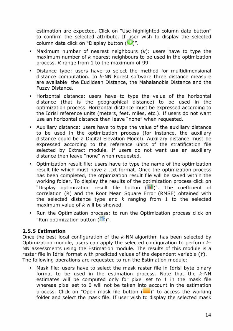
14

estimation are expected. Click on “Use highlighted column data button” to confirm the selected attribute. If user wish to display the selected column data click on “Display button ( )”.

• Maximum number of nearest neighbours (k): users have to type the maximum number of k nearest neighbours to be used in the optimization process. K range from 1 to the maximum of 99.

• Distance type: users have to select the method for multidimensional distance computation. In k-NN Forest software three distance measure are available: the Euclidean Distance, the Mahalanobis Distance and the Fuzzy Distance.

• Horizontal distance: users have to type the value of the horizontal distance (that is the geographical distance) to be used in the optimization process. Horizontal distance must be expressed according to the Idrisi reference units (meters, feet, miles, etc.). If users do not want use an horizontal distance then leave “none” when requested.

• Auxiliary distance: users have to type the value of the auxiliary distance to be used in the optimization process (for instance, the auxiliary distance could be a Digital Elevation Model). Auxiliary distance must be expressed according to the reference units of the stratification file selected by Extract module. If users do not want use an auxiliary distance then leave “none” when requested.

• Optimization result file: users have to type the name of the optimization result file which must have a .txt format. Once the optimization process has been completed, the otpimization result file will be saved within the working folder. To display the results of the optimization process click on “Display optimization result file button ( )“. The coefficient of correlation (R) and the Root Mean Square Error (RMSE) obtained with the selected distance type and k ranging from 1 to the selected maximum value of k will be showed.

• Run the Optimization process: to run the Optimization process click on “Run optimization button ( )”.

2.5.5 Estimation Once the best local configuration of the k-NN algorithm has been selected by Optimization module, users can apply the selected configuration to perform k-NN assessments using the Estimation module. The results of this module is a raster file in Idrisi format with predicted values of the dependent variable (Y). The following operations are requested to run the Estimation module:

• Mask file: users have to select the mask raster file in Idrisi byte binary format to be used in the estimation process. Note that the k-NN estimates will be computed only for pixel set to 1 in the mask file whereas pixel set to 0 will not be taken into account in the estimation process. Click on “Open mask file button ( )” to access the working folder and select the mask file. If user wish to display the selected mask

15

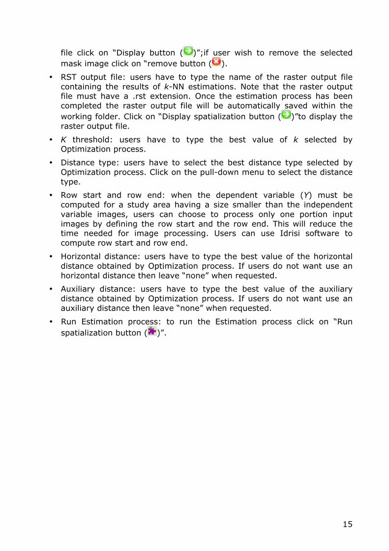
file click on “Display button ( )”;if user wish to remove the selected mask image click on “remove button ( ).

• RST output file: users have to type the name of the raster output file containing the results of k-NN estimations. Note that the raster output file must have a .rst extension. Once the estimation process has been completed the raster output file will be automatically saved within the working folder. Click on “Display spatialization button ( )”to display the raster output file.

• K threshold: users have to type the best value of k selected by Optimization process.

• Distance type: users have to select the best distance type selected by Optimization process. Click on the pull-down menu to select the distance type.

• Row start and row end: when the dependent variable (Y) must be computed for a study area having a size smaller than the independent variable images, users can choose to process only one portion input images by defining the row start and the row end. This will reduce the time needed for image processing. Users can use Idrisi software to compute row start and row end.

• Horizontal distance: users have to type the best value of the horizontal distance obtained by Optimization process. If users do not want use an horizontal distance then leave “none” when requested.

• Auxiliary distance: users have to type the best value of the auxiliary distance obtained by Optimization process. If users do not want use an auxiliary distance then leave “none” when requested.

• Run Estimation process: to run the Estimation process click on “Run spatialization button ( )”.

16

3. Tutorial The Tutorial has been designed to get in confidence with the use of k-NN Forest software. The Tutorial’s dataset consist of 40 field survey units, six multispectral satellite bands and the forest-non forest map. The following files are available within the folder named Tutorial:

• L7b1.rst, L7b2.rst,........., L7b7.rst: these raster files are the six multispectral bands of the Landsat 7 ETM+ satellite (except band 6);

• surveyunits.rst: this is the raster file with the location of 40 field survey units; each pixel is identified with an ID equal to the identifier of the corresponding survey unit; background pixels are set equal to 0.

• surveyunits.dbf: this is the survey units database (in .dbf format) containing the following information for each survey unit: the identifier of the unit (Id) and the measured forest growing stock volume (in cubic meter per hectare);

• mask.rst: this raster file is the forest-non forest map where pixel set to 1 are forested area and pixel set to 0 are non forested area.

The objective of the following exercise is the estimation of the forest growing stock volume using the k-NN Forest software and the Tutorial’s dataset. 3.1 Setting up k-NN Forest To start with k-NN Forest, double click on k-NN Forest application icon in the k-NN Forest Program Folder. Idrisi will automatically loaded. Set the folder named Tutorial as working folder using Idrisi. Select the Set up module and set the maximum number of the independent variable equal to 6 as the number of the available Landsat multispectral bands. Once the number of independent variables has been set equal to 6, save the project using the file menu or the tools bar icons. Call the project “Exercise1” and save it within the folder Tutorial. Then click on Set button and choose “Si” both to restart the application and save your work (Figure 3).

Figure 3. The Set up module.

17

3.2 Extract multispectral features Select Extract module to extract multispectral features from satellite bands for each of the 40 field survey units. First choose the Dependent variable containing the location of the field survey units. To do this click on the orange button on the upper left side and select the raster data file named surveyunits.rst from the working folder (Figure 4). Once the dependent variable has been selected one message in red tells you that the dependent variable file contains 40 survey units. Click on the green button on the upper right side to display the selected dependet variable file with Idrisi (Figure 5).

Figure 4. Selection of the Dependent variable by Extract module.

Figure 5. Visualization of the selected dependent variable.

18

Leave “stratification by1” as the default. Because the maximum number of independent variables has been set equal to 6 by the Set up module, 6 independent variables can be selected by Extract module to extract multispectral features of the field survey units. Click on the orange button on the left side to select the first independent variable and select the raster data file named L7B1.rst, which correspond to the blue band (band 1) of the Landsat 7 ETM+ satellite (remember that independent variables must be raster files in byte binary format; if this is not the case, you can convert the data type using Idrisi with the module named Convert). Repeat the selection procedure for the remaining 5 multispectral bands (L7B2.rst, L7B3.rst, L7B4.rst, L7B5.rst, L7B7.rst). For each independent variable choose Minimum as feature extraction type by using the pull-down menu (Figure 6). Click on the green button on the left side to display the near-infrared band (L7B4.rst) in grey scale (Figure 7).

Figure 6. Selection of the independent variables and definition of the feature extraction type by

Extract module. Now you are ready to extract multispectral features for each field survey unit. To run Extract module click on the button on the upper right side ( ). When the extraction process has been finished a window will appear asking you to type the name for the statistics data file in .txt format which will contain the extracted features. The default name is statistic_data.txt (Figure 8). Leave the default name and click on the OK button to save the statistic data file within the working folder. Go to the working folder and open the statistic data file. First row of the statistic data file contains the following information (from left to right): the number of independent variable (6 multispectral Landsat bands); if a

1 “Stratification file” is an optional auxiliary variable. You must use an auxiliary variable like a Digital Elevation Model if you wish use an auxiliary distance in the Optimization module.

19

stratification data file has been selected (1 if yes, 0 if not); the number of field survey units of the reference set (40 units). Next rows contain statistic data extracted for each survey unit. First column represents the identifier of the field survey units. Second and third columns are the X and Y coordinate of the field survey units. Next columns contain statistic data extracted from independent variables (the DNs from 6 multispectral bands) (Figure 9).

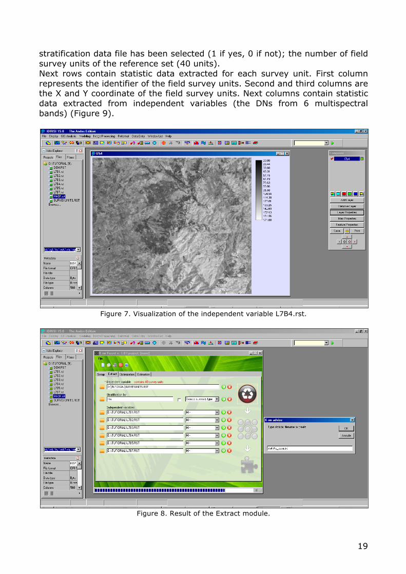
Figure 7. Visualization of the independent variable L7B4.rst.

Figure 8. Result of the Extract module.

20

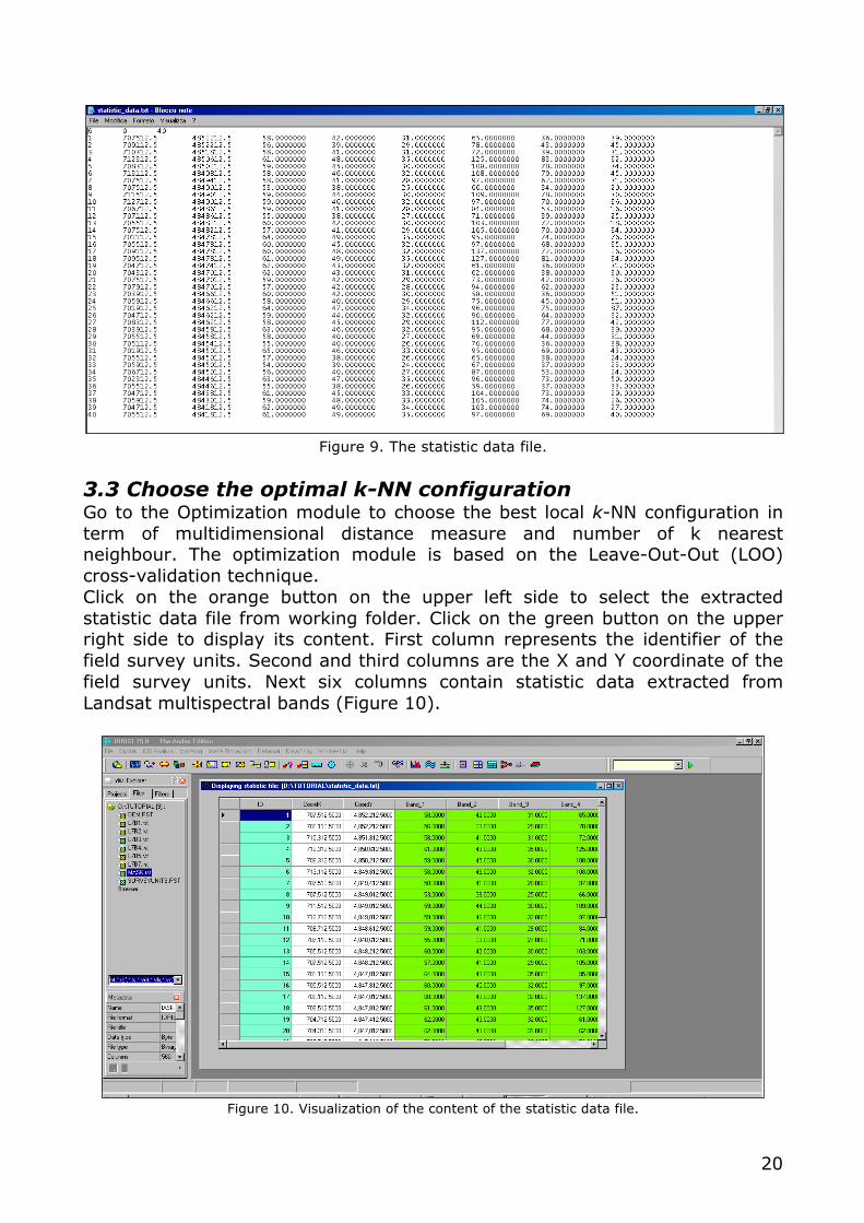
Figure 9. The statistic data file.

3.3 Choose the optimal k-NN configuration Go to the Optimization module to choose the best local k-NN configuration in term of multidimensional distance measure and number of k nearest neighbour. The optimization module is based on the Leave-Out-Out (LOO) cross-validation technique. Click on the orange button on the upper left side to select the extracted statistic data file from working folder. Click on the green button on the upper right side to display its content. First column represents the identifier of the field survey units. Second and third columns are the X and Y coordinate of the field survey units. Next six columns contain statistic data extracted from Landsat multispectral bands (Figure 10).

Figure 10. Visualization of the content of the statistic data file.

21

Close the statistic data file and click on the orange button on the left side to select the survey units database (in .dbf format) named surveyunits. Click on the first green button on the right side to display its content: for each field survey unit the ID and the measured forest growing stock volume (in m3ha-1) are showed. Double click on a cell under “Volume” column to highlight the Volume column data (the selected column will appear hilighted in blue color) then click on button “use highlighted column data” (Figure 11). Note that the highlighted column represents the dependent variable Y for which k-NN estimation are expected. Click on the second green button on the right side to display the selected column data. Set the maximum number of nearest neighbour (k) equal to 20 then use the pull-down menu to choose Euclidean (ED) as multidimensional distance measure type. Type the name of the optimization result file and call it LOO_ED.txt. The result file will be saved within the working folder. Leave horizontal2 and auxiliary3 distance set to “none” as by default then click on the button to run the Optimization module (Figure 12).

Figure 11. Visualization of the survey units database. Column highlighted in blue is the selected dependent variable (forest growing stock volume in m3ha-1) for which k-NN

estimations are expected.

2 The horizontal distance is a geographical distance that can be used as auxiliary parameter to select the k nearest neighbour. Horizontal distance must be expressed according to the Idrisi reference units (meters, feet, miles, etc.). 3 The auxiliary distance is an auxiliary variable like a Digital Elevation Model that can be used to select the k nearest neighbour. Auxiliary distance must be expressed according to the reference units of the stratification file selected by Extract module (see chapter 3.2).

22

Figure 12. Visualization of the Optimization module.

A window will appear with the results of the LOO in term of coefficient of correlation (R) and Root Mean Square Error (RMSE) (Figure 13). Press enter to exit the window then click on the button to graph R and RMSE obtained with the Euclidean distance and k values ranging from 1 to 20 (Figure 14).

Figure 13. List of the LOO results achieved with the Euclidean Distance and k values ranging

from 1 to 20. Additional results produced by LOO are:

1) The value of the optimal k. Optimal k is chosen by k-NN Forest as follows:, the difference (in percentage) between the RMSE obtained with

23

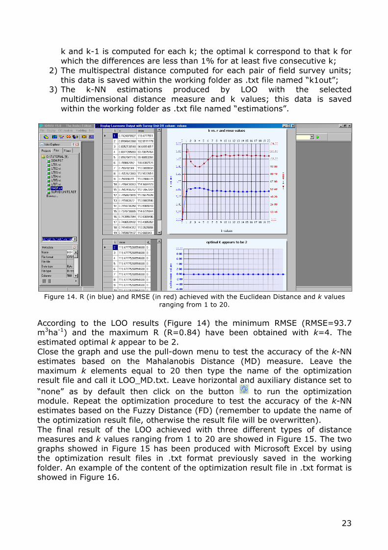
k and k-1 is computed for each k; the optimal k correspond to that k for which the differences are less than 1% for at least five consecutive k;

2) The multispectral distance computed for each pair of field survey units; this data is saved within the working folder as .txt file named “k1out”;

3) The k-NN estimations produced by LOO with the selected multidimensional distance measure and k values; this data is saved within the working folder as .txt file named “estimations”.

Figure 14. R (in blue) and RMSE (in red) achieved with the Euclidean Distance and k values

ranging from 1 to 20. According to the LOO results (Figure 14) the minimum RMSE (RMSE=93.7 m3ha-1) and the maximum R (R=0.84) have been obtained with k=4. The estimated optimal k appear to be 2. Close the graph and use the pull-down menu to test the accuracy of the k-NN estimates based on the Mahalanobis Distance (MD) measure. Leave the maximum k elements equal to 20 then type the name of the optimization result file and call it LOO_MD.txt. Leave horizontal and auxiliary distance set to “none” as by default then click on the button to run the optimization module. Repeat the optimization procedure to test the accuracy of the k-NN estimates based on the Fuzzy Distance (FD) (remember to update the name of the optimization result file, otherwise the result file will be overwritten). The final result of the LOO achieved with three different types of distance measures and k values ranging from 1 to 20 are showed in Figure 15. The two graphs showed in Figure 15 has been produced with Microsoft Excel by using the optimization result files in .txt format previously saved in the working folder. An example of the content of the optimization result file in .txt format is showed in Figure 16.

24

Figure 15. R and RMSE (in m3ha-1) achieved with three different types of distance measures

(ED: Euclidean Distance; FD: Fuzzy Distance; MD: Mahalanobis Distance) and k values ranging from 1 to 20.

Figure 16. Example of the content of the optimization result file obtained with the Euclidean

Distance and k values ranging from 1 to 20.

0.0

0.2

0.4

0.6

0.8

1.0

1 2 3 4 5 6 7 8 9 10 11 12 13 14 15 16 17 18 19 20

K

R

ED FD MD

0

30

60

90

120

150

180

1 2 3 4 5 6 7 8 9 10 11 12 13 14 15 16 17 18 19 20

K

RMSE

ED FD MD

25

According to the LOO results (Figure 15) the best local k-NN configuration has been obtained with the Euclidean Distance and k equal to 4 (R=0.84; RMSE=93.7 m3ha-1). 3.4 k-NN estimation Once the best configuration of k-NN algorithm has been chosen with Optimization module (see chapter 3.3) the k-NN Forest software can be used to perform the final estimation of the parameter of concern (the forest growing stock volume in m3ha-1) over the target forest area. To do this choose the Estimation module and click on the orange button on the upper left side to select the forest-non forest map named mask.rst. Click on the green button on the right side to display the selected mask file. As shown by Figure 17 pixels with a value equal to 1 represent forested are (pixel in red) while pixel with a value equal to 0 are non forested area (pixel in black). k-NN estimations will be computed by k-NN Forest software only for pixels representing forested area. Remember that the mask file must be a byte binary data type (if this is not the case, you can change the data type of the forest-non forest map with Idrisi using the module named Convert).

Figure 17. Visualization of the mask file (pixels in red are forested area, pixel in black are non

forested area). Set k threshold equal to 4 and choose Euclidean Distance as distance type using the pull-down menu. Type the name of the RST output file and call it Volume.rst. Leave all of the other input parameters4 as by default (Figure 18)

4 Row start and row end are two optional parameters that can be used when the dependent variable (Y) must be computed for a study area with a size smaller than the independent variable images; in this case users can choose to process only one portion of the forest non-forest map by defining the row start and the row end. This will reduce the time needed for image processing. Users can use Idrisi software to compute row start and row end. For information about horizontal and auxiliary distances refer to chapter 3.3.

26

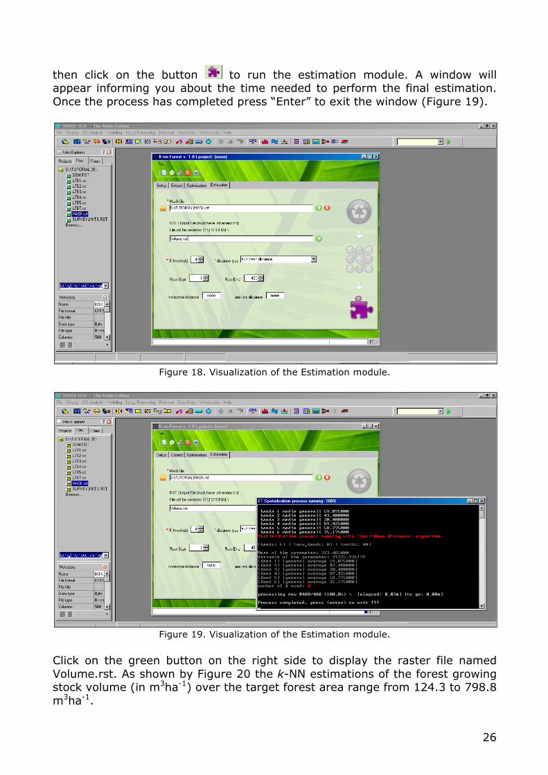
then click on the button to run the estimation module. A window will appear informing you about the time needed to perform the final estimation. Once the process has completed press “Enter” to exit the window (Figure 19).

Figure 18. Visualization of the Estimation module.

Figure 19. Visualization of the Estimation module.

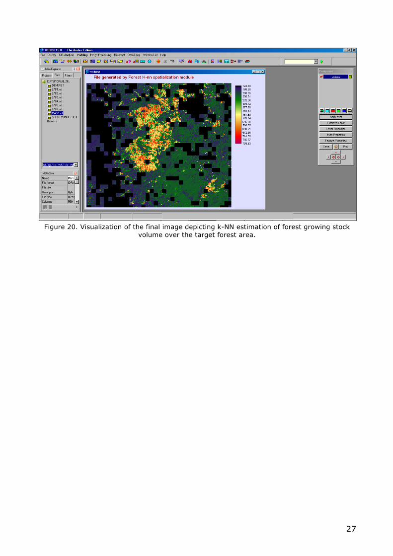
Click on the green button on the right side to display the raster file named Volume.rst. As shown by Figure 20 the k-NN estimations of the forest growing stock volume (in m3ha-1) over the target forest area range from 124.3 to 798.8 m3ha-1.

27

Figure 20. Visualization of the final image depicting k-NN estimation of forest growing stock

volume over the target forest area.