vector4 user’s manual - analysis groupvectoranalysisgroup.com/user_manuals/manual10.pdf · with...
TRANSCRIPT

VecTor4 User’s Manual
T.D. Hrynyk F.J. Vecchio March, 2019

ii
Abstract VecTor4 is a nonlinear finite element analysis program for reinforced concrete shell and slab structures. The program is capable of efficiently analyzing reinforced concrete shell structures at either the component or the system level, while accounting for both geometric and material nonlinearities. The program employs powerful high-order shell elements which can be used to represent structures possessing irregular or curvilinear geometries and structures subjected to highly irregular or non-uniform loading conditions. Cracked reinforced concrete is principally modeled in accordance with the formulations of the Disturbed Stress Field Model (DSFM) (Vecchio 2000), an advanced reinforced concrete behavioral model developed as an extension of the Modified Compression Field Theory (MCFT) (Vecchio and Collins 1986); however, also employs a broad range of supplemental concrete-related mechanical models to capture response mechanisms that fall outside of the original considerations of the DSFM and MCFT (e.g., the influence of confining effects, dilatation, material hysteretic behaviors, consideration of unconventional concrete construction materials, etc.). This User’s Manual is intended to provide guidance regarding the creation of VecTor4 finite element models and supplements several other existing VecTor manuals.
Additional resources related to the pre-processing and post-processing of VecTor4 models include:
Chak, I.N. (2013). “Janus: A Post-Processor for VecTor Analysis Software”, M.S. Thesis, University of Toronto, Department of Civil Engineering, 211 pp., http://vectoranalysisgroup.com/.
Sadeghian, V. (2012). “Formworks-Plus: Improved Pre-Processor for VecTor Analysis Software”, Master’s Thesis, Department of Civil Engineering, University of Toronto, 164 pp., http://vectoranalysisgroup.com/.
Background information related to the development and validation of VecTor4, and the material modeling techniques employed, is provided in the following:
Polak, M.A. and Vecchio, F.J. (1993). “Nonlinear Analysis of Reinforced Concrete Shells”, Department of Civil Engineering, University of Toronto, Publication No. 93-03, December 1993, 195 pp.
Hrynyk, T.D. (2013). “Behavior and Modeling of Reinforced Concrete Slabs and Shells under Static and Dynamic Loads”, Ph.D. Dissertation, University of Toronto, Department of Civil Engineering, 458 pp.
Hrynyk, T.D. and Vecchio, F.J. (2015). “Capturing Out-of-Plane Shear Failures in the Analysis of Reinforced Concrete Shells”, ASCE Journal of Structural Engineering, DOI: 10.1061/(ASCE) ST.1943-541X.0001311.
Wong, P. S., Vecchio, F. J., and Trommels, H. (2013). VecTor2 and Formworks User’s Manual. University of Toronto., http://vectoranalysisgroup.com/.

iii
Table of Contents
1.0 Shell Structure Analysis Program VecTor4 .............................................................................. 1
2.0 VecTor4 Input Files.......................................................................................................................... 3
2.1 Job Files (VECTOR.JOB) ............................................................................................... 4
Loading Data ........................................................................................................................ 4
Analysis Parameters ........................................................................................................... 7
Material Behavior Models ................................................................................................... 8
2.2 Structure Files (##.S4R) ................................................................................................. 9
Structural Parameters ......................................................................................................... 9
Material Specifications ...................................................................................................... 10
Element Incidences ........................................................................................................... 16
Material Type Assignments.............................................................................................. 18
Nodal Coordinates ............................................................................................................. 18
Nodal Restraints ................................................................................................................ 19
2.3 Load Files (##.L4R) ...................................................................................................... 20
Load Case Parameters ..................................................................................................... 20
Loads ................................................................................................................................... 21
2.4 Auxiliary Files (VT4.AUX) ............................................................................................. 24
Solver Parameters: ........................................................................................................... 25
General Analysis Parameters: ......................................................................................... 26
Dynamic Analysis Parameters: ....................................................................................... 26
Tension Softening Parameters: ....................................................................................... 27
3.0 Creating VecTor4 Input Files using FormWorks+ ................................................................. 28
3.1 RC Slab A2 ................................................................................................................... 28
3.2 Creating VecTor4 Model for Slab A2 using FormWorks+ ............................................. 29
Opening the Program ....................................................................................................... 29
Defining JOB Information ................................................................................................. 29
Defining Materials .............................................................................................................. 32
Creating Nodes .................................................................................................................. 34
Creating Elements ............................................................................................................. 35
iv
Assigning Element Material Types ................................................................................. 36
Creating Nodal Restraints ................................................................................................ 37
Assigning Loads ................................................................................................................ 39
3.3 Creation of VecTor4 Input Files .................................................................................... 41
4.0 References ....................................................................................................................................... 42
Appendix A .............................................................................................................................................. 43

1
1.0 Shell Structure Analysis Program VecTor4
VecTor4 is a nonlinear finite element analysis program for reinforced concrete shell and slab structures. The program was originally developed at the University of Toronto (Polak and Vecchio 1993) and has been progressively improved and expanded over the past twenty-five years (e.g., Seracino 1995; Hrynyk 2013; Hrynyk and Vecchio 2014).
The program is capable of efficiently analyzing reinforced concrete shell structures at either the component or the system level, while accounting for both geometric and material nonlinearities. Software program VecTor4 employs powerful high-order shell elements which can be used to represent structures possessing irregular or curvilinear geometries and structures subjected to highly irregular or non-uniform loading conditions. Cracked reinforced concrete is principally modeled in accordance with the formulations of the Disturbed Stress Field Model (DSFM) (Vecchio 2000), an advanced reinforced concrete behavioral model developed as an extension of the Modified Compression Field Theory (MCFT) (Vecchio and Collins 1986); however, also employs a broad range of supplemental concrete-related mechanical models to capture response mechanisms that fall outside of the original considerations of the DSFM and MCFT (e.g., the influence of confining effects, dilatation, material hysteretic behaviors, etc.). Thus, with this approach, the material modeling used in VecTor4 inherently considers the redistribution of internal forces that can occur due to local changes in stiffness arising from cracking or crushing of concrete, yielding of reinforcement, the influence of variable and changing crack widths (including crack slip deformations developed along crack surfaces), and various second-order mechanisms that often contribute significantly to the response of reinforced concrete shell structures.
Perhaps the most notable feature of program VecTor4 is the use of a layered thick-shell element formulation. Unlike typical commercial analysis programs that often require complex finite element meshes that are expensive in terms of preparation and computation, the layered procedure used by VecTor4 has been shown to effectively capture structure response mechanisms (including through-thickness shearing effects) using finite element modeling techniques requiring significantly reduced computational effort. This feature, combined with the advanced behavioral modeling employed, makes VecTor4 somewhat unique and typically much more practical for the investigation of large-scale concrete slab, shell, and planar structures (refer to Figure 1.1a).
The layered shell element, or stacked membrane concept, employed by VecTor4 allows for stiffness variations through the thickness of the element arising from different types of materials (e.g., laminated plates or fabrics, conventional steel reinforcing bars, concrete, etc.) or material nonlinearity to be represented discretely. With the use of appropriate compatibility assumptions to describe the in-plane strain variation through the thickness of the shell (plane sections remain plane, for example), and assumptions pertaining to the out-of-plane shear strain distribution, stress and strain conditions can be evaluated through the thickness of the shell elements with minimal computational effort. Figure 1.1b illustrates the layered shell element concept and assumed strain variations through the thickness of the shell finite elements employed by VecTor4.
Over the past several decades, a significant amount of research has been undertaken to develop cost effective analysis procedures that can be applied to the analysis of RC shell structures under combined membrane forces (Nx, Ny, Nxy), bending moments (Mx, My, Mxy), and out-of-plane shear

2
forces (Vxz, Vyz) (refer to Figure 1.2). VecTor4 is a viable tool for such applications and can be used to gain insight into the response of RC shell structures of different sizes and complexities, under various combined loading scenarios. Perhaps most relevant to the analysis of RC shells, VecTor4 has been shown to provide reliable strength estimates for RC elements under combined in-plane and out-of-plane shear forces and has been shown to be capable of capturing brittle out-of-plane shear failure modes (Hrynyk 2013; Hrynyk and Vecchio 2014; Hrynyk and Vecchio 2016).
(a) candidate RC structures
(b) layered element concept and sectional response conditions
Figure 1.1 – VecTor4 sample modeling applications and layered approach.
Figure 1.2 – VecTor4 layered shell element loading conditions.
local z
local y
localx
Nx Mxy
VxzNxy Mx
NxMxy
NxyMxVxz
VyzNy
Myx
My
Nyx
Nyx
VyzNy
Myx
My

3
2.0 VecTor4 Input Files
This chapter provides an overview of the structure and contents of the input files required to perform a VecTor4 analysis. To supplement the input documentation provided in this manual, input text files for a sample VecTor4 models are provided in Appendix A.
To perform a VecTor4 analysis, at least four input text files are required: a job file (VECTOR.JOB), a structure file (##.S4R), at least one load file (##.L4R), and an auxiliary data file (VT4.AUX). Provided in the same directory as the VecTor4 executable file (VT4.EXE), the program calls upon these input text files to define the finite element model comprising the structure to be analyzed and to specify the analysis and modelling parameters to be considered during the solution procedure. Each of the four types of input text files is prepared according to a predefined template with user-specified data being input using a fill-in-the-blank updating format or, alternatively, may be created using the VecTor4 preprocessor, FormWorks+ (Sadeghian 2012). In the case of manual input file creation/updating, commonly employed text editing programs such TextPad or Microsoft Notepad can be used to update and modify the VecTor4 input files.
For demonstration purposes, the following subsections of this manual will make reference to VecTor4 input files that were developed for the analysis of a RC thin slab specimen tested by Aghayere and MacGregor (1990). Slab specimen A2 had the planar geometry shown in Figure 2.1a and was subjected to combined in-plane axial compression and out-of-plane shear loading conditions. Taking advantage of symmetry, a VecTor4 finite element model consisting of 49 layered shell elements was used to represent a one-quarter region of the test specimen. For simplicity, regular element sizing and nodal spacing was used (refer to Figure 2.2b). Note that additional details regarding the specimen and loading conditions considered in the testing program are available in the original publication presented by Aghayere and MacGregor (1990).
(a) planar geometry of thin slab A2 (b) one-quarter slab model
Figure 2.1 – VecTor4 model of thin slab specimen A2.
610 305
152
1829
152
457 457 152
610305
457457152
Transverse Loading Plates
Roller Supports
P P
P P
P P
P P
X
Y
Z
axis of symmetry (aos)
aos
out-of-plane nodal restraint
out-of-plane nodal load
in-plane nodal loads
- 49 shell elements (7 x 7 grid)
- 225 nodes (15 @ 76.25 mm in each direction)

4
2.1 Job Files (VECTOR.JOB) The job file (VECTOR.JOB) includes input fields to describe the characteristics of the analysis procedure considered and to select material behavior models. The job file is also used to direct the VecTor4 program to the structure file and load files that are to be considered in the analysis. Job Descriptor Data
At the beginning of the job file, information used to document the specific analysis/job is provided (see Figure 2.2).
Figure 2.2 – Job file descriptor data. As shown in Figure 2.2, the first three input lines (Job Title, Job File Name, Date) can be used to document background information related to the job/analysis being performed. Any combination of letters, numbers, and symbols may be used in these lines, provided they conform to the noted character limitations (e.g., 8 char max). Under the subheading STRUCTURE DATA, the Structure Type should always be specified as 4 for analyses performed using VecTor4. The File Name is used to direct the VecTor4 analysis program to the desired structure file (##.S4R) to be used in the analysis. Note that multiple structure files may exist within the same directory as the VT4.EXE program; only the file specified in the File Name field will be considered in the analysis. In the case of slab specimen A2, the structure file is named Struct.S4R. Loading Data
The following section of the job file, identified as LOADING DATA, is used to control the manner in which the applied loads (specified in separate ##.L4R files) for a given analysis change from one load stage to the next (see Figure 2.3). In the case of the VecTor4 analysis for RC slab A2, the program is specified to execute a total of 100 load stages (No. of Load Stages). Data output files (##.A4E files) containing the analysis results and generated for each of the load stages performed will be numbered sequentially, with the load stage numbering starting from 1 (Starting Load Stage No.). Note that, typically, analyses can be stopped and then resumed at a later time by way of a subsequent analysis. In such cases, it may be advantageous to change the Starting Load Stage No. field such that output file numbering continues from the termination of the initial analysis. The Load Series ID field allows the user to specify the naming convention used for

5
generated output files. For example, from the segment of the job file presented in Figure 2.3 for slab A2, the output file summarizing the analytical results generated from the first load stage performed will be identified as ID_01.A4E. The output files are written to the same directory location as the input text files and the VecTor4 analysis program.
Figure 2.3 – Job file Loading Data. Up to five load files (##.L4R files) representing static or dynamic loading events may be considered in a VecTor4 analysis. The load files are specified under the column field with the heading File Name. Note that a NULL entry under the File Name column is used to deactivate a given load case. The load factor fields (Initial, Final, Inc, Typ, Rep, C-Inc) are used to control how the loads comprising the load files are changed from one load stage to the next. In the case of dynamic loading conditions, load factor fields are used to control the increments of the time stepping analysis. Load files consisting of static load types (e.g., concentrated nodal forces/displacements, gravity loads, element surface pressures, etc.) may be applied using monotonic, cyclic, or reversed cyclic loading conditions. Dynamic loads (e.g., base accelerations, user defined impulse time histories, initial mass velocities/accelerations, etc.) however, are fixed in magnitude and are applied according to the data provided in the user generated input load files (##.L4R). Examples of load factor specifications used to consider monotonic, cyclic, and reversed cyclic loading conditions are presented in Figures 2.4a, b, and c, respectively.
The required input comprising the load factor fields consists of: the Initial load value which is used to specify the load multiplier for first load stage performed; the Final load value which is used to specify the maximum load multiplier to use in the case of a monotonic analysis or the multiplier required to achieve the maximum load amplitude for the first cycle comprising a cyclic or reversed cyclic analysis; the Inc load factor is used to specify the load increment that is used from one load stage to the next; the Typ designation is used to specify whether the load file is to be applied as monotonic (Typ = 1), cyclic (Typ = 2), or reversed cyclic (Typ = 3) loading; the Rep value is used to specify the number of cyclic or reversed cyclic cycles to be performed at each amplitude load level; and C-Inc is used to specify the cyclic increment (i.e., the change in load cycle amplitude).
Thus, referring again to Figure 2.3 for the case of the slab specimen A2, it can be seen that two load cases were used. Load Case 1: AXIAL was used to define the constant in-plane axial load that was applied to the slab and, as such, the Initial, Final, and LS-Inc factors for this loading case

6
were set equal to 1.0 resulting in a constant (i.e., non-incremented) load. Load Case 2: SHEAR was used to represent the monotonically-increasing out-of-plane shear loading. In the first load stage, applied out-of-plane shear forces will be multiplied by the Initial factor of 0.0000, and the factor will then be subsequently increased by increments of 0.1000. Thus for example, in the 6th load stage of the analysis, the applied loads will consist of the axial loads comprising Load Case 1 multiplied by a load factor of 1.0000 (i.e., they will remain unchanged) and the out-of-plane shear forces comprising Load Case 2 will be multiplied by a load factor of 0.5000.
(a) monotonic loading condition
(b) cyclic loading condition
(c) reversed cyclic loading condition
Figure 2.4 – Loading Data specifications for different analysis types.

7
Analysis Parameters
Section ANALYSIS PARAMETERS (see Fig. A1.4) is used to specify several global analysis parameters that influence how the analysis procedure operates, outputs data, and stores information.
Figure 2.5 – Job file Analysis Parameters (default values shown). Field Analysis Mode is used to specify whether the analysis involves quasi-static loading
(mode 1), thermal time-stepping (mode 2), a general dynamic analysis (mode 3), or a dynamic analysis using a standardized base acceleration input file (mode 4).
The Seed File Name field is used to direct the analysis program to an existing output binary file, developed from a prior VecTor4 analysis. Thus, with the use of seed files, VecTor4 analyses may typically be stopped and resumed, or a damaged structure state resulting from one VecTor4 analysis may be used as an input condition for the beginning of another VecTor4 analysis.
The Convergence Limit is used to specify the convergence threshold that must be satisfied from one iteration to the next, prior to the analyses continuing to the next load stage. If convergence is not achieved within the Maximum No. of Iterations specified, the analysis will proceed to the next load stage without having satisfied the specified Convergence Limit.
The use of an Averaging Factor is generally recommended to stabilize the numerical solution. An Averaging Factor value less than or equal to 1.0 is required and, as such, this factor is used to over-relax the nonlinear solution, resulting in a smoothing of the results from iteration to iteration of the analysis.
The Convergence Criteria specifies the parameter used to monitor the change in the analytical solution from one iteration to the next. As a default option, VecTor4 estimates convergence based on the change in the nodal displacements and rotations from one iteration to the next. [criteria 1 = weighted secant stiffness; criteria 2 = weighted displacements; criteria 3 = maximum displacements]
The Results File Type field in this section of the job file is used to specify the type and frequency of the output files generated over the course of a VecTor4 analysis. Typically, providing the output analysis results, for each load stage, as readable text is most useful for post-processing of results; however, there are also options to print binary file solution output

8
which is required to resume an analysis. [type 1 = ASCII and binary file output for all load stages; type 2 = only ASCII files for all load stages; type 3 = only binary file output for all load stages; type 4 = ASCII and binary file output for only the last load stage.
Note that all of the analysis parameters shown in Figure 2.5 represent default/recommended values for typical VecTor4 quasi-static (monotonic and cyclic) analyses.
Material Behavior Models
The last section of the job file is the MATERIAL BEHAVIOR MODELS section. Within this section, the user can choose from several available material/behavioral models. However, it should be noted that a set of ‘default’ material and structure behavioral models have been predefined in VecTor4. The default models have been established on the basis of prior validation studies involving VecTor4 and other VecTor software analysis programs, and result in what is believed to be a balanced approach resulting in reasonable solution accuracy and solution stability, under typical loading and analysis scenarios.
The use of default modelling options are recommended and are applicable for most analyses; however, VecTor4 does support a wide range of non-default behavioral models which may be advantageous in the analysis of certain structures possessing atypical details or loading conditions, or in cases where the user is investigating the influence of a specific response mechanism. A complete listing and summarized descriptions of the available material and structure behavioral models are provided in Wong et al. (2013). The models and analysis options which comprise the default material models for VecTor4 are summarized below in Table 2.1.
Table 2.1 - VecTor4 default behavioral models.
Concrete Models Reinforcement Models
Compression Base Curve : Hognestad (parabola) Hysteretic Response : Bauschinger (Seckin) Compression Post-Peak : Modified Park-Kent Dowel Action : Tassios (crack slip) Compression Softening : Vecchio 1992-A Tension Stiffening : Modified Bentz Analysis Options Tension Softening : Linear Shear Analysis Mode : Parabolic Shear Strain FRC Post-Crack Tension : SDEM Strain History : Considered 2 Confined Strength : Kupfer / Richart Strain Rate Effects : CEB/Malvar-Crawford2 Dilatation : Variable - Kupfer Structural Damping : Rayleigh 2 Cracking Criterion : Mohr-Coulomb (stress) Geometric Nonlinearity : Considered Crack Stress Calculation : Basic (DSFM/MCFT) Crack Allocation : Uniform Crack Width Check : Crack Limit (agg/2.5) 2 default options for VecTor4 dynamic analysis Crack Slip Calculation : Walraven Hysteretic Response : Nonlinear w/ Plastic Offsets
Specification of the above-noted default material behavior models, done by way of text file input in the Vector.JOB file, is shown in Figure 2.6.

9
Figure 2.6 – Job file Material Behavior Models (default values shown).
2.2 Structure Files (##.S4R) The VecTor4 structure file (##.S4R) contains input fields to specify material properties, including reinforcement configurations and ratios, input fields to describe the geometry of the structure being modeled, and fields to define the finite element meshing and boundary conditions comprising the model. As was the case for discussion pertaining to the job file, the structure file STRUCT.S4R which was used in the analysis of RC slab A2 tested by Aghayere and MacGregor (1990) is again used for illustration in the following section. Structural Parameters
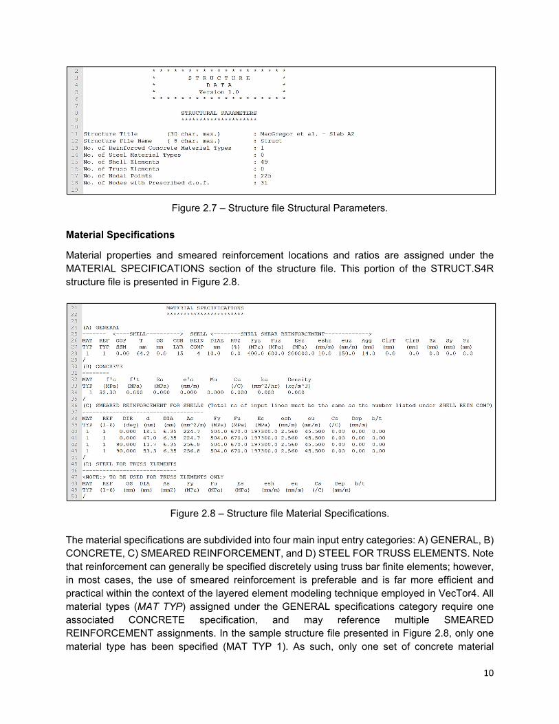
At the top of the VecTor4 structure file, the STRUCTURAL PARAMETERS (see Figure 2.7) section is used to input information regarding the finite element model as well information used to document the analysis job.
The first two lines of the file, listed as Structure title and Structure file name, are used for documentation purposes only. As such, any combination of characters, symbols, and numbers may be entered in these fields provided they conform to the noted maximum character limitation (e.g., 8 char. max. for Structure file name input). The remaining six lines are used to specify the number of material types, elements (for each type of element used), nodal points, and restrained nodes. For example, in the case of RC slab A2, the VecTor4 model created (refer to Figure 2.1) consisted of 49 layered shell elements, 225 nodes (31 of which have some type of imposed restraint to simulate boundary conditions), and 1 material type. Note that for this particular model, no truss elements were used and, therefore, no steel material types (material definition exclusive to truss elements) were defined.
10
Figure 2.7 – Structure file Structural Parameters. Material Specifications
Material properties and smeared reinforcement locations and ratios are assigned under the MATERIAL SPECIFICATIONS section of the structure file. This portion of the STRUCT.S4R structure file is presented in Figure 2.8.
Figure 2.8 – Structure file Material Specifications. The material specifications are subdivided into four main input entry categories: A) GENERAL, B) CONCRETE, C) SMEARED REINFORCEMENT, and D) STEEL FOR TRUSS ELEMENTS. Note that reinforcement can generally be specified discretely using truss bar finite elements; however, in most cases, the use of smeared reinforcement is preferable and is far more efficient and practical within the context of the layered element modeling technique employed in VecTor4. All material types (MAT TYP) assigned under the GENERAL specifications category require one associated CONCRETE specification, and may reference multiple SMEARED REINFORCEMENT assignments. In the sample structure file presented in Figure 2.8, only one material type has been specified (MAT TYP 1). As such, only one set of concrete material
11
properties is specified under the CONCRETE specification. In this case, material type 1 (MAT TYP 1) has four associated in-plane smeared reinforcement assignments, two for each mat of steel comprising the RC slab.
Brief definitions for each of the variables used in the MATERIAL SPECIFICATION section of the structure file are provided below. The listed variables have been separated according to the categories used in the VecTor4 structure file: GENERAL:
MAT TYP (material type): an integer used to identify the shell element material types considered in a given analysis. Shell element material types are ordered sequentially from 1 to n, where n is the number of material types considered in the analysis.
REF TYP (reference type): an integer used to describe the type of shell element used in the analysis. In VecTor4, the REF TYP is always equal to 1.
OOP SSM (out-of-plane shear strain multiplier): a modification factor used to reduce the out-of-plane shear deformations of shell elements. This factor can be used to approximately account for beneficial confining effects in regions of a structure immediately surrounding concentrated loads and reactions (i.e., disturbed regions). The OOP SSM factor must be a positive real number less than or equal to one. When the OOP SSM factor is set equal to 0.0, the influence of confining effects are considered in the analysis for all elements comprising the MAT TYP, and the OOP SSM factors to be applied to each shell element Gaussian integration point are computed automatically on the basis of the locations of the out-of-plane loads and restraints, and structure geometry. Alternatively, user-specified OOP SSM factors (between 0.0 and 1.0) may be employed. To neglect through-thickness confining effects within the layered shell elements, the OOP SSM factor should set equal to 1.00.
T (shell element thickness): the average through-thickness dimension of the layered shell element. Specified in units of mm. [Note: this thickness is only used when model geometry is defined using centerline nodal coordinates.]
OS (centerline offset): element offset measured from the location of the nodes (typically at the mid-height of the element). A negative offset is toward the element bottom surface. Specified in units of mm.
CON LYR (concrete layers): an integer specifying the number of concrete layers to consider for the layered shell elements comprising the MAT TYP. For structures subjected to out-of-plane loads/deformations, the minimum number of concrete layers is 2. The maximum number of concrete layers permitted in a VecTor4 analysis is version dependent.
REIN COMP (reinforcement components): an integer specifying the number of reinforcement components/layers associated with the MAT TYP. The maximum number of reinforcement layers associated with each MAT TYP is version dependent.
DiaZ (diameter of out-of-plane steel reinforcing bars): a positive real number. Specified in units of mm.

12
ROZ (z): the out-of-plane reinforcement ratio for elements assigned to the MAT TYP. For shell elements containing no through-thickness shear reinforcement, ROZ should be set equal to zero. Specified in %.
Fyz: the yield stress of the out-of-plane reinforcement associated with the MAT TYP. Specified in units of MPa.
Fuz: the ultimate tensile strength of the out-of-plane reinforcement associated with the MAT TYP. Specified in units of MPa.
Esz: the modulus of elasticity for the out-of-plane reinforcement assigned to the MAT TYP. Specified in units of MPa.
eshz: the strain corresponding to the onset of strain hardening for the out-of-plane reinforcement. Specified in units of millistrain (mm/mm x 10-3).
euz: the strain corresponding to the ultimate tensile strength (Fuz) of the out-of-plane reinforcement. Specified in units of millistrain (mm/mm x 10-3).
Agg (aggregate): the maximum nominal aggregate size. Specified in units of mm.
ClrT (clear cover top): the clear cover provided on the top surface of the shell elements assigned to the MAT TYP. In the case of conventional RC material modeling, the clear cover is used to determine which concrete layers contain smeared out-of-plane shear reinforcement and which layers are to be treated as unreinforced (in the out-of-plane direction) concrete cover layers. Specified in units of mm.
ClrB (clear cover bottom): the clear cover provided on the bottom surface of the shell elements assigned to the MAT TYP. [see note above for ClrT regarding usage]. Specified in units of mm.
Sx: a real number used to specify the mean stabilized crack spacing in the local x-direction. If an input value of 0.0 is specified, VecTor4 automatically computes the crack spacing according to the crack allocation behavioral model assigned in the VECTOR.JOB file. Specified in units of mm.
Sy: a real number used to specify the mean stabilized crack spacing in the local y-direction. If an input value of 0.0 is specified, VecTor4 automatically computes the crack spacing according to the crack allocation behavioral model assigned in the VECTOR.JOB file. Specified in units of mm.
Sz: a real number used to specify the mean stabilized crack spacing in the local z-direction (the through-thickness direction). If an input value of 0.0 is specified, VecTor4 automatically computes the crack spacing according to the crack allocation behavioral model assigned in the VECTOR.JOB file. Specified in units of mm.

13
CONCRETE:
MAT TYP (material type): an integer used to link concrete property assignments to the shell element attributes specified for the MAT TYP in the GENERAL section specifications.
f’c: the peak uniaxial concrete compressive stress. Specified in units of MPa.
f’t: the peak concrete tensile strength under direct tension. If an input value of 0.0 is specified,
VecTor4 automatically computes the direct tensile strength as ' 0.33 't cf f . Specified in
units of MPa.
Ec: the concrete modulus of elasticity. If an input value of 0.0 is specified, VecTor4
automatically computes the concrete modulus as 2 ' 'c c cE f . Specified in units of MPa.
e’c: the concrete strain associated with the peak compressive stress (f’c). If an input value of
0.0 is specified, VecTor4 automatically computes this strain value as ' 1.8 0.0075 'c cf .
Specified in units of millistrain (mm/mm x 10-3).
Mu (v): Poisson’s ratio for concrete. If an input value of 0.0 is specified, VecTor4 assumes an initial Poisson ratio of 0.15.
Cc: the coefficient of thermal expansion for concrete. This coefficient is used in VecTor4 analyses considering thermal loads. If an input value of 0.0 is specified, VecTor4 assumes a thermal expansion value of 12 x 10-6 / oC. Specified in / oC.
kc: the thermal diffusivity value. This value is used in VecTor4 analyses considering thermal loads. If an input value of 0.0 is specified, VecTor4 assumes a diffusivity value of 4,320 mm2 / hour. Specified in mm2 / hour.
Density: density of reinforced concrete. This value represents the average density from the combined concrete and internal reinforcement and is employed in the computation of applied gravitational loads and in defining the nodal masses used in dynamic analyses. If an input value of 0.0 is specified, VecTor4 automatically considers a reinforced concrete density value of 2,400 kg / m3. Specified in kg / m3.
SMEARED REINFORCEMENT FOR SHELLS (in-plane reinforcement):
MAT TYP (material type): an integer used to link the reinforcement component/layer to the shell element attributes specified for the MAT TYP in the GENERAL section specifications.
REF (reference type): an integer used to specify the type of in-plane reinforcement. The following smeared reinforcement reference types are currently available in VecTor4:
1) Ductile Steel Reinforcement (tension and compression) 2) Prestressing Steel (tension and compression) 3) Ductile Steel Reinforcement (tension only) 4) Ductile Steel Reinforcement (compression only)
14
5) Externally Bonded FRP Plate/Fabric 6) Steel Fibre Reinforced Concrete 7) Steel Skin Plate (used for steel-concrete composite analyses)
DIR (reinforcement direction): specifies the in-plane orientation of smeared reinforcement, relative to the local-x axis of the shell element. DIR is specified in units of degrees and is taken with respect to the local x-axis. In the case of REF type 6, this field is used to specify the fibre volume ratio, in %. For REF type 7, the reinforcement direction is not used and may be specified as 0.0.
d (depth): the depth to the center of the reinforcement layer from the top surface of the concrete. In the case of SC construction, d is the depth to the steel faceplate layer from the top concrete surface. Specified in units of mm and not applicable to REF type 6.
DIA (diameter): the diameter of the reinforcing bar (or steel fibre). Specified in units of mm. **Note that in SC analyses (REF type 7), DIA represents the Poisson ratio for the steel faceplate.
As (area of steel): the area of smeared in-plane reinforcement. Specified in units of mm2 / m. For REF type 6, this field is used to specify the steel fibre length (specified in units of mm). For steel-concrete composite analyses (REF type 7), As represents the thickness of the steel faceplate (specified in units of mm).
Fy: the yield stress of the in-plane reinforcement component. Specified in units of MPa.
Fu: the ultimate strength of the in-plane reinforcement component. Specified in units of MPa.
Es: the modulus of elasticity for the in-plane reinforcement component. Specified in units of MPa.
esh: the strain corresponding to the onset of strain hardening for the in-plane reinforcement component. Specified in units of millistrain (mm/mm x 10-3).
eu: the strain corresponding to the ultimate tensile strength (Fu) of the in-plane reinforcement component. Specified in units of millistrain (mm/mm x 10-3).
Cs: the coefficient of thermal expansion for steel. If an input value of 0.0 is specified, VecTor4 assumes a thermal expansion value of 10 x 10-6 / oC. Specified in / oC.
Dep (): steel prestrain used to accommodate steel prestress forces. Specified in units of millistrain (mm/mm x 10-3).
b/t (or L/d): in the case of conventional reinforcing bars, this is the ratio of the unsupported bar length (e.g., length between supporting stirrups) to the reinforcing bar diameter. In the case of steel skin plate construction (SC construction), this is the ratio of the average orthogonal anchor stud spacing to the thickness of the steel face plate.

15
STEEL FOR TRUSS ELEMENTS (used for truss bar elements):
MAT TYP (material type): an integer used to identify the truss bar element material types considered in a given analysis. Truss bar material types are ordered sequentially from 1 to n, where n is the number of material types considered in the analysis. Note that these material type designations are independent of those defined above for shell elements.
REF (reference type): an integer used to specify the type of truss bar response. The following truss bar element reinforcement reference types are currently available in VecTor4:
1) Ductile Steel Reinforcement (tension and compression) 2) Prestressing Steel (tension and compression) 3) Ductile Steel Reinforcement (tension only) 4) Ductile Steel Reinforcement (compression only) 5) Linear Elastic (tension only) [not currently available in FW+] 6) Linear Elastic (compression only) [not currently available in FW+]
OS (truss bar geometric offset): truss bar element offset measured from the location of the
nodes (typically at the mid-height of the element). A negative offset is used to specify a truss bar depth from the centerline, toward the element bottom surface. Specified in units of mm.
DIA (diameter): the diameter of the truss/reinforcing bar. Specified in units of mm.
As (area of steel): the cross sectional area of the truss bar element. Specified in units of mm2.
Fy: the yield stress of the truss bars associated with the governing MAT TYP. Specified in units of MPa.
Fu: the ultimate tensile stress of the truss bars associated with the governing MAT TYP. Specified in units of MPa.
Es: the modulus of elasticity for the truss bars associated with the governing MAT TYP. Specified in units of MPa.
esh: the strain corresponding to the onset of strain hardening for the truss bars associated with the governing MAT TYP. Specified in units of millistrain (mm/mm x 10-3).
eu: the strain corresponding to the ultimate tensile strength (Fu) of the truss bars associated with the governing MAT TYP. Specified in units of millistrain (mm/mm x 10-3).
Cs: the coefficient of thermal expansion for the truss bars associated with the governing MAT TYP. If an input value of 0.0 is specified, VecTor4 assumes a thermal expansion value of 10 x 10-6 / oC. Specified in / oC.
Dep (): steel prestrain used to accommodate steel prestress forces. Specified in units of millistrain (mm/mm x 10-3).
b/t: this is the ratio of the unsupported bar length (e.g., length between supporting stirrups) to the truss bar diameter.

16
Element Incidences
Two types of finite elements are available in program VecTor4: layered heterosis shell elements and truss bar finite elements. Shell elements are composite type elements that are used to represent the combinations of concrete, smeared in-plane steel contributions consisting of internal reinforcing bars or external face plates, and smeared out-of-plane (through-thickness) reinforcement contributions. Truss bar elements can be used to discretely represent in-plane reinforcing steel components or to serve as springs or restraining elements. Typically, the layered shell formulation can be used to adequately represent reinforcement contributions and usually results in reduced computational cost.
The heterosis shell element employed by VecTor4 is a 9-node element with 42 degrees-of-freedom (three translations and two rotations for each of the eight perimeter nodes, two rotations for the central ninth node). The nine nodal points comprising each shell element must be specified using the global nodal numbering scheme pertaining to the finite element model. To specify the nodes associated with the shell elements, element nodes must be defined in a counter-clockwise fashion with respect to the top surface of the layered element and the first node (i.e., node #1) used in defining the shell element must correspond to one of the four corner nodes comprising the element.
The required element node specification procedure is illustrated in Figure 2.9. However note that element nodal numbering scheme may commence from any corner node comprising the shell element and that typical VecTor4 finite element meshes will usually result in non-consecutive nodal numbering when defining the nine local incidence nodes associated with each shell element.
Figure 2.9 – Heterosis element node specification (Sadeghian 2012).
The global nodes associated with each shell element are specified in the ELEMENT INCIDENCES section of the VecTor4 structure input file (see Figure 2.10). The global node numbers associated with the nine nodes comprising a given shell element (ELMT) are specified using the INC1 through INC9 input fields, according to the specification procedure illustrated in Figure 2.9. The nodal specification procedure shown must be provided for each shell element

17
comprising the finite element model. Note however, in cases where a regular and patterned grid of shell elements is used, the element incidence information for multiple elements can often be specified using a single input line. For example, in the case of RC slab A2, which consisted of a of a grid of 7 layered shell elements and was used to represent one-quarter of the slab test specimen, the regular nodal numbering employed in this case allowed nodal incidence information for all 49 shell elements to be specified in a single line of input. From Figures 2.10 and 2.11, it can be seen that the nine global node numbers pertaining to element 1 (the bottom-left element shown in Figure 2.11) are specified in the INC1 through INC9 fields, and are followed by eight additional user input entries: #ELMT, d(ELMT), d(INC1), and d(INC4). Input field #ELMT pertains to the number of connecting shell elements in a row or column that possess the same nodal numbering pattern as element ELMT (element 1 in this case); the d(ELMT) input is used to specify the change in the element number along the row or column of shell elements being specified; and similarly, d(INC1) and d(INC4) are used to specify the change in global node numbers along the row or column of shell elements pertaining to INC1 and INC4, respectively. Thus, the use of the eight additional input fields following the nine nodal incidences permit the definition of regular planar grids of heterosis shell elements, using a single line of text input.
Figure 2.10 – Structure file element connectivity specifications.
Figure 2.11 – VecTor4 finite element mesh; plan view and nodal numbering for slab A2.

18
A similar set of input fields exist for the truss bar element incidence specifications. However, unlike the heterosis shell elements employed by VecTor4, there is no required node specification procedure for truss bar elements. INC1 and INC2 are used to specify the two global nodes comprising each truss bar element. Similar patterning procedures can be employed to specify multiple truss bar elements defined by regular nodal numbering, using a single line of input. In the case of RC slab A2, no truss bar elements were used in the model (refer to Figure 2.10). Material Type Assignments
Following the ELEMENT INCIDENCES specifications is the section of the structure file that is used to specify MATERIAL TYPE ASSIGNMENTS. In this section, previously defined material types (MAT TYP) are assigned to corresponding shell and truss bar elements. Note that all finite elements used in a VecTor4 model must be assigned a material type; however, not all material types specified in the VecTor4 structure file need to be used in the material type assignments.
As shown in Figure 2.12, only three input fields are required for the material type assignments: ELMT, MAT, and ETYPE. The MAT field entry is used to specify the shell or truss bar material type corresponding to element # ELMT. The ETYPE is used to define what type of finite element is being used for each ELMT. Currently, ETYPE=1 is to be used for shell element assignments and ETYPE=3 us to be used for truss bar finite elements. Using a methodology similar to that described previously, an additional two input fields (#ELMT and d(ELMT)) can be specified such that multiple elements can be assigned to a single material type, by way of a single line of text input. In the case of RC slab A2, it can be seen that all 49 shell elements are assigned as material (MAT) type 1, and element type (ETYPE) 1, using a single line of input.
Figure 2.12 – Structure file Material Type Assignment. Nodal Coordinates
The COORDINATES section of the structure file is used to specify the location of all nodal points used in a VecTor4 finite element model, in three-dimensional space. Two types of coordinate entry formats can be employed: i) format (TYPE) 1 requires that two coordinate locations, used to describe the top surface and bottom surface of the element, are specified for each nodal point (refer to Figure 2.9), and ii) format (TYPE) 2 requires that only one three-dimensional coordinate location be specified for each node and thus, only the centerline geometry of the shell structure is described by the nodal coordinate specifications. TYPE 2 coordinates (shell element centerline coordinates) can only be used to specify uniform planar shell structure geometry. TYPE 1 coordinates are general and can be used to describe any valid VecTor4 shell structure geometry.
The number of COORDINATE input fields differs depending on the coordinate specification type/format. As shown in Figure 2.13, TYPE 2 (centerline) coordinates were used to specify the

19
locations of the nodes pertaining to RC slab A2. In this case, the node number (NODE) is followed by the coordinate type (TYPE), and then three real numbers that are used to specify the location of the node in X-Y-Z space. As the nodes in this model are geometrically spaced at regular intervals, the three-dimensional coordinates for multiple nodes have been specified using a single line of input. In this example, nodal point 1 is located at (X, Y, Z) = (0, 0, 0). The first line of input also specifies that 15 node locations (i.e., columns in this case) at spacing intervals of 76.25 mm are provided in the global X-direction (with node numbers changing by increments of 1), and 15 rows of nodes spaced at intervals of 76.25 mm are provided in the global Y-directions (with node numbers changing by increments of 15). As such, this single line of input was used to specify the global coordinates for a 15 x 15 grid of nodes, corresponding to nodes 1 through 225.
Figure 2.13 – Structure file nodal coordinate assignment. When TYPE 1 (top and bottom) coordinates are used, six real numbers follow the node type assignment (TYPE) instead of three, and are used to specify the global X-Y-Z top and bottom coordinates pertaining to a given node (refer to Figure 2.9). Note that for both coordinate formats (TYPE 1 or TYPE 2) the finite element model only considers the presence of a mid-depth node; top and bottom coordinates are used only in describing element geometry and curvature and do not result in additional model degrees-of-freedom. Nodal Restraints
The last section of the VecTor4 structure file is that used to specify NODAL RESTRAINTS. Nodal restraints can be specified for any node comprising the finite element model; however, note that shell element central nodes (local node 9 in Figure 2.9) can only be rotationally restrained since they do not possess translational degrees-of-freedom. Translational restraints assigned to element center nodes are ignored by VecTor4. Shell element perimeter nodes (local nodes 1 through 8) can be translationally restrained in any of the three global directions (DX-R, DY-R, DZ-R), but can only be rotationally restrained about the two local axes describing the in-plane orientation of the shell element (R1-R, R2-R) (see Figure 2.14). Note that the local rotations correspond to the bending moments that are considered in the shell formulation, presented in Figure 1.2. Restrained degrees-of-freedom are specified using the integer 1, and unrestrained degrees-of-freedom are specified as 0.

20
Figure 2.14 – Structure file nodal restraint assignment.
2.3 Load Files (##.L4R) VecTor4 load files (##.L4R) contain input fields to describe the loading conditions applied in a given analysis. Multiple loading types can be considered simultaneously in VecTor4 and, as such, an individual VecTor4 analysis may require the use of multiple load cases comprised of multiple input files (##.L4R). Recall that the loading files considered in the analysis are specified and controlled in the VECTOR.JOB file. The two input load files: i) AXIAL.L4R and ii) SHEAR.L4R that were used in the analysis of RC slab A2 will be presented for illustration in the following section. Note that it is typically advised to specify different types of applied loads using separate load files. Load Case Parameters
The first part of the VecTor4 load file contains general information that is used to specify the type of loads that are considered in an analysis as well as to document some background information pertaining to the analysis being performed.
The first three lines of the load file, listed as Structure title, Load case title, and Load case file name are used for documentation purposes only. Any combination of characters, symbols, and numbers may be entered in these fields provided they conform to the noted maximum character limitation (e.g., 8 char. max. for Load case file name input). The remaining ten input lines forming the LOAD CASE PARAMETERS section of the input file (see Figure 2.15) are used to specify the

21
number of elements and nodes subjected to specific types of applied loads. In the case of RC slab A2, two types of applied loads were considered in the analysis. Figure 2.15 only presents the LOAD CASE PARAMETERS for input load case AXIAL.L4R. From the figure, it can be seen that seven nodes comprising the VecTor4 finite element model of slab A2 were loaded with concentrated loads, which were used to represent the in-plane axial compressive force applied in the test.
Figure 2.15 – Load Cile Parameters (file: AXIAL.L4R).
Loads
Following the LOAD CASE PARAMETERS section of the load file are individual subsections used to specify different types of applied loads. Each load subsection within this file pertains to a line entry within the LOAD CASE PARAMETERS section of the input file. The first seven subsections which are presented in Figure 2.16 correspond to various types of static loads. The remaining three load types (see Fig. 2.17) are only applicable to time-stepping dynamic analyses. A brief summary of each load type is provided below:
UNIFORMLY DISTRIBUTED LOADS:
Shell element loads used to specify planar surface pressures on an element by element basis (ELMT). A positive uniformly distributed pressure (LOAD MAG.) is considered to be oriented toward the top surface of the element (i.e., in the positive direction). Uniformly distributed loads are specified using units kPa.
HYDROSTATIC LOADS:
Shell element loads used to specify hydrostatic pressure as a function of the depth of the shell element, relative to a zero pressure reference. The depth of a given shell element (ELMT) is defined relative to the zero pressure location denoted by the Z input value. The element depth (Z) is specified using units of mm and the maximum value of the hydrostatic pressure (LOAD MAG.) is specified in units of MPa.

22
TEMPERATURE LOADS:
Shell temperature loads can be specified on an element-to-element basis and are used to represent steady-state temperature gradients through the depths of the layered shell elements. Changing surface temperatures can be used to simulate the effects of changing temperature gradients. The initial temperatures of the element top surface (INIT. TOP) and the element bottom surface (INIT. BOT) are used to establish the initial temperature gradient through the layered shell element. Final surface temperatures (FINAL TOP and FINAL BOT) along with an ELAPSED TIME are used to simulate temperature changes from one load stage to the next. All surface temperatures are specified using unit of oC and time is specified in units of hours (hrs).
CONCENTRATED LOADS:
Nodal loads used to specify applied forces and bending moments corresponding to individual nodes (NODE). Note that nodal forces FX, FY, and FZ are oriented according to the global X-Y-Z axis and bending moments MXZ and MYZ are applied about the local in-plane axes of the shell element, according to the loads defined in Figure 1.2. Nodal forces are specified in units of kN and nodal bending moments are specified in units of kN-m.
From Figure 2.16, it can be seen that for the case of the in-plane forces applied to slab A2, a total of seven concentrated forces are applied to the quarter-specimen slab model. More specifically, nodes 2, 4, 6, 8, 10, 12, and 14 each have a nodal concentrated load of 116.7 kN applied in the positive global Y-direction. The in-plane loads comprising the AXIAL.L4R load case are also illustrated in Figure 2.1.
Figure 2.16 – Quasi-static loading specifications.

23
Figure 2.17 – Dynamic loading specifications. PRESCRIBED NODE DISPLACEMENTS:
Prescribed nodal displacements and rotations are primarily used to perform pushover analyses in a displacement controlled manner; however, they can also be used to simulate support settlement. Nodal displacements and rotations are applied to individual nodes (NODE) according to the available nodal degrees-of-freedom (DOF). Perimeter shell element nodes can be displaced in accordance with any of the five degrees-of-freedom (DX = 1, DY = 2, DZ = 3, R1 = 4, R2 = 5), but the central shell element node can only be subjected to applied nodal rotations (R1 = 4, R2 = 5). Nodal displacements are specified in units of mm and nodal rotations are specified in units of degrees (deg.).
CONCRETE PRESTRAINS:
Concrete prestrains are used to represent the development of volumetric strains in the concrete attributed to shrinkage or other types of expansions and contractions. A negative prestrain (STRAIN) corresponds to a concrete volume reduction. The prestrains are specified in units of millistrain (mm/mm x 10-3).
GRAVITATIONAL LOADS:
Gravity loads, or body loads, are used to simulate gravitational effects in any global direction (i.e., in X, Y, or Z direction). Gravity load inputs are specified as multipliers (GX, GY, and GZ) of the assumed gravitational acceleration constant of 9.81 m/s2. For example, a value of -1.0 specified for GX corresponds to a gravitational acceleration of magnitude 1.0 x 9.81 m/s2 applied in the negative global x-direction. The input variable GAMMA should always be specified as zero.
ADDITIONAL LUMPED MASSES:
Lumped masses can be used in dynamic analyses to represent additional nodal mass contributions that are not captured considering structure self-weight alone. Additionally, lumped masses can also be assigned initial motion parameters such as initial velocities or constant accelerations. This capability can be particularly useful in mass impact analyses. Input variables DOF-X, DOF-Y, and DOF-Z are used to specify the effective dynamic translational degrees-of-freedom corresponding to the lumped mass (1 = considered, 0 = not considered). The lumped masses (MASS) are specified in units of kg. Initial velocity assignments (Vo-X, Vo-Y, and Vo-Z) are oriented according to the global X-Y-Z system and are specified in units of m/s. Constant

24
acceleration assignments (Acc-X, Acc-Y, and Acc-Z) are also oriented according to the global axes and are specified in units of m/s2.
IMPULSE, BLAST, AND IMPACT FORCES:
User-defined impulse loads are particularly useful in cases where the external force-time history event is known. In such cases, time-dependent loads can be specified for any number of nodes, and can be used to represent highly nonlinear impulse responses such as those resulting from blast or impact. For example, consider the force-time history presented in Figure 2.18. Series of user-defined discrete (F, T) points are used to develop a continuous external force-time history response pertaining to a single translational degree-of-freedom (DOF) for a given node (NODE). Nodal forces (F) are specified in units of kN and their corresponding time values (T) are specified in units of seconds (s).
Figure 2.18 – User-defined Impulse, Blast, Impact Forces
GROUND ACCELERATION:
Ground accelerations manually entered in the load files can be used to represented base accelerations in a single global direction or alternatively may be used to represent ground motions that occur simultaneously in multiple directions (ACC-X, ACCY, and ACC-Z). Up to one thousand input lines may be specified to represent time-acceleration data. Ground accelerations are input in units of m/s2 and time is specified using units of seconds (s).
2.4 Auxiliary Files (VT4.AUX) The VecTor4 auxiliary file (VT4.AUX) is used to specify additional analysis parameters that are not considered in the job, structure, or load files. However, preset input entries are provided in the auxiliary file and, typically, this file does not require updating. Additionally, it should be noted that a standard auxiliary file format has been used amongst the programs comprising the VecTor © software suite and, as such, several of the input fields contained in this file are not used by the VecTor4 program.
user-specified impulse data
F-t impulse response considered in VecTor4F i
t i
F (kN)
t (ms)

25
The VecTor4 auxiliary file used in the analysis of slab A2 is presented in Figure 2.19. Four sections of the file, which contain information that is relevant to VecTor4 analyses, will be briefly discussed: 1) Solver Parameters, 2) General VecTor4 Analysis Parameters, 3) Dynamic Analysis Parameters, and 4) Supplemental Tension Softening Parameters.
Figure 2.19 – VecTor4 auxiliary file.
Solver Parameters
VecTor4 analyses can be performed using one of two different equation solvers. The default equation solver (Type 1) is a single-threaded block banded solver. Alternatively, a sparse storage multi-threaded equation solver (Type 2) can be used. When Solver Type 2 is selected, VecTor4 will also reference the user-specified value regarding the Number of Parallel Threads to be used while perming equation solving. If the user input a value for the Number of Parallel Threads that exceed the maximum available on the system performing the analysis, VecTor4 will automatically use the maximum number of available threads.

26
General Analysis Parameters
One of the main features of the thick-shell formulation employed by the layered finite elements used in VecTor4 is the rigorous treatment of out-of-plane shear behavior. Currently, three out-of-plane shear analysis modes can be considered in VecTor4
Shear Analysis Mode (for out-of-plane shear only):
0) Out-of-Plane Shear Effects are Neglected 1) Uniform through-thickness distribution of out-of-plane shear strains 2) Parabolic through-thickness distribution of out-of-plane shear strains
The application of a parabolic through-thickness shear strain distribution has been shown to provide superior results for elements governed by out-of-plane shear failure mechanisms (Hrynyk and Vecchio 2014). As such, this is currently the default shear analysis option considered in VecTor4.
Dynamic Analysis Parameters
The auxiliary file also contains several input analysis parameters that are required for the performance of VecTor4 dynamic time-stepping analyses. Brief descriptions of the input specifications used for these fields are listed below:
Time Integration Method: an integer used to specify the time-stepping procedure used in a dynamic analysis. The following three time-stepping procedures are currently available in VecTor4:
1) Newmark’s Constant Average Acceleration Method 2) Newmark’s Linear Acceleration Method 3) Wilson’s Theta Method
Note that the default time integration procedure (Newmark’s Constant Average Acceleration Method) is an unconditionally stable analysis procedure.
1st Mode to Assign Damping: an integer used to specify the first mode that will be assigned numerical damping when Rayleigh’s damping is considered in the analysis.
2nd Mode to Assign Damping: an integer used to specify the second mode that will be assigned numerical damping when Rayleigh’s damping is considered in the analysis.
Damping Ratio Assignment #1: a real number used to specify the numerical damping for the first modal damping assignment required for Rayleigh’s numerical damping. Specified in units of % of critical damping.
Damping Ratio Assignment #2: a real number used to specify the numerical damping for the second modal damping assignment required for Rayleigh’s numerical damping. Specified in units of % of critical damping.

27
Ground Acceleration in x-direction: a real number specifying the multiplier to be used in conjunction with a ground acceleration-time history load file. A multiplier of 1.0 is used to apply the full magnitude of the load file ground accelerations in the global x-direction. Note that a single ground acceleration-time history record can be used to specify different amplitude ground motions in all three global directions.
Ground Acceleration in y-direction: a real number specifying the multiplier to be used in conjunction with a ground acceleration-time history load file. A multiplier of 1.0 is used to apply the full magnitude of the load file ground accelerations in the global y-direction.
Ground Acceleration in z-direction: a real number specifying the multiplier to be used in conjunction with a ground acceleration-time history load file. A multiplier of 1.0 is used to apply the full magnitude of the load file ground accelerations in the global z-direction.
Mass Factor due to Self-Weight: a real number used to factor the self-weight of the structural elements. In some cases, a mass factor greater than 1.0 may be used to uniformly distribute nonstructural mass throughout the system for consideration in dynamic analyses.
Tension Softening Parameters
In some cases, particularly with high-performance concretes and fibre-reinforced concrete, it may be desirable to use a custom user-defined tension softening stress-strain response. If the user-defined tension softening material model is selected, the values defined for the tension softening parameters in the VecTor4 auxiliary file will be referenced and used in the analysis. Note that in the case of the VecTor4 model developed for slab A2, which was done using default material models and analysis parameters, the tension softening parameters provided in the auxiliary file will not be used in the analysis.

28
3.0 Creating VecTor4 Input Files using FormWorks+
This chapter provides a brief overview on the use of the FormWorks+ preprocessor to create VecTor4 input files. Note that this overview is not exhaustive and is limited to illustrating the steps required to develop the VecTor4 model of RC slab A2 (Aghayere and MacGregor 1990). A brief description of the slab specimen and the experimental procedure employed are provided in subsequent section of this manual. However, note that additional details are available in the original reference to the testing program.
3.1 RC Slab A2
An experimental program carried out at the University of Alberta (Aghayere and MacGregor 1990) was performed to assess the behavior of lightly-reinforced, thin concrete plates subjected to combined axial compression and out-of-plane shear. The full testing program was comprised of nine plate elements which were constructed with varied geometries, aspect ratios, reinforcement levels, and were subjected to differing levels of axial compression. For illustration purposes, only the details of RC slab A2 are presented here (refer to Table 3.1). Transverse (out-of-plane) loading was applied on a 610-mm grid, resulting in nine load application points for slab A2. The base of the thin slab was supported by a series of twelve rollers placed beneath the slab (refer to Figure 3.1), at a distance of 152 mm inside of its perimeter. To represent a true simply-supported condition, the corners of the plates were also restrained vertically to prevent uplift from occurring.
Table 3.1 – Key properties for RC slab A2.
Plate Ny
(kN/m)
t
(mm)
ln,x
(mm)
ln,y
(mm)
ln,x /
ln,y
f’c 3
(MPa)
Ecs
(MPa)
x 1,2
(%)
y 1,2
(%)
A2 765 64.2 1830 1830 1.0 32.3 23,010 0.350 0.400
1 per layer of steel (each slab contained two layers of steel in each orthogonal direction)
2 comprised of 6.35 mm bars (fy = 504 MPa; Es = 197,300 MPa; fsu = 640 MPa; u = 45.5 x 10‐3 mm/mm) 3 maximum aggregate size = 14 mm
Figure 3.1 - Series A plates specimens (dimensions in millimetres).
610 305
152
1829
152
457 457 152
610305
457457152
Transverse Loading Plates
Roller Supports
P P
P P
P P
P P
X
Y
Z

29
3.2 Creating VecTor4 Model for Slab A2 using FormWorks+
The following section of this manual provides an overview of the steps taken to develop the VecTor4 input files for slab A2 using the FormWorks+ preprocessor. Note that only the features of the preprocessor that are used in the modeling of slab A2 are presented. A more detailed description of the FormWorks+ features and functionality is available in Sadeghian (2012).
Opening the Program
Upon opening the FormWorks+ preprocessor program, the user is given several options in terms of what type of VecTor analysis model is to be created (refer to Figure 3.2). Relevant to the VecTor4 analysis of slab A2, selection of the VT4 tab will permit the creation of the input files that are required to carry-out a VecTor4 analysis.
Figure 3.2 – Selection of VecTor modeling format.
Defining JOB Information
In lieu of manually updating/creating the Vector.JOB file (refer to Section 2.1) that is required to perform VecTor4 analyses, the Define Job button in the FormWorks+ toolbar (located at the top of the program window) permits the definition of all of the modeling and analysis parameters required for the creation of the Vector.JOB file.
The Define Job program dialogue is shown in Figure 3.3. From the figure it can be seen that, within the Job Control tab of this dialogue, there are fields to enter Job and Structure description information, as well as to define the Loading Data and Analysis Parameters. As noted previously

30
in Chapter 2.0, the VecTor4 analysis of slab A2 was performed using two load cases: 1) AXIAL (used to define the in-plane compressive forces acting on the thin slab) and 2) SHEAR (used to define the out-of-plane shear forces acting on the slab). Thus, in Figure 3.3, it can be seen that two load cases, with the same naming convention have been Activated in the Define Job program dialogue. Both load cases involve monotonic loading types. Load Case 1 (AXIAL) will be assigned loads that are held constant over the course of the analysis and, as such, the Initial, Final, and load increment (Inc.) factors have all been set equal to 1.0. For Load Case 2 (SHEAR), is to be comprised of out-of-plane loads have been designated to begin at an Initial load factor of 0.0 and increase to a Final load factor of 10.0, using a load increment (Inc.) of 0.10. It should also be noted that the model is set to carry-out a maximum of 100 load stages (refer to No. of load stages) and, as such, the loads comprising the SHEAR load case (Case 2) will increase monotonically over the entirety of the analysis.
The Analysis Parameters section of the Job Definition Dialogue is used to set the maximum number of iterations to be performed for each load step, the convergence limits and criteria, the results file type, and the analysis mode. Slab A2 was modeled using the default Analysis Parameters shown in Figure 3.3.
Figure 3.3 – Job definition program dialogue.

31
In the Models tab of the Define Job dialogue, the user has the option to select from a variety of different models relevant to concrete and reinforcement material modeling, and also for some global analysis parameters (e.g., whether or not Geometric Nonlinearity is to be considered in the analysis). Upon opening the Models tab, the default VecTor4 models are pre-selected and, as such, updating the Models tab is not explicitly required for job file definition. Note that in the case of slab A2, only default material and analysis models were used. The Models tab with the pre-selected default model options is shown in Figure 3.4.
Figure 3.3 – Models tab (default VecTor4 models shown).
The Auxiliary tab within the Define Job dialogue is used to create the VecTor4 auxiliary file (refer to Section 2.4). Within this tab, selections can be made for the equation solver type, the out-of-plane shear analysis mode, for dynamic analysis parameters, and for the generation of custom user-defined tension softening material responses. In the case of slab A2, pre-selected default General analysis options were used (refer to Figure 3.4), and the user input related to the Dynamic Analysis and Tension Softening field of this tab, are irrelevant. Thus, no deviations from the VecTor4 program defaults were made on the Auxiliary tab for the modeling of slab A2.

32
Figure 3.4 – Auxiliary tab (default VecTor4 options/selections shown).
Defining Materials
The Define Materials button of the FormWorks+ toolbar (located at the top of the program window) permits the definition of the shell elements and their related concrete and smeared reinforcement properties. In the case of slab A2, the test specimen had uniform properties (i.e., geometry, concrete, and reinforcement details) permitting the slab to be modeled using a single material type (Material 1). The Material Properties definition dialogue showing the selection of the General Properties and the Smeared Reinforcement Properties is shown in Figure 3.5. From the General Properties section of the dialogue it can be seen that the slab thickness, concrete compressive strength, and maximum nominal aggregate size comprising the concrete were provided as input. Further, on the basis of the input provided, it can also be seen that the shell elements that are to be assigned as being of Material Type 1, will be subdivided into 15 concrete layers. In the case of thin slab A2, 15 concrete layers represents a layer thickness of about 4.3 mm, which was assumed to be adequately sufficient. Note that all other fields comprising the General Properties section of the dialogue and noted with asterisks (*) next to the input fields have intentionally been

33
assigned 0-value entries. The 0-value inputs for * marked fields is done to designate VecTor4 to automatically compute these values on the basis of the cylindrical compressive strength of concrete and typically assumed values. Additional details regarding the procedures used to calculate default property values is summarized in Section 2.2.
Figure 3.5 – Concrete material definition for slab A2.
The Reinforcement Properties in the Z-Direction section of the dialogue is used to define through-thickness (i.e., out-of-plane) reinforcement. Since slab A2 was constructed without through-thickness shear reinforcement, the reinforcement ratio, rho, has been left as zero and the remainder of these properties will not be used in the analysis. The Average Crack Spacing parameters in the three orthogonal directions of the shell elements have also been designated as 0-value default entries. As such, these values will be computed automatically by VecTor4, on the basis of element geometry and reinforcement conditions.
Lastly from Figure 3.5, it can be seen that four layers of smeared reinforcement (referred to as Components) have been defined for Material 1. The definition of the reinforcement layers is done using the Smeared Reinforcement Properties section of the Material Properties dialogue. More specifically, for each layer of reinforcement, the reinforcement type, depth, in-plane orientation (direction from X-axis), area, bar size, and material properties are defined and the layer properties are then ‘Added’ as a reinforcement component for the active Material Type. In the case of the input provided for slab A2 and shown in Figure 3.5, it can be seen that Reinforcement Component 1 is a ductile steel reinforcement layer that is located 18.1 mm from the top surface of shell element. It is oriented in direction of the local x-axis (which will later be defined later) and has an area of 224.7 mm2/m. In this case the reinforcement area was computed using the reported reinforcement ratio of 0.35 % x (the slab height) = 0.0035 mm2/mm2 * 64.2 mm * (1000 mm/m) = 224.7 mm2/m. Note that the depth of the reinforcement layers, as well as the remainder of the steel material mechanical properties, were defined in accordance with the details provided in

34
Aghayere and MacGregor (1990). This layer addition process was done for each of the four steel layers comprising slab A2 and representing the two mats of in-plane steel comprising Material 1.
Creating Nodes
Once the material types have been defined (i.e., concrete material with smeared reinforcement in the case of A2; however, this could also entail the definition of Steel Material Types to be used for discrete reinforcement modeling), the physical geometry of the VecTor4 model must be defined. This can be done using the same nodal geometry definition techniques presented in Section 2.2 or, alternatively, can be defined outside of FormWorks+ using simple spreadsheet tools or supplementary mesh generation software and then ‘Inserted’ into FormWorks using the Create Nodes dialogue (button is located in the FormWorks+ toolbar).
The Create Nodes dialogue is presented in Figure 3.6. It can be seen that the input fields required in this dialogue are essentially identical to that comprising the VecTor4 structure file (Struct.S4R). In the case of slab A2, which was modeled using regular element sizing and regular nodal spacing, a single line of input is used to define the grid of nodes to be used in the VecTor4 model. A total of 225 nodes were created, in a grid of 15 x 15, and the nodes were spaced at intervals of 76.25 mm in both the global X- and global Y-directions of the model (refer to Figure 3.7).
Figure 3.6 – Creating Nodes dialogue (definition for slab A2 shown).
It should be noted that node coordinate definition done by way of the Create Node dialogue can be specified using several different coordinate types (Coord. Type). Specifically, permissible coordinate types include: 1) the definition of both the top surface and bottom (top/bottom) surface coordinates comprising each node, 2) the definition of the centerline coordinates comprising each node, and 3) the definition of polar coordinates comprising each node. Top/bottom coordinate specification may be used in all cases, whereas the centerline coordinate specification is only applicable planar models with constant thicknesses (e.g., a RC flat plate). Finally, the polar coordinate specification is generally convenient for modeling cylindrical concrete structures. For slab A2, which is a flat plate with uniform thickness, both top/bottom and centerline nodal coordinate specifications are permissible. However, centerline coordinate specifications have been used for A2 and are shown in Figure 3.6.

35
Figure 3.7 – Definition of node geometry and numbering for slab A2.
Creating Elements
Once the node coordinates have been defined, the element connectivity can be established for all element types (i.e., shell and truss bar finite elements). Shell elements are defined using the Create Heterosis Elements dialogue and truss bar finite elements are defined using the Create Truss Elements dialogue (both dialogues are located in the FormWorks+ toolbar). This can be done using the same Element Incidence definition techniques presented in Section 2.2 or, alternatively, can be defined outside of FormWorks+ using simple spreadsheet tools or supplementary mesh generation software and then ‘Inserted’ into FormWorks+ using the Create Heterosis (or Truss) Elements dialogue.
The Create Heterosis Elements dialogue is presented in Figure 3.8. It can be seen that the input fields required in this dialogue are essentially identical to that comprising the VecTor4 structure file (Struct.S4R). In the case of slab A2, which was modeled using regular element sizing and regular nodal spacing, a single line of input is used to define the grid of heterosis shell elements to be used in the VecTor4 model. A total of 49 shell elements were created, in a grid of 7 x 7, and all of the shell elements were square width side lengths of 152.50 mm in the global X- and global Y-directions of the model (refer to Figure 3.9). Recall that because the heterosis shell elements used in VecTor4 are comprised of 9 nodes (eight perimeter nodes and a central ninth node), the regular nodal spacing used the modeling of slab A2 results in an element size of twice the nodal spacing.

36
Figure 3.8 – Creating Heterosis Elements dialogue (definition for slab A2 shown).
Figure 3.9 – Definition of heterosis shell elements and element numbering for slab A2.
Assigning Element Material Types
After all elements have been defined, the next step is to Assign Material Types for all elements. The material type assignment can be done graphically, by selecting the elements from the displayed model within FormWorks+ or alternatively can be specified on an element-by-element basis using the input fields of the Assign Material Types dialogue. Note that FormWorks+ will not permit continuum material types (e.g., RC, SFRC, etc.) to assigned to truss bar elements and, similarly, will not permit Steel material types to be assigned to continuum elements (i.e., shells).
In the case of slab A2, the material type assignment is straightforward as only one material type was required. Thus, all 49 shell elements have been assigned as Material 1 (refer to Figure 3.10), the creation of which was summarized previously in this chapter. Once the material types have been assigned, the material assignments should be visually-apparent from the material color

37
assignments corresponding to the material colors defined for each material type. In the case of Material 1 for slab A2, a light blue color was selected (refer to Figure 3.5). From Figure 3.11, it can be seen that all shell elements have been correctly assigned as Material 1.
Figure 3.10 – Assign Material Types dialogue.
Figure 3.11 – VecTor4 model for slab A2 after Material Type assignment.
Creating Nodal Restraints
Model boundary conditions are established by specifying nodal restraints. More specifically, for each node comprising the VecTor4 model, the user can select which degrees of freedom are to be restrained. It is important to note that in the case of the Heterosis shell elements that are employed in VecTor4, translational nodal restraints are defined according to the global Cartesian X-, Y-, Z-coordinate system; but, rotational restraints are defined according to the local (element) coordinate system. To ease the definition of nodal rotational restraints, there are display options available within FormWorks+ to view the orientation of the local coordinate system comprising each shell element.

38
The Create Support Restraints dialogue is presented in Figure 3.12. From the figure, it can be seen that any combination of the five degrees of freedom comprising the shell finite element nodes may be restrained. For example and as shown in Figure 3.12, nodes 30, 60, 75, 90, 105, and 120 have been given restraint assignments in the X-direction and local R1-direction. These restraint conditions are used to enforce the symmetry condition along the edge of the VecTor4 model of slab A2. It should also be noted that in the case of the central nodes (i.e., the ninth nodes) comprising the 9-noded shell elements, FormWorks+ will permit the assignment of translational restraints; however, VecTor4 will ignore these restraints as the central nodes of the shell finite elements do not employ translational degrees of freedom.
The support restraint assignments can be done graphically, by selecting the nodes from the displayed model within FormWorks+ or alternatively can be specified on an element-by-element basis using the input fields of the Assign Material Types dialogue. The VecTor4 model for slab A2 with support assignments displayed is presented in Figure 3.13.
Figure 3.12 – Create Support Restraints dialogue.
Figure 3.13 – VecTor4 model with nodal restraint assignments shown.

39
Assigning Loads
Once the material, geometry, and restraint conditions have been defined and assigned, the final step required in defining a VecTor4 model is to prescribe loads. Recall that in the case of slab A2, two separate load cases were defined: Load Case 1 - AXIAL (used to define the in-plane compressive forces acting on the thin slab) and Load Case 2 - SHEAR (used to define the out-of-plane shear forces acting on the slab). Thus, loading assignments must be provided for each load case and the active load case (i.e., Case 1, Case 2, Case 3, etc.) is selected using load case buttons provided on the FormWorks+ toolbar.
For Load Case 1 of the VecTor4 model for slab A2, the in-plane compressive load acting on the slab was provided using a series of nodal loads acting in the Y-direction and assigned to the nodes comprising the edge of the quarter-slab model representing the exterior edge of slab A2. For simplicity one nodal force was assigned to each shell element comprising the edge of model. The magnitude of the nodal was specified on the basis of the shell element geometry and the reported axial load level from the testing program. More specifically, to provide the 765 kN/m in-plane compressive load that was specified in the testing program, a nodal force equal to 116.7 kN was provided for each loaded node. Note that 765 kN/m*0.1525 (i.e., element width) = 116.7 kN. The in-plane forces, as applied to the VecTor4 model, can be displayed in FormWorks+, as shown in Figure 3.15.
Figure 3.14 – Apply Nodal Loads dialogue for Load Case 1 (AXIAL).
For Load Case 2, the out-of-plane shear forces acting on the slab were also provided using a series of nodal loads acting in the negative Z-direction and assigned to the nodes representing the locations of the applied loads from the testing program. Note that in order to replicate the equal magnitude loads that were used in the testing program, the quarter-slab model required the application of different magnitude nodal loads since three of the four loads in quarter-slab model were applied to nodes that comprised axes of symmetry. Thus, the nodal force applied at node 225, which was crossed by two axes of symmetry was one-quarter of the load applied to node 97 and the load applied to nodes 105 and 217, which comprised a single axis of symmetry, were one-half of that applied to node 97 (refer to Figure 3.16). The total load comprising Load Case 2 is 5.0 kN and, when multiplied by the 0.10 load increment factor specified in the Job definition dialogue (refer to Figure 3.3), results in an out-of-plane load increment of 0.50 kN per load stage, for the quarter-slab model developed. The out-of-plane shear forces, as applied to the VecTor4 model of slab A2, are also shown in Figure 3.17.

40
Figure 3.15 – VecTor4 model with nodal loads comprising Load Case 1 (AXIAL).
Figure 3.16 – Apply Nodal Loads dialogue for Load Case 2 (SHEAR).
Figure 3.17 – VecTor4 model with nodal loads comprising Load Case 2 (SHEAR).

41
3.3 Creation of VecTor4 Input Files
Upon completion of the job definition and analysis parameters, the material definitions and assignments, the nodal geometry and element definitions, the nodal restraint assignments, and the loading assignments developed within FormWorks+, the contents of the required input files summarized in Chapter 2.0 of this manual are fully defined and the VecTor4 input files can then be generated using FormWorks+. Upon commencing a VecTor4 analysis from within FormWorks+, the required input files will automatically be saved to a subdirectory within file location containing the FormWorks+ model file. Alternatively, the VecTor4 input files can be saved without running the analysis by selecting the ‘Save Job File’, the ‘Save Load File’, and the ‘Save Structure File’ buttons located within the FormWorks+ toolbar. These files, which are saved as plain text using the format described in Chapter 2.0 of this manual, can be subsequently modified using text editing software, and can be used to commence an analysis by running the VecTor4 executable (VT4.exe) from within the same subdirectory containing the input files.
Note that, for reference, the FormWorks+ generated VecTor4 input files for RC slab A2 have been appended to this manual. Further, details regarding the post-processing of VecTor4 analysis results done using the VecTor post-processing software program Janus, are available elsewhere (Chak 2013).

42
4.0 References
Aghayere, A.O. and MacGregor, J.G. (1990). “Tests of Reinforced Concrete Plates under Combined In-Plane and Transverse Loads”, ACI Structural Journal, Vol. 87, No. 6, November-December 1990, pp. 615-622.
Chak, I.N. (2013). “Janus: A Post-Processor for VecTor Analysis Software”, M.S. Thesis, University of Toronto, Department of Civil Engineering, 211 pp., http://vectoranalysisgroup.com/.
Hrynyk, T.D. (2013). “Behavior and Modeling of Reinforced Concrete Slabs and Shells under Static and Dynamic Loads”, Ph.D. Dissertation, University of Toronto, Department of Civil Engineering, 458 pp.
Hrynyk, T.D. and Vecchio, F.J. (2015). “Capturing Out-of-Plane Shear Failures in the Analysis of Reinforced Concrete Shells”, ASCE Journal of Structural Engineering, DOI: 10.1061/(ASCE) ST.1943-541X.0001311.
Hrynyk, T.D. and Vecchio, F.J. (2016). “Modeling of Steel-Concrete Composite Elements under In-Plane and Out-of-Plane Loads”, ASCE Journal of Structural Engineering, DOI: 10.1061/ (ASCE) ST.1943-541X.0001554.
Polak, M.A. and Vecchio, F.J. (1993). “Nonlinear Analysis of Reinforced Concrete Shells”, Department of Civil Engineering, University of Toronto, Publication No. 93-03, December 1993, 195 pp.
Sadeghian, V. (2012). “Formworks-Plus: Improved Pre-Processor for VecTor Analysis Software”, Master’s Thesis, Department of Civil Engineering, University of Toronto, 164 pp., http://vectoranalysisgroup.com/.
Seracino, R. (1995). “Towards Improving Nonlinear Analysis of Reinforced Concrete Shells”, M.A.Sc. Thesis, University of Toronto, Department of Civil Engineering, 177 pp.
Wong, P. S., Vecchio, F. J., and Trommels, H. (2013). VecTor2 and Formworks User’s Manual. University of Toronto., http://vectoranalysisgroup.com/.

43
Appendix A
This appendix provides the VecTor4 input files developed for RC slab A2 and generated using FormWorks+. The procedure used to develop these input files is summarized in Chapter 3 of this User’s Manual.
This appendix presents a total of five VecTor4 input files:
VecTor4 Job File: Vector.JOB
VecTor4 Structure File: Struct.S4R
VecTor4 Load File (Case 1): Axial.L4R
VecTor4 Load File (Case 1): Shear.L4R
VecTor4 Auxiliary File: VT4.AUX

* * * * * * * * * * * * * V E C T O R * * J O B D A T A * * * * * * * * * * * * *
Job Title (30 char. max.) : A2Job File Name ( 8 char. max.) : VectorDate (30 char. max.) : 01/01/2019
STRUCTURE DATA‐‐‐‐‐‐‐‐‐‐‐‐‐‐Structure Type : 4File Name (8 char. max.) : Struct
LOADING DATA‐‐‐‐‐‐‐‐‐‐‐‐No. of Load Stages : 100Starting Load Stage No. : 1Load Series ID (5 char. max.) : ID
Load File Name Factors Case (8 char. max.) Initial Final LS‐Inc Type Reps C‐Inc 1 AXIAL 1.0000 1.0000 1.0000 1 1 0.0000 2 SHEAR 0.0000 10.0000 0.1000 1 1 0.0000 3 NULL 1.0000 100.0000 1.0000 1 1 0.0000 4 NULL 1.0000 100.0000 1.0000 1 1 0.0000 5 NULL 1.0000 100.0000 1.0000 1 1 0.0000
ANALYSIS PARAMETERS‐‐‐‐‐‐‐‐‐‐‐‐‐‐‐‐‐‐‐Analysis Mode (1‐2) : 1Seed File Name (8 char. max.) : NULLConvergence Limit (>1.0) : 1.000010Averaging Factor (<1.0) : 0.500Maximum No. of Iterations : 100Convergence Criteria (1‐5) : 2Results File Type (1‐4) : 2Modeling Format (1‐4) : 1
MATERIAL BEHAVIOUR MODELS‐‐‐‐‐‐‐‐‐‐‐‐‐‐‐‐‐‐‐‐‐‐‐‐‐Concrete Compression Base Curve (0‐3) : 1Concrete Compression Post‐Peak (0‐3) : 1Concrete Compression Softening (0‐8) : 1Concrete Tension Stiffening (0‐6) : 1Concrete Tension Softening (0‐3) : 1Concrete Tension Splitting (0‐1) : 1Concrete Confined Strength (0‐2) : 1Concrete Dilation (0‐1) : 1Concrete Cracking Criterion (0‐4) : 1Concrete Crack Stress Calculation (0‐2) : 1Concrete Crack Width Check (0‐2) : 1Concrete Bond or Adhesion (0‐3) : 1Concrete Creep and Relaxation (0‐1) : 1Concrete Hysteresis (0‐2) : 2Reinforcement Hysteresis (0‐2) : 1Reinforcement Dowel Action (0‐1) : 1Reinforcement Buckling (0‐1) : 1

Element Strain Histories (0‐1) : 1Element Slip Distortions (0‐4) : 1Strain Rate Effects (0‐1) : 0Structural Damping (0‐1) : 0Geometric Nonlinearity (0‐1) : 1Crack Allocation Process (0‐1) : 1

FWP * * * * * * * * * * * * * * * * * * * * S T R U C T U R E * * D A T A * * Version 1.0 * * * * * * * * * * * * * * * * * * * *
STRUCTURAL PARAMETERS *********************
Structure Title (30 char. max.) : Enter Structure TitleStructure File Name ( 8 char. max.) : StructNo. of Reinforced Concrete Material Types : 1No. of Steel Material Types : 0No. of Shell Elements : 49No. of Truss Elements : 0No. of Nodal Points : 225No. of Nodes with Prescribed d.o.f. : 32
MATERIAL SPECIFICATIONS ***********************
(A) GENERAL‐‐‐‐‐‐‐ <‐‐‐‐SHELL‐‐‐‐‐‐‐‐‐‐> SHELL <‐‐‐‐‐‐‐‐SHELL SHEAR REINFORCEMENT‐‐‐‐‐‐‐‐‐‐‐‐‐>MAT REF OOP T OS CON REIN DIAZ ROZ Fyz Fuz Esz eshz euz Agg ClrT ClrB Sx Sy SzTYP TYP SSM mm mm LYR COMP mm (%) (MPa) (MPa) (MPa) (mm/m) (mm/m) (mm) (mm) (mm) (mm) (mm) (mm) 1 1 0.000 64.200 0.000 15 4 10.000 0.000 400.000 600.000 200000.000 10.000 150.000 14.000 0.000 0.000 0.000 0.000 0.000 0.000 /(B) CONCRETE‐‐‐‐‐‐‐‐MAT f'c f't Ec e'c Mu Cc kc Density TYP (MPa) (MPa) (MPa) (mm/m) (/C) (mm^2/hr) (kg/m^3) 1 32.300 0.000 0.000 0.000 0.000 0.000 0.000 0.000 /(C) SMEARED REINFORCEMENT FOR SHELLS (Total no of input lines must be the same as the number listed under SHELL REIN COMP) ‐‐‐‐‐‐‐‐‐‐‐‐‐‐‐‐‐‐‐‐‐‐‐‐‐‐‐‐‐‐‐‐‐‐‐‐MAT REF DIR d DIA As Fy Fu Es esh eu Cs Dep b/t TYP (1‐6) (deg) (mm) (mm) (mm^2/m) (MPa) (MPa) (MPa) (mm/m) (mm/m) (/C) (mm/m) 1 1 0.000 18.100 6.350 224.700 504.000 670.000 197300.000 2.560 45.500 0.000 0.000 0.000 1 1 0.000 47.000 6.350 224.700 504.000 670.000 197300.000 2.560 45.500 0.000 0.000 0.000 1 1 90.000 11.700 6.350 256.800 504.000 670.000 197300.000 2.560 45.500 0.000 0.000 0.000 1 1 90.000 53.300 6.350 256.800 504.000 670.000 197300.000 2.560 45.500 0.000 0.000 0.000 /(D) STEEL FOR TRUSS ELEMENTS‐‐‐‐‐‐‐‐‐‐‐‐‐‐‐‐‐‐‐‐‐‐‐‐‐‐‐‐<NOTE:> TO BE USED FOR TRUSS ELEMENTS ONLY
MAT REF OS DIA As Fy Fu Es esh eu Cs Dep b/t TYP (1‐6) (mm) (mm) (mm2) (MPa) (MPa) (MPa) (mm/m) (mm/m) (/C) (mm/m) / ELEMENT INCIDENCES ******************
(A) HETEROSIS ELEMENTS‐‐‐‐‐‐‐‐‐‐‐‐‐‐‐‐‐‐‐‐‐‐‐‐<<<<< FORMAT >>>>> (counterclockwise direction)ELMT INC1 INC2 INC3 INC4 INC5 INC6 INC7 INC8 <INC9> [#ELMT d(ELMT) d(INC1) d(INC4)] x2 / 1 1 2 3 18 33 32 31 16 17 1 1 1 1 1 1 1 1 / 2 3 4 5 20 35 34 33 18 19 1 1 1 1 1 1 1 1 / 3 5 6 7 22 37 36 35 20 21 1 1 1 1 1 1 1 1 / 4 7 8 9 24 39 38 37 22 23 1 1 1 1 1 1 1 1 /
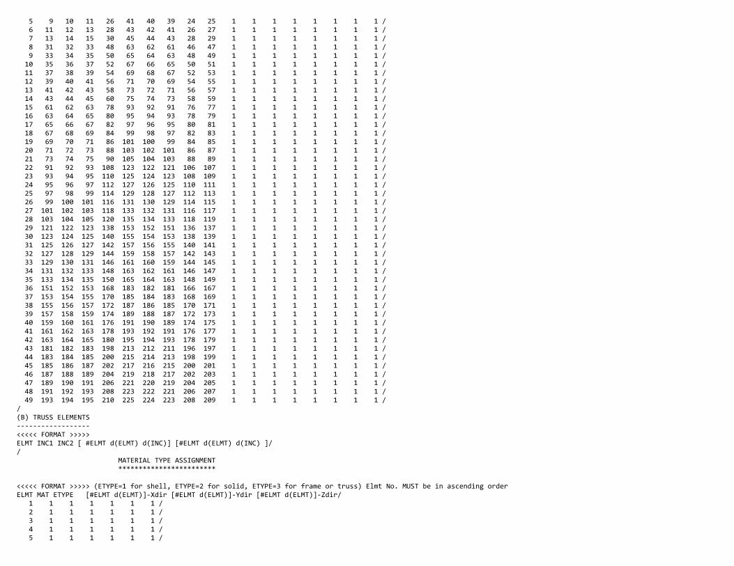
5 9 10 11 26 41 40 39 24 25 1 1 1 1 1 1 1 1 / 6 11 12 13 28 43 42 41 26 27 1 1 1 1 1 1 1 1 / 7 13 14 15 30 45 44 43 28 29 1 1 1 1 1 1 1 1 / 8 31 32 33 48 63 62 61 46 47 1 1 1 1 1 1 1 1 / 9 33 34 35 50 65 64 63 48 49 1 1 1 1 1 1 1 1 / 10 35 36 37 52 67 66 65 50 51 1 1 1 1 1 1 1 1 / 11 37 38 39 54 69 68 67 52 53 1 1 1 1 1 1 1 1 / 12 39 40 41 56 71 70 69 54 55 1 1 1 1 1 1 1 1 / 13 41 42 43 58 73 72 71 56 57 1 1 1 1 1 1 1 1 / 14 43 44 45 60 75 74 73 58 59 1 1 1 1 1 1 1 1 / 15 61 62 63 78 93 92 91 76 77 1 1 1 1 1 1 1 1 / 16 63 64 65 80 95 94 93 78 79 1 1 1 1 1 1 1 1 / 17 65 66 67 82 97 96 95 80 81 1 1 1 1 1 1 1 1 / 18 67 68 69 84 99 98 97 82 83 1 1 1 1 1 1 1 1 / 19 69 70 71 86 101 100 99 84 85 1 1 1 1 1 1 1 1 / 20 71 72 73 88 103 102 101 86 87 1 1 1 1 1 1 1 1 / 21 73 74 75 90 105 104 103 88 89 1 1 1 1 1 1 1 1 / 22 91 92 93 108 123 122 121 106 107 1 1 1 1 1 1 1 1 / 23 93 94 95 110 125 124 123 108 109 1 1 1 1 1 1 1 1 / 24 95 96 97 112 127 126 125 110 111 1 1 1 1 1 1 1 1 / 25 97 98 99 114 129 128 127 112 113 1 1 1 1 1 1 1 1 / 26 99 100 101 116 131 130 129 114 115 1 1 1 1 1 1 1 1 / 27 101 102 103 118 133 132 131 116 117 1 1 1 1 1 1 1 1 / 28 103 104 105 120 135 134 133 118 119 1 1 1 1 1 1 1 1 / 29 121 122 123 138 153 152 151 136 137 1 1 1 1 1 1 1 1 / 30 123 124 125 140 155 154 153 138 139 1 1 1 1 1 1 1 1 / 31 125 126 127 142 157 156 155 140 141 1 1 1 1 1 1 1 1 / 32 127 128 129 144 159 158 157 142 143 1 1 1 1 1 1 1 1 / 33 129 130 131 146 161 160 159 144 145 1 1 1 1 1 1 1 1 / 34 131 132 133 148 163 162 161 146 147 1 1 1 1 1 1 1 1 / 35 133 134 135 150 165 164 163 148 149 1 1 1 1 1 1 1 1 / 36 151 152 153 168 183 182 181 166 167 1 1 1 1 1 1 1 1 / 37 153 154 155 170 185 184 183 168 169 1 1 1 1 1 1 1 1 / 38 155 156 157 172 187 186 185 170 171 1 1 1 1 1 1 1 1 / 39 157 158 159 174 189 188 187 172 173 1 1 1 1 1 1 1 1 / 40 159 160 161 176 191 190 189 174 175 1 1 1 1 1 1 1 1 / 41 161 162 163 178 193 192 191 176 177 1 1 1 1 1 1 1 1 / 42 163 164 165 180 195 194 193 178 179 1 1 1 1 1 1 1 1 / 43 181 182 183 198 213 212 211 196 197 1 1 1 1 1 1 1 1 / 44 183 184 185 200 215 214 213 198 199 1 1 1 1 1 1 1 1 / 45 185 186 187 202 217 216 215 200 201 1 1 1 1 1 1 1 1 / 46 187 188 189 204 219 218 217 202 203 1 1 1 1 1 1 1 1 / 47 189 190 191 206 221 220 219 204 205 1 1 1 1 1 1 1 1 / 48 191 192 193 208 223 222 221 206 207 1 1 1 1 1 1 1 1 / 49 193 194 195 210 225 224 223 208 209 1 1 1 1 1 1 1 1 //(B) TRUSS ELEMENTS‐‐‐‐‐‐‐‐‐‐‐‐‐‐‐‐‐‐<<<<< FORMAT >>>>>ELMT INC1 INC2 [ #ELMT d(ELMT) d(INC)] [#ELMT d(ELMT) d(INC) ]// MATERIAL TYPE ASSIGNMENT ************************
<<<<< FORMAT >>>>> (ETYPE=1 for shell, ETYPE=2 for solid, ETYPE=3 for frame or truss) Elmt No. MUST be in ascending orderELMT MAT ETYPE [#ELMT d(ELMT)]‐Xdir [#ELMT d(ELMT)]‐Ydir [#ELMT d(ELMT)]‐Zdir/ 1 1 1 1 1 1 1 / 2 1 1 1 1 1 1 / 3 1 1 1 1 1 1 / 4 1 1 1 1 1 1 / 5 1 1 1 1 1 1 /

6 1 1 1 1 1 1 / 7 1 1 1 1 1 1 / 8 1 1 1 1 1 1 / 9 1 1 1 1 1 1 / 10 1 1 1 1 1 1 / 11 1 1 1 1 1 1 / 12 1 1 1 1 1 1 / 13 1 1 1 1 1 1 / 14 1 1 1 1 1 1 / 15 1 1 1 1 1 1 / 16 1 1 1 1 1 1 / 17 1 1 1 1 1 1 / 18 1 1 1 1 1 1 / 19 1 1 1 1 1 1 / 20 1 1 1 1 1 1 / 21 1 1 1 1 1 1 / 22 1 1 1 1 1 1 / 23 1 1 1 1 1 1 / 24 1 1 1 1 1 1 / 25 1 1 1 1 1 1 / 26 1 1 1 1 1 1 / 27 1 1 1 1 1 1 / 28 1 1 1 1 1 1 / 29 1 1 1 1 1 1 / 30 1 1 1 1 1 1 / 31 1 1 1 1 1 1 / 32 1 1 1 1 1 1 / 33 1 1 1 1 1 1 / 34 1 1 1 1 1 1 / 35 1 1 1 1 1 1 / 36 1 1 1 1 1 1 / 37 1 1 1 1 1 1 / 38 1 1 1 1 1 1 / 39 1 1 1 1 1 1 / 40 1 1 1 1 1 1 / 41 1 1 1 1 1 1 / 42 1 1 1 1 1 1 / 43 1 1 1 1 1 1 / 44 1 1 1 1 1 1 / 45 1 1 1 1 1 1 / 46 1 1 1 1 1 1 / 47 1 1 1 1 1 1 / 48 1 1 1 1 1 1 / 49 1 1 1 1 1 1 // COORDINATES ***********
<<<<< FORMAT >>>>> (units = mm) <TOP or C/L> < BOT > NODE TYPE X Y Z <X Y Z> [ #NODES d(NODES) d(X) d(Y) d(Z) ] [ #NODES d(NODES) d(X) d(Y) d(Z) ]/ 1 2 0.000 0.000 0.000 1 1 0.000 0.000 0.000 1 1 0.000 0.000 0.000 1 1 0.000 0.000 0.000 / 2 2 76.250 0.000 0.000 1 1 0.000 0.000 0.000 1 1 0.000 0.000 0.000 1 1 0.000 0.000 0.000 / 3 2 152.500 0.000 0.000 1 1 0.000 0.000 0.000 1 1 0.000 0.000 0.000 1 1 0.000 0.000 0.000 / 4 2 228.750 0.000 0.000 1 1 0.000 0.000 0.000 1 1 0.000 0.000 0.000 1 1 0.000 0.000 0.000 / 5 2 305.000 0.000 0.000 1 1 0.000 0.000 0.000 1 1 0.000 0.000 0.000 1 1 0.000 0.000 0.000 / 6 2 381.250 0.000 0.000 1 1 0.000 0.000 0.000 1 1 0.000 0.000 0.000 1 1 0.000 0.000 0.000 / 7 2 457.500 0.000 0.000 1 1 0.000 0.000 0.000 1 1 0.000 0.000 0.000 1 1 0.000 0.000 0.000 / 8 2 533.750 0.000 0.000 1 1 0.000 0.000 0.000 1 1 0.000 0.000 0.000 1 1 0.000 0.000 0.000 / 9 2 610.000 0.000 0.000 1 1 0.000 0.000 0.000 1 1 0.000 0.000 0.000 1 1 0.000 0.000 0.000 / 10 2 686.250 0.000 0.000 1 1 0.000 0.000 0.000 1 1 0.000 0.000 0.000 1 1 0.000 0.000 0.000 /
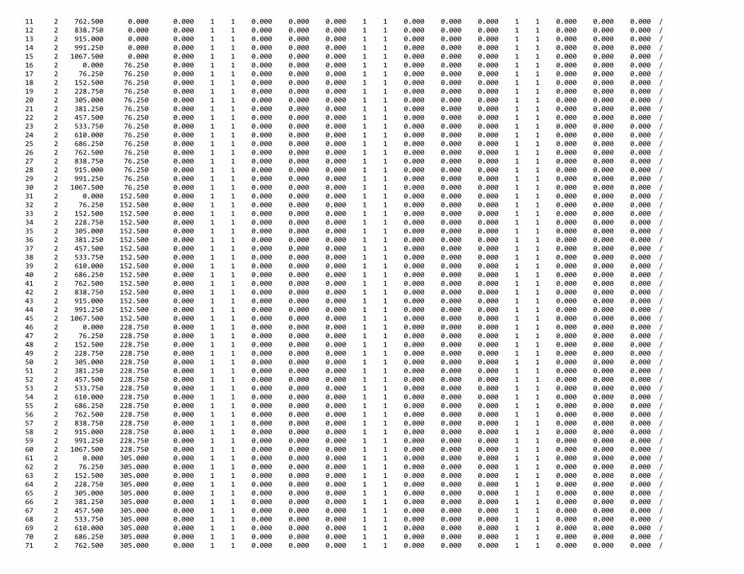
11 2 762.500 0.000 0.000 1 1 0.000 0.000 0.000 1 1 0.000 0.000 0.000 1 1 0.000 0.000 0.000 / 12 2 838.750 0.000 0.000 1 1 0.000 0.000 0.000 1 1 0.000 0.000 0.000 1 1 0.000 0.000 0.000 / 13 2 915.000 0.000 0.000 1 1 0.000 0.000 0.000 1 1 0.000 0.000 0.000 1 1 0.000 0.000 0.000 / 14 2 991.250 0.000 0.000 1 1 0.000 0.000 0.000 1 1 0.000 0.000 0.000 1 1 0.000 0.000 0.000 / 15 2 1067.500 0.000 0.000 1 1 0.000 0.000 0.000 1 1 0.000 0.000 0.000 1 1 0.000 0.000 0.000 / 16 2 0.000 76.250 0.000 1 1 0.000 0.000 0.000 1 1 0.000 0.000 0.000 1 1 0.000 0.000 0.000 / 17 2 76.250 76.250 0.000 1 1 0.000 0.000 0.000 1 1 0.000 0.000 0.000 1 1 0.000 0.000 0.000 / 18 2 152.500 76.250 0.000 1 1 0.000 0.000 0.000 1 1 0.000 0.000 0.000 1 1 0.000 0.000 0.000 / 19 2 228.750 76.250 0.000 1 1 0.000 0.000 0.000 1 1 0.000 0.000 0.000 1 1 0.000 0.000 0.000 / 20 2 305.000 76.250 0.000 1 1 0.000 0.000 0.000 1 1 0.000 0.000 0.000 1 1 0.000 0.000 0.000 / 21 2 381.250 76.250 0.000 1 1 0.000 0.000 0.000 1 1 0.000 0.000 0.000 1 1 0.000 0.000 0.000 / 22 2 457.500 76.250 0.000 1 1 0.000 0.000 0.000 1 1 0.000 0.000 0.000 1 1 0.000 0.000 0.000 / 23 2 533.750 76.250 0.000 1 1 0.000 0.000 0.000 1 1 0.000 0.000 0.000 1 1 0.000 0.000 0.000 / 24 2 610.000 76.250 0.000 1 1 0.000 0.000 0.000 1 1 0.000 0.000 0.000 1 1 0.000 0.000 0.000 / 25 2 686.250 76.250 0.000 1 1 0.000 0.000 0.000 1 1 0.000 0.000 0.000 1 1 0.000 0.000 0.000 / 26 2 762.500 76.250 0.000 1 1 0.000 0.000 0.000 1 1 0.000 0.000 0.000 1 1 0.000 0.000 0.000 / 27 2 838.750 76.250 0.000 1 1 0.000 0.000 0.000 1 1 0.000 0.000 0.000 1 1 0.000 0.000 0.000 / 28 2 915.000 76.250 0.000 1 1 0.000 0.000 0.000 1 1 0.000 0.000 0.000 1 1 0.000 0.000 0.000 / 29 2 991.250 76.250 0.000 1 1 0.000 0.000 0.000 1 1 0.000 0.000 0.000 1 1 0.000 0.000 0.000 / 30 2 1067.500 76.250 0.000 1 1 0.000 0.000 0.000 1 1 0.000 0.000 0.000 1 1 0.000 0.000 0.000 / 31 2 0.000 152.500 0.000 1 1 0.000 0.000 0.000 1 1 0.000 0.000 0.000 1 1 0.000 0.000 0.000 / 32 2 76.250 152.500 0.000 1 1 0.000 0.000 0.000 1 1 0.000 0.000 0.000 1 1 0.000 0.000 0.000 / 33 2 152.500 152.500 0.000 1 1 0.000 0.000 0.000 1 1 0.000 0.000 0.000 1 1 0.000 0.000 0.000 / 34 2 228.750 152.500 0.000 1 1 0.000 0.000 0.000 1 1 0.000 0.000 0.000 1 1 0.000 0.000 0.000 / 35 2 305.000 152.500 0.000 1 1 0.000 0.000 0.000 1 1 0.000 0.000 0.000 1 1 0.000 0.000 0.000 / 36 2 381.250 152.500 0.000 1 1 0.000 0.000 0.000 1 1 0.000 0.000 0.000 1 1 0.000 0.000 0.000 / 37 2 457.500 152.500 0.000 1 1 0.000 0.000 0.000 1 1 0.000 0.000 0.000 1 1 0.000 0.000 0.000 / 38 2 533.750 152.500 0.000 1 1 0.000 0.000 0.000 1 1 0.000 0.000 0.000 1 1 0.000 0.000 0.000 / 39 2 610.000 152.500 0.000 1 1 0.000 0.000 0.000 1 1 0.000 0.000 0.000 1 1 0.000 0.000 0.000 / 40 2 686.250 152.500 0.000 1 1 0.000 0.000 0.000 1 1 0.000 0.000 0.000 1 1 0.000 0.000 0.000 / 41 2 762.500 152.500 0.000 1 1 0.000 0.000 0.000 1 1 0.000 0.000 0.000 1 1 0.000 0.000 0.000 / 42 2 838.750 152.500 0.000 1 1 0.000 0.000 0.000 1 1 0.000 0.000 0.000 1 1 0.000 0.000 0.000 / 43 2 915.000 152.500 0.000 1 1 0.000 0.000 0.000 1 1 0.000 0.000 0.000 1 1 0.000 0.000 0.000 / 44 2 991.250 152.500 0.000 1 1 0.000 0.000 0.000 1 1 0.000 0.000 0.000 1 1 0.000 0.000 0.000 / 45 2 1067.500 152.500 0.000 1 1 0.000 0.000 0.000 1 1 0.000 0.000 0.000 1 1 0.000 0.000 0.000 / 46 2 0.000 228.750 0.000 1 1 0.000 0.000 0.000 1 1 0.000 0.000 0.000 1 1 0.000 0.000 0.000 / 47 2 76.250 228.750 0.000 1 1 0.000 0.000 0.000 1 1 0.000 0.000 0.000 1 1 0.000 0.000 0.000 / 48 2 152.500 228.750 0.000 1 1 0.000 0.000 0.000 1 1 0.000 0.000 0.000 1 1 0.000 0.000 0.000 / 49 2 228.750 228.750 0.000 1 1 0.000 0.000 0.000 1 1 0.000 0.000 0.000 1 1 0.000 0.000 0.000 / 50 2 305.000 228.750 0.000 1 1 0.000 0.000 0.000 1 1 0.000 0.000 0.000 1 1 0.000 0.000 0.000 / 51 2 381.250 228.750 0.000 1 1 0.000 0.000 0.000 1 1 0.000 0.000 0.000 1 1 0.000 0.000 0.000 / 52 2 457.500 228.750 0.000 1 1 0.000 0.000 0.000 1 1 0.000 0.000 0.000 1 1 0.000 0.000 0.000 / 53 2 533.750 228.750 0.000 1 1 0.000 0.000 0.000 1 1 0.000 0.000 0.000 1 1 0.000 0.000 0.000 / 54 2 610.000 228.750 0.000 1 1 0.000 0.000 0.000 1 1 0.000 0.000 0.000 1 1 0.000 0.000 0.000 / 55 2 686.250 228.750 0.000 1 1 0.000 0.000 0.000 1 1 0.000 0.000 0.000 1 1 0.000 0.000 0.000 / 56 2 762.500 228.750 0.000 1 1 0.000 0.000 0.000 1 1 0.000 0.000 0.000 1 1 0.000 0.000 0.000 / 57 2 838.750 228.750 0.000 1 1 0.000 0.000 0.000 1 1 0.000 0.000 0.000 1 1 0.000 0.000 0.000 / 58 2 915.000 228.750 0.000 1 1 0.000 0.000 0.000 1 1 0.000 0.000 0.000 1 1 0.000 0.000 0.000 / 59 2 991.250 228.750 0.000 1 1 0.000 0.000 0.000 1 1 0.000 0.000 0.000 1 1 0.000 0.000 0.000 / 60 2 1067.500 228.750 0.000 1 1 0.000 0.000 0.000 1 1 0.000 0.000 0.000 1 1 0.000 0.000 0.000 / 61 2 0.000 305.000 0.000 1 1 0.000 0.000 0.000 1 1 0.000 0.000 0.000 1 1 0.000 0.000 0.000 / 62 2 76.250 305.000 0.000 1 1 0.000 0.000 0.000 1 1 0.000 0.000 0.000 1 1 0.000 0.000 0.000 / 63 2 152.500 305.000 0.000 1 1 0.000 0.000 0.000 1 1 0.000 0.000 0.000 1 1 0.000 0.000 0.000 / 64 2 228.750 305.000 0.000 1 1 0.000 0.000 0.000 1 1 0.000 0.000 0.000 1 1 0.000 0.000 0.000 / 65 2 305.000 305.000 0.000 1 1 0.000 0.000 0.000 1 1 0.000 0.000 0.000 1 1 0.000 0.000 0.000 / 66 2 381.250 305.000 0.000 1 1 0.000 0.000 0.000 1 1 0.000 0.000 0.000 1 1 0.000 0.000 0.000 / 67 2 457.500 305.000 0.000 1 1 0.000 0.000 0.000 1 1 0.000 0.000 0.000 1 1 0.000 0.000 0.000 / 68 2 533.750 305.000 0.000 1 1 0.000 0.000 0.000 1 1 0.000 0.000 0.000 1 1 0.000 0.000 0.000 / 69 2 610.000 305.000 0.000 1 1 0.000 0.000 0.000 1 1 0.000 0.000 0.000 1 1 0.000 0.000 0.000 / 70 2 686.250 305.000 0.000 1 1 0.000 0.000 0.000 1 1 0.000 0.000 0.000 1 1 0.000 0.000 0.000 / 71 2 762.500 305.000 0.000 1 1 0.000 0.000 0.000 1 1 0.000 0.000 0.000 1 1 0.000 0.000 0.000 /

72 2 838.750 305.000 0.000 1 1 0.000 0.000 0.000 1 1 0.000 0.000 0.000 1 1 0.000 0.000 0.000 / 73 2 915.000 305.000 0.000 1 1 0.000 0.000 0.000 1 1 0.000 0.000 0.000 1 1 0.000 0.000 0.000 / 74 2 991.250 305.000 0.000 1 1 0.000 0.000 0.000 1 1 0.000 0.000 0.000 1 1 0.000 0.000 0.000 / 75 2 1067.500 305.000 0.000 1 1 0.000 0.000 0.000 1 1 0.000 0.000 0.000 1 1 0.000 0.000 0.000 / 76 2 0.000 381.250 0.000 1 1 0.000 0.000 0.000 1 1 0.000 0.000 0.000 1 1 0.000 0.000 0.000 / 77 2 76.250 381.250 0.000 1 1 0.000 0.000 0.000 1 1 0.000 0.000 0.000 1 1 0.000 0.000 0.000 / 78 2 152.500 381.250 0.000 1 1 0.000 0.000 0.000 1 1 0.000 0.000 0.000 1 1 0.000 0.000 0.000 / 79 2 228.750 381.250 0.000 1 1 0.000 0.000 0.000 1 1 0.000 0.000 0.000 1 1 0.000 0.000 0.000 / 80 2 305.000 381.250 0.000 1 1 0.000 0.000 0.000 1 1 0.000 0.000 0.000 1 1 0.000 0.000 0.000 / 81 2 381.250 381.250 0.000 1 1 0.000 0.000 0.000 1 1 0.000 0.000 0.000 1 1 0.000 0.000 0.000 / 82 2 457.500 381.250 0.000 1 1 0.000 0.000 0.000 1 1 0.000 0.000 0.000 1 1 0.000 0.000 0.000 / 83 2 533.750 381.250 0.000 1 1 0.000 0.000 0.000 1 1 0.000 0.000 0.000 1 1 0.000 0.000 0.000 / 84 2 610.000 381.250 0.000 1 1 0.000 0.000 0.000 1 1 0.000 0.000 0.000 1 1 0.000 0.000 0.000 / 85 2 686.250 381.250 0.000 1 1 0.000 0.000 0.000 1 1 0.000 0.000 0.000 1 1 0.000 0.000 0.000 / 86 2 762.500 381.250 0.000 1 1 0.000 0.000 0.000 1 1 0.000 0.000 0.000 1 1 0.000 0.000 0.000 / 87 2 838.750 381.250 0.000 1 1 0.000 0.000 0.000 1 1 0.000 0.000 0.000 1 1 0.000 0.000 0.000 / 88 2 915.000 381.250 0.000 1 1 0.000 0.000 0.000 1 1 0.000 0.000 0.000 1 1 0.000 0.000 0.000 / 89 2 991.250 381.250 0.000 1 1 0.000 0.000 0.000 1 1 0.000 0.000 0.000 1 1 0.000 0.000 0.000 / 90 2 1067.500 381.250 0.000 1 1 0.000 0.000 0.000 1 1 0.000 0.000 0.000 1 1 0.000 0.000 0.000 / 91 2 0.000 457.500 0.000 1 1 0.000 0.000 0.000 1 1 0.000 0.000 0.000 1 1 0.000 0.000 0.000 / 92 2 76.250 457.500 0.000 1 1 0.000 0.000 0.000 1 1 0.000 0.000 0.000 1 1 0.000 0.000 0.000 / 93 2 152.500 457.500 0.000 1 1 0.000 0.000 0.000 1 1 0.000 0.000 0.000 1 1 0.000 0.000 0.000 / 94 2 228.750 457.500 0.000 1 1 0.000 0.000 0.000 1 1 0.000 0.000 0.000 1 1 0.000 0.000 0.000 / 95 2 305.000 457.500 0.000 1 1 0.000 0.000 0.000 1 1 0.000 0.000 0.000 1 1 0.000 0.000 0.000 / 96 2 381.250 457.500 0.000 1 1 0.000 0.000 0.000 1 1 0.000 0.000 0.000 1 1 0.000 0.000 0.000 / 97 2 457.500 457.500 0.000 1 1 0.000 0.000 0.000 1 1 0.000 0.000 0.000 1 1 0.000 0.000 0.000 / 98 2 533.750 457.500 0.000 1 1 0.000 0.000 0.000 1 1 0.000 0.000 0.000 1 1 0.000 0.000 0.000 / 99 2 610.000 457.500 0.000 1 1 0.000 0.000 0.000 1 1 0.000 0.000 0.000 1 1 0.000 0.000 0.000 / 100 2 686.250 457.500 0.000 1 1 0.000 0.000 0.000 1 1 0.000 0.000 0.000 1 1 0.000 0.000 0.000 / 101 2 762.500 457.500 0.000 1 1 0.000 0.000 0.000 1 1 0.000 0.000 0.000 1 1 0.000 0.000 0.000 / 102 2 838.750 457.500 0.000 1 1 0.000 0.000 0.000 1 1 0.000 0.000 0.000 1 1 0.000 0.000 0.000 / 103 2 915.000 457.500 0.000 1 1 0.000 0.000 0.000 1 1 0.000 0.000 0.000 1 1 0.000 0.000 0.000 / 104 2 991.250 457.500 0.000 1 1 0.000 0.000 0.000 1 1 0.000 0.000 0.000 1 1 0.000 0.000 0.000 / 105 2 1067.500 457.500 0.000 1 1 0.000 0.000 0.000 1 1 0.000 0.000 0.000 1 1 0.000 0.000 0.000 / 106 2 0.000 533.750 0.000 1 1 0.000 0.000 0.000 1 1 0.000 0.000 0.000 1 1 0.000 0.000 0.000 / 107 2 76.250 533.750 0.000 1 1 0.000 0.000 0.000 1 1 0.000 0.000 0.000 1 1 0.000 0.000 0.000 / 108 2 152.500 533.750 0.000 1 1 0.000 0.000 0.000 1 1 0.000 0.000 0.000 1 1 0.000 0.000 0.000 / 109 2 228.750 533.750 0.000 1 1 0.000 0.000 0.000 1 1 0.000 0.000 0.000 1 1 0.000 0.000 0.000 / 110 2 305.000 533.750 0.000 1 1 0.000 0.000 0.000 1 1 0.000 0.000 0.000 1 1 0.000 0.000 0.000 / 111 2 381.250 533.750 0.000 1 1 0.000 0.000 0.000 1 1 0.000 0.000 0.000 1 1 0.000 0.000 0.000 / 112 2 457.500 533.750 0.000 1 1 0.000 0.000 0.000 1 1 0.000 0.000 0.000 1 1 0.000 0.000 0.000 / 113 2 533.750 533.750 0.000 1 1 0.000 0.000 0.000 1 1 0.000 0.000 0.000 1 1 0.000 0.000 0.000 / 114 2 610.000 533.750 0.000 1 1 0.000 0.000 0.000 1 1 0.000 0.000 0.000 1 1 0.000 0.000 0.000 / 115 2 686.250 533.750 0.000 1 1 0.000 0.000 0.000 1 1 0.000 0.000 0.000 1 1 0.000 0.000 0.000 / 116 2 762.500 533.750 0.000 1 1 0.000 0.000 0.000 1 1 0.000 0.000 0.000 1 1 0.000 0.000 0.000 / 117 2 838.750 533.750 0.000 1 1 0.000 0.000 0.000 1 1 0.000 0.000 0.000 1 1 0.000 0.000 0.000 / 118 2 915.000 533.750 0.000 1 1 0.000 0.000 0.000 1 1 0.000 0.000 0.000 1 1 0.000 0.000 0.000 / 119 2 991.250 533.750 0.000 1 1 0.000 0.000 0.000 1 1 0.000 0.000 0.000 1 1 0.000 0.000 0.000 / 120 2 1067.500 533.750 0.000 1 1 0.000 0.000 0.000 1 1 0.000 0.000 0.000 1 1 0.000 0.000 0.000 / 121 2 0.000 610.000 0.000 1 1 0.000 0.000 0.000 1 1 0.000 0.000 0.000 1 1 0.000 0.000 0.000 / 122 2 76.250 610.000 0.000 1 1 0.000 0.000 0.000 1 1 0.000 0.000 0.000 1 1 0.000 0.000 0.000 / 123 2 152.500 610.000 0.000 1 1 0.000 0.000 0.000 1 1 0.000 0.000 0.000 1 1 0.000 0.000 0.000 / 124 2 228.750 610.000 0.000 1 1 0.000 0.000 0.000 1 1 0.000 0.000 0.000 1 1 0.000 0.000 0.000 / 125 2 305.000 610.000 0.000 1 1 0.000 0.000 0.000 1 1 0.000 0.000 0.000 1 1 0.000 0.000 0.000 / 126 2 381.250 610.000 0.000 1 1 0.000 0.000 0.000 1 1 0.000 0.000 0.000 1 1 0.000 0.000 0.000 / 127 2 457.500 610.000 0.000 1 1 0.000 0.000 0.000 1 1 0.000 0.000 0.000 1 1 0.000 0.000 0.000 / 128 2 533.750 610.000 0.000 1 1 0.000 0.000 0.000 1 1 0.000 0.000 0.000 1 1 0.000 0.000 0.000 / 129 2 610.000 610.000 0.000 1 1 0.000 0.000 0.000 1 1 0.000 0.000 0.000 1 1 0.000 0.000 0.000 / 130 2 686.250 610.000 0.000 1 1 0.000 0.000 0.000 1 1 0.000 0.000 0.000 1 1 0.000 0.000 0.000 / 131 2 762.500 610.000 0.000 1 1 0.000 0.000 0.000 1 1 0.000 0.000 0.000 1 1 0.000 0.000 0.000 / 132 2 838.750 610.000 0.000 1 1 0.000 0.000 0.000 1 1 0.000 0.000 0.000 1 1 0.000 0.000 0.000 /

133 2 915.000 610.000 0.000 1 1 0.000 0.000 0.000 1 1 0.000 0.000 0.000 1 1 0.000 0.000 0.000 / 134 2 991.250 610.000 0.000 1 1 0.000 0.000 0.000 1 1 0.000 0.000 0.000 1 1 0.000 0.000 0.000 / 135 2 1067.500 610.000 0.000 1 1 0.000 0.000 0.000 1 1 0.000 0.000 0.000 1 1 0.000 0.000 0.000 / 136 2 0.000 686.250 0.000 1 1 0.000 0.000 0.000 1 1 0.000 0.000 0.000 1 1 0.000 0.000 0.000 / 137 2 76.250 686.250 0.000 1 1 0.000 0.000 0.000 1 1 0.000 0.000 0.000 1 1 0.000 0.000 0.000 / 138 2 152.500 686.250 0.000 1 1 0.000 0.000 0.000 1 1 0.000 0.000 0.000 1 1 0.000 0.000 0.000 / 139 2 228.750 686.250 0.000 1 1 0.000 0.000 0.000 1 1 0.000 0.000 0.000 1 1 0.000 0.000 0.000 / 140 2 305.000 686.250 0.000 1 1 0.000 0.000 0.000 1 1 0.000 0.000 0.000 1 1 0.000 0.000 0.000 / 141 2 381.250 686.250 0.000 1 1 0.000 0.000 0.000 1 1 0.000 0.000 0.000 1 1 0.000 0.000 0.000 / 142 2 457.500 686.250 0.000 1 1 0.000 0.000 0.000 1 1 0.000 0.000 0.000 1 1 0.000 0.000 0.000 / 143 2 533.750 686.250 0.000 1 1 0.000 0.000 0.000 1 1 0.000 0.000 0.000 1 1 0.000 0.000 0.000 / 144 2 610.000 686.250 0.000 1 1 0.000 0.000 0.000 1 1 0.000 0.000 0.000 1 1 0.000 0.000 0.000 / 145 2 686.250 686.250 0.000 1 1 0.000 0.000 0.000 1 1 0.000 0.000 0.000 1 1 0.000 0.000 0.000 / 146 2 762.500 686.250 0.000 1 1 0.000 0.000 0.000 1 1 0.000 0.000 0.000 1 1 0.000 0.000 0.000 / 147 2 838.750 686.250 0.000 1 1 0.000 0.000 0.000 1 1 0.000 0.000 0.000 1 1 0.000 0.000 0.000 / 148 2 915.000 686.250 0.000 1 1 0.000 0.000 0.000 1 1 0.000 0.000 0.000 1 1 0.000 0.000 0.000 / 149 2 991.250 686.250 0.000 1 1 0.000 0.000 0.000 1 1 0.000 0.000 0.000 1 1 0.000 0.000 0.000 / 150 2 1067.500 686.250 0.000 1 1 0.000 0.000 0.000 1 1 0.000 0.000 0.000 1 1 0.000 0.000 0.000 / 151 2 0.000 762.500 0.000 1 1 0.000 0.000 0.000 1 1 0.000 0.000 0.000 1 1 0.000 0.000 0.000 / 152 2 76.250 762.500 0.000 1 1 0.000 0.000 0.000 1 1 0.000 0.000 0.000 1 1 0.000 0.000 0.000 / 153 2 152.500 762.500 0.000 1 1 0.000 0.000 0.000 1 1 0.000 0.000 0.000 1 1 0.000 0.000 0.000 / 154 2 228.750 762.500 0.000 1 1 0.000 0.000 0.000 1 1 0.000 0.000 0.000 1 1 0.000 0.000 0.000 / 155 2 305.000 762.500 0.000 1 1 0.000 0.000 0.000 1 1 0.000 0.000 0.000 1 1 0.000 0.000 0.000 / 156 2 381.250 762.500 0.000 1 1 0.000 0.000 0.000 1 1 0.000 0.000 0.000 1 1 0.000 0.000 0.000 / 157 2 457.500 762.500 0.000 1 1 0.000 0.000 0.000 1 1 0.000 0.000 0.000 1 1 0.000 0.000 0.000 / 158 2 533.750 762.500 0.000 1 1 0.000 0.000 0.000 1 1 0.000 0.000 0.000 1 1 0.000 0.000 0.000 / 159 2 610.000 762.500 0.000 1 1 0.000 0.000 0.000 1 1 0.000 0.000 0.000 1 1 0.000 0.000 0.000 / 160 2 686.250 762.500 0.000 1 1 0.000 0.000 0.000 1 1 0.000 0.000 0.000 1 1 0.000 0.000 0.000 / 161 2 762.500 762.500 0.000 1 1 0.000 0.000 0.000 1 1 0.000 0.000 0.000 1 1 0.000 0.000 0.000 / 162 2 838.750 762.500 0.000 1 1 0.000 0.000 0.000 1 1 0.000 0.000 0.000 1 1 0.000 0.000 0.000 / 163 2 915.000 762.500 0.000 1 1 0.000 0.000 0.000 1 1 0.000 0.000 0.000 1 1 0.000 0.000 0.000 / 164 2 991.250 762.500 0.000 1 1 0.000 0.000 0.000 1 1 0.000 0.000 0.000 1 1 0.000 0.000 0.000 / 165 2 1067.500 762.500 0.000 1 1 0.000 0.000 0.000 1 1 0.000 0.000 0.000 1 1 0.000 0.000 0.000 / 166 2 0.000 838.750 0.000 1 1 0.000 0.000 0.000 1 1 0.000 0.000 0.000 1 1 0.000 0.000 0.000 / 167 2 76.250 838.750 0.000 1 1 0.000 0.000 0.000 1 1 0.000 0.000 0.000 1 1 0.000 0.000 0.000 / 168 2 152.500 838.750 0.000 1 1 0.000 0.000 0.000 1 1 0.000 0.000 0.000 1 1 0.000 0.000 0.000 / 169 2 228.750 838.750 0.000 1 1 0.000 0.000 0.000 1 1 0.000 0.000 0.000 1 1 0.000 0.000 0.000 / 170 2 305.000 838.750 0.000 1 1 0.000 0.000 0.000 1 1 0.000 0.000 0.000 1 1 0.000 0.000 0.000 / 171 2 381.250 838.750 0.000 1 1 0.000 0.000 0.000 1 1 0.000 0.000 0.000 1 1 0.000 0.000 0.000 / 172 2 457.500 838.750 0.000 1 1 0.000 0.000 0.000 1 1 0.000 0.000 0.000 1 1 0.000 0.000 0.000 / 173 2 533.750 838.750 0.000 1 1 0.000 0.000 0.000 1 1 0.000 0.000 0.000 1 1 0.000 0.000 0.000 / 174 2 610.000 838.750 0.000 1 1 0.000 0.000 0.000 1 1 0.000 0.000 0.000 1 1 0.000 0.000 0.000 / 175 2 686.250 838.750 0.000 1 1 0.000 0.000 0.000 1 1 0.000 0.000 0.000 1 1 0.000 0.000 0.000 / 176 2 762.500 838.750 0.000 1 1 0.000 0.000 0.000 1 1 0.000 0.000 0.000 1 1 0.000 0.000 0.000 / 177 2 838.750 838.750 0.000 1 1 0.000 0.000 0.000 1 1 0.000 0.000 0.000 1 1 0.000 0.000 0.000 / 178 2 915.000 838.750 0.000 1 1 0.000 0.000 0.000 1 1 0.000 0.000 0.000 1 1 0.000 0.000 0.000 / 179 2 991.250 838.750 0.000 1 1 0.000 0.000 0.000 1 1 0.000 0.000 0.000 1 1 0.000 0.000 0.000 / 180 2 1067.500 838.750 0.000 1 1 0.000 0.000 0.000 1 1 0.000 0.000 0.000 1 1 0.000 0.000 0.000 / 181 2 0.000 915.000 0.000 1 1 0.000 0.000 0.000 1 1 0.000 0.000 0.000 1 1 0.000 0.000 0.000 / 182 2 76.250 915.000 0.000 1 1 0.000 0.000 0.000 1 1 0.000 0.000 0.000 1 1 0.000 0.000 0.000 / 183 2 152.500 915.000 0.000 1 1 0.000 0.000 0.000 1 1 0.000 0.000 0.000 1 1 0.000 0.000 0.000 / 184 2 228.750 915.000 0.000 1 1 0.000 0.000 0.000 1 1 0.000 0.000 0.000 1 1 0.000 0.000 0.000 / 185 2 305.000 915.000 0.000 1 1 0.000 0.000 0.000 1 1 0.000 0.000 0.000 1 1 0.000 0.000 0.000 / 186 2 381.250 915.000 0.000 1 1 0.000 0.000 0.000 1 1 0.000 0.000 0.000 1 1 0.000 0.000 0.000 / 187 2 457.500 915.000 0.000 1 1 0.000 0.000 0.000 1 1 0.000 0.000 0.000 1 1 0.000 0.000 0.000 / 188 2 533.750 915.000 0.000 1 1 0.000 0.000 0.000 1 1 0.000 0.000 0.000 1 1 0.000 0.000 0.000 / 189 2 610.000 915.000 0.000 1 1 0.000 0.000 0.000 1 1 0.000 0.000 0.000 1 1 0.000 0.000 0.000 / 190 2 686.250 915.000 0.000 1 1 0.000 0.000 0.000 1 1 0.000 0.000 0.000 1 1 0.000 0.000 0.000 / 191 2 762.500 915.000 0.000 1 1 0.000 0.000 0.000 1 1 0.000 0.000 0.000 1 1 0.000 0.000 0.000 / 192 2 838.750 915.000 0.000 1 1 0.000 0.000 0.000 1 1 0.000 0.000 0.000 1 1 0.000 0.000 0.000 / 193 2 915.000 915.000 0.000 1 1 0.000 0.000 0.000 1 1 0.000 0.000 0.000 1 1 0.000 0.000 0.000 /

194 2 991.250 915.000 0.000 1 1 0.000 0.000 0.000 1 1 0.000 0.000 0.000 1 1 0.000 0.000 0.000 / 195 2 1067.500 915.000 0.000 1 1 0.000 0.000 0.000 1 1 0.000 0.000 0.000 1 1 0.000 0.000 0.000 / 196 2 0.000 991.250 0.000 1 1 0.000 0.000 0.000 1 1 0.000 0.000 0.000 1 1 0.000 0.000 0.000 / 197 2 76.250 991.250 0.000 1 1 0.000 0.000 0.000 1 1 0.000 0.000 0.000 1 1 0.000 0.000 0.000 / 198 2 152.500 991.250 0.000 1 1 0.000 0.000 0.000 1 1 0.000 0.000 0.000 1 1 0.000 0.000 0.000 / 199 2 228.750 991.250 0.000 1 1 0.000 0.000 0.000 1 1 0.000 0.000 0.000 1 1 0.000 0.000 0.000 / 200 2 305.000 991.250 0.000 1 1 0.000 0.000 0.000 1 1 0.000 0.000 0.000 1 1 0.000 0.000 0.000 / 201 2 381.250 991.250 0.000 1 1 0.000 0.000 0.000 1 1 0.000 0.000 0.000 1 1 0.000 0.000 0.000 / 202 2 457.500 991.250 0.000 1 1 0.000 0.000 0.000 1 1 0.000 0.000 0.000 1 1 0.000 0.000 0.000 / 203 2 533.750 991.250 0.000 1 1 0.000 0.000 0.000 1 1 0.000 0.000 0.000 1 1 0.000 0.000 0.000 / 204 2 610.000 991.250 0.000 1 1 0.000 0.000 0.000 1 1 0.000 0.000 0.000 1 1 0.000 0.000 0.000 / 205 2 686.250 991.250 0.000 1 1 0.000 0.000 0.000 1 1 0.000 0.000 0.000 1 1 0.000 0.000 0.000 / 206 2 762.500 991.250 0.000 1 1 0.000 0.000 0.000 1 1 0.000 0.000 0.000 1 1 0.000 0.000 0.000 / 207 2 838.750 991.250 0.000 1 1 0.000 0.000 0.000 1 1 0.000 0.000 0.000 1 1 0.000 0.000 0.000 / 208 2 915.000 991.250 0.000 1 1 0.000 0.000 0.000 1 1 0.000 0.000 0.000 1 1 0.000 0.000 0.000 / 209 2 991.250 991.250 0.000 1 1 0.000 0.000 0.000 1 1 0.000 0.000 0.000 1 1 0.000 0.000 0.000 / 210 2 1067.500 991.250 0.000 1 1 0.000 0.000 0.000 1 1 0.000 0.000 0.000 1 1 0.000 0.000 0.000 / 211 2 0.000 1067.500 0.000 1 1 0.000 0.000 0.000 1 1 0.000 0.000 0.000 1 1 0.000 0.000 0.000 / 212 2 76.250 1067.500 0.000 1 1 0.000 0.000 0.000 1 1 0.000 0.000 0.000 1 1 0.000 0.000 0.000 / 213 2 152.500 1067.500 0.000 1 1 0.000 0.000 0.000 1 1 0.000 0.000 0.000 1 1 0.000 0.000 0.000 / 214 2 228.750 1067.500 0.000 1 1 0.000 0.000 0.000 1 1 0.000 0.000 0.000 1 1 0.000 0.000 0.000 / 215 2 305.000 1067.500 0.000 1 1 0.000 0.000 0.000 1 1 0.000 0.000 0.000 1 1 0.000 0.000 0.000 / 216 2 381.250 1067.500 0.000 1 1 0.000 0.000 0.000 1 1 0.000 0.000 0.000 1 1 0.000 0.000 0.000 / 217 2 457.500 1067.500 0.000 1 1 0.000 0.000 0.000 1 1 0.000 0.000 0.000 1 1 0.000 0.000 0.000 / 218 2 533.750 1067.500 0.000 1 1 0.000 0.000 0.000 1 1 0.000 0.000 0.000 1 1 0.000 0.000 0.000 / 219 2 610.000 1067.500 0.000 1 1 0.000 0.000 0.000 1 1 0.000 0.000 0.000 1 1 0.000 0.000 0.000 / 220 2 686.250 1067.500 0.000 1 1 0.000 0.000 0.000 1 1 0.000 0.000 0.000 1 1 0.000 0.000 0.000 / 221 2 762.500 1067.500 0.000 1 1 0.000 0.000 0.000 1 1 0.000 0.000 0.000 1 1 0.000 0.000 0.000 / 222 2 838.750 1067.500 0.000 1 1 0.000 0.000 0.000 1 1 0.000 0.000 0.000 1 1 0.000 0.000 0.000 / 223 2 915.000 1067.500 0.000 1 1 0.000 0.000 0.000 1 1 0.000 0.000 0.000 1 1 0.000 0.000 0.000 / 224 2 991.250 1067.500 0.000 1 1 0.000 0.000 0.000 1 1 0.000 0.000 0.000 1 1 0.000 0.000 0.000 / 225 2 1067.500 1067.500 0.000 1 1 0.000 0.000 0.000 1 1 0.000 0.000 0.000 1 1 0.000 0.000 0.000 // NODAL RESTRAINTS AND PRESCRIBED D.O.F. **************************************
<<<<< FORMAT >>>>> (units = mm, degrees)(d(NODE)>0!!!) Node No. MUST be in ascending order. Cannot repeat nodes.NODE DX‐R DY‐R DZ‐R R1‐R R2‐R [#NODES d(NODE)] [#NODES d(NODE)] [#NODES d(NODE)] / 15 1 0 0 1 0 1 1/ 30 1 0 0 1 0 1 1/ 33 0 0 1 0 0 1 1/ 39 0 0 1 0 0 1 1/ 45 1 0 1 1 0 1 1/ 60 1 0 0 1 0 1 1/ 75 1 0 0 1 0 1 1/ 90 1 0 0 1 0 1 1/ 105 1 0 0 1 0 1 1/ 120 1 0 0 1 0 1 1/ 123 0 0 1 0 0 1 1/ 135 1 0 0 1 0 1 1/ 150 1 0 0 1 0 1 1/ 165 1 0 0 1 0 1 1/ 180 1 0 0 1 0 1 1/ 195 1 0 0 1 0 1 1/ 210 1 0 0 1 0 1 1/ 211 0 1 0 0 1 1 1/ 212 0 1 0 0 1 1 1/ 213 0 1 1 0 1 1 1/ 214 0 1 0 0 1 1 1/ 215 0 1 0 0 1 1 1/ 216 0 1 0 0 1 1 1/
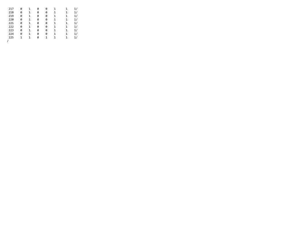
217 0 1 0 0 1 1 1/ 218 0 1 0 0 1 1 1/ 219 0 1 0 0 1 1 1/ 220 0 1 0 0 1 1 1/ 221 0 1 0 0 1 1 1/ 222 0 1 0 0 1 1 1/ 223 0 1 0 0 1 1 1/ 224 0 1 0 0 1 1 1/ 225 1 1 0 1 1 1 1//

* * * * * * * * * * * * * * L O A D C A S E * * D A T A * * Version 1.0 * * * * * * * * * * * * * *
LOAD CASE PARAMETERS ********************
Structure Title (30 char. max.) : Enter Structure TitleLoad Case Title (30 char. max.) : In‐Plane LoadingLoad Case File Name (8 char. max.) : AXIAL
No. of Elements with a u.d.l. : 0No. of Elements with Hydrostatic Loads : 0No. of Elements with Temperature Loads : 0No. of Nodes with Concentrated Loads : 7No. of Nodes with Imposed Displacements : 0No. of Elements with Concrete Prestrain : 0No. of Elements with Body Loads : 0No. of Nodes with Lumped Mass Assignment : 0No. of Impulse Forces : 0No. of Ground Acceleration Data Values : 0
UNIFORMLY DISTRIBUTED LOADS ***************************<<<<< FORMAT >>>>>ELMT LOAD MAG.(MPa) [ #ELMT d(ELMT) ] [ #ELMT d(ELMT) ] //
HYDROSTATIC LOADS *****************<<<<< FORMAT >>>>>ELMT LOAD MAG.(MPa) Z(mm) [ #ELMT d(ELMT) ] [ #ELMT d(ELMT) ] //
TEMPERATURE LOADS *****************<<<<< FORMAT >>>>> (units = C) L o o k !!! ‐‐‐‐‐>ELMT FINAL BOT. INIT. BOT. FINAL TOP INIT. TOP ELAPSED [ #ELMT d(ELMT) ] [ #ELMT d(ELMT) ] / TEMP TEMP TEMP TEMP TIME (hr.) /
CONCENTRATED LOADS ******************<<<<< FORMAT >>>>>NODE FX FY FZ MXZ MYZ [ #NODE d(NODE) d(FX) d(FY) d(FZ) d(MXZ) d(MYZ) ] [ #NODE d(NODE) d(FX) d(FY) d(FZ) d(MXZ) d(MYZ) ] [ #NODE d(NODE) d(FX) d(FY) d(FZ) d(MXZ) d(MYZ) ] / (KN) (KN) (KN) (KNm) (KNm) 2 0.000 116.700 0.000 0.000 0.000 1 1 0.000 0.000 0.000 0.000 0.000 1 1 0.000 0.000 0.000 0.000 0.000 1 1 0.000 0.000 0.000 0.000 0.000/ 4 0.000 116.700 0.000 0.000 0.000 1 1 0.000 0.000 0.000 0.000 0.000 1 1 0.000 0.000 0.000 0.000 0.000 1 1 0.000 0.000 0.000 0.000 0.000/ 6 0.000 116.700 0.000 0.000 0.000 1 1 0.000 0.000 0.000 0.000 0.000 1 1 0.000 0.000 0.000 0.000 0.000 1 1 0.000 0.000 0.000 0.000 0.000/ 8 0.000 116.700 0.000 0.000 0.000 1 1 0.000 0.000 0.000 0.000 0.000 1 1 0.000 0.000 0.000 0.000 0.000 1 1 0.000 0.000 0.000 0.000 0.000/ 10 0.000 116.700 0.000 0.000 0.000 1 1 0.000 0.000 0.000 0.000 0.000 1 1 0.000 0.000 0.000 0.000 0.000 1 1 0.000 0.000 0.000 0.000 0.000/ 12 0.000 116.700 0.000 0.000 0.000 1 1 0.000 0.000 0.000 0.000 0.000 1 1 0.000 0.000 0.000 0.000 0.000 1 1 0.000 0.000 0.000 0.000 0.000/

14 0.000 116.700 0.000 0.000 0.000 1 1 0.000 0.000 0.000 0.000 0.000 1 1 0.000 0.000 0.000 0.000 0.000 1 1 0.000 0.000 0.000 0.000 0.000//
PRESCRIBED NODE DISPLACEMENTS *****************************<<<<< FORMAT >>>>>NODE DOF DISPL [ #NODE d(NODE) ] / (1‐5) (mm|deg) /
CONCRETE PRESTRAINS *******************<NOTE:> UNITS: me<<<<< FORMAT >>>>>ELMT TYPE STRAIN‐1 STRAIN‐2 DIR [ #ELMT d(ELMT) d(STRAIN1) d(STRAIN2) ] [ #ELMT d(ELMT) d(STRAIN1) (STRAIN2) ] //
GRAVITATIONAL LOADS *******************<<<<< FORMAT >>>>>ELMT GX GY GZ GAMMA [#ELMT d(ELMT)] [ #ELMT d(ELMT)] //
ADDITIONAL LUMPED MASSES ************************<NOTE:> UNITS: kg, m/s, m/s2<<<<< FORMAT >>>>>NODE DOF‐X DOF‐Y DOF‐Z MASS Vo‐X Vo‐Y Vo‐Z Acc‐X Acc‐Y Acc‐Z [ #NODE d(NODE) ] //
IMPULSE, BLAST AND IMPACT FORCES ********************************<NOTE:> UNITS: Sec, kN<<<<< FORMAT >>>>>NODE DOF T F [ #NODE d(NODE) ] //
GROUND ACCELERATION *******************<NOTE:> UNITS: Sec, G<<<<< FORMAT >>>>>TIME ACC‐X ACC‐Y ACC‐Z //
<<< LOAD FILE NOTES >>>

* * * * * * * * * * * * * * L O A D C A S E * * D A T A * * Version 1.0 * * * * * * * * * * * * * *
LOAD CASE PARAMETERS ********************
Structure Title (30 char. max.) : Enter Structure TitleLoad Case Title (30 char. max.) : Out‐of‐Plane LoadingLoad Case File Name (8 char. max.) : SHEAR
No. of Elements with a u.d.l. : 0No. of Elements with Hydrostatic Loads : 0No. of Elements with Temperature Loads : 0No. of Nodes with Concentrated Loads : 4No. of Nodes with Imposed Displacements : 0No. of Elements with Concrete Prestrain : 0No. of Elements with Body Loads : 0No. of Nodes with Lumped Mass Assignment : 0No. of Impulse Forces : 0No. of Ground Acceleration Data Values : 0
UNIFORMLY DISTRIBUTED LOADS ***************************<<<<< FORMAT >>>>>ELMT LOAD MAG.(MPa) [ #ELMT d(ELMT) ] [ #ELMT d(ELMT) ] //
HYDROSTATIC LOADS *****************<<<<< FORMAT >>>>>ELMT LOAD MAG.(MPa) Z(mm) [ #ELMT d(ELMT) ] [ #ELMT d(ELMT) ] //
TEMPERATURE LOADS *****************<<<<< FORMAT >>>>> (units = C) L o o k !!! ‐‐‐‐‐>ELMT FINAL BOT. INIT. BOT. FINAL TOP INIT. TOP ELAPSED [ #ELMT d(ELMT) ] [ #ELMT d(ELMT) ] / TEMP TEMP TEMP TEMP TIME (hr.) /
CONCENTRATED LOADS ******************<<<<< FORMAT >>>>>NODE FX FY FZ MXZ MYZ [ #NODE d(NODE) d(FX) d(FY) d(FZ) d(MXZ) d(MYZ) ] [ #NODE d(NODE) d(FX) d(FY) d(FZ) d(MXZ) d(MYZ) ] [ #NODE d(NODE) d(FX) d(FY) d(FZ) d(MXZ) d(MYZ) ] / (KN) (KN) (KN) (KNm) (KNm) 97 0.000 0.000 ‐2.222 0.000 0.000 1 1 0.000 0.000 0.000 0.000 0.000 1 1 0.000 0.000 0.000 0.000 0.000 1 1 0.000 0.000 0.000 0.000 0.000/ 105 0.000 0.000 ‐1.111 0.000 0.000 1 1 0.000 0.000 0.000 0.000 0.000 1 1 0.000 0.000 0.000 0.000 0.000 1 1 0.000 0.000 0.000 0.000 0.000/ 217 0.000 0.000 ‐1.111 0.000 0.000 1 1 0.000 0.000 0.000 0.000 0.000 1 1 0.000 0.000 0.000 0.000 0.000 1 1 0.000 0.000 0.000 0.000 0.000/ 225 0.000 0.000 ‐0.555 0.000 0.000 1 1 0.000 0.000 0.000 0.000 0.000 1 1 0.000 0.000 0.000 0.000 0.000 1 1 0.000 0.000 0.000 0.000 0.000//
PRESCRIBED NODE DISPLACEMENTS *****************************

<<<<< FORMAT >>>>>NODE DOF DISPL [ #NODE d(NODE) ] / (1‐5) (mm|deg) /
CONCRETE PRESTRAINS *******************<NOTE:> UNITS: me<<<<< FORMAT >>>>>ELMT TYPE STRAIN‐1 STRAIN‐2 DIR [ #ELMT d(ELMT) d(STRAIN1) d(STRAIN2) ] [ #ELMT d(ELMT) d(STRAIN1) (STRAIN2) ] //
GRAVITATIONAL LOADS *******************<<<<< FORMAT >>>>>ELMT GX GY GZ GAMMA [#ELMT d(ELMT)] [ #ELMT d(ELMT)] //
ADDITIONAL LUMPED MASSES ************************<NOTE:> UNITS: kg, m/s, m/s2<<<<< FORMAT >>>>>NODE DOF‐X DOF‐Y DOF‐Z MASS Vo‐X Vo‐Y Vo‐Z Acc‐X Acc‐Y Acc‐Z [ #NODE d(NODE) ] //
IMPULSE, BLAST AND IMPACT FORCES ********************************<NOTE:> UNITS: Sec, kN<<<<< FORMAT >>>>>NODE DOF T F [ #NODE d(NODE) ] //
GROUND ACCELERATION *******************<NOTE:> UNITS: Sec, G<<<<< FORMAT >>>>>TIME ACC‐X ACC‐Y ACC‐Z //
<<< LOAD FILE NOTES >>>

* * * * * * * * * * * * * * * * * * V e c T o r 4 * * A u x i l i a r y D a t a * * * * * * * * * * * * * * * * * *
Stiffness Matrix Solver Type (1‐2) : 1Number of Parallel Threads : 2
Shear Analysis Mode (0‐2) : 2
Concrete Aggregate Type (1‐2) : 1Concrete Conductivity : 2.19Concrete Fracture Energy (kN/m) : 0Prestressing Friction Coefficient (/r) : 0.3Prestressing Wobble Coefficient (/m) : 0.0025
Thermal Time Stepping Factor : 0.666667
Time Integration Method (1‐3) : 1
Modal Factor #1 : 1Modal Factor #2 : 2Damping Factor #1 : 0Damping Factor #2 : 0Ground Acceleration in x‐direction : 0Ground Acceleration in y‐direction : 0Ground Acceleration in z‐direction : 0Mass Factor due to Self‐Weight : 1
Tension Softening Pt 1: Strain (me) : 0Tension Softening Pt 1: Stress (MPa) : 0Tension Softening Pt 2: Strain (me) : 0.5Tension Softening Pt 2: Stress (MPa) : 2Tension Softening Pt 3: Strain (me) : 1Tension Softening Pt 3: Stress (MPa) : 1Tension Softening Pt 4: Strain (me) : 2Tension Softening Pt 4: Stress (MPa) : 0.1
Principal Direction wrt x‐axis (deg): 0Masonry Joint 1: Thickness (mm) : 10Masonry Joint 2: Thickness (mm) : 10Joint Shear Strength Ratio : 0.01Masonry Strength Ratio fmy/fmx : 0.5Elastic Modulus Ratio Emy/Emx : 0.5Friction Angle (deg) : 37Brick Strength Ratio : 0.1Strength Reduction Factor : 1
Concrete Resistance Factor : 1Rebar Steel Resistance Factor : 1P/S Steel Resistance Factor : 1Structural Steel Resistance Factor : 1Masonry/Mortar Resistance Factor : 1
Wood/Ortho Resistance Factor : 1Concrete Creep Coefficient : 0P/S Relaxation Coefficient : 0Size Effect Factor : 1