var_my_presentation
TRANSCRIPT

BTRM Cohort 2 2015 2© 2015 Moorad Choudhry
Agenda
- VaR Definition
- VaR Methods
- Normal / Standard Normal Distribution
- Parameter Estimation
- VaR Calculations / Examples.
- References
BTRM Cohort 2 2015 3© 2015 Moorad Choudhry
VaR Definition:
“Value at Risk (VaR) measures the worst expected loss over a given
horizon under a normal market conditions at a given level of
confidence” Philippe Jurion, “Value at risk, 2nd edition, 2001.
Example; a firm might claim that the daily VaR of its trading portfolio is
$1,000,000 at the 99% confidence level. This means that only 1% of
the time , the daily loss will exceed $1Million.
VaR describes the quantile of the projected distribution gains and
losses over the target horizon. If c is the selected confidence level, VaR
corresponds to the 1- c lower tail level.

BTRM Cohort 2 2015 4© 2015 Moorad Choudhry
VaR Definition:
“In simpler words, VaR is a single number that indices how much a
financial institution can lose with probability φ over given time horizon.
Why is it so popular ?
VaR reduces the risk associated with any portfolio to just one number,
the loss associated with a given probability.
BTRM Cohort 2 2015 5© 2015 Moorad Choudhry
VaR Methodologies
- Non Parametric / Historical Simulations
Requires historical data of the portfolio returns
Does not make assumption about the return distribution
- Monte-Carlo Simulations
Requires modelling underlying asset returns.
- Parametric VaR
Assumes returns are normally distributed
Statistical / probabilistic method
We will focus on this method.
BTRM Cohort 2 2015 6© 2015 Moorad Choudhry
Parametric VaR
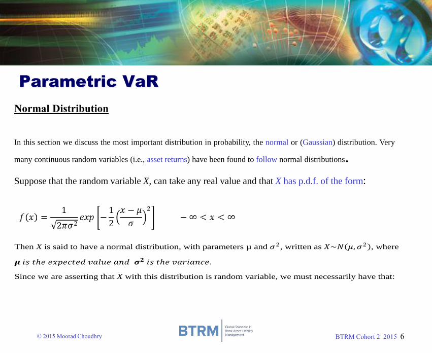
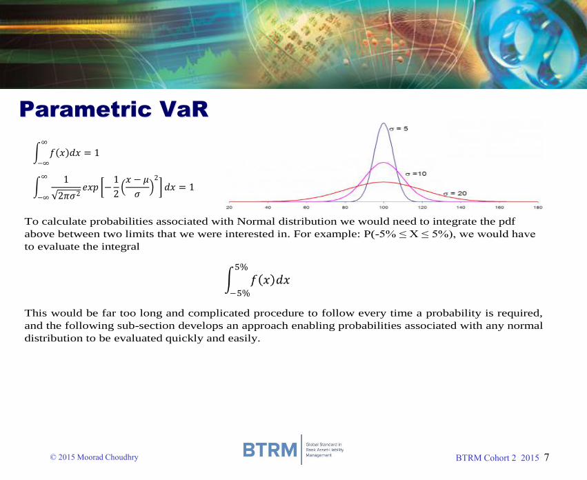
Suppose that the random variable X, can take any real value and that X has p.d.f. of the form:
In this section we discuss the most important distribution in probability, the normal or (Gaussian) distribution. Very
many continuous random variables (i.e., asset returns) have been found to follow normal distributions.
Then X is said to have a normal distribution, with parameters µ and 𝜎2, written as 𝑋~𝑁 𝜇,𝜎2 , where
𝝁 𝑖𝑠 𝑡ℎ𝑒 𝑒𝑥𝑝𝑒𝑐𝑡𝑒𝑑 𝑣𝑎𝑙𝑢𝑒 𝑎𝑛𝑑 𝝈𝟐 𝑖𝑠 𝑡ℎ𝑒 𝑣𝑎𝑟𝑖𝑎𝑛𝑐𝑒.
Since we are asserting that X with this distribution is random variable, we must necessarily have that:
Normal Distribution
BTRM Cohort 2 2015 7© 2015 Moorad Choudhry
Parametric VaR
𝑓 𝑥 𝑑𝑥 = 1∞
−∞
1
2𝜋𝜎2𝑒𝑥𝑝 −
1
2 𝑥 − 𝜇
𝜎
2
𝑑𝑥 = 1∞
−∞
To calculate probabilities associated with Normal distribution we would need to integrate the pdf
above between two limits that we were interested in. For example: P(-5% ≤ X ≤ 5%), we would have
to evaluate the integral
This would be far too long and complicated procedure to follow every time a probability is required,
and the following sub-section develops an approach enabling probabilities associated with any normal
distribution to be evaluated quickly and easily.

BTRM Cohort 2 2015 8© 2015 Moorad Choudhry
Parametric VaR
Standard Normal Distribution
We do the following transformation:
A normal distribution having = 0 and 2 = 1 is called standard normal distribution.
Therefore, if 𝑍~𝑁 0, 1 , then the distribution function of standard normal function is given by;
𝜑 𝑍 = 𝑃 𝑍 ≤ 𝑧 =1
2𝜋 𝑒𝑥𝑝 −
1
2 𝑥 2 𝑑𝑥
𝑧
−∞
)1,0(N
Suppose that Z has the standard Normal distribution, Z ~ )1,0(N . Then we will use Standard
cumulative distribution table to find probabilities:
BTRM Cohort 2 2015 9© 2015 Moorad Choudhry
Parametric VaR
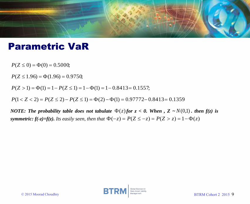
;5000.0)0()0( ZP
;9750.0)96.1()96.1( ZP
;1557.08413.01)1(1)1(1)1()1( ZPZP
1359.08413.097772.0)1()2()1()2()21( ZPZPZP
NOTE: The probability table does not tabulate )(z for z < 0. When , Z ~ )1,0(N . then f(z) is
symmetric: f(-z)=f(z). Its easily seen, then that )(1)()()( zzZPzZPz
BTRM Cohort 2 2015 10© 2015 Moorad Choudhry
Parametric VaR
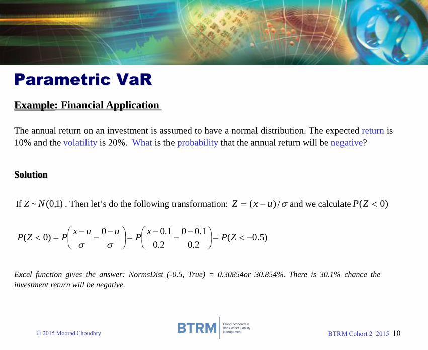
Example: Financial Application
The annual return on an investment is assumed to have a normal distribution. The expected return is
10% and the volatility is 20%. What is the probability that the annual return will be negative?
Solution
If Z ~ )1,0(N . Then let’s do the following transformation: /)( uxZ and we calculate )0( ZP
)5.0(2.0
1.00
2.0
1.00)0(
ZP
xP
uuxPZP
Excel function gives the answer: NormsDist (-0.5, True) = 0.30854or 30.854%. There is 30.1% chance the
investment return will be negative.
BTRM Cohort 2 2015 11© 2015 Moorad Choudhry
Parametric VaR
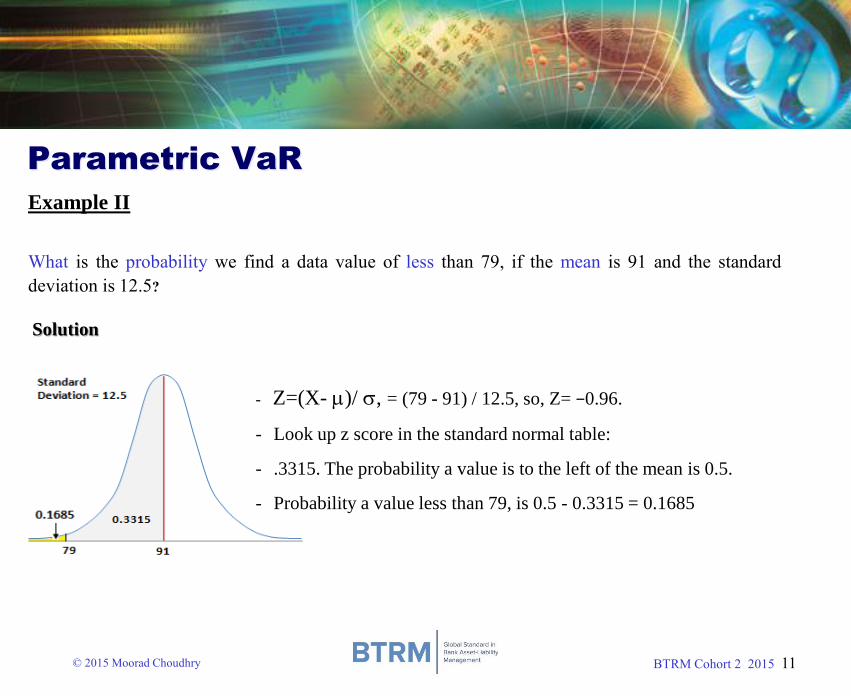
What is the probability we find a data value of less than 79, if the mean is 91 and the standard
deviation is 12.5?
Solution
- Z=(X- )/ , = (79 - 91) / 12.5, so, Z= −0.96.
- Look up z score in the standard normal table:
- .3315. The probability a value is to the left of the mean is 0.5.
- Probability a value less than 79, is 0.5 - 0.3315 = 0.1685
Example II
BTRM Cohort 2 2015 12© 2015 Moorad Choudhry
Parametric VaR
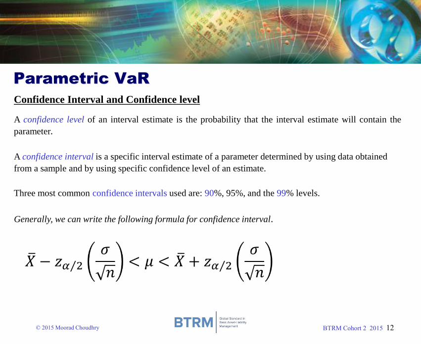
Confidence Interval and Confidence level
A confidence level of an interval estimate is the probability that the interval estimate will contain the
parameter.
A confidence interval is a specific interval estimate of a parameter determined by using data obtained
from a sample and by using specific confidence level of an estimate.
Three most common confidence intervals used are: 90%, 95%, and the 99% levels.
Generally, we can write the following formula for confidence interval.

BTRM Cohort 2 2015 13© 2015 Moorad Choudhry
Parametric VaR
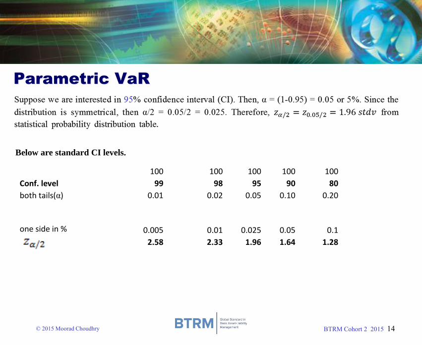
In general,
α = (1-CI). At 95% CI, then, α = (1-0.95) = 5% or 0.05. α/2 = 0.05/2 = 0.025. 𝑧0.05/2 = 1.96
α = (1-CI). At 99% CI, then, α = (1-0.99) = 0.1% or 0.01. α/2 = 0.01/2 = 0.005. 𝑧0.01/2 = 2.58
α = (1-CI). At 98% CI, then, α = (1-0.98) = 0.2% or 0.02. α/2 = 0.02/2 = 0.01. 𝑧0.02/2= 2.33
BTRM Cohort 2 2015 14© 2015 Moorad Choudhry
Parametric VaR
Below are standard CI levels.
100 100 100 100 100
Conf. level 99 98 95 90 80
both tails(α) 0.01 0.02 0.05 0.10 0.20
one side in %
0.005 0.01 0.025 0.05 0.1
2.58 2.33 1.96 1.64 1.28

BTRM Cohort 2 2015 15© 2015 Moorad Choudhry
Estimating Volatility
Volatility is a measure of capturing the variability of a given data set from its average (mean). It measures
the dispersion of the data around its mean.
Most common estimate of volatility is:
BTRM Cohort 2 2015 16© 2015 Moorad Choudhry
Compute VaR
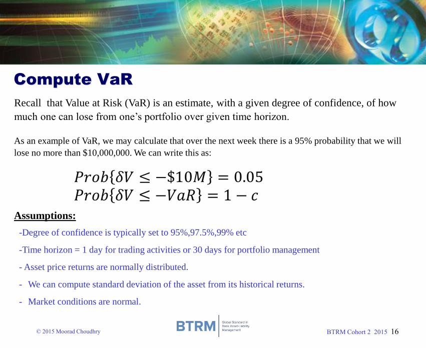
Recall that Value at Risk (VaR) is an estimate, with a given degree of confidence, of how
much one can lose from one’s portfolio over given time horizon.
As an example of VaR, we may calculate that over the next week there is a 95% probability that we will
lose no more than $10,000,000. We can write this as:
Assumptions:
-Degree of confidence is typically set to 95%,97.5%,99% etc
-Time horizon = 1 day for trading activities or 30 days for portfolio management
- Asset price returns are normally distributed.
- We can compute standard deviation of the asset from its historical returns.
- Market conditions are normal.
BTRM Cohort 2 2015 17© 2015 Moorad Choudhry
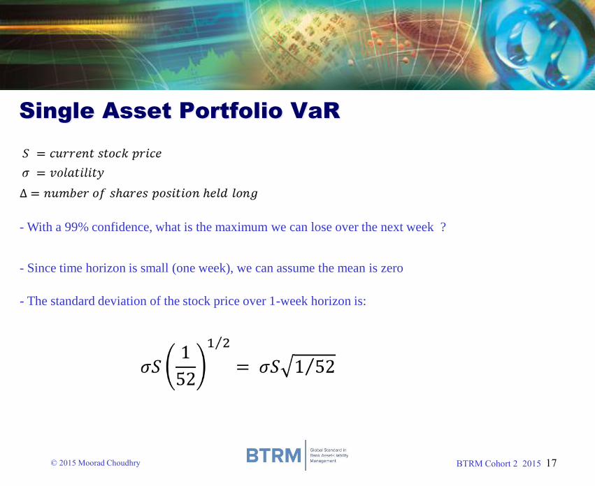
Single Asset Portfolio VaR
- With a 99% confidence, what is the maximum we can lose over the next week ?
- Since time horizon is small (one week), we can assume the mean is zero
- The standard deviation of the stock price over 1-week horizon is:
BTRM Cohort 2 2015 18© 2015 Moorad Choudhry
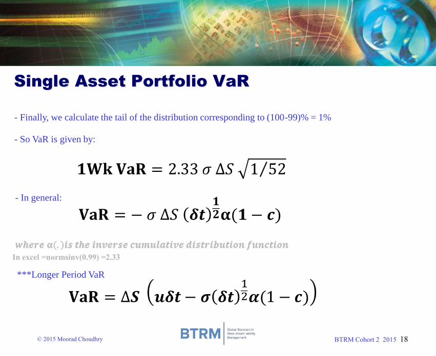
Single Asset Portfolio VaR
- Finally, we calculate the tail of the distribution corresponding to (100-99)% = 1%
- So VaR is given by:
In excel =normsinv(0.99) =2.33
- In general:
***Longer Period VaR

BTRM Cohort 2 2015 19© 2015 Moorad Choudhry
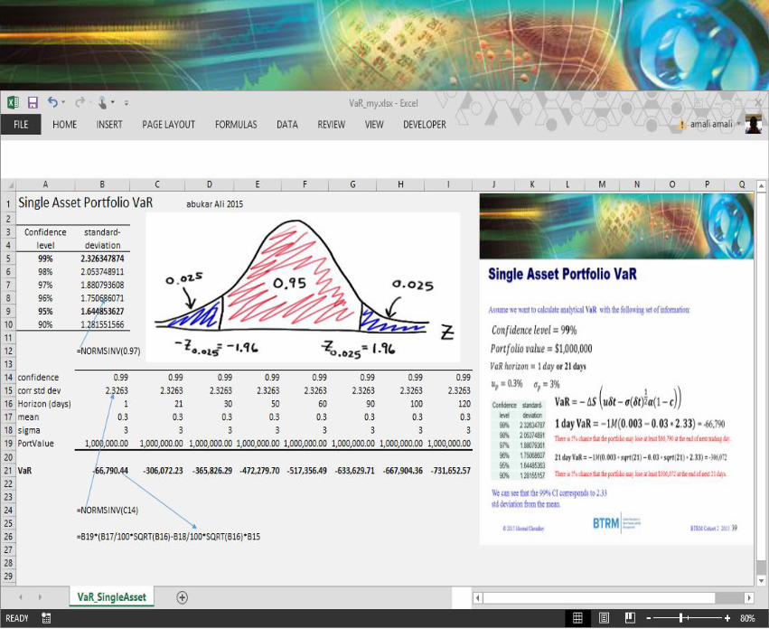
Single Asset Portfolio VaR
Assume we want to calculate analytical VaR with the following set of information:
Confidence standard-
level deviation
99% 2.32634787
98% 2.05374891
97% 1.88079361
96% 1.75068607
95% 1.64485363
90% 1.28155157
We can see that the 95% CI corresponds to1.64485
std deviation from the mean.
There is 5% chance that the portfolio may lose at least $46,435 at the end of next trading day.
There is 5% chance that the portfolio may lose at least $212,388 at the end of next 21 days.
BTRM Cohort 2 2015 20© 2015 Moorad Choudhry
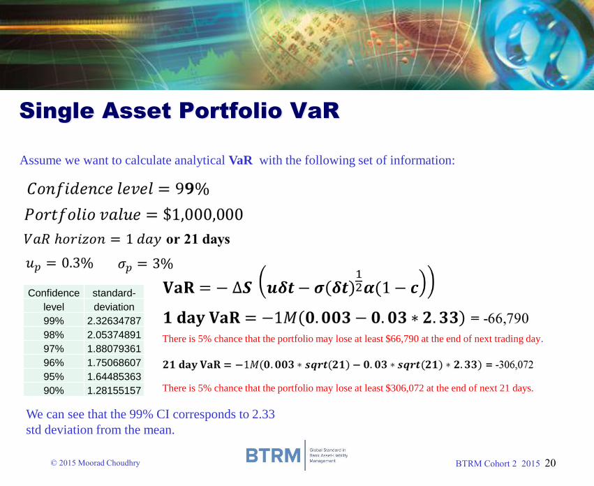
Single Asset Portfolio VaR
Assume we want to calculate analytical VaR with the following set of information:
Confidence standard-
level deviation
99% 2.32634787
98% 2.05374891
97% 1.88079361
96% 1.75068607
95% 1.64485363
90% 1.28155157
We can see that the 99% CI corresponds to 2.33
std deviation from the mean.
There is 5% chance that the portfolio may lose at least $66,790 at the end of next trading day.
There is 5% chance that the portfolio may lose at least $306,072 at the end of next 21 days.
BTRM Cohort 2 2015 21© 2015 Moorad Choudhry
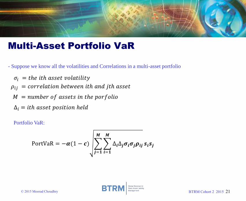
Multi-Asset Portfolio VaR
- Suppose we know all the volatilities and Correlations in a multi-asset portfolio
Portfolio VaR:
BTRM Cohort 2 2015 22© 2015 Moorad Choudhry
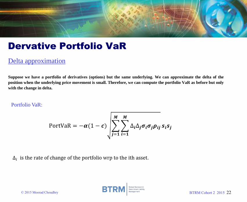
Dervative Portfolio VaR
Delta approximation
Portfolio VaR:
Suppose we have a portfolio of derivatives (options) but the same underlying. We can approximate the delta of the
position when the underlying price movement is small. Therefore, we can compute the portfolio VaR as before but only
with the change in delta.
BTRM Cohort 2 2015 23© 2015 Moorad Choudhry
Excel Calculations.
BTRM Cohort 2 2015 24© 2015 Moorad Choudhry
For discussion
What are the issues associated with understanding and “using” VaR in
the right way?
How did VaR as an estimation tool perform with respect to the 2008
crash and the JPMorgan “London Whale” episode?
BTRM Cohort 2 2015 25© 2015 Moorad Choudhry
References
John C Hull, “Options Futures and Other Derivatives”, 5th edition, 2003
Wilmott, P. “Paul Wilmott introduces quantitative finance.2001
Philipe Jorion, “Value at Risk”, 2nd edition, McGraw-Hill , 2001
Comments, any questions from this lecture or more information about full introduction to mathematical finance
lecture(s), please email me: [email protected]
BTRM Cohort 2 2015 26© 2015 Moorad Choudhry
DISCLAIMER
The material in this presentation is based on information that we consider reliable, but we do not
warrant that it is accurate or complete, and it should not be relied on as such. Opinions expressed
are current opinions only. We are not soliciting any action based upon this material. Neither the
author, his employers, any operating arm of his employers nor any affiliated body can be held liable
or responsible for any outcomes resulting from actions arising as a result of delivering this
presentation. This presentation does not constitute investment advice nor should it be considered
as such.
The views expressed in this presentation represent those of Abukar Ali in his individual private
capacity and should not be taken to be the views of any employer or any affiliated body, including
Abukar Ali as an employee of any institution or affiliated body. Either he or his employers may or
may not hold, or have recently held, a position in any security identified in this document.
This presentation is © [Abukar Ali] 2015. No part of this presentation may be copied,
reproduced, distributed or stored in any form including electronically without express written
permission in advance from the author.