variational electrodynamics of atoms jayme de luca · variational electrodynamics as an extension...

Progress In Electromagnetics Research B, Vol. 53, 147–186, 2013

VARIATIONAL ELECTRODYNAMICS OF ATOMS

Jayme De Luca *

Departamento de Fısica, Universidade Federal de Sao Carlos, RodoviaWashington Luis, km 235, Caixa Postal 676, Sao Carlos, SaoPaulo 13565-905, Brazil

Abstract—We generalize Wheeler-Feynman electrodynamics witha variational problem for trajectories that are required to mergecontinuously into given past and future boundary segments. Weprove that the boundary-value problem is well posed for twoclasses of boundary data. The well-posed solution in generalhas velocity discontinuities, henceforth a broken extremum. Alongregular segments, broken extrema satisfy the Euler-Lagrange neutraldifferential delay equations with state-dependent deviating arguments.At points where velocities are discontinuous, broken extrema satisfythe Weierstrass-Erdmann conditions that energies and momenta arecontinuous. Electromagnetic fields of the finite trajectory segments arederived quantities that can be extended to a bounded region B of space-time. Extrema with a finite number N of velocity discontinuities haveextended fields defined in B with the possible exception of N sphericalsurfaces, and satisfy the integral laws of classical electrodynamicsfor most surfaces and curves inside B. As an application, we studythe hydrogenoid atomic model with mass ratio varying by threeorders of magnitude to include hydrogen, muonium and positronium.For each model we construct globally bounded trajectories withvanishing far-fields using periodic perturbations of circular orbits. Ourmodel uses solutions of the neutral differential delay equations alongregular segments and a variational approximation for the head-oncollisional segments. Each hydrogenoid model predicts a discrete setof finitely measured neighbourhoods of periodic orbits with vanishingfar-fields right at the correct atomic magnitude and in quantitativeand qualitative agreement with experiment and quantum mechanics.The spacings between consecutive discrete angular momenta agree withPlanck’s constant within thirty-percent, while orbital frequencies agreewith a corresponding spectroscopic line within a few percent.

Received 12 May 2013, Accepted 6 July 2013, Scheduled 18 July 2013* Corresponding author: Jayme De Luca ([email protected]).

148 De Luca

1. INTRODUCTION

We generalize Wheeler-Feynman electrodynamics [1, 2] with avariational principle whose extrema are required to satisfy a boundary-value problem [3, 4]. As in all variational problems, there is noguarantee that smooth classical solutions exist. In fact, here weprove that one should expect piecewise smooth extrema. For genericboundary data, solutions are continuous trajectories with velocitydiscontinuity points, henceforth corner points [5].

Piecewise smooth extrema satisfy the Wheeler-Feynman neutraldifferential delay equations with state-dependent deviating argumentsalong smooth segments [3, 4]. At corner points piecewise smoothextrema satisfy the Weierstrass-Erdmann conditions that partialenergies and momenta are continuous [5].

For two special classes of boundary data we prove that thevariational principle is well-posed, i.e., there exists a unique solutiondepending continuously on the boundary data. The piecewise smoothsolutions define generalized electromagnetic fields inside a boundedregion B of space-time by extension. We show that the extendedfields satisfy the integral laws of classical electrodynamics inside B,i.e., Gauss’s surface integral law for the electric field, Gauss’s surfaceintegral law for the magnetic field, Ampere’s law and Faraday’sinduction law in integral form [6].

Wheeler and Feynman derived neutral differential delay equationsof motion (NDDE) for point charges [1, 2]. Neutral differentialdelay equations are functional differential equations whose qualitativebehaviour has just begun to be understood [7–9]. In qualitativeagreement with the existence of broken extrema, solutions of NDDEmust be defined piecewise [4]. The continuation of solutions oftenleaves a set of points where trajectories are not differentiable [8]. Inthe numerical analysis literature, a velocity discontinuity point is calleda breaking point [8], while in variational calculus (and here) the namecorner point is used [5].

Surprisingly, atomic models become sensible in variationalelectrodynamics. More specifically, our generalized electrodynamicsallows globally bounded two-body orbits with vanishing far-fields, thusintroducing bounded motions along which an atom is isolated fromdisturbing/being disturbed by other atoms. The essential ingredientis precisely corner points. It is proved in [4] that globally boundedtwo-body orbits with vanishing far-fields must have corner points. Weattempt to validate our theory by exploring the hydrogenoid atomicmodel with mass-ratio varying by three orders of magnitude to includethe hydrogen, muonium and positronium atoms.

Progress In Electromagnetics Research B, Vol. 53, 2013 149

We construct periodic orbits having regular segments wherethe neutral differential delay equations and deviating arguments arelinearized, while on the (thin) boundary-layer segments a variationalapproximation is used.

In the three cases of hydrogen, muonium and positronium,a discrete set of finitely measured neighbourhoods of orbits withvanishing far-fields have frequencies in agreement with QuantumMechanics (QM), within a few percent. The qualitative agreementswith QM are (i) the angular momenta of the unperturbed circularorbits are approximately integer multiples of a basic angularmomentum agreeing with Planck’s constant within thirty percent;(ii) the emitted frequency is the difference of two eigenvalues of asuitable linear problem; and (iii) the Weierstrass-Erdmann conditionsinvolve the continuity of momenta and energies, which are the relevantquantities of QM.

This paper is divided as follows. In Section 2, we introducethe boundary-value problem, the variational structure, and theWeierstrass-Erdmann conditions. In Section 3, we prove that theboundary-value problem is well-posed. In Section 4, we explainvariational electrodynamics as an extension of Wheeler-Feynmanelectrodynamics by discussing the conditions for the validity ofthe integral laws, which are the experimental basis of classicalelectrodynamics. Section 4 also discusses invariant manifolds anda generalized absorber condition. In Section 5, we introduce thecircular orbits and magnitudes in the limit of small delay angles. InSection 6, we linearize the Wheeler-Feynman NDDE about circularorbits and explain the infinite number of linearly unstable transversalmodes. Section 7 discusses the boundary-layer theory and applicationof the Weierstrass-Erdmann conditions. In Section 8, we validate ourtheory by comparing the predictions of the hydrogenoid model withthe experimental magnitudes of hydrogen, muonium and positronium.Last, in Section 9, we put the discussions and conclusion.

2. BOUNDARY-VALUE PROBLEM

We henceforth use a unit system where the speed of light is c ≡ 1 andthe electronic charge and electronic mass are respectively e1 ≡ −1 andm1 ≡ 1. The protonic charge and protonic mass in our unit systemturn out to be respectively e2 = 1 and m2 = 1836.1526.

A seemingly essential ingredient for a viable physical (andmathematical) theory is the minimization of a suitably definedfunctional, henceforth a variational principle. A useful paradigm isthe principle of least action of classical mechanics specialized to the

150 De Luca

Kepler two-body problem [10]. Hamilton’s principle states that theaction functional assumes an extremum on the classical two-body orbitof a finite time-interval, when considered in the class of C2 smoothtrajectories sharing the same endpoints.

The principle of least action [10] defines a two-point boundaryproblem for the ordinary differential equations (ODE) of classicalmechanics [11, 12], often called a shooting problem to distinguishfrom the initial value problem [11, 12]. Motivated by Wheeler-Feynman electrodynamics, Ref. [3] constructed a Poincare-invariantaction principle at the expense of introducing the unusual boundaryconditions explained below.

Physical trajectories should have a velocity lesser than the speed oflight, henceforth sub-luminal trajectories. We describe our relativistictrajectories in the usual Minkowski space, where every point P ≡ (t,x)has a time and a Cartesian coordinate [3, 13]. A point P+ ≡ (tj+,xj+)belongs to the future of P when tj+ > t+‖xj+−x‖, while a point P− ≡(tj−,xj−) belongs to the past of P when tj− < t−‖xj−−x‖ [13]. Theset of points neither in the future of P nor in the past of P is definedas the elsewhere of P [13]. A point P± along trajectory xj ≡ xj(tj) isin the light-cone relation with another point P if

tj± = t± ‖xj±(tj±)− x‖. (1)Equation (1) is an implicit state-dependency on xj(tj±), henceforththe light-cone condition or the Einstein locality condition. In Eq. (1),the plus sign defines the future light-cone of P and the minus signdefines the past light-cone of P .

To continue trajectory 1 from an initial point O1 ≡ (tO1 ,x1(tO1)),a relativistic variational principle needs the whole intersection oftrajectory 2 with the elsewhere of O1, which is a finite segment oftrajectory 2. For the classical principle of least action, the elsewhereof O1 degenerates into the initial point of trajectory 2. Last, at theend-point L2 of trajectory 2, the relativistic least-action principle needsthe intersection of trajectory 1 with the elsewhere of L2, again a finitesegment of trajectory 1 rather than a simple endpoint.

The unusual boundary conditions for a relativistic variationalprinciple are illustrated in Fig. 1, i.e., (a) the initial point O1 oftrajectory 1 and the respective boundary-segment of trajectory 2 insidethe light-cone of O1 (red triangle of Fig. 1), and (b) the final point L2 oftrajectory 2 and the corresponding boundary-segment of trajectory 1inside the light-cone of L2 (upside down red triangle of Fig. 1).

Along continuous and piecewise C1 sub-luminal trajectoriessatisfying the boundaries of Fig. 1, the past and future light-coneconditions (1) have unique solutions tj±(t,x) [14]. Illustrated in Fig. 1are also the forward light-cone rays starting from O+

1 and moving


O1

O+

1O

+

1L

2

L2

+L

2

+

b3

1

b2

f3

f2a

+

2

a+

1

f1

a11

a21

a12

a22

Figure 1. Schematic illustration of the boundaries in R4, i.e.,(a) initial point O1 ≡ (tO1 ,x1(tO1)) of trajectory 1 and the respectiveelsewhere boundary segment of x2(t2) for t2 ∈ [tO−1 , tO+

1] (solid red

line); (b) endpoint L2 ≡ (tL2 ,x2(tL2)) of trajectory 2 and the respectiveelsewhere boundary segment of x1(t1) for t1 ∈ [tL−2 , tL+

2] (solid red

line). Trajectories x1(t1) for t1 ∈ [tO1 , tL−2] (solid blue line) and x2(t2)

for t2 ∈ [tO+1, tL2 ] (solid green line) are determined by the extremum

condition. The principal sewing chains are also illustrated; i.e., theforward sewing chain of O+

1 , (O+1 , f1, f2, f3), (broken golden line)

and the backwards sewing chain of L−2 , (L−2 , b1, b2, b3) (broken darkline). Sewing chain (a−2 , a11, a21, a12, a22, a

+1 ) has two points on each

trajectory (solid violet line). Violet arrows are directions of integrationto be explained below. Arbitrary units.

with the future light-cone condition (1) to f1, f2 and f3, and thebackwards light-cone rays starting from L−2 and moving with the pastlight-cone condition (1) to b1, b2 and b3, henceforth called the forwardand backward principal sewing chains, respectively.

The action functional is a sum of four integrals: two localintegrals each involving one trajectory,

∫Ti(xi, xi)dti; and two

interaction integrals depending on both positions and velocities, whereone position/velocity is evaluated at a deviating time argument,∫

V ±ij (xi, xi,xj±, xj±)dti. The action functional can be expressed in

152 De Luca

two equivalent forms, i.e.,

S ≡∫ tL2

tO+

1

T2dt2 +∫ t

L−2

tO1

T1dt1 +∫ t

L+2

tO1

V −12dt1

︸︷︷︸+

∫ tL−2

tO1

V +12dt1

︸︷︷︸, (2)

‖ ‖

=∫ t

L−2

tO1

T1dt1 +∫ tL2

tO+

1

T2dt2 +

︷︸︸︷∫ tL2

tO−1

V +21dt2 +

︷︸︸︷∫ tL2

tO+

1

V −21dt2, (3)

where vertical braces under each interaction integral indicateequivalence by a change of the integration variable. The Jacobian foreach change of variable from ti to tj±(ti) is equal to the derivative ofthe delayed time tj±(ti,xj(ti)) evaluated along the orbit, as obtainedtaking a derivative of the implicit condition (1) with x ≡ xi(ti),

dtj±dti

=(1± nj± · vi)

(1± nj± · vj±), (4)

and explained in Refs. [3, 14]. One can thus express the interactionterms by either integrals over t1 (Eq. (2)) or by integrals over t2(Eq. (3)). In principle, an arbitrary variational structure couldbe defined using generic V ′s on line (2), which would in turndetermine the V ′s on line (3) by changing variables with (4) or theequivalent Jacobian if the constraints were other than the light-coneconditions (1).

Here we consider only the variational structure defined byconstraints (1) and functionals (2) and (3) with

Ti ≡ mi

(1−

√1− v2

i

), (5)

V ±ij (xi, xi,xj±, xj±) ≡ − eiej(1− vi · vj±)

2rj±(1± nj± · vj±), (6)

where j ≡ 3 − i and i = 1, 2; henceforth variational electrodynamics.For the hydrogenoid problem we henceforth replace eiej ≡ −1 andcarry an arbitrary protonic mass, for which case V ±

12 ≥ 0 and V ±21 ≥ 0,

thus defining a semi-bounded action functional (2) (S ≥ 0).The variational problem is to find the trajectory segments

(O1, L−2 ) (blue) and (O+

1 , L2) (green) between the endpoints of Fig. 1.For the linear variation, trajectory 2 is to be kept fixed whiletrajectory 1 is varied, and line (2) with the first term kept constantdefines partial Lagrangian 1. Vice-versa, trajectory 1 is to be keptfixed while trajectory 2 is varied, and line (3) with the first term frozendefines partial Lagrangian 2.


Next we discuss acceptable trajectories for the variationalproblem. The classical calculus of variations requires at least aneighbourhood in a normed space of piecewise-smooth continuoustrajectories [5]. Specific difficulties are (i) along acceptable trajectoriessatisfying the boundaries of Fig. 1, functionals (2) and (3) requireexistence of unique advanced/retarded arguments t2±(t1), ∀ t1 ∈[tO1 , tL+

2] and t1±(t2), ∀ t2 ∈ [tO−1 , tL2 ]; and (ii) functional-analytic

results require a whole domain in which functionals (2) and (3) arewell defined, e.g., a normed linear space.

To satisfy (i) a neighbourhood of C1 smooth sub-luminaltrajectories suffices, as guaranteed by Lemma 1 of Ref. [14]. Weremark that Lemma 1 of [14] can be extended to continuous trajectoriesthat are sub-luminal almost everywhere, a measure-theoretic extensionnot pursued here. As regards (ii) we notice that the integrands offunctionals (2) and (3) include denominators that should be non-zerooutside sets of zero measure, as discussed in Ref. [15] for the Keplerproblem.

To study critical points using the modern topological theo-rems [16, 17] would require a reflexive space (Banach or Hilbert),where (2) and (3) are finitely integrable [15] and Frechet differen-tiable [17]. Such ambitious goal is beyond the present work. Hence-forth we study functional minimization restricted to neighbourhoodsof non-collisional sub-luminal trajectories, along which the denomina-tors of (2) and (3) are everywhere finite. The topology used is that ofthe normed space of continuous and piecewise C2 functions, henceforthC2.

For C2 smooth extrema, the critical point conditions are theEuler-Lagrange equations of the integrands of Eqs. (2) and (3) withthe respective first term dropped, henceforth the partial Lagrangiansdefined by

Li ≡ Ti − vi ·Aj + Uj , (7)

where

Aj ≡ vj−2rj−(1− nj− · vj−)

+vj+

2rj+(1 + nj+ · vj+),

Uj ≡ 12rj−(1− nj− · vj−)

+1

2rj+(1 + nj+ · vj+),

for j ≡ 3 − i and i = 1, 2. In Eq. (7), Aj is the vector potential ofparticle j.

The Euler-Lagrange equation of the above defined Li yields the

154 De Luca

Lorentz-force law (the equation of motion of Wheeler and Feynman)

mid

dt

vi√

1− v2i

= ei(Ej(t,xi) + vi ×Bj(t,xi)), (8)

for i = 1, 2 [1, 2]. In Eq. (8), the Lienard-Wiechert fields of the othercharge (j ≡ 3− i) are

Ej(t,x) ≡ 12(Ej+ + Ej−), (9)

Bj(t,x) ≡ 12(Bj+ + Bj−), (10)

with

Ej±(t,x) ≡ ej

uj±

γ2j±r2

j±+

nj± × (uj± × aj±)rj±

, (11)

uj±(t,x) ≡ (nj± ± vj±)(1± nj± · vj±)3

, (12)

Bj±(t,x) ≡ ∓nj± ×Ej±, (13)

where γj± ≡ (1 − v2j±)−1/2, and vj± ≡ dxj/dt|t=tj± and aj± ≡

d2xj/dt2|t=tj± are the velocity and acceleration of charge j evaluated atthe advanced/retarded times tj± defined by Eq. (1). Last, in Eq. (11)the distance in light-cone is a scalar function of (t,x) defined by

rj± ≡ ‖x− xj(tj±)‖, (14)

and

nj± ≡ (x− xj(tj±))/rj±, (15)

is a unit vector from position xj(tj±) to point x [1, 2, 6]. Eq. (8) isa neutral differential delay equation (NDDE) with state-dependentdeviating arguments [1, 2, 4].

In the following we study the wider class of piecewise smoothcontinuous extrema having a finite number of corner points, henceforthbroken extrema [5]. Piecewise smooth extrema have the followingnice properties: (i) inside intervals where trajectory and deviatingarguments are C2 smooth, broken extrema satisfy the Euler-LagrangeEq. (8); and (ii) at corner points extremal trajectories satisfy theWeierstrass-Erdmann conditions explained below [5].


The first Weierstrass-Erdmann condition [5] is the continuity ofthe momentum of partial Lagrangian i (as defined by Eq. (7)), i.e.,

∂Li

∂vi=

mivi√1− v2

i

− vj−2rj−(1− nj− · vj−)

− vj+

2rj+(1 + nj+ · vj+), (16)

=mivi√1− v2

i

−Aj . (17)

Notice that Eq. (16) includes the past/future velocities of chargej ≡ 3− i. Should the extremal trajectory of particle i have a velocitydiscontinuity at time ti, the trajectory of particle j must compensatewith a corner point in light-cone at either tj− or tj+, in order to makethe right-hand-side of (16) continuous.

Here we use the name partial energy to distinguish from theconstant value of the Hamiltonian along a Hamiltonian dynamics.After the no-interaction theorem [18, 19] we know that a finite-dimensional Hamiltonian does not exist for the electromagnetic two-body problem, even though partial energies are introduced below byan energy-looking formula.

The partial energy of partial Lagrangian (7) is defined by

Ei ≡ vi · ∂Li

∂vi−Li =

mi√1− v2

i

− Uj . (18)

The second Weierstrass-Erdmann condition [5] is that the partialenergy (18) is continuous across each corner point. In Eq. (18) indexj is defined by the usual j ≡ 3 − i, e.g., for i = 2 we have j = 1. Westress that the Ei in Eq. (18) are not constants of the motion. Thepartial energy is a property of each particular corner (perhaps differentfor different corners). Each Ei is conserved only across a particularcorner in the sense of having the same value to the left and to the rightof that corner.

To express the vanishing of the momentum jump (17) across acorner point we introduce an upper index l or r to indicate respectivelyleft-velocity or right-velocity at the breaking point. Using Eq. (18) toeliminate the mechanical momentum from Eq. (16), we obtain the

156 De Luca

combined necessary condition for a corner point,

∆(

∂Li

∂vi

)= Ei∆vi +

∆vi −

(nj− · vl

j−)vr

i +(nj− · vr

j−)vl

i

2rj−(1− nj− · vl

j−)(

1− nj− · vrj−

)

+

∆vi +

(nj+ · vl

j+

)vr

i −(nj+ · vr

j+

)vl

i

2rj+

(1 + nj+ · vl

j+

)(1 + nj+ · vr

j+

)

− ∆vj− − nj− ×

(vr

j− × vlj−

)

2rj−(1− nj− · vl

j−)(

1− nj− · vrj−

)

− ∆vj+ + nj+ ×

(vr

j+ × vlj+

)

2rj+

(1 + nj+ · vl

j+

)(1 + nj+ · vr

j+

) ≡ 0, (19)

where ∆vi ≡ vri − vl

i, ∆vj± ≡ vrj± − vl

j± and j ≡ 3 − i. Eq. (19) isa nonlinear condition for the jumping velocities, a necessary conditioninvolving the Ei to be adjusted such that (18) is continuous at thatcorner. In Section 3, Eq. (19) is linearized for small jumps by replacingvr

i → vli+∆vi and vr

j± → vlj±+∆vj± and expanding up to linear order

on the ∆vi , in which case the partial energies appear as eigenvaluesof the linearized problem (19). In Section 7, the fully nonlinearcondition (19) is used.

3. WELL-POSEDNESS

As mentioned in [3, 14] and illustrated in Fig. 2, the shortest-lengthboundary-value problem is when L−2 is in the forward light-cone ofO+

1 . Otherwise, the supposedly independent past and future historiesinteract in light-cone, an absurdity.

In the following we give a pedestrian existence proof that theboundary-value problem is well-posed for C2 boundary segments ofthe above defined shortest length. We further assume boundarysegments sufficiently close to segments of circular orbits of small-delay-angles [20], and define continuity with the C2 topology of continuousand piecewise C2 functions.

It is instructive to translate the schematics of Fig. 1 and Fig. 2 interms of the magnitudes of circular orbits with small delay angles,whose light-cone-distance is rb ≡ 1/µθ2, (Eq. (33)), and velocity|v| ' θ ¿ 1, (Eq. (35)). The time span of each circular trajectory


O1

O+

1O

1 L2

L2L

2

+

a1

a+

1

a2

a2

_

_ _

Figure 2. Schematic illustration of the point-plus-elsewhere-boundary-segments in R4 for the boundary value problem of shortestlength, i.e., (a) initial point O1 ≡ (tO1 ,x1(tO1)) of trajectory 1 andthe respective elsewhere boundary segment of x2(t2) for t2 ∈ [tO−1 , tO+

1]

(solid red line); and (b) endpoint L2 ≡ (tL2 ,x2(tL2)) of trajectory 2 andthe respective elsewhere boundary segment x1(t1) for t1 ∈ [tL−2 , tL+

2]

(solid red line). Trajectories x1(t1) for t1 ∈ [tO1 , tL−2] (solid blue line)

and x2(t2) for t2 ∈ [tO+1, tL2 ] (solid green line) are determined by the

extremum condition. Sewing chain (a−2 , a1, a2, a+1 ) from a1 along

trajectory 1 and moves (forward and backwards) until the boundarysegments (solid violet line).

of Fig. 2 is ∆tj ≡ tL−2− tO1 = tO+

1− tL2 = 2rb, for j = 1, 2 (blue

and green segments). The shortest time of flight is two light-conedistances rb, and for small θ these are almost straight-line constant-velocity trajectories (Fig. 4 with small θ).

The two-point-boundary-value problem with ∆tj = 2rb is relatedto the initial value problem by a linear one-to-one map, i.e., x(∆t) =x(0) +

∫ ∆t0 v(t′)dt ' x(0) + 2rbv(0) [12]. Below we are dealing with

small perturbations of the former map, in which case the implicitfunction theorem allows one to control the end-point by adjusting theinitial velocity.

Theorem I: (i) For C2 boundaries of shortest-length (Fig. 2),the unique solution depends continuously on boundary data thatare sufficiently close to segments of a small-delay-angle circular orbit(again, continuity in the C2 topology). (ii) Generically, the velocities

158 De Luca

are discontinuous at O+1 and L−2 .

Proof : (i) As illustrated in Fig. 2, for the shortest-length case thepast light-cone of a1 falls on the past history segment, i.e., point a−2of Fig. 2. Likewise, the future light-cone of a2 is on the future historysegment (illustrated by a+

1 in Fig. 2). Next we write the equations foraccelerations a1 and a2, which interact in light-cone. The equations ofmotion (38) can be written as

m1a1√1− v2

1

= Aa2 + F−2 (x1,x2+,v1,v2+), (20)

m2a2√1− v2

2+

= Ba1 + F+1 (x2+,x1v2+,v1), (21)

where we have singled out the linear dependence on the other particle’srunning acceleration across the light-cone. In Eq. (20), vector F−2depends continuously on the past-history segment’s position, velocityand acceleration. Analogously, in Eq. (21), F+

1 depends continuouslyon the future history segment’s position, velocity and acceleration(again, continuity with the C2 topology).

Eliminating a2 from the right-hand-side of Eq. (20) with Eq. (21),and eliminating a1 from the right-hand-side of Eq. (21) with Eq. (20),yields (

m1I3 − 1m2AB

)a1 = F1 (x1,x2+,v1,v2+) , (22)

(m2I3 − 1

m1BA

)a2 = F2(x1,x2+,v1,v2+), (23)

where A ≡√

1− v21A, B ≡

√1− v2

2+B, and I3 is the 3 × 3 identitymatrix.

In Eqs. (22) and (23), vectors F1 and F2 depend continuously onboth history segments positions, velocities and accelerations. Nearsmall-delay-angle circular orbits the separation in light-cone r12 ≡|x1 − x2+| ' rb is large and A and B are O( 1

r12), such that for

r212 À 1

m1m2the matrices on the left-hand-sides of (22) and (23) are

non-singular quasi-diagonal matrices that can be inverted, yielding aLipshitz-continuous non-autonomous ODE for the accelerations.

The dominant linear dependence on accelerations is obtained fromthe far-field component of (11) in the approximation of Eq. (41), whichyields A = B = (1/r12)Q with Q an O(1) symmetric 3 × 3 matrixdepending only on the normal along the light-cone.

Last, points x2+ and x1 should evolve in the light-cone condition,and given that a2 ≡ dv2+/dt2+ and a1 ≡ dv1/dt1, a further


transformation using dt2+/dt1 as given by (4) is necessary to makeboth evolution parameters of (22) and (23) equal (a near-identitytransformation). Eqs. (22) and (23) must then be used with a two-point boundary problem by choosing initial velocities such that orbitsstarting from O1 and O+

1 hit L−2 and L2.(ii) The two-point boundary problem uses up all the adjustable

initial-positions and initial-velocities for ODE (22) and (23), and thereis no freedom left to adjust that the end velocities are continuouswith history velocities at O+

1 and L−2 . The case of perfectlycircular segments is exceptional due to the existence of the circularsolutions [20]. From circular boundary data, the above integrationsimply continues the C∞ circular solution. Otherwise, from genericnear-circular boundary data, the integration defines a near-circularorbit with velocity discontinuities at O+

1 and L−2 .As a bonus, the above construction shows that solutions with

discontinuous velocities are expected. For purely C2 segments thereare no Weierstrass-Erdmann conditions for shortest-length boundaries.Still for the shortest-length case, the above result can be generalizedfor boundary segments that are continuous and piecewise C2. Forthose, the ODE integration has to be stopped at every breaking pointto satisfy the Weierstrass-Erdmann conditions (19) that can be writtenas

m1∆v1√1− v2

1

=G1∆v2+

r12(1− (n · v2+)2)+ U2−∆v2−, (24)

m2∆v2+√1− v2

2+

=G2∆v1

r12(1− (n · v1)2)+ U1+∆v1+, (25)

as obtained substituting vrj± = vl

j±+∆vj± into Eq. (19). In Eqs. (24)and (25), G1 and G2 are O(1) 3 × 3 matrices and we have explicitlyintroduced the extra factors in the denominators, which should benear-one for low-velocity orbits. Still in Eqs. (24) and (25), matricesU2− and U1+ are bounded and depend continuously on the boundarysegments positions, velocities and accelerations. Eqs. (24) and (25)can be solved for the velocity discontinuities along the unknown orbitalsegments, ∆v1 and ∆v2+, yielding

(m1m2I3 − λG1G2)∆v1 = K11∆v2− + K12∆v1+, (26)

(m1m2I3 − λG2G1)∆v2+ = K21∆v2− + K22∆v1+, (27)

with

λ ≡√

1− v21

√1− v2

2+

r212 (1− (n · v1)2) (1− (n · v2+)2)

. (28)

160 De Luca

Theorem II: For continuous and piecewise C2 boundarysegments of shortest type, having a finite number of velocitydiscontinuities and sufficiently close to circular segments of λ ¿ m1m2

(λ defined in Eq. (28)), the boundary value problem is well-posed inthe C2 topology.

Proof: Every time the ODE integration of Theorem I is haltedbecause of a velocity discontinuity in a history segment, the ∆v1+ and∆v2− on the right-hand-side of Eqs. (26) and (27) are small becauseboundary segments are sufficiently close to circular segments. Giventhat λ ¿ m1m2, the matrices on the left-hand-sides of Eqs. (26)and (27) can be inverted, yielding small values for ∆v1 and ∆v2+.Eventually, the two-point-boundary-value problem yields an orbit stillclose to the circular segment.

The above constructed continuous trajectories have as many veloc-ity discontinuities as the combined past/future history segments have.Theorem II generalizes to boundary segments near constant-velocity-straight-line-segments at large separations and small velocities. Forboth circular and straight-line boundary segments, matrices Kij on theright-hand-side of Eqs. (26) and (27) fall as 1/r12 (not indicated), suchthat universal perturbations of distant charges decay with distance, asmentioned at the end of Section 4.

Notice that the quantity λ defined in Eq. (28) appeared earlier inEq. (67) of Section 7 in a completely different limit. For the periodicorbit of Section 7, the matrices on the left-hand-side of Eqs. (26)and (27) would be near-singular because the stepping-stone conditionis λ ≈ m1m2, but then the velocity jumps on the right-hand-sidesof (26) and (27) are not arbitrary because in Section 7 we are dealingwith a periodic orbit.

The problem of boundary segments with longer time-spansrequires inversion of larger matrices. Figure 1 illustrates a longerboundary-value problem (∆tj ' 3rb). Notice in Fig. 1 that sewingchains starting from points either on segment (O1,b2) or on segment(f1,L−2 ) have two vertices along trajectory 1, while sewing chainsstarting from points on the central segment (b2, f1) have just onevertex along trajectory 1. The situation of trajectory 2 is analogous.The Wheeler-Feynman advance/delay equations for accelerationsa11,a12,a21,a22 illustrated in Fig. 1, are obtained analogously to the


case of Theorem I, yielding

m1I3 0 Garb

00 m1I3 Gb

rb

GcrbGa

rb

Gbrb

m2I3 00 Gc

rb0 m2I3

a11

a12

a21

a22

= F(t1,X,V, boundary segments), (29)where X and V indicate positions and velocities of the four runningvertices of the sewing chain illustrated by solid violet lines in Fig. 1.

Theorem III: For near-circular C2 boundary segments with2rb < ∆tj < 4rb, the unique solution depends continuously onthe boundary data (with the C2 topology) and has two velocitydiscontinuities inside each trajectory of the solution segment, points(b1, f2) (green) and (b2, f1) (blue) of Fig. 1.

Proof: In Eq. (29), Ga,Gb and Gc are O(1) symmetric 3 × 3matrices, just like in Theorem I. Explained as an initial-value problemillustrated by violet arrows in Fig. 1, after the non-singular near-diagonal 12 × 12 symmetric matrix on the left-hand-side of Eq. (29)is inverted (for small λ), integration of ODE (29) should start fromx11(0) = xO1 , x21(0) = xO+

1, x12(0) = xf1 , x22(0) = xf2 .

The initial near-circular velocities and the initial positions (f1, f2)are not known unless for circular boundary segments. Otherwise, fornear-circular segments these must be chosen such that at the end-point(x12,x22) = (L−2 ,L2) and the running light-cone-ray (x11,x21) is ray(b2,b1) of the backwards sewing chain of L−2 .

The remaining central segments (b1, f2) (green) and (b2, f1) (blue)of Fig. 1 are done in the manner of Theorem I, generating velocitydiscontinuities at f1, f2, b1 and b2, which must satisfy Weierstrass-Erdmann conditions, one over each orbital corner of each principalsewing chain. Counting the end-point velocity discontinuities at O+

1

and L−2 , the generic case has six velocity discontinuities even for C2

boundaries.The above theorems suggest that the variational problem makes

sense at least in the neighbourhood of circular orbits [20]. Noticethat Eq. (29) is a non-autonomous ODE because the advanced andretarded arguments depend explicitly on the running time t1 via thelight-cone condition (1). The well-posedness of the general boundary-value problem is an open problem.

Last, the former theorems predicted a critical distance r212 ' 1

m1m2

below which the matrices can no longer be inverted and the equations

162 De Luca

of motion are differential-algebraic [12]. It is interesting to notice thatthe critical magnitude is of the order of the nuclear magnitude.

4. GENERALIZED WHEELER-FEYNMANELECTRODYNAMICS

Notice that Aj is defined by Eq. (17) only on points of the finitesegment of trajectory i illustrated in Fig. 1. To extend Aj to a fieldAj(t,x) we need tj− < t < tj+ for some tj− and tj+ belonging tothe finite segment of trajectory j illustrated in Fig. 1. For example,for j = 2 the light-cone distances defined by Eq. (14) evaluate tor2−(t,x) = t − t2− and r2+(t,x) = t2+ − t, which implies thatr2− + r2+ = t2+ − t2− < tL2 − tO−1

(see Fig. 1). An analogousconsideration shows that one can extend A1 to a field only when xis within a finite distance of the segment of trajectory 1 illustrated inFig. 1. The region of common extension is the intersection B of theformer two bounded regions of space-time.

Inside B, the electromagnetic fields of both particles are naturallyextended with the Lienard-Wiechert formulas (11) and (13), just likein Wheeler-Feynman electrodynamics [1, 2]. Notice that the extendedfields are undefined for points in the light-cone relation with cornerpoints because then the past/future velocities and accelerations of theother charge are not defined.

The above considerations suggest a generalized Wheeler-Feynmanelectrodynamics restricted to the bounded region of space-time B [1, 2],using the finite segments of trajectories provided by the critical pointsof the variational principle of Section 2 [3, 4]. In the same way as inWheeler-Feynman electrodynamics [1, 2], formulas (11) and (13), whichare borrowed from the equations of motion (8) along trajectories, areused to extend the fields inside B, modulo some sets of zero volume inlight-cone with the breaking points.

If a trajectory has a discontinuity at point PD ≡ (tD, D), itsextended fields at time t are undefined on the critical sphere SD ofradius rD ≡ |t − tD| (the set of points either in the past or in thefuture light-cone of PD). The experimentally verified integral laws ofclassical electrodynamics are recovered in the following way. Gauss’slaw involving the surface integral of the electric field at time t holdsif/when (i) the Gaussian surface G is inside B and (ii) the criticalspheres emanating from each discontinuity point inside G intersect Gon sets of zero measure. Any surface Saccept. ∈ B intersecting SD alonga set of zero measure is acceptable, e.g., the surface of a cube.

The proof of Gauss’s law is exactly that of Wheeler andFeynman [1, 2] using the following functional-theoretic density


argument [16]. A piecewise C2 continuous trajectory T∞ with a finitenumber of velocity discontinuities can be recovered as the limit of asequence Tn of C2 trajectories, whose extended fields satisfy Gauss’sintegral law for Saccept. ∈ B. The surface integral survives the limitif the former conditions (i) and (ii) hold. As in Wheeler-Feynmanelectrodynamics [1, 2], the surface integral of the electric field overSaccept. is equal to the charge inside Saccept., while the surface integral ofthe magnetic field over Saccept. vanishes (as usual in electrodynamics).

Last, for the special case when variational trajectories plusboundary segments form C2 segments, also the differential form ofMaxwell’s equations holds inside B, as proved in the manner of [1, 2].

Extension of electromagnetic fields to almost everywhere in R×R3

(time×space) requires extremal trajectories defined in t ∈ [−∞,∞],henceforth globally defined. As long as trajectories have a finite numberof corners per finite segment, formulas (11) and (13) define extendedfields almost everywhere but for a finite number of surfaces in B, whichare sets of zero measure (volume).

The same generalizations carry over for Ampere’s integral law andFaraday’s induction law in integral form [6], as obtained by restrictingthe proofs of Wheeler and Feynman [1, 2] to curves and surfaces of Bhaving finitely measured intersections with the relevant critical spheresSD. Results following from laws in differential form do not carry overfrom Maxwell’s electrodynamics to variational electrodynamics. Forexample, Poynting’s theorem is valid only in regions where extendedfields are C2 [4].

Extended fields of trajectories with an infinite number of cornersper finite segment would require a Lebesgue integral to define theaction, and are not studied here. Generalizations of the integral lawsof classical electrodynamics using Sobolev’s trace theorems [16], and avariational principle using Lebesgue-integrable action functionals, areopen problems.

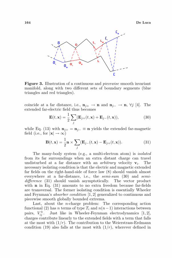
An invariant manifold M of the variational two-body problem is apair of continuous and piecewise smooth trajectories such that for anypair of boundary segments in M, the extremum of the correspondingboundary-value problem is a segment of M, as illustrated in Fig. 3.Unlike the case of an ODE, trajectories of M can have corners and onecan not continue trajectories with a time integration (neither forwardnor backwards). The infinite-dimensional problem at hand is to find awhole function, just like solving a partial differential equation (PDE)with boundary conditions.

For a many-body system, physically interesting are globallybounded invariant manifolds. Given that all trajectories are spatiallybounded, one can show that all advanced and retarded normals

164 De Luca

O+

OL-

L+

L

O-

O

O-

O+

L

L-

L+

Figure 3. Illustration of a continuous and piecewise smooth invariantmanifold, along with two different sets of boundary segments (bluetriangles and red triangles).

coincide at a far distance, i.e., nj+ → n and nj− → n, ∀j [4]. Theextended far-electric field thus becomes

E(t,x) =12

∑

j

(Ej+(t,x) + Ej−(t,x)), (30)

while Eq. (13) with nj+ = nj− ≡ n yields the extended far-magneticfield (i.e., for |x| → ∞)

B(t,x) =12n×

∑

j

(Ej−(t,x)−Ej+(t,x)). (31)

The many-body system (e.g., a multi-electron atom) is isolatedfrom its far surroundings when an extra distant charge can travelundisturbed at a far distance with an arbitrary velocity vi. Thenecessary isolating condition is that the electric and magnetic extendedfar fields on the right-hand-side of force law (8) should vanish almosteverywhere at a far-distance, i.e., the semi-sum (30) and semi-difference (31) should vanish asymptotically. The vector productwith n in Eq. (31) amounts to no extra freedom because far-fieldsare transversal. The former isolating condition is essentially Wheelerand Feynman’s absorber condition [1, 2] generalized to continuous andpiecewise smooth globally bounded extrema.

Last, about the n-charge problem: The corresponding actionfunctional (2) has n terms of type Ti and n(n−1) interactions betweenpairs, V ±

ij . Just like in Wheeler-Feynman electrodynamics [1, 2],charges contribute linearly to the extended fields with a term that fallsat the most with (1/r). The contribution to the Weierstrass-Erdmanncondition (19) also falls at the most with (1/r), wherever defined in


space-time. It is therefore a good approximation to disregard universalperturbations of distant charges.

5. CIRCULAR ORBITS

The electromagnetic two-body problem has globally defined circularorbit solutions [20]. The stability of circular orbits is studied in [21–23] and the quantization of circular orbits is discussed in [24, 25].Circular orbits with large radii are discussed below using the notationof Ref. [23].

The constant angular velocity and distance in light-cone aredenoted by Ω and rb, respectively, and the angle θ ≡ Ωrb that particlesturn in the light-cone time is henceforth called the delay angle. Thefamily of subluminal circular orbits [20] is parametrized by θ, and forquantum Bohr orbits it turns out that θ . 10−2 [26, 27]. Along orbits ofa small delay angle the Kepler formulas yield the leading order angularvelocity and distance in light-cone, respectively

Ω = µθ3 + O(θ5), (32)

rb =θ

Ω=

1µθ2

, (33)

where reduced mass and total mass are defined by µ ≡ m1m2/M andM ≡ m1 + m2. It is important to keep these limiting dependenciesin mind, and for hydrogen µ ' (1836/1837) ' 1. Adopting the samenotation of Ref. [23], we express each particle’s circular orbit’s radiusby numbers 0 ≤ bi < 1 as

ri ≡ birb, (34)

which define scalar velocities

vi = Ωri = θbi, (35)

for i = 1, 2.The speed of light limit c ≡ 1 imposes that max(θb1, θb2) ≤ 1.

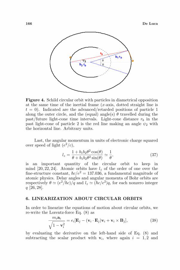
In the limit of a small mass-ratio, (µ/M) → 0, one has θ ∈ (0, 1],the upper limit θ = 1 corresponding to the particle of smaller mass(m1) traveling at the speed of light. As illustrated in Fig. 4 andin Ref. [20], the circular radii and the distance in light-cone form atriangle of largest side rb, yielding a trigonometric constraint

b21 + b2

2 + 2b1b2 cos(θ) = 1, (36)

equivalent to Eq. (31) of Ref. [20]. Using the ratio of Eqs. (32) and (33)of Ref. [20] to eliminate Ω, together with constraint (36), we find thesolution b1 = (1 + µθ2

2M )m2M + O(θ4) and b2 = (1 + µθ2

2M )m1M + O(θ4).

166 De Luca

b1

rb

b2 r

b

rb

2Ψ θ

θ

Figure 4. Schild circular orbit with particles in diametrical oppositionat the same time of the inertial frame (x-axis, dotted straight line ist = 0). Indicated are the advanced/retarded positions of particle 1along the outer circle, and the (equal) angle(s) θ travelled during thepast/future light-cone time intervals. Light-cone distance rb in thepast light-cone of particle 2 is the red line making an angle ψ2 withthe horizontal line. Arbitrary units.

Last, the angular momentum in units of electronic charge squaredover speed of light (e2/c),

lz =1 + b1b2θ

2 cos(θ)θ + b1b2θ2 sin(θ)

' 1θ, (37)

is an important quantity of the circular orbit to keep inmind [20, 22, 24]. Atomic orbits have lz of the order of one over thefine-structure constant, ~c/e2 = 137.036, a fundamental magnitude ofatomic physics. Delay angles and angular momenta of Bohr orbits arerespectively θ ' (e2/~c)/q and lz ' (~c/e2)q, for each nonzero integerq [26, 28].

6. LINEARIZATION ABOUT CIRCULAR ORBITS

In order to linearize the equations of motion about circular orbits, were-write the Lorentz-force Eq. (8) as

miai√1− v2

i

= ei[Ej − (vi ·Ej)vi + vi ×Bj ], (38)

by evaluating the derivative on the left-hand side of Eq. (8) andsubtracting the scalar product with vi, where again i = 1, 2 and


j ≡ 3− i. The magnetic term (last term on the right-hand side of (38))is a transversal force proportional to the electric field by (13), andfurther proportional to the velocity modulus |vi|, which is small forsmall θ (see Eq. (35)).

For small delay angles, the electric force, first term on the right-hand-side of Eq. (38), is responsible for the significant contributions tothe linearized equations along a circular orbit. The electric field (11)of charge j ≡ 3 − i acting on charge i decomposes in two terms: (i)the near-electric field proportional to 1/r2

j±, a magnitude of µ2θ4 byuse of (33), times a unit vector (almost) along the particle separationat the same time, n(t); and (ii) the far-electric field proportional to1/rj±, a magnitude of µθ2 by use of (33), times a vector along thecircular orbit.

It is important to ponder upon the magnitude of each electriccontribution: the far-electric field is almost transversal to the particleseparation at the same time, n(t), such that projection along n(t)involves the (small) factor of cos(−θ + π/2) ' θ. Separating thecontributions of near-fields and far-fields, the right-hand-side of (38)has the combined magnitude

Fi ∝ O(θ4) + |aj |O(θ3). (39)

In Eq. (39), the near-field contribution is O(θ4) while the far-fieldcontribution is |aj |O(θ3), which is smaller along circular orbits since|aj | ∝ 1/r2

b = O(θ4). The force along circular orbits is approximatelydescribed by the near field only because the far-field (11) is furtherproportional to the O(θ4) acceleration of circular orbits. Uponlinearization about the circular orbit, this dominance changes: thelinearized equations accept solutions of arbitrarily large accelerations,and the most important contribution to the linearized version ofEq. (38) is precisely the contribution of the far-field term.

Next we derive the linearized equations along the orbital planeusing the notation of Ref. [23]. We introduce complex gyroscopiccoordinates where the circular orbit is a fixed point of the equations ofmotion, i.e.,

xj + iyj ≡ rb exp(−iΩt)[bj + lj + iuj ], (40)

where (lj , uj) are respectively the longitudinal and transversalgyroscopic coordinates. The circular orbit [20] is the fixed point(lj , uj) = (0, 0) for j = 1, 2. Again, while small-delay-angle circularorbits have O(θ4) accelerations, the linearized acceleration corrections,δaj , can be arbitrarily large [23]. The dominant linear correctionfor the accelerations (the stiff limit of Ref. [23]) is obtained using(38) with only the first term on the right-hand side and far-field Ej±

168 De Luca

approximated by

Ej± ' 1rb

nj± × (nj± × δaj±) =1rb

(nj± · δaj±)nj± − 1rb

δaj±, (41)

where ± indicate evaluation at the unperturbed deviating timest ± (θ/Ω) (because we want the linear term only). The gyroscopicrepresentation of the rotating normals in light-cone are complexnumbers of unit modulus, i.e., exp(−iΩt) exp(iψj), where

exp(iψ1) ≡ b1 + b2 exp (iθ),exp(iψ2) ≡ b2 + b1 exp (iθ). (42)

Equation (36) can be used to show that the modulus of each complexnumber on the right-hand-side of (42) is unitary. Angles ψ1 and ψ2

further satisfy ψ1 +ψ2 = θ, and for small θ the bi given below Eq. (36)yield ψ1 ' m1

M θ and ψ2 ' m2M θ. In Fig. 4, ψ2 is the angle between the

(rotating) red line and the x-axis (dashed line).The linearized planar equations of motion are obtained substitut-

ing (40) into (38) with only its first right-hand-side term given by thesemi-sum of retarded and advanced fields (41). The real and complexparts of the linearized equations of motion keeping only the largestderivatives of the gyroscopic coordinates yields

m1rb l1 = −C11

(l2+ + l2−

)

2− S11

(u2+ − u2−)2

,

m2rb l2 = −C21

(l1+ + l1−

)

2− S21

(u1+ − u1−)2

,

m1rbu1 = −C31(u2+ + u2−)

2− S31

(l2+ − l2−

)

2,

m2rbu2 = −C41(u1+ + u1−)

2− S41

(l1+ − l1−

)

2,

(43)

where Cj1 and Sj1 are 4× 1 matrices defined by

C ≡ −

cos θ − cosψ2 cos θcos θ − cosψ1 cos θcos θ + sinψ2 sin θcos θ + sinψ1 sin θ

≡ (coshλ)−1D, (44)

and

S ≡ −

sin θ − sinψ2 cos θsin θ − sinψ1 cos θ(1− cosψ2) sin θ(1− cosψ1) sin θ

≡ (sinhλ)−1E. (45)


In Eqs. (44) and (45), 4× 1 matrices D and E are defined to be usedbelow.

Equation (43) is a linear NDDE with exponential solutions

lj = Lj exp(λΩt/θ),uj = Uj exp(λΩt/θ), (46)

where j = 1, 2 and (L1, L2, U1, U2) is a non-trivial solution of

m1rb D11 0 E11

D12 m2rb E12 00 E13 m1rb D13

E14 0 D14 m2rb

L1

L2

U1

U2

= 0. (47)

A nontrivial solution of Eq. (47) requires the vanishing of its 4×4determinant,

Fxy = 1− µθ4

Mcosh2(λ) = 0, (48)

where powers of θ2 coshλ with coefficients of O(θ4) were discarded,henceforth and in Ref. [23] called the stiff-limit. The roots of Eq. (48)exist in symplectic sets of four, i.e., (λ,−λ, λ∗,−λ∗). For atomichydrogen, θ−1 ∼ 137.036 and (µ/M) ' (1/1836), such that Eq. (48)requires λ to have a positive real part |<(λ)| ≡ σ = ln(

√4Mµθ4 ) ' 14.29.

The imaginary part of λ is any integer multiple of πi. The generalsolution of Eq. (48) modulo the symplectic symmetry is

λ = σ + πqi, (49)

where i ≡ √−1 and q ∈ Z.Solution (49) was called a ping-pong mode in Ref. [23] because

its phase advances by πq in one light-cone time rb, a phase speed ofπqΩ/θ = µθ2πq = πq/rb = (Ω/θ)=(λ). The only O(1) off-diagonalterms of matrix (47) are D13 and D14, others being O(θ) or higherorder. The nontrivial eigenvector solution is approximately

(L1, L2, U1, U2) ∝(

µθ

M,µθ

M, 1,

√µ

M

). (50)

For m2 À m1, normal-mode solution (46) oscillates (almost) alongthe circular orbit because Eq. (50) yields Ui À Li, thus defining aquasi-transversal mode. The largest longitudinal component, Li, isattained for positronium at moderate θ. Solution (49) defines a nonzeroreal part for λ that causes amplitudes to blow up at either t → ±∞,implying that besides the Schild circular orbits [20], no other near-circular orbit can be simultaneously C2 and globally bounded.

170 De Luca

The inclusion of O(1/λ) and O(1/λ2) linear terms to the planarmotion is outlined in Ref. [23]. The linearized motion perpendicularto the orbital plane is studied analogously. As explained in [23], thez-oscillations are transversal modes that decouple from the planartransversal oscillations (43) at linear order. The determinant of thelinearized 2×2 system in the limit |λ| → ∞ is again (48), an asymptoticdegeneracy. The degeneracy is raised by O(1/λ2) corrections to (47)and (48) introduced by the linear terms with lower derivatives [23].

The determinant for planar modes is calculated in Ref. [23] up toO( 1

λ4 ) terms (see Eq. (41) of Ref. [23] with Γ = −1/2), i.e.,

Fxy = 1− µθ4

M

(1 +

7λ2

+5λ4

)cosh2(λ)

+µθ4

M

(1λ

+5λ3

)sinh(2λ) = 0, (51)

where we have disregarded O( θ2

λ2 ) terms not proportional to the largehyperbolic functions. The determinant for perpendicular oscillationsand up to O( 1

λ4 ) terms is Eq. (B17) of Appendix B in Ref. [23] withΓ = −1/2, i.e.,

Fz = 1− µθ4

M

(1− 1

λ2+

1λ4

)cosh2(λ)

+µθ4

M

(1λ− 1

λ3

)sinh(2λ) = 0, (52)

again disregarding O(θ2) terms that are not multiplied by the largehyperbolic functions. Notice the symplectic symmetry that roots ofEqs. (51) and (52) are still in sets of four, (λ,−λ, λ∗,−λ∗). The firstcorrection at O( 1

λ) is the same for the roots of both of Eqs. (51)and (52). The corrections at O( 1

λ2 ) separate Eq. (51) from (52),unfolding the asymptotic degeneracy of planar and perpendiculartransversal modes at |λ| → ∞.

7. BOUNDARY LAYER

Atomic gases containing Avogadro’s number of atoms pose a many-body problem where each atom suffers perturbations from all otheratoms. In the following we attempt to validate our theory byexploring an isolating mechanism to allow a sensible modelling ofnature. Electromagnetic isolation requires globally bounded orbitswith vanishing far fields, in order to decouple individual atoms fromexperimental boundaries and/or other atoms. Circular orbits are


not good candidates because these create non-vanishing far-fields.In Ref. [4] it is shown that globally bounded two-body orbits withvanishing far-fields must involve velocity discontinuities.

The non-zero real part of growth-rate Eq. (49) suggests that thereare no other near-circular C2 solutions besides circular orbits, and thelinearized modes blow up at either t → ±∞. This unless a cornerpoint invalidates the linearization. Therefore, we are led again to seekglobally bounded extrema with corner points.

Figure 5 illustrates a pair of boundary segments containingboundary-layer regions of fast motion along the light-cone separation,segments abc and fed, henceforth spikes. As explained in Ref. [8],a neutral differential delay equation (NDDE) can propagate thediscontinuity to the next segment (see method of steps and examplesof NDDE’s versus ODE’s in Ref. [8]). In other words, spikes along theorbit are created by spikes inside the boundary segments illustrated inred in Fig. 5.

ac

h

gd f

b

e

d

Figure 5. Illustrated are (i) elsewhere boundary segment (red) ofparticle 1 with a spike along the advanced light-cone (ab) to cornerpoint (b); and (ii) elsewhere boundary segment 2 with a spike to cornerpoint (e) (red line). At points (a) and (c), perturbed orbit 1 (redand blue solid lines) have a corner to/from the 180-degree corners (b)and (e). Boundary layer magnitudes are exaggerated for illustrativepurposes. Arbitrary units.

We set about the task to construct a periodic broken extremumusing a boundary-layer perturbation that assumes regular segmentsseparated by boundary layer regions (spiky segments) each containingone or more corner points, as illustrated in Fig. 5. Along bothtrajectories, boundary layers have an angular width αθ ¿ θ. Outsideboundary layers we can linearize because trajectories are C2 and

172 De Luca

deviating arguments fall on C2 segments as well. Inside boundarylayers we do not linearize but rather use a variational approximationusing head-on collisional trajectory segments, and apply the necessarycondition (19) at rebouncing corners.

The roots of Eqs. (51) and (52) near each root (49) of the limitingEq. (48) are, respectively,

λxy(θ, q) ≡ σxy + πqi + iεxy, (53)λz(θ, q) ≡ σz + πqi + iεz, (54)

where q is an arbitrary integer, εxy(θ, q) = −εxy(θ,−q) andεz(θ, q) = −εz(θ,−q) (by the symplectic symmetry). An O(µθ4/M)approximation for positive σ is obtained by setting 4 cosh2(λ) ≈2 sinh(2λ) ≈ exp(2λ) into Eqs. (51) and (52), thus defining polynomials

Fxy(λ) = 1− µθ4

4Mexp(2λ)

(1− 2

λ+

7λ2− 10

λ3+

5λ4

)

≡ 1− µθ4

4Mexp(2λ)pxy

(1λ

)= 0, (55)

and

Fz(λ) = 1− µθ4

4Mexp(2λ)

(1− 2

λ− 1

λ2+

2λ3

+1λ4

)

≡ 1− µθ4

4Mexp(2λ)pz

(1λ

)= 0. (56)

It follows from Eqs. (51) and (53) that

exp(4iεxy) =pxy( 1

λ∗xy)

pxy

(1

λxy

) , (57)

while Eqs. (52) and (54) yield

exp(4iεz) =pz( 1

λ∗z)

pz( 1λz

). (58)

Disregarding the contribution of εxy and εz and replacing λxy =λz = σ + πqi into the right-hand-sides of (57) and (58) yields, to thefirst order in (1/λ)

εxy ' εz = =(

1λ

)=

−πq

(σ2 + π2q2). (59)

We henceforth use a positive integer q, so that the energetic mismatchesεxy and εz predicted by Eq. (59) are negative O( 1

λ) numbers.


Another order can be gained expanding the right-hand-side of (57)in a Taylor series on the deviation εxy about λq = σ + πqi, whichgenerates only terms at O(1/λ3), so that up to O(1/λ2) Eq. (57) yields

εxy(q) =−πq

(σ2 + π2q2)+

5πqσ

(σ2 + π2q2)2, (60)

εxy negative and monotonically increasing for q ≥ 6. Analogously,the right-hand-side of (58) evaluated at λq = σ + πqi yields εz up toO(1/λ2)

εz(q) =−πq

(σ2 + π2q2)− 3πqσ

(σ2 + π2q2)2, (61)

again negative and monotonically increasing for q ≥ 6.Let us assume a corner along orbit 1 at t = 0, illustrated by the

dashed line in Fig. 5. We define the first regular layer αrb < t < rb−αrb

as the first and last zeros of the (exponentially increasing and fastoscillating) perturbation inside the first light-cone time zone. Usinga linear combination of the symplectic quartet of linearized modes,and (40) and (50) with l1 ∝ L1 = µθ

M and u1 ∝ U1 = 1, the orbitalperturbation constructed to vanish at layer edges is

(δxj

δyj

)=

(µθAMA

) cosh(σxytrb

)

cosh(σxy

2 )sin

([πq + εxy(q)− θ](t− αrb)

rb

). (62)

From (a) to (h) the velocity of the perturbed orbits oscillate fast,and at points (a) and (h) the perturbation of trajectory 1 crosses theunperturbed orbit 1 (the perturbations are not illustrated in Fig. 5).In Eq. (62), σxy and εxy are given by (53) and we must have A < rb

πq , toavoid a superluminal velocity at layer edges. Along the regular regionthe phase of the sine function in (62) advances by almost πq, and thecondition of vanishing at t = rb − αrb yields α = (εxy−θ)

2πq .The variational approximation for the boundary-layer motion is

illustrated in Fig. 5, with corners along a given orbit all equivalentby a θ-rotation. The central spike starts along trajectory 1 with aninety-degree corner, point (a), and respective corner in light-conealong trajectory 2, point (d). Next is a straight-line segment of acollisional trajectory (ab) terminated by an almost 180-degree corner((b) and (e)), then a straight-line climb (bc) to the last ninety-degreecorner ((c) and (f)), resuming motion along the next regular layer.

Corners are nontrivial solutions of condition (19), and 180-degreecorners, (points (b) and (e) in Fig. 5), are simpler to analyse:for a nontrivial corner, condition (19) requires the other particleto have a velocity discontinuity at least at one of the light-cones.

174 De Luca

For simplification, we study resonant minimizers where velocities arediscontinuous at both light-cones and further specialized to 180-degreecorners that are spikes along the local radial direction ρj to eachcircular orbit, ρj± · vl

j± = −ρj± · vrj±. Moreover, we consider only

periodic minimizers such that all corners are equivalent by a rotationof θ, i.e., satisfy the discrete-rotation-symmetry nj+ · vl

j+ = nj− · vlj−

and nj+ · vrj+ = nj− · vr

j−.For planar motion, condition (19) yields four equations, one along

each Cartesian direction and for i = 1, 2. For the assumed radialspikes the vectorial components of (19) perpendicular to each ρi vanish,yielding a 2× 2 linear homogeneous system for the ρj ·∆vj = 2|vj |,(

(E1 + 1rD2

) − cos θrD2

− cos θrD1

(E2 + 1rD1

)

)(|v1||v2|

)= 0. (63)

The vanishing determinant of a nontrivial solution to Eq. (63) in thelimit cos(θ) → 1 can be expressed as

Det = E1E2 +1r(E1

D1+

E2

D2) = 0, (64)

where D1 ≡ (1− (n1 · v1)2) and D2 ≡ (1− (n2 · v2)2) are evaluated atthe corner and r is the distance from point (b) to point (e) in Fig. 5.Since the Di are positive, inspection of (64) shows that at least oneenergy must be negative for a nontrivial solution.

The energies defined by (18) for radial spikes at large separationsare the following functions of time

E1 =m1√1− v2

1

− 1rD2

, (65)

E2 =m2√1− v2

2

− 1rD1

. (66)

Nonlinear Eqs. (64), (65) and (66) can be solved for r, yielding

r2 =1

m1m2

√1− v2

1

D1

√1− v2

2

D2

=1

m1m2

√1− v2

1

(1− (n1 · v1)2)

√1− v2

2

(1− (n2 · v2)2), (67)

proving that a separation in light-cone r of the order of the (large)circular radius rb = 1/µθ2 requires that |nj · vj | → 1 at least for oneparticle, which in turn requires a quasi-luminal velocity. Again, partialenergies are not constants of motion and may assume the needed spiky


negative values only for a split second during the boundary-layer time(the exponential blow-up time is Ω

2πrbσ ' θ

2πσ circular periods).Assuming m2 À m1 = 1, and a trajectory with a large separation

rb = 1/µθ2, if r in Eq. (67) is to be near the large circular radiusr1 ≈ rb = 1

µθ2 of trajectory 1, then the (ab) straight-line spiky segmentof Fig. 5 must be (almost) along the light-cone direction such thatD1 ≡ (1 − (n1 · v1)2) can be small at the corner and the value of E2

negative (possibly negative only for the split second of the spike). Theformer conditions are achieved simply by letting the electron have alarge radial velocity at point (b) of Fig. 5.

Notice that (67) solves the fully nonlinear condition (19) withoutany approximation; the 180-degree corners function as stepping-stoneswhen one particle reaches the critical quasi-luminal velocity necessaryfor the formation of corners at-a-far-distance. Corner creation at a fardistance is a rebouncing mechanism alternative to charges falling intoeach other.

Last, we discuss if and how ninety-degree corners satisfy theextremum condition, to complete the justification of the minimizerof Fig. 5 (points (a) and (c) in Fig. 5). We recall thatperturbation (62) naturally blows up after each one-light-cone time,generating synchronized and periodic velocity bursts lasting for thevery small boundary-layer times, enough to trigger the spikes. Theratio of the small boundary-layer time to the period is a good estimateof the (small) probability of finding a large velocity.

For the most general co-planar corner problem, condition (19)yields a 4× 4 homogeneous system with linear matrix having diagonalelements equal to Ei plus terms of the order of 1/(rDj), while theoff-diagonal terms are proportional to 1/(rDi), a generic form sharedby matrix (63). Again, the fully nonlinear necessary condition fora 90-degree turn at large separations is the vanishing of the 4 × 4determinant, which requires the vanishing of one of the Ei, which inturn requires a large denominator and a quasi-luminal velocity. Acondition analogous to (67) results from a fully nonlinear analysis ifvelocities are to increase along the circular orbit right before corner(a) of Fig. 5. Again, the exponential blow-up of Eq. (62) eventuallyreaches that necessary quasi-luminal velocity at layer edge if A ' rb

πq .The physical intuition about the spikes of Fig. 5 is that the

synchronised velocity bursts create large-amplitude electromagneticfields at the other particle. These fields represent photons carryingmomentum along the direction n of particle separation, and themechanism of continuous absorption of momentum from transversalelectromagnetic waves is discussed in textbooks [6]. What is necessaryto explain within variational electrodynamics is the mechanism

176 De Luca

to switch from the circular trajectory to a quasi-luminal head-oncollisional trajectory at a discontinuous rate above threshold, a collapsecaused by the bursting attractions between particles. At a far-distance the spiky behaviour goes unnoticed because the synchronisedlongitudinal chase has a vanishing net current and produces weak Biot-Savart fields.

Weierstrass-Erdmann conditions were used in Ref. [29] to modeldouble-slit interference caused by interaction-at-a-distance with thevelocity discontinuities of the bounded trajectories of material electronsinside the grating. Our Eqs. (16) and (18) are exactly Eqs. (16)and (17) of Ref. [29], while the above explained criteria provided bythe vanishing of the partial energies is the content of Eqs. (19) and (20)of Ref. [29].

8. FINITELY MEASURED NEIGHBOURHOOD OFBROKEN MINIMIZERS

The tangent dynamics of circular orbits has an infinite number ofunstable transversal modes of arbitrarily large frequencies, as seenby the linear growth frequencies (53) and (54). This is unlike theclassical Kepler problem, whose tangent dynamics has a finite numberof frequencies of the order of the orbital frequency [31, 32]. Sincelinearized modes (53) and (54) are unstable, continuation along theC2 segment would blow up, and a velocity discontinuity is neededto break away from the C2 segment. A corner requires stepping-stone condition (64), and for a small neighbourhood of minimizerswith corners to exist, circular orbits with planar and perpendicularperturbations require the resonances studied below.

The perpendicular perturbation in the regular region is con-structed analogously to the planar perturbation (62), using the lin-earized modes explained in Appendix B of Ref. [23], yielding

δzj = Bcosh(σz

rbt)

cosh(σz2 )

sin(

[πs + εz(s)](t− αrb)rb

), (68)

where s is any integer (possibly different from q) and B is an arbitraryamplitude smaller than rb

πs to avoid a superluminal velocity at layeredge. Again, the amplitude of the transversal perturbation (68) isconstructed to vanish along the circular orbit at both edges t = αrb

and t = rb − αrb, to keep the property that corners see other cornersin light-cone (a boundary-layer-adjusted resonance).

Since the phase of oscillation (' πs/rb) is fast, a large orbitalvelocity at layer edge results from a small amplitude B ' rb

πs , which isillustrated in Fig. 5. Layer edge amplitudes of both types of transversal


modes should vanish while their derivatives reach a quasi-luminalvelocity. Amplitude (62) vanishes at t = rb − αrb if

[πq + εxy(q)− θ](1− 2α) = πq, (69)

other multiples of π being excluded because εxy(q), θ and α are small.Analogously, amplitude (68) vanishes at t = rb − αrb if

[πs + εz(s)](1− 2α) = πs, (70)

where again other integer multiples of π are impossible because εz(s)and α are small.

If Eqs. (69) and (70) hold, both edges t = αrb and t = rb−αrb havethe same quasi-luminal |vj | for arbitrary amplitudes near (A,B) =( rb

πq , rbπs). For this it is necessary that

θ =qεxy(q)− sεz(s)

q, (71)

as obtained eliminating α from Eqs. (69) and (70). If condition (19)holds at corner (c) of Fig. 5, then by Eq. (71) it automatically holdsat corner (a) of Fig. 5, which carries on to all other corners by thediscrete θ rotational symmetry. Condition (71) is also a probabilisticcondition, i.e., given (71) a whole neighbourhood of orbits with (A,B)near ( rb

πq , rbπs) is focused like a caustic into the Kernel of the corner point,

thus allowing a finitely measured neighbourhood of broken extrema.Figure 6 illustrates the exponentially exploding transversal

perturbations (68) and (62) being focused into the corners at bothlayer edges. The perturbations need to be in phase to be focused in andout of both corners with the same large velocity amplitude required byEq. (19) for the 90-degree turn at edges, which imposes resonance (71),henceforth the external resonance. Condition (19) yields a vanishingdeterminant with a nontrivial null-vector generating a linear space(Kernel), which freedom that can be used to make (19) hold alongslightly different orbits, thus generating periodic orbits passing byevery point inside a finite volume around the resonant orbit.

Next we calculate the magnitudes of the finitely measuredminimizers with q = s. For each q = s, condition (71) determinesa unique θ together with Eqs. (51) and (52), as listed in Table 1. Forcomparison, Table 1 also lists the first line of each spectroscopic series,i.e., the circular lines from quantum level k + 1 to quantum level k.Historically, the series of hydrogen were named after Lyman, Balmer,Ritz-Paschen, Brackett, etc.. The frequency over reduced mass of thefirst line of each spectroscopic series in atomic units is the secondcolumn of Table 1. We used a Newton method in the complex-λ planeto solve Eqs. (51), (52) and (71), as used in Ref. [23] with Dirac’s

178 De Luca

δz

δφCaustic focuses

Figure 6. The angular perturbation δφ along the circular orbitis illustrated by the green line. Illustrated is also the transversalperturbation δz (brown). The resonant caustic focus is created whenδφ and δz perturbations vanish at both ends of each regular segment,by resonance condition (71). Arbitrary units.

theory. Our calculations for hydrogen used the protonic-to-electronicmass ratio (m2/m1) = 1836.1526. Table 1 gives frequency over reducedmass calculated by QM for the first line of the kth spectroscopic series(atomic units), numerically calculated orbital frequency over reducedmass (for a suitable integer q(k)), (1373Ω)/µ = 1373θ2(εxy − εz),angular momentum of unperturbed circular guide, and integer q.

Table 1 is to be compared with Table 1 of Ref. [23], which discussesDirac’s electrodynamics with self-interaction. The same surprisingagreement is found in Ref. [23]. Notice that we also skipped theq = 10 value in Ref. [23], again because the resonance condition isonly necessary.

As mentioned below Eqs. (60) and (61), the energetic mismatchesare monotonically increasing for q ≥ 6, and the frequencies of Table 1agree within ten percent with the first twelve circular hydrogen linesstarting from q = 7 at k = 1, i.e., q(1) = 7. Since condition (71) isonly necessary (and not sufficient), some values of q may correspondto unstable orbits. This is analogous to the description by QM [27],where there are selection rules on top of three conditions involvinginteger quantum numbers, and Table 2 includes the lines that wereskipped in Table 1. A theory for the q’s that were skipped is presentlylacking. Inspection of Table 2 shows that for q = 1, 2, 3, 4, 5, 6 condition(71) predicts θ still in the atomic range, but the angular momentumspacing is about half of Planck’s constant. Table 2 also includes theskipped numerical calculations for q = 8 and q = 10.


Table 1. Numerical calculations for hydrogen with (m2/m1) =1836.1526. Quantum number k of the circular Bohr transition k+1 →k, frequency over reduced mass of the circular QM line in atomic units,wQM ≡ 1

2( 1k2 − 1

(k+1)2), orbital frequency over reduced mass in atomic

units, (Ω/µ) = 1373θ2(εxy − εz), angular momentum of unperturbedorbit in units of e2/c, lz = θ−1, and integer q.

k wQM 1373θ2(εxy − εz) lz = θ−1 q

1 3.750×10−1 3.852×10−1 188.32 72 6.944×10−2 8.919×10−2 306.67 93 2.430×10−2 2.485×10−2 469.54 114 1.125×10−2 1.392×10−2 569.61 125 6.111×10−3 8.070×10−3 683.13 136 3.685×10−3 4.825×10−3 810.89 147 2.406×10−3 2.966×10−3 953.65 158 1.640×10−3 1.870×10−3 1112.21 169 1.173×10−3 1.206×10−3 1287.27 1710 8.678×10−4 7.942×10−4 1479.62 1811 6.600×10−4 5.329×10−4 1690.02 1912 5.136×10−4 3.639×10−4 1919.20 20

Analogy with Sommerfeld’s quantization suggests there must bethree conditions like (71), involving three integer quantum indices,reinforcing that our single condition (71) is only necessary and alonemight not determine a stable orbit. Inspection shows that if the valuesof Table 2 were included in Table 1, the angular momentum jump fromconsecutive lines would be much lesser than about a hundred units ofe2/c, which is suggestive of what the missing conditions should do.

In Table 3 we give the numerical calculations for muonium usingthe positive-muon-to-electron mass ratio (m2/m1) = 1836.1526/9.Table 3 lists the frequency over reduced mass of the first line ofeach spectroscopic series as calculated with QM (in atomic units),orbital frequency in atomic units, (1373Ω)/µ = 1373θ2(εxy − εz), andangular momentum of unperturbed circular orbit in units of e2/c. Theagreement of the numerical calculations with the atomic magnitudesand QM is again within a few percent for frequencies.

Last, Table 4 gives the numerical calculations for positroniumusing the positron-to-electron mass ratio (m2/m1) = 1: Table 4 liststhe frequency over reduced mass of the first line of each spectroscopic

180 De Luca

Table 2. Numerical calculations for hydrogen with q < 7 and(m2/m1) = 1836.1526. Orbital frequency over reduced mass in atomicunits, (Ω/µ) = 1373θ2(εxy − εz), angular momentum of unperturbedcircular guide in units of e2/c, lz = θ−1, and integer q.

1373θ2(εxy − εz) lz = θ−1 q

1.506 119.53 110.653 62.27 29.466 64.77 34.664 82.01 42.006 108.63 5

8.622×10−1 143.96 61.808×10−1 242.32 8

4.6095 ×10−1 382.16 10

Table 3. Numerical calculations for muonium with (m2/m1) =1836.1526/9. Quantum number k of the circular Bohr transitionk + 1 → k, frequency over reduced mass of the circular QM line inatomic units, wQM ≡ 1

2( 1k2 − 1

(k+1)2), orbital frequency over reduced

mass in atomic units, (Ω/µ) = 1373θ2(εxy− εz), angular momentum ofunperturbed circular guide in units of e2/c, lz = θ−1, and integer q.


1 3.750×10−1 4.039×10−1 185.63 72 6.944×10−2 8.762×10−2 308.94 93 2.430×10−2 2.356×10−2 478.65 114 1.125×10−2 1.304×10−2 582.96 125 6.111×10−3 7.491×10−3 701.31 136 3.685×10−3 4.445×10−3 834.53 147 2.406×10−3 2.717×10−3 983.41 158 1.640×10−3 1.704×10−3 1148.75 169 1.173×10−3 1.095×10−3 1331.34 1710 8.678×10−4 7.187×10−4 1531.19 1811 6.600×10−4 4.810×10−4 1751.36 1912 5.136×10−4 3.277×10−4 1990.34 20


Table 4. Numerical calculations for positronium with (m2/m1) = 1.Quantum number k of the circular Bohr transition k + 1 → k,frequency over reduced mass of the circular QM line in atomic units,wQM ≡ 1

2( 1k2 − 1

(k+1)2), orbital frequency over reduced mass in atomic

units, (Ω/µ) = 1373θ2(εxy − εz), angular momentum of unperturbedorbit in units of e2/c, lz = θ−1, and integer q.


1 3.750×10−1 3.423×10−1 246.76 82 6.944×10−2 7.749×10−2 404.86 103 2.430×10−2 2.189×10−2 617.037 124 1.125×10−2 1.240×10−2 745.61 135 6.111×10−3 7.286×10−3 890.33 146 3.685×10−3 4.416×10−3 1052.06 157 2.406×10−3 2.753×10−3 1231.64 168 1.640×10−3 1.759×10−3 1429.92 179 1.173×10−3 1.149×10−3 1647.73 1810 8.678×10−4 7.667×10−4 1885.88 1911 6.600×10−4 5.209×10−4 2145.20 2012 5.136×10−4 3.599×10−4 2426.50 21

series calculated by QM (in atomic units), orbital frequency overreduced mass in atomic units, and the angular momentum of theunperturbed circular orbit in units of e2/c.

Notice in Table 4 that for positronium the values of lz = 1/θare consistently larger. Using again the fact that condition (71) isonly necessary, Table 4 starts the q, when the angular momentumspacing is about constant, i.e., at q = 8. For positronium the numericalcalculations find the first root 1/θ = 40.501 only at q = 3, again in theatomic magnitude. The spectrum agrees with QM within less than afew percent for the circular lines of the first 12 series.

In the days of Bohr, only twelve lines of the Balmer series couldbe observed with vacuum tubes, and about thirty-three from celestialspectra [26].

Surprizingly, the emission frequencies agree better with QM forthe decays from the twelve deepest quantum levels. As explainedin [23], the cancelation of dipolar far-fields involves quadratic termsthat might require larger amplitudes at large q. Given that the xy

182 De Luca

modes modify the unperturbed z-angular momentum more and moreat larger q, our perturbative results should get worse at larger q.

We have carried the numerical calculations up to q = 43 (notshown in Table 2) and observed that the angular momentum spacingincreases slowly with q. The agreement of the numerical calculationswith an effective angular momentum separation seems to continuewithin thirty percent, suggesting that one can approximate a largenumber of eigenvalues near the discrete spectrum of Schroedinger’sequation.

The agreement with emission lines for k > 13 slowly deteriorates,suggesting that the corresponding minimizers are becoming far fromplanar. A one-to-one comparison with natural spectra should waitthe investigation of broken extrema with spikes filling a tridimensionalregion.

The surprising agreement of the numerical calculations with auniversal value for the fine-structure constant is due to the logarithmicdependence of σ(θ) ≡ ln(

√4Mµθ4 ) on (µ/M), as explained above Eq. (49).

Formulas (60) and (61) yield an implicit equation for θ, i.e.,

1θ

=1

εxy − εz=

(σ2(θ) + π2q2)2

8πqσ(θ). (72)

The roots of (72) are insensitive to changes in (µ/M) over three ordersof magnitude, e.g., for q = 7 and (µ/M) = 1/1837 (hydrogen), Eq. (72)yields θ ' 190.09, while for q = 7 and (µ/M) = 9/1836 (muonium),Eq. (72) yields θ ' 187.17, and last for q = 7 and (µ/M) = 1/4(positronium), Eq. (72) yields θ ' 186.81. The numerically calculatedvalues of lz ≡ θ−1 fall approximately between the consecutive Bohrorbits k and k + 1. Tables 1, 3 and 4 show that frequencies of spectrallines agree even better with the spectroscopic series.

Notice that the orbital frequencies determined by (71) areexpressed as a difference of two spectroscopic terms, just like theRydberg-Ritz principle of atomic physics, i.e.,

Ω ≡ µθ3 = (µθεxy(q)− µθεz(s)) /(1/θ), (73)

with spectroscopic terms θεxy(q) and θεz(s) defined by the eigenvaluesof two linear and infinite dimensional eigenvalue problems, i.e.,Eq. (43) and Eq. (B16) of Appendix B in Ref. [23].

Last, the far-field-vanishing mechanism of Ref. [23] used thequadratic term of far-field (11) created by the last right-hand-side termof (12), i.e.,

δE(2)j± ≡ ±ej

nj± × (vj± × aj±)rj±

. (74)


Equation (71) with q = s is equivalent to the necessary condition forquadratic term (74) to cancel the unperturbed dipolar far-fields by aresonance between the fast frequencies of modes (53) and (54), i.e.,Eq. (56) of Ref. [23].

9. DISCUSSIONS AND CONCLUSION

Our hydrogenoid model involves large but finite denominators.Assuming r ' rb = 1/µθ2, with θ taken from either Tables 1, 3or 4 and using a protonic velocity much smaller than the near-luminalelectronic velocity (i.e., v2 = O(θ) ' 0 and |n1 · v1| → |v1| ' 1),Eq. (67) predicts a finite value for the spiky denominator in each case,1/

√1− v2

1 = M/µθ4, without need of any renormalization.The physical (and mathematical) appeal of variational electro-

dynamics comes from postulating the minimization of a finite semi-bounded functional [3]. According to a theorem of Weierstrass, a semi-bounded continuous functional assumes its absolute minimum on acompact set [16, 17], thus creating a well-behaved solution for arbitrarycontinuous and piecewise C2 boundary data. In the modern theory ofpartial differential equations (PDE), a price to pay is a compactifica-tion that introduces weak solutions [16], which are the analogues toour trajectories with corners.

A motivation for Wheeler-Feynman theory [1, 2] was Sommerfeld’squantization conditions of Hamiltonian mechanics [24, 25, 28]. Wheelerand Feynman’s quantization program stalled because of the lack ofa Hamiltonian [33]. Wheeler and Feynman could not have knownin 1945 that a finite-dimensional Hamiltonian does not exist for theelectromagnetic two-body problem, as proved in 1963 with the no-interaction theorem [18, 19]. In our generalization, partial energies andmomenta appear naturally as eigenvalues of the Weiertrass-Erdmanncondition (19), without resort to a Hamiltonian.

Unlike Dirac’s electrodynamics [30], variational electrodynamics isnot ruled out by the Aharonov-Bohm effect [34]. This experimentallyobserved effect is a complete paradox for Dirac’s electrodynamicsof point charges [30]. The origin of the paradox is that along C2

smooth orbits the electromagnetic equations of motion involve onlyderivatives of the vector potential, i.e., the Euler-Lagrange equationof partial Lagrangian (7) yields (8) with a right-hand-side equal to∇Uj+∂Aj/∂t−vi×(∇×Aj). Instead, along broken extrema, the vectorpotential Aj itself appears on Eq. (17), determining an interference-at-a-distance just like in QM, as discussed in Ref. [29]. This furtherindicates that our generalization of Wheeler-Feynman electrodynamicsis experimentally sensible [1, 2].

184 De Luca

Last and again, we stress a key difference from the classicalprinciple of least action to the variational principle of Section 2.Namely, the principle of least action is a two-point boundaryproblem [11] that can be turned into an initial-value problem byusing initial velocities such that both trajectories arrive precisely atthe prescribed endpoints. On the contrary, the relativistic boundary-value problem of Section 2 is really a boundary-value problem in thesense that it can not be turned into an initial-value problem for hiddenvariables that are set at the initial time. As seen in Fig. 1, the elsewhereboundary segment (L−2 , L+

2 ) plays a non-trivial role by interacting with(and shaping) the finite end-segment of trajectory (b1, L2).

ACKNOWLEDGMENT

Author acknowledges the partial support of a FAPESP regular grant.

REFERENCES

1. Wheeler, J. A. and R. P. Feynman, “Interaction with the absorberas the mechanism of radiation,” Reviews of Modern Physics,Vol. 17, 157, 1945.

2. Wheeler, J. A. and R. P. Feynman, “Classical electrodynamics interms of interparticle action,” Reviews of Modern Physics, Vol. 21,425, 1949.

3. De Luca, J., “Variational principle for the Wheeler-Feynmanelectrodynamics,” Journal of Mathematical Physics, Vol. 50,062701, 2009.

4. De Luca, J., “Minimizers with discontinuous velocities for theelectromagnetic variational method,” Physical Review E, Vol. 82,026212, 2010.

5. Gelfand, I. M. and S. V. Fomin, Calculus of Variations, Dover,New York, 2000.

6. Jackson, J. D., Classical Electrodynamics, 2nd Edition, JohnWiley and Sons, New York, 1975.

7. Hale, J., Theory of Functional Differential Equations, Springer-Verlag, New York, 1977.

8. Bellen, A. and M. Zennaro, Numerical Methods for DelayDifferential Equations, Oxford University Press, NY, 2003.

9. Hartung, F., T. Krisztin, H.-O. Walther, and J. Wu, “Functionaldifferential equations with state-dependent delays: Theory andapplications,” Handbook of Differential Equations, Vol. 3, Elsevier,Amsterdam, 2006.


10. Feynman, R., R. Leighton, and M. Sands, The Feynman Lectureson Physics, Vol. 2, Addison-Wesley Publishing, Palo Alto, 1964.

11. Fox, L., The Numerical Solution of Two-point Boundary Problemsin Ordinary Differential Equations, Dover, New York, 1990.

12. Ascher, U. M. and L. R. Petzold, Computer Methods for Ordi-nary Differential Equations and Differential-algebraic Equations,SIAM, 1998.

13. Martin, J. L., General Relativity, Prentice Hall, London, 1995.14. De Luca, J., A. R. Humphries, and S. B. Rodrigues, “Finite el-

ement boundary value integration of Wheeler-Feynman electro-dynamics,” Journal of Computational and Applied Mathematics,Vol. 236, 3319–3337, 2012.

15. Gordon, W., “A minimizing property of Keplerian orbits,”American Journal of Mathematics, Vol. 99, 961, 1977.

16. Brezis, H., Functional Analysis, Sobolev Spaces and PartialDifferential Equations, Springer, New York, 2010.

17. Jabri, Y., The Mountain Pass Theorem, Cambridge UniversityPress, Cambridge, 2003.

18. Currie, D. G., T. F. Jordan, and E. C. G. Sudarshan, “Relativisticinvariance and hamiltonian theories of interacting particles,”Reviews of Modern Physics, Vol. 35, 350, 1963.

19. Marmo, G., N. Mukunda, and E. C. G. Sudarshan, “Relativis-tic particle dynamics-Lagrangian proof of the no-interaction the-orem,” Physical Review D, Vol. 30, 2110, 1984.

20. Schild, A., “Electromagnetic two-body problem,” PhysicalReview, Vol. 131, 2762, 1963.

21. Staruszkiewicz, A., “On stability of a circular motion in therelativistic Kepler problem,” Acta Physica Polonica, Vol. XXXIII,1007, 1968.

22. Andersen, C. M. and H. C. von Baeyer, “Almost circular orbitsin classical action-at-a-distance electrodynamics,” Physical ReviewD, Vol. 5, 2470, 1972.

23. De Luca, J., “Stiff three-frequency orbit of the hydrogen atom,”Physical Review E, Vol. 73, 026221, 2006.

24. Andersen, C. M. and H. C. von Baeyer, “Circular orbits in classicalrelativistic two-body systems,” Annals of Physics, Vol. 60, 67–84,1970.

25. Von Baeyer, H. C., “Semiclassical quantization of the relativisticKepler problem,” Physical Review D, Vol. 12, 3086, 1975.

26. Bohr, N., “On the constitution of atoms and molecules,”Philosophical Magazine, Vol. 26, No. 1, 1913; Vol. 26, 476, 1913.

186 De Luca

27. Bethe, H. A. and E. E. Salpeter, Quantum Mechanics of One- andTwo-electron Atoms, Dover, New York, 2008.

28. ter Haar, D., The Old Quantum Theory, Pergamon Press, NewYork, 1967.

29. De Luca, J., “Double-slit and electromagnetic models to completequantum mechanics,” Journal of Computational and TheoreticalNanoscience, Vol. 8, 1040–1051, 2011.

30. Dirac, P. A. M., “Classical theory of radiating electrons,”Proceedings of the Royal Society of London, Ser. A, Vol. 167, 148,1938.

31. De Luca, J., “Electrodynamics of Helium with retardation andself-interaction effects,” Physical Review Letters, Vol. 80, 680,1998.

32. De Luca, J., “Electrodynamics of a two-electron atom withretardation and self-interaction,” Physical Review E, Vol. 58, 5727,1998.

33. Mehra, J., The Beat of a Different Drum: The Life and Scienceof Richard Feynman, Clarendon Press, Oxford, 1994.

34. Aharonov, Y. and D. Bohm, “Significance of electromagneticpotentials in the quantum theory,” Physical Review, Vol. 115, 485,1959.

variational electrodynamics of atoms jayme de luca · variational electrodynamics as an extension...

Documents