geometric computational electrodynamics with … computational electrodynamics with variational...

GEOMETRIC COMPUTATIONAL ELECTRODYNAMICSWITH VARIATIONAL INTEGRATORS

AND DISCRETE DIFFERENTIAL FORMS

ARI STERN, YIYING TONG, MATHIEU DESBRUN, AND JERROLD E. MARSDEN

ABSTRACT. In this paper, we develop a structure-preserving discretization of

the Lagrangian framework for electromagnetism, combining techniques from

variational integrators and discrete differential forms. This leads to a general

family of variational, multisymplectic numerical methods for solving Maxwell’s

equations that automatically preserve key symmetries and invariants.

In doing so, we demonstrate several new results, which apply both to some

well-established numerical methods and to new methods introduced here.

First, we show that Yee’s finite-difference time-domain (FDTD) scheme, along

with a number of related methods, are multisymplectic and derive from a dis-

crete Lagrangian variational principle. Second, we generalize the Yee scheme

to unstructured meshes, not just in space but in 4-dimensional spacetime. This

relaxes the need to take uniform time steps, or even to have a preferred time

coordinate at all. Finally, as an example of the type of methods that can be

developed within this general framework, we introduce a new asynchronous

variational integrator (AVI) for solving Maxwell’s equations. These results are

illustrated with some prototype simulations that show excellent energy and

conservation behavior and lack of spurious modes, even for an irregular mesh

with asynchronous time stepping.

1. INTRODUCTION

The Yee scheme (also known as finite-difference time-domain, or FDTD) was

introduced in Yee (1966) and remains one of the most successful numerical meth-

ods used in the field of computational electromagnetics, particularly in the area

of microwave problems. Although it is not a “high-order” method, it is still pre-

ferred for many applications because it preserves important structural features

of Maxwell’s equations that other methods fail to capture. Among these distin-

guishing attributes are that the Gauss constraint∇·D=ρ is exactly conserved in

Date: May 27, 2009.First author’s research partially supported by a Gordon and Betty Moore Foundation fellowship atCaltech, and by NSF grant CCF-0528101.Second and third authors’ research partially supported by NSF grants CCR-0133983 and DMS-0453145 and DOE contract DE-FG02-04ER25657.Fourth author’s research partially supported by NSF grant CCF-0528101.

1

arX

iv:0

707.

4470

v3 [

mat

h.N

A]

27

May

200

9

2 A. STERN, Y. TONG, M. DESBRUN, AND J. E. MARSDEN

a discrete sense, and electrostatic solutions of the form E=−∇φ indeed remain

stationary in time (see Bondeson, Rylander, and Ingelström, 2005). In this paper,

we show that these desirable properties are direct consequences of the variational

and discrete differential structure of the Yee scheme, which mirrors the geometry

of Maxwell’s equations. Moreover, we will show how to construct other variational

methods that, as a result, share these same numerical properties, while at the

same time applying to more general domains.

1.1. Variational Integrators and Symmetry. Geometric numerical integrators

have been used primarily for the simulation of classical mechanical systems,

where features such as symplecticity, conservation of momentum, and conserva-

tion of energy are essential. (For a survey of various methods and applications,

see Hairer, Lubich, and Wanner, 2006.) Among these, variational integrators

are developed by discretizing the Lagrangian variational principle of a system,

and then requiring that numerical trajectories satisfy a discrete version of Hamil-

ton’s stationary-action principle. These methods are automatically symplectic,

and they exactly preserve discrete momenta associated to symmetries of the

Lagrangian: for instance, systems with translational invariance will conserve

a discrete linear momentum, those with rotational invariance will conserve a

discrete angular momentum, etc. In addition, variational integrators can be seen

to display good long-time energy behavior, without artificial numerical damping

(see Marsden and West, 2001, for a comprehensive overview of key results).

This variational approach was extended to discretizing general multisymplec-

tic field theories, with an application to nonlinear wave equations, in Marsden,

Patrick, and Shkoller (1998) and Marsden, Pekarsky, Shkoller, and West (2001),

which developed the multisymplectic approach for continuum mechanics. Build-

ing on this work, Lew, Marsden, Ortiz, and West (2003) introduced asynchronous

variational integrators (AVIs), with which it becomes possible to choose a differ-

ent time step size for each element of the spatial mesh, while still preserving the

same variational and geometric structure as uniform-time-stepping schemes.

These methods were implemented and shown to be not only practical, but in

many cases superior to existing methods for problems such as nonlinear elas-

todynamics. Some further developments are given in Lew, Marsden, Ortiz, and

West (2004).

While there have been attempts to apply the existing AVI theory to computa-

tional electromagnetics, these efforts encountered a fundamental obstacle. The

key symmetry of Maxwell’s equations is not rotational or translational symmetry,

as in mechanics, but a differential gauge symmetry. Without taking additional

GEOMETRIC COMPUTATIONAL ELECTRODYNAMICS 3

care to preserve this gauge structure, even variational integrators cannot be ex-

pected to capture the geometry of Maxwell’s equations. As will be explained, we

overcome this obstacle by combining variational methods with discrete differ-

ential forms and operators. This differential/gauge structure also turns out to

be important for the numerical performance of the method, and is one of the

hallmarks of the Yee scheme.

1.2. Preserving Discrete Differential Structure. As motivation, consider the ba-

sic relation B=∇×A, where B is the magnetic flux and A is the magnetic vector

potential. Because of the vector calculus identities∇·∇×= 0 and∇×∇= 0, this

equation has two immediate and important consequences. First, B is automati-

cally divergence-free. Second, any transformation A 7→A+∇ f has no effect on B;

this describes a gauge symmetry, for which the associated conserved momentum

is∇·D−ρ (which must be zero by Gauss’ law). A similar argument also explains

the invariance of electrostatic solutions, since E=−∇φ is curl-free and invariant

under constant shifts in the scalar potential φ. Therefore, a proper variational

integrator for electromagnetism should also preserve a discrete analog of these

differential identities.

This can be done by viewing the objects of electromagnetism not as vector

fields, but as differential forms in 4-dimensional spacetime, as is typically done

in the literature on classical field theory. Using a discrete exterior calculus (called

DEC) as the framework to discretize these differential forms, we find that the

resulting variational integrators automatically respect discrete differential iden-

tities such as d2 = 0 (which encapsulates the previous div-curl-grad relations)

and Stokes’ theorem. Consequently, they also respect the gauge symmetry of

Maxwell’s equations, and therefore preserve the associated discrete momentum.

1.3. Geometry has Numerical Consequences. The Yee scheme, as we will show,

is a method of precisely this type, which gives a new explanation for many of

its previously observed a posteriori numerical qualities. For instance, one of its

notable features is that the electric field E and magnetic field H do not live at

the same discrete space or time locations, but at separate nodes on a staggered

lattice. The reason why this particular setup leads to improved numerics is not

obvious: if we view E and H simply as vector fields in 3-space—the exact same

type of mathematical object—why shouldn’t they live at the same points? Indeed,

many finite element method (FEM) approaches do exactly this, resulting in a

“nodal” discretization. However, from the perspective of differential forms in

spacetime, it becomes clear that the staggered-grid approach is more faithful to

the structure of Maxwell’s equations: as we will see, E and H come from objects


that are dual to one another (the spacetime forms F and G = ∗F ), and hence they

naturally live on two staggered, dual meshes.

The argument for this approach is not merely a matter of theoretical interest:

the geometry of Maxwell’s equations has important practical implications for

numerical performance. For instance, the vector-field-based discretization, used

in nodal FEM, results in spurious 3-D artifacts due to its failure to respect the

underlying geometric structure. The Yee scheme, on the other hand, produces

resonance spectra in agreement with theory, without spurious modes (see Bon-

deson et al., 2005). Furthermore, it has been shown in Haber and Ascher (2001)

that staggered-grid methods can be used to develop fast numerical methods

for electromagnetism, even for problems in heterogeneous media with highly

discontinuous material parameters such as conductivity and permeability.

By developing a structure-preserving, geometric discretization of Maxwell’s

equations, not only can we better understand the Yee scheme and its charac-

teristic advantages, but we can also construct more general methods that share

its desirable properties. This family of methods includes the “Yee-like” scheme

of Bossavit and Kettunen (2000), which presented the first extension of Yee’s

scheme to unstructured grids (e.g., simplicial meshes rather than rectangular

lattices). General methods like these are highly desirable: rectangular meshes are

not always practical or appropriate to use in applications where domains with

curved and oblique boundaries are needed (see, for instance Clemens and Wei-

land, 2002). By allowing general discretizations while still preserving geometry,

one can combine the best attributes of the FEM and Yee schemes.

1.4. Contributions. Using DEC as a structure-preserving, geometric framework

for general discrete meshes, we have obtained the following results:

(1) The Yee scheme is actually a variational integrator: that is, it can be ob-

tained by applying Hamilton’s principle of stationary action to a discrete

Lagrangian.

(2) Consequently, the Yee scheme is multisymplectic and preserves discrete

momentum maps (i.e., conserved quantities analogous to the contin-

uous case of electromagnetism). In particular, the Gauss constraint is

understood as a discrete momentum map of this integrator, while the

preservation of electrostatic potential solutions corresponds to the iden-

tity d2 = 0, where d is the discrete exterior derivative operator.

(3) We also create a foundation for more general schemes, allowing arbitrary

discretizations of spacetime, not just uniform time steps on a spatial mesh.

One such scheme, introduced here, is a new asynchronous variational

integrator (AVI) for Maxwell’s equations, where each spatial element is


assigned its own time step size and evolves “asynchronously” with its

neighbors. This means that one can choose to take small steps where

greater refinement is needed, while still using larger steps for other el-

ements. Since refining one part of the mesh does not restrict the time

steps taken elsewhere, an AVI can be computationally efficient and nu-

merically stable with fewer total iterations. In addition to the AVI scheme,

we briefly sketch how completely covariant spacetime integrators for

electromagnetism can be implemented, without even requiring a 3+1

split into space and time components.

1.5. Outline. We will begin by reviewing Maxwell’s equations: first developing

the differential forms expression from a Lagrangian variational principle, and next

showing how this is equivalent to the familiar vector calculus formulation. We

will then motivate the use of DEC for computational electromagnetics, explaining

how electromagnetic quantities can be modeled using discrete differential forms

and operators on a spacetime mesh. These DEC tools will then be used to set

up the discrete Maxwell’s equations, and to show that the resulting numerical

algorithm yields the Yee and Bossavit–Kettunen schemes as special cases, as well

as a new AVI method. Finally, we will demonstrate that the discrete Maxwell’s

equations can also be derived from a discrete variational principle, and will

explore its other discrete geometric properties, including multisymplecticity and

momentum map preservation.

2. MAXWELL’S EQUATIONS

This section quickly reviews the differential forms approach to electromag-

netism, in preparation for the associated discrete formulation given in the next

section. For more details, the reader can refer to Bossavit (1998) and Gross and

Kotiuga (2004).

2.1. From Vector Fields to Differential Forms. Maxwell’s equations, without

free sources of charge or current, are traditionally expressed in terms of four

vector fields in 3-space: the electric field E, magnetic field H, electric flux density

D, and magnetic flux density B. To translate these into the language of differential

forms, we begin by replacing the electric field with a 1-form E and the magnetic

flux density by a 2-form B . These have the coordinate expressions

E = Ex dx +Ey dy +Ez dz

B = Bx dy ∧dz + By dz ∧dx + Bz dx ∧dy ,


where E= (Ex , Ey , Ez ) and B= (Bx , By , Bz ). The motivation for choosing E as a

1-form and B as a 2-form comes from the integral formulation of Faraday’s law,∮

C

E ·dl=−d

dt

∫

S

B ·dA,

where E is integrated over curves and B is integrated over surfaces. Similarly,

Ampère’s law,∮

C

H ·dl=d

dt

∫

S

D ·dA,

integrates H over curves and D over surfaces, so we can likewise introduce a

1-form H and a 2-form D.

Now, E and B are related to D and H through the usual constitutive relations

D= εE, B=µH.

As shown in Bossavit and Kettunen (2000), we can view ε and µ as corresponding

to Hodge operators ∗ε and ∗µ, which map the 1-form “fields” to 2-form “fluxes” in

space. Therefore, this is compatible with viewing E and H as 1-forms, and D and

B as 2-forms.

Note that in a vacuum, with ε= ε0 andµ=µ0 constant, one can simply express

the equations in terms of E and B, choosing appropriate geometrized units such

that ε0 = µ0 = c = 1, and hence ignoring the distinction between E and D and

between B and H. This is typically the most familiar form of Maxwell’s equations,

and the one that most students of electromagnetism first encounter. In this

presentation, we will restrict ourselves to the vacuum case with geometrized

units; for geometric clarity, however, we will always distinguish between the

1-forms E and H and the 2-forms D and B .

Finally, we can incorporate free sources of charge and current by introducing

the charge density 3-form ρ dx ∧dy ∧dz , as well as the current density 2-form

J = Jx dy ∧dz+ Jy dz∧dx+ Jz dx∧dy . These are required to satisfy the continuity

of charge condition ∂tρ+dJ = 0, which can be understood as a conservation law

(in the finite volume sense).

2.2. The Faraday and Maxwell 2-Forms. In Lorentzian spacetime, we can now

combine E and B into a single object, the Faraday 2-form

F = E ∧dt + B.

There is a theoretical advantage to combining the electric field and magnetic

flux into a single spacetime object: this way, electromagnetic phenomena can

be described in a relativistically covariant way, without favoring a particular split

of spacetime into space and time components. In fact, we can turn the previous


construction around: take F to be the fundamental object, with E and B only

emerging when we choose a particular coordinate frame. Taking the Hodge star

of F , we also get a dual 2-form

G = ∗F =H ∧dt −D,

called the Maxwell 2-form. The equation G = ∗F describes the dual relationship

between E and B on one hand, and D and H on the other, that is expressed in

the constitutive relations.

2.3. The Source 3-Form. Likewise, the charge density ρ and current density J

can be combined into a single spacetime object, the source 3-form

J = J ∧dt −ρ.

Having definedJ in this way, the continuity of charge condition simply requires

thatJ be closed, i.e., dJ = 0.

2.4. Electromagnetic Variational Principle. Let A be the electromagnetic po-

tential 1-form, satisfying F = dA, over the spacetime manifold X . Then define the

4-form Lagrangian density

L =−1

2dA ∧∗dA +A ∧J ,

and its associated action functional

S[A] =

∫

X

L .

Now, take a variation α of A, where α vanishes on the boundary ∂ X . Then the

variation of the action functional along α is

dS[A] ·α=d

dε

�

�

�

�

ε=0

S[A +εα]

=

∫

X

�

−dα∧∗dA +α∧J�

=

∫

X

α∧�

−d∗dA +J�

,

where in this last equality we have integrated by parts, using the fact that α

vanishes on the boundary. Hamilton’s principle of stationary action requires this

variation to be equal to zero for arbitrary α, thus implying the electromagnetic

Euler–Lagrange equation,

d∗dA =J . (2.1)

2.5. Variational Derivation of Maxwell’s Equations. Since G = ∗F = ∗dA, then

clearly Equation 2.1 is equivalent to dG =J . Furthermore, since d2 = 0, it follows


that dF = d2A = 0. Hence, Maxwell’s equations with respect to the Maxwell and

Faraday 2-forms can be written as

dF = 0 (2.2)

dG =J (2.3)

Suppose now we choose the standard coordinate system (x , y , z , t ) on Minkowski

space X =R3,1, and define E and B through the relation F = E ∧dt + B . Then a

straightforward calculation shows that Equation 2.2 is equivalent to

∇×E+ ∂t B= 0 (2.4)

∇·B= 0. (2.5)

Likewise, if G = ∗F =H ∧dt −D, then Equation 2.3 is equivalent to

∇×H− ∂t D= J (2.6)

∇·D=ρ. (2.7)

Hence this Lagrangian, differential forms approach to Maxwell’s equations is

strictly equivalent to the more classical vector calculus formulation in smooth

spacetime. However, in discrete spacetime, we will see that the differential forms

version is not equivalent to an arbitrary vector field discretization, but rather

implies a particular choice of discrete objects.

2.6. Generalized Hamilton–Pontryagin Principle for Maxwell’s Equations. We

can also derive Maxwell’s equations by using a mixed variational principle, similar

to the Hamilton–Pontryagin principle introduced by Yoshimura and Marsden

(2006) for classical Lagrangian mechanics. To do this, we treat A and F as separate

fields, while G acts as a Lagrange multiplier, weakly enforcing the constraint

F = dA. Define the extended action to be

S[A, F,G ] =

∫

X

�

−1

2F ∧∗F +A ∧J +(F −dA)∧G

�

.

Then, taking the variation of the action along some α,φ,γ (vanishing on ∂ X ), we

have

dS[A, F,G ] ·�

α,φ,γ�

=

∫

X

�

−φ ∧∗F +α∧J +�

φ−dα�

∧G +(F −dA)∧γ�

=

∫

X

�

α∧�

J −dG�

+φ ∧ (G −∗F )+ (F −dA)∧γ�

.

Therefore, setting this equal to zero, we get the equations

dG =J , G = ∗F, F = dA.


This is precisely equivalent to Maxwell’s equations, as derived above. However,

this approach provides some additional insight into the geometric structure

of electromagnetics: the gauge condition F = dA and constitutive relations

G = ∗F are explicitly included in the equations of motion, as a direct result of the

variational principle.

2.7. Reducing the Equations. When solving an initial value problem, it is not

necessary to use all of Maxwell’s equations to evolve the system forward in time.

In fact, the curl equations (2.4) and (2.6) automatically conserve the quantities

∇ · B and ∇ ·D− ρ. Therefore, the divergence equations (2.5) and (2.7) can

be viewed simply as constraints on initial conditions, while the curl equations

completely describe the time evolution of the system.

There are a number of ways to see why we can justify eliminating the diver-

gence equations. A straightforward way is to take the divergence of equations

(2.4) and (2.6). Since∇·∇×= 0, we are left with

∂t (∇·B) = 0, ∂t (∇·D)+∇· J= ∂t�

∇·D−ρ�

= 0.

Therefore, if the divergence constraints are satisfied at the initial time, then they

are satisfied for all time, since the divergence terms are constant.

Another approach is to notice that Maxwell’s equations depend only on the

exterior derivative dA of the electromagnetic potential, and not on the value of

A itself. Therefore, the system has a gauge symmetry: any gauge transformation

A 7→ A +d f leaves dA, and hence Maxwell’s equations, unchanged. Choosing

a time coordinate, we can then partially fix the gauge so that the electric scalar

potential φ = A (∂ /∂ t ) = 0 (the so-called Weyl gauge or temporal gauge), and

so A has only spatial components. In fact, these three remaining components

correspond to those of the usual vector potential A. The reduced Euler–Lagrange

equations in this gauge consist only of Equation 2.6, while the remaining gauge

symmetry A 7→ A+∇ f yields a momentum map that automatically preserves

∇ ·D−ρ in time. Equations (2.4) and (2.5) are automatically preserved by the

identity d2A = 0; they are not actually part of the Euler–Lagrange equations. A

more detailed exposition of these calculations will be given in Section 5.2.

3. DISCRETE FORMS IN COMPUTATIONAL ELECTROMAGNETICS

In this section, we give a quick review of the fundamental objects and opera-

tions of Discrete Exterior Calculus (DEC), a structure-preserving calculus of dis-

crete differential forms. By construction, DEC automatically preserves a number

of important geometric structures, and hence it provides a fully discrete analog

of the tools used in the previous section to express the differential forms version


of Maxwell’s equations. In subsequent sections, we will use this framework to

formulate Maxwell’s equations discretely, emulating the continuous version.

3.1. Rationale Behind DEC for Computational Electromagnetics. Modern com-

putational electromagnetism started in the 1960s, when the finite element method

(FEM), based on nodal basis functions, was used successfully to discretize the

differential equations governing 2-D static problems formulated in terms of a

scalar potential. Unfortunately, the initial success of the FEM approach appeared

unable to carry over to 3-D problems without spurious numerical artifacts. With

the introduction of edge elements in Nédélec (1980) came the realization that

a better discretization of the geometric structure of Maxwell’s electromagnetic

theory was key to overcoming this obstacle (see Gross and Kotiuga, 2004 for more

historical details). Mathematical tools developed by Weyl and Whitney in the

1950s, in the context of algebraic topology, turned out to provide the necessary

foundations on which robust numerical techniques for electromagnetism can be

built, as detailed in Bossavit (1998).

3.2. Discrete Differential Forms and Operators. In this section, we show how to

define differential forms and operators on a discrete mesh, in preparation to use

this framework for computational modeling of classical fields. By construction,

the calculus of discrete differential forms automatically preserves a number

of important geometric structures, including Stokes’ theorem, integration by

parts (with a proper treatment of boundaries), the de Rham complex, Poincaré

duality, Poincaré’s lemma, and Hodge theory. Therefore, this provides a suitable

foundation for the coordinate-free discretization of geometric field theories. In

subsequent chapters, we will also use these discrete differential forms as the

space of fields on which we will define discrete Lagrangian variational principles.

The particular “flavor” of discrete differential forms and operators we will be us-

ing is known as discrete exterior calculus, or DEC for short; see Hirani (2003); Leok

(2004). (For related efforts in this direction, see also Harrison, 2005 and Arnold,

Falk, and Winther, 2006.) Guided by Cartan’s exterior calculus of differential forms

on smooth manifolds, DEC is a discrete calculus developed, ab initio, on discrete

manifolds, so as to maintain the covariant nature of the quantities involved. This

computational tool is based on the notion of discrete chains and cochains, used

as basic building blocks for compatible discretizations of important geometric

structures such as the de Rham complex (Desbrun, Kanso, and Tong, 2008). The

chain and cochain representations are not only attractive from a computational

perspective due to their conceptual simplicity and elegance; as we will see, they


also originate from a theoretical framework defined by Whitney (1957), who intro-

duced the Whitney and de Rham maps that establish an isomorphism between

simplicial cochains and Lipschitz differential forms.

Mesh and Dual Mesh. DEC is concerned with problems in which the smooth

n-dimensional manifold X is replaced by a discrete mesh—precisely, by a cell

complex that is manifold, admits a metric, and is orientable. The simplest ex-

ample of such a mesh is a finite simplicial complex, such as a triangulation of a

2-dimensional surface. We will generally denote the complex by K , and a cell in

the complex byσ.

Given a mesh K , one can construct a dual mesh ∗K , where each k -cell σ

corresponds to a dual (n −k )-cell ∗σ. (∗K is “dual” to K in the sense of a graph

dual.) One way to do this is as follows: place a dual vertex at the circumcenter

of each n-simplex, then connect two dual vertices by an edge wherever the

corresponding n-simplices share an (n − 1)-simplex, and so on. This is called

the circumcentric dual, and it has the important property that primal and dual

cells are automatically orthogonal to one another, which is advantageous when

defining an inner product (as we will see later in this section). For example, the

circumcentric dual of a Delaunay triangulation, with the Euclidean metric, is its

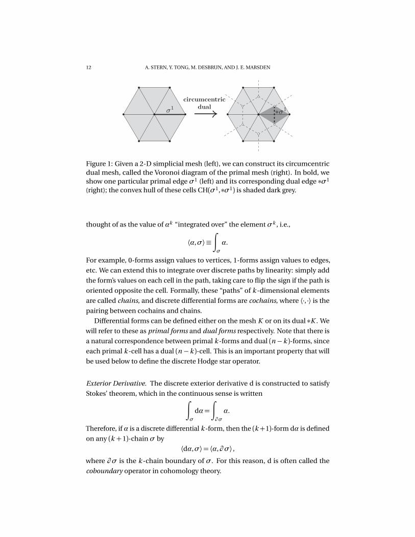
corresponding Voronoi diagram (see Figure 1). For more on the dual relationship

between Delaunay triangulations and Voronoi diagrams, a standard reference

is O’Rourke (1998). A similar construction of the circumcenter can be carried out

for higher-dimensional Euclidean simplicial complexes, as well as for simplicial

meshes in Minkowski space. Note that, in both the Euclidean and Lorentzian

cases, the circumcenter may actually lie outside the simplex if it has a very bad

aspect ratio, underscoring the importance of mesh quality for good numerical

results.

There are alternative ways to define the dual mesh—for example, placing

dual vertices at the barycenter rather than the circumcenter—but we will use

the circumcentric dual unless otherwise noted. Note that a refined definition

of the dual mesh, where dual cells at the boundary are restricted to K , will be

discussed in Section 3.3 to allow proper enforcement of boundary conditions in

computational electromagnetics.

Discrete Differential Forms. The fundamental objects of DEC are discrete dif-

ferential forms. A discrete k -form αk assigns a real number to each oriented

k -dimensional cell σk in the mesh K . (The superscripts k are not actually re-

quired by the notation, but they are often useful as reminders of what order of

form or cell we are dealing with.) This value is denoted by¬

αk ,σk¶

, and can be


Figure 1: Given a 2-D simplicial mesh (left), we can construct its circumcentricdual mesh, called the Voronoi diagram of the primal mesh (right). In bold, weshow one particular primal edge σ1 (left) and its corresponding dual edge ∗σ1

(right); the convex hull of these cells CH(σ1,∗σ1) is shaded dark grey.

thought of as the value of αk “integrated over” the elementσk , i.e.,

⟨α,σ⟩ ≡∫

σ

α.

For example, 0-forms assign values to vertices, 1-forms assign values to edges,

etc. We can extend this to integrate over discrete paths by linearity: simply add

the form’s values on each cell in the path, taking care to flip the sign if the path is

oriented opposite the cell. Formally, these “paths” of k -dimensional elements

are called chains, and discrete differential forms are cochains, where ⟨·, ·⟩ is the

pairing between cochains and chains.

Differential forms can be defined either on the mesh K or on its dual ∗K . We

will refer to these as primal forms and dual forms respectively. Note that there is

a natural correspondence between primal k -forms and dual (n −k )-forms, since

each primal k -cell has a dual (n −k )-cell. This is an important property that will

be used below to define the discrete Hodge star operator.

Exterior Derivative. The discrete exterior derivative d is constructed to satisfy

Stokes’ theorem, which in the continuous sense is written∫

σ

dα=

∫

∂ σ

α.

Therefore, if α is a discrete differential k -form, then the (k +1)-form dα is defined

on any (k +1)-chainσ by

⟨dα,σ⟩= ⟨α,∂ σ⟩ ,

where ∂ σ is the k -chain boundary of σ. For this reason, d is often called the

coboundary operator in cohomology theory.


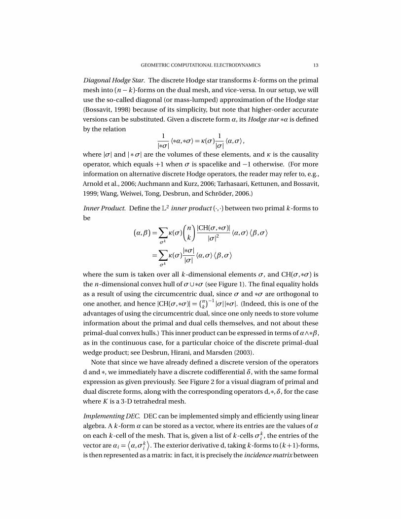
Diagonal Hodge Star. The discrete Hodge star transforms k -forms on the primal

mesh into (n −k )-forms on the dual mesh, and vice-versa. In our setup, we will

use the so-called diagonal (or mass-lumped) approximation of the Hodge star

(Bossavit, 1998) because of its simplicity, but note that higher-order accurate

versions can be substituted. Given a discrete form α, its Hodge star ∗α is defined

by the relation1

|∗σ|⟨∗α,∗σ⟩= κ(σ)

1

|σ|⟨α,σ⟩ ,

where |σ| and | ∗σ| are the volumes of these elements, and κ is the causality

operator, which equals +1 when σ is spacelike and −1 otherwise. (For more

information on alternative discrete Hodge operators, the reader may refer to, e.g.,

Arnold et al., 2006; Auchmann and Kurz, 2006; Tarhasaari, Kettunen, and Bossavit,

1999; Wang, Weiwei, Tong, Desbrun, and Schröder, 2006.)

Inner Product. Define the L2 inner product (·, ·) between two primal k -forms to

be

�

α,β�

=∑

σk

κ(σ)�

n

k

�

|CH(σ,∗σ)||σ|2

⟨α,σ⟩

β ,σ�

=∑

σk

κ(σ)|∗σ||σ|⟨α,σ⟩

β ,σ�

where the sum is taken over all k -dimensional elements σ, and CH(σ,∗σ) is

the n-dimensional convex hull ofσ∪∗σ (see Figure 1). The final equality holds

as a result of using the circumcentric dual, since σ and ∗σ are orthogonal to

one another, and hence |CH(σ,∗σ)| =�n

k

�−1 |σ| |∗σ|. (Indeed, this is one of the

advantages of using the circumcentric dual, since one only needs to store volume

information about the primal and dual cells themselves, and not about these

primal-dual convex hulls.) This inner product can be expressed in terms of α∧∗β ,

as in the continuous case, for a particular choice of the discrete primal-dual

wedge product; see Desbrun, Hirani, and Marsden (2003).

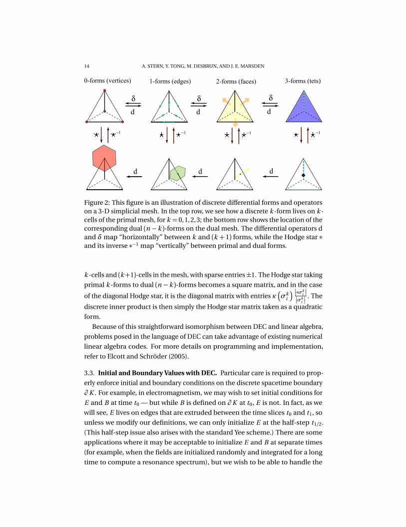
Note that since we have already defined a discrete version of the operators

d and ∗, we immediately have a discrete codifferential δ, with the same formal

expression as given previously. See Figure 2 for a visual diagram of primal and

dual discrete forms, along with the corresponding operators d,∗,δ, for the case

where K is a 3-D tetrahedral mesh.

Implementing DEC. DEC can be implemented simply and efficiently using linear

algebra. A k -form α can be stored as a vector, where its entries are the values of α

on each k -cell of the mesh. That is, given a list of k -cells σki , the entries of the

vector are αi =¬

α,σki

¶

. The exterior derivative d, taking k -forms to (k +1)-forms,

is then represented as a matrix: in fact, it is precisely the incidence matrix between


d d d

0-forms (vertices) 1-forms (edges) 2-forms (faces) 3-forms (tets)

d d d

Figure 2: This figure is an illustration of discrete differential forms and operatorson a 3-D simplicial mesh. In the top row, we see how a discrete k -form lives on k -cells of the primal mesh, for k = 0, 1, 2, 3; the bottom row shows the location of thecorresponding dual (n −k )-forms on the dual mesh. The differential operators dand δmap “horizontally” between k and (k +1) forms, while the Hodge star ∗and its inverse ∗−1 map “vertically” between primal and dual forms.

k -cells and (k+1)-cells in the mesh, with sparse entries±1. The Hodge star taking

primal k -forms to dual (n −k )-forms becomes a square matrix, and in the case

of the diagonal Hodge star, it is the diagonal matrix with entries κ�

σki

�

�

�∗σki

�

�

�

�σki

�

�

. The

discrete inner product is then simply the Hodge star matrix taken as a quadratic

form.

Because of this straightforward isomorphism between DEC and linear algebra,

problems posed in the language of DEC can take advantage of existing numerical

linear algebra codes. For more details on programming and implementation,

refer to Elcott and Schröder (2005).

3.3. Initial and Boundary Values with DEC. Particular care is required to prop-

erly enforce initial and boundary conditions on the discrete spacetime boundary

∂ K . For example, in electromagnetism, we may wish to set initial conditions for

E and B at time t0 — but while B is defined on ∂ K at t0, E is not. In fact, as we

will see, E lives on edges that are extruded between the time slices t0 and t1, so

unless we modify our definitions, we can only initialize E at the half-step t1/2.

(This half-step issue also arises with the standard Yee scheme.) There are some

applications where it may be acceptable to initialize E and B at separate times

(for example, when the fields are initialized randomly and integrated for a long

time to compute a resonance spectrum), but we wish to be able to handle the


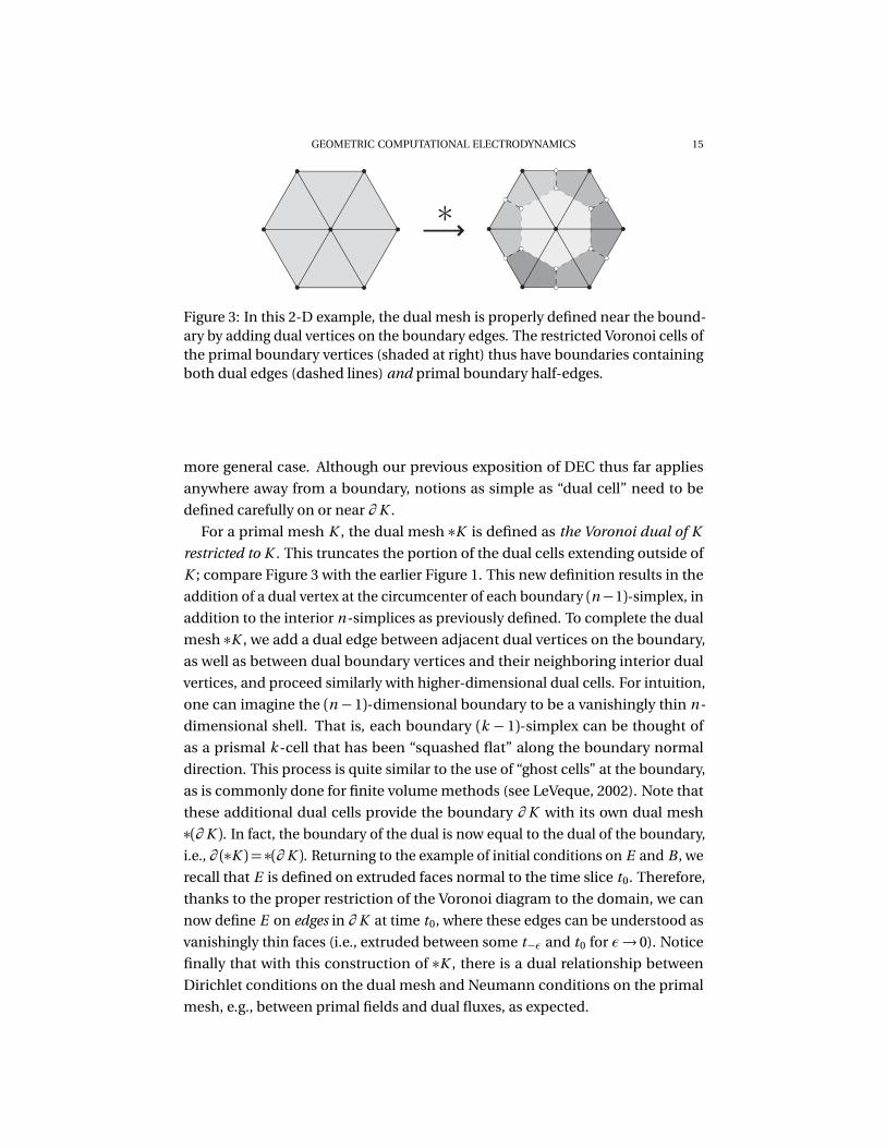
Figure 3: In this 2-D example, the dual mesh is properly defined near the bound-ary by adding dual vertices on the boundary edges. The restricted Voronoi cells ofthe primal boundary vertices (shaded at right) thus have boundaries containingboth dual edges (dashed lines) and primal boundary half-edges.

more general case. Although our previous exposition of DEC thus far applies

anywhere away from a boundary, notions as simple as “dual cell” need to be

defined carefully on or near ∂ K .

For a primal mesh K , the dual mesh ∗K is defined as the Voronoi dual of K

restricted to K . This truncates the portion of the dual cells extending outside of

K ; compare Figure 3 with the earlier Figure 1. This new definition results in the

addition of a dual vertex at the circumcenter of each boundary (n−1)-simplex, in

addition to the interior n-simplices as previously defined. To complete the dual

mesh ∗K , we add a dual edge between adjacent dual vertices on the boundary,

as well as between dual boundary vertices and their neighboring interior dual

vertices, and proceed similarly with higher-dimensional dual cells. For intuition,

one can imagine the (n −1)-dimensional boundary to be a vanishingly thin n-

dimensional shell. That is, each boundary (k − 1)-simplex can be thought of

as a prismal k -cell that has been “squashed flat” along the boundary normal

direction. This process is quite similar to the use of “ghost cells” at the boundary,

as is commonly done for finite volume methods (see LeVeque, 2002). Note that

these additional dual cells provide the boundary ∂ K with its own dual mesh

∗(∂ K ). In fact, the boundary of the dual is now equal to the dual of the boundary,

i.e., ∂ (∗K ) = ∗(∂ K ). Returning to the example of initial conditions on E and B , we

recall that E is defined on extruded faces normal to the time slice t0. Therefore,

thanks to the proper restriction of the Voronoi diagram to the domain, we can

now define E on edges in ∂ K at time t0, where these edges can be understood as

vanishingly thin faces (i.e., extruded between some t−ε and t0 for ε→ 0). Notice

finally that with this construction of ∗K , there is a dual relationship between

Dirichlet conditions on the dual mesh and Neumann conditions on the primal

mesh, e.g., between primal fields and dual fluxes, as expected.


3.4. Discrete Integration by Parts with Boundary Terms. With the dual mesh

properly defined, dual forms can now be defined on the boundary. Therefore,

the discrete duality between d and δ can be generalized to include nonvanishing

boundary terms. If α is a primal (k −1)-form and β is a primal k -form, then�

dα,β�

=�

α,δβ�

+

α∧∗β ,∂ K�

. (3.1)

In the boundary integral, α is still a primal (k − 1)-form on ∂ K , while ∗β is an

(n −k )-form taken on the boundary dual ∗(∂ K ). Formula (3.1) is readily proved

using the familiar method of discrete “summation by parts,” and thus agrees with

the integration by parts formula for smooth differential forms.

4. IMPLEMENTING MAXWELL’S EQUATIONS WITH DEC

In this section, we explain how to obtain numerical algorithms for solving

Maxwell’s equations with DEC. To do so, we will proceed in the following order.

First, we will find a sensible way to define the discrete forms F , G , and J on a

spacetime mesh. Next, we will use the DEC version of the operators d and ∗ to

obtain the discrete Maxwell’s equations. While we haven’t yet shown that these

equations are variational in the discrete sense, we will show later in Section 5

that the Lagrangian derivation of the smooth Maxwell’s equations also holds

with the DEC operators, in precisely the same way. Finally, we will discuss how

these equations can be used to define a numerical method for computational

electromagnetics.

In particular, for a rectangular grid, we will show that our setup results in the

traditional Yee scheme. For a general triangulation of space with equal time

steps, the resulting scheme will be Bossavit and Kettunen’s scheme. We will then

develop an AVI method, where each spatial element can be assigned a different

time step, and the time integration of Maxwell’s equations can be performed on

the elements asynchronously. Finally, we will comment on the equations for fully

generalized spacetime meshes, e.g., an arbitrary meshing of R3,1 by 4-simplices.

Note that the idea of discretizing Maxwell’s equations using spacetime cochains

was mentioned in, e.g., Leok (2004), as well as in a paper by Wise (2006) taking the

more abstract perspective of higher-level “p -form” versions of electromagnetism

and category theory.

4.1. Rectangular Grid. Suppose that we have a rectangular grid inR3,1, oriented

along the axes (x , y , z , t ). To simplify this exposition (although it is not necessary),

let us also suppose that the grid has uniform space and time steps∆x ,∆y ,∆z ,∆t .

Note that the DEC setup applies directly to a non-simplicial rectangular mesh,

since an n-rectangle does in fact have a circumcenter.


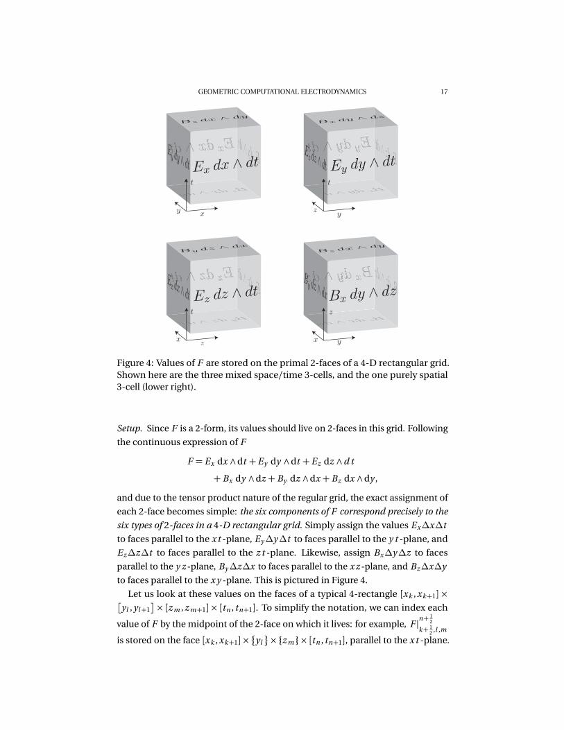
Figure 4: Values of F are stored on the primal 2-faces of a 4-D rectangular grid.Shown here are the three mixed space/time 3-cells, and the one purely spatial3-cell (lower right).

Setup. Since F is a 2-form, its values should live on 2-faces in this grid. Following

the continuous expression of F

F = Ex dx ∧dt +Ey dy ∧dt +Ez dz ∧d t

+ Bx dy ∧dz + By dz ∧dx + Bz dx ∧dy ,

and due to the tensor product nature of the regular grid, the exact assignment of

each 2-face becomes simple: the six components of F correspond precisely to the

six types of 2-faces in a 4-D rectangular grid. Simply assign the values Ex∆x∆t

to faces parallel to the x t -plane, Ey∆y∆t to faces parallel to the y t -plane, and

Ez∆z∆t to faces parallel to the z t -plane. Likewise, assign Bx∆y∆z to faces

parallel to the y z -plane, By∆z∆x to faces parallel to the x z -plane, and Bz∆x∆y

to faces parallel to the x y -plane. This is pictured in Figure 4.

Let us look at these values on the faces of a typical 4-rectangle [xk ,xk+1]×�

yl , yl+1�

× [z m , z m+1]× [tn , tn+1]. To simplify the notation, we can index each

value of F by the midpoint of the 2-face on which it lives: for example, F |n+12

k+ 12 ,l ,m

is stored on the face [xk ,xk+1]×�

yl

×{z m }× [tn , tn+1], parallel to the x t -plane.


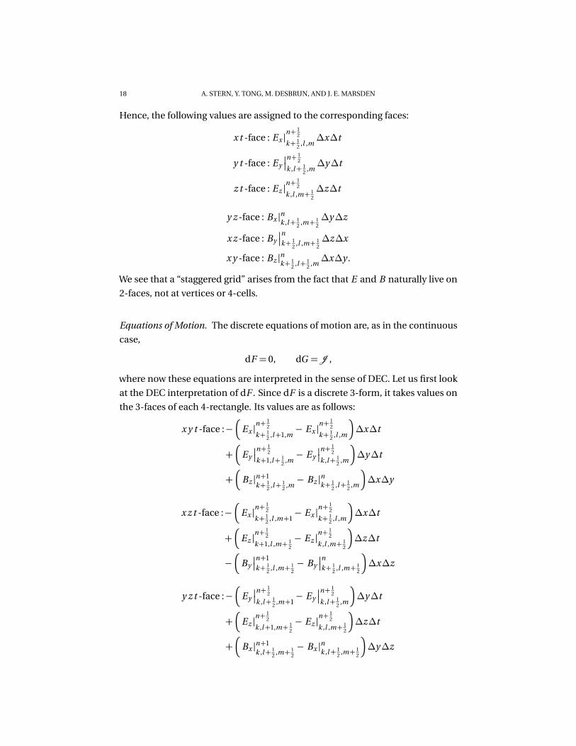
Hence, the following values are assigned to the corresponding faces:

x t -face : Ex |n+ 1

2

k+ 12 ,l ,m

∆x∆t

y t -face : Ey

�

�

n+ 12

k ,l+ 12 ,m∆y∆t

z t -face : Ez |n+ 1

2

k ,l ,m+ 12

∆z∆t

y z -face : Bx |nk ,l+ 12 ,m+ 1

2

∆y∆z

x z -face : By

�

�

n

k+ 12 ,l ,m+ 1

2∆z∆x

x y -face : Bz |nk+ 12 ,l+ 1

2 ,m∆x∆y .

We see that a “staggered grid” arises from the fact that E and B naturally live on

2-faces, not at vertices or 4-cells.

Equations of Motion. The discrete equations of motion are, as in the continuous

case,

dF = 0, dG =J ,

where now these equations are interpreted in the sense of DEC. Let us first look

at the DEC interpretation of dF . Since dF is a discrete 3-form, it takes values on

the 3-faces of each 4-rectangle. Its values are as follows:

x y t -face :−�

Ex |n+ 1

2

k+ 12 ,l+1,m

− Ex |n+ 1

2

k+ 12 ,l ,m

�

∆x∆t

+�

Ey

�

�

n+ 12

k+1,l+ 12 ,m− Ey

�

�

n+ 12

k ,l+ 12 ,m

�

∆y∆t

+�

Bz |n+1k+ 1

2 ,l+ 12 ,m− Bz |nk+ 1

2 ,l+ 12 ,m

�

∆x∆y

x z t -face :−�

Ex |n+ 1

2

k+ 12 ,l ,m+1

− Ex |n+ 1

2

k+ 12 ,l ,m

�

∆x∆t

+�

Ez |n+ 1

2

k+1,l ,m+ 12

− Ez |n+ 1

2

k ,l ,m+ 12

�

∆z∆t

−�

By

�

�

n+1

k+ 12 ,l ,m+ 1

2− By

�

�

n

k+ 12 ,l ,m+ 1

2

�

∆x∆z

y z t -face :−�

Ey

�

�

n+ 12

k ,l+ 12 ,m+1

− Ey

�

�

n+ 12

k ,l+ 12 ,m

�

∆y∆t

+�

Ez |n+ 1

2

k ,l+1,m+ 12

− Ez |n+ 1

2

k ,l ,m+ 12

�

∆z∆t

+�

Bx |n+1k ,l+ 1

2 ,m+ 12

− Bx |nk ,l+ 12 ,m+ 1

2

�

∆y∆z


x y z -face :�

Bx |nk+1,l+ 12 ,m+ 1

2

− Bx |nk ,l+ 12 ,m+ 1

2

�

∆y∆z

+�

By

�

�

n

k+ 12 ,l+1,m+ 1

2− By

�

�

n

k+ 12 ,l ,m+ 1

2

�

∆x∆z

+�

Bz |nk+ 12 ,l+ 1

2 ,m+1− Bz |nk+ 1

2 ,l+ 12 ,m

�

∆x∆y

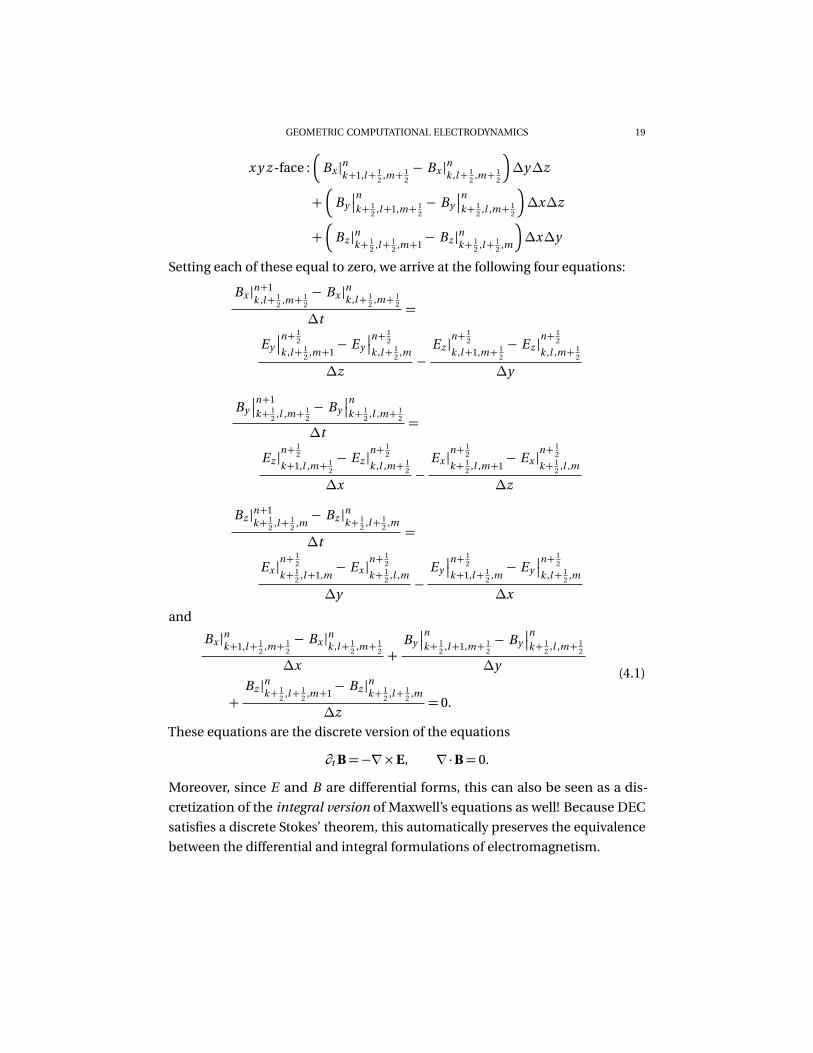
Setting each of these equal to zero, we arrive at the following four equations:

Bx |n+1k ,l+ 1

2 ,m+ 12

− Bx |nk ,l+ 12 ,m+ 1

2

∆t=

Ey

�

�

n+ 12

k ,l+ 12 ,m+1

− Ey

�

�

n+ 12

k ,l+ 12 ,m

∆z−

Ez |n+ 1

2

k ,l+1,m+ 12

− Ez |n+ 1

2

k ,l ,m+ 12

∆y

By

�

�

n+1

k+ 12 ,l ,m+ 1

2− By

�

�

n

k+ 12 ,l ,m+ 1

2

∆t=

Ez |n+ 1

2

k+1,l ,m+ 12

− Ez |n+ 1

2

k ,l ,m+ 12

∆x−

Ex |n+ 1

2

k+ 12 ,l ,m+1

− Ex |n+ 1

2

k+ 12 ,l ,m

∆z

Bz |n+1k+ 1

2 ,l+ 12 ,m− Bz |nk+ 1

2 ,l+ 12 ,m

∆t=

Ex |n+ 1

2

k+ 12 ,l+1,m

− Ex |n+ 1

2

k+ 12 ,l ,m

∆y−

Ey

�

�

n+ 12

k+1,l+ 12 ,m− Ey

�

�

n+ 12

k ,l+ 12 ,m

∆x

and

Bx |nk+1,l+ 12 ,m+ 1

2

− Bx |nk ,l+ 12 ,m+ 1

2

∆x+

By

�

�

n

k+ 12 ,l+1,m+ 1

2− By

�

�

n

k+ 12 ,l ,m+ 1

2

∆y

+Bz |nk+ 1

2 ,l+ 12 ,m+1

− Bz |nk+ 12 ,l+ 1

2 ,m

∆z= 0.

(4.1)

These equations are the discrete version of the equations

∂t B=−∇×E, ∇·B= 0.

Moreover, since E and B are differential forms, this can also be seen as a dis-

cretization of the integral version of Maxwell’s equations as well! Because DEC

satisfies a discrete Stokes’ theorem, this automatically preserves the equivalence

between the differential and integral formulations of electromagnetism.


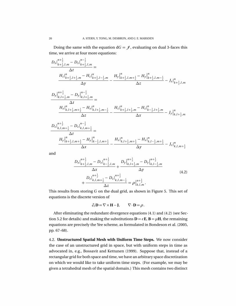
Doing the same with the equation dG = J , evaluating on dual 3-faces this

time, we arrive at four more equations:

Dx |n+ 1

2

k+ 12 ,l ,m

− Dx |n− 1

2

k+ 12 ,l ,m

∆t=

Hz |nk+ 12 ,l+ 1

2 ,m− Hz |nk+ 1

2 ,l− 12 ,m

∆y−

Hy

�

�

n

k+ 12 ,l ,m+ 1

2− Hy

�

�

n

k+ 12 ,l ,m− 1

2

∆z− Jx |nk+ 1

2 ,l ,m

Dy

�

�

n+ 12

k ,l+ 12 ,m− Dy

�

�

n− 12

k ,l+ 12 ,m

∆t=

Hx |nk ,l+ 12 ,m+ 1

2

− Hx |nk ,l+ 12 ,m− 1

2

∆z−

Hz |nk+ 12 ,l+ 1

2 ,m− Hz |nk− 1

2 ,l+ 12 ,m

∆x− Jy

�

�

n

k ,l+ 12 ,m

Dz |n+ 1

2

k ,l ,m+ 12

− Dz |n− 1

2

k ,l ,m+ 12

∆t=

Hy

�

�

n

k+ 12 ,l ,m+ 1

2− Hy

�

�

n

k− 12 ,l ,m+ 1

2

∆x−

Hx |nk ,l+ 12 ,m+ 1

2

− Hx |nk ,l− 12 ,m+ 1

2

∆y− Jz |nk ,l ,m+ 1

2

and

Dx |n+ 1

2

k+ 12 ,l ,m

− Dx |n+ 1

2

k− 12 ,l ,m

∆x+

Dy

�

�

n+ 12

k ,l+ 12 ,m− Dy

�

�

n+ 12

k ,l− 12 ,m

∆y

+Dz |

n+ 12

k ,l ,m+ 12

− Dz |n+ 1

2

k ,l ,m− 12

∆z= ρ

�

�

n+ 12

k ,l ,m.

(4.2)

This results from storing G on the dual grid, as shown in Figure 5. This set of

equations is the discrete version of

∂t D=∇×H− J, ∇·D=ρ.

After eliminating the redundant divergence equations (4.1) and (4.2) (see Sec-

tion 5.2 for details) and making the substitutions D= εE, B=µH, the remaining

equations are precisely the Yee scheme, as formulated in Bondeson et al. (2005,

pp. 67–68).

4.2. Unstructured Spatial Mesh with Uniform Time Steps. We now consider

the case of an unstructured grid in space, but with uniform steps in time as

advocated in, e.g., Bossavit and Kettunen (1999). Suppose that, instead of a

rectangular grid for both space and time, we have an arbitrary space discretization

on which we would like to take uniform time steps. (For example, we may be

given a tetrahedral mesh of the spatial domain.) This mesh contains two distinct


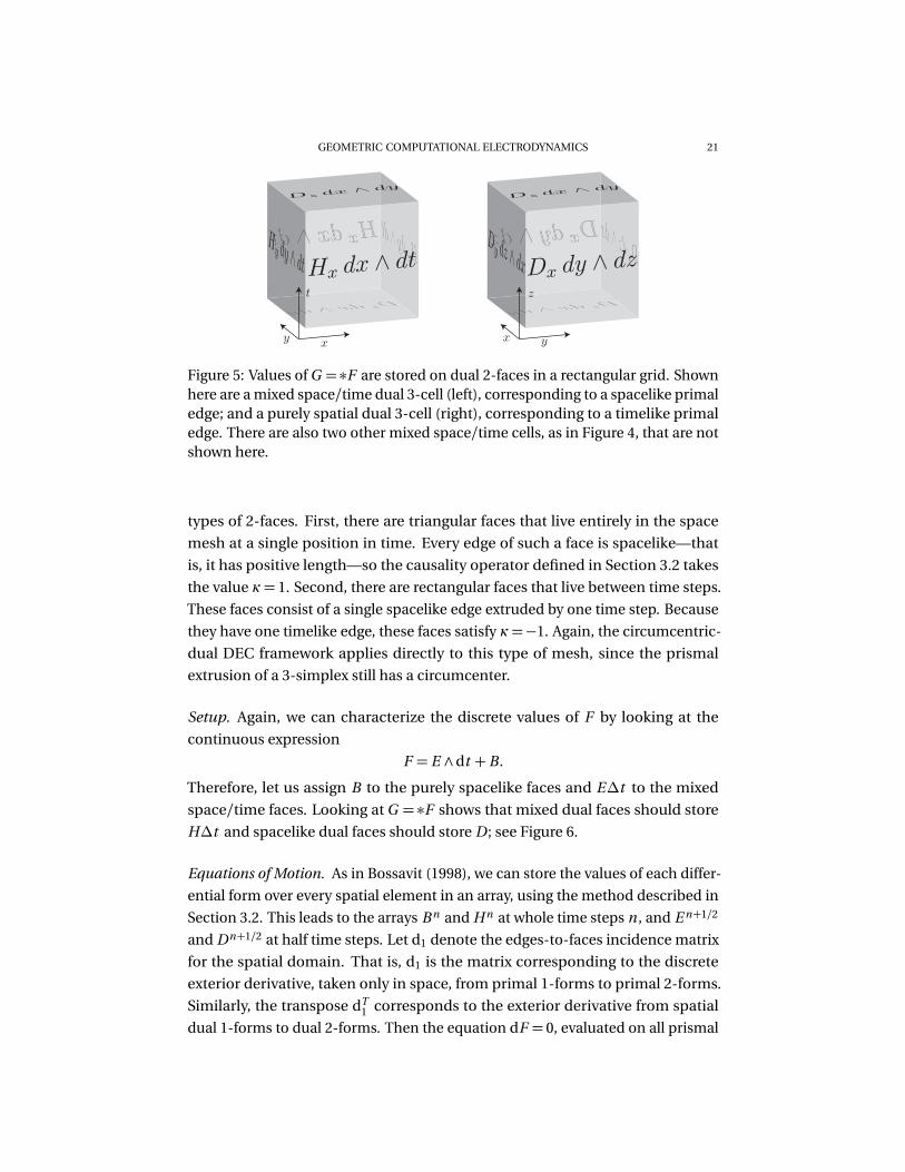
Figure 5: Values of G = ∗F are stored on dual 2-faces in a rectangular grid. Shownhere are a mixed space/time dual 3-cell (left), corresponding to a spacelike primaledge; and a purely spatial dual 3-cell (right), corresponding to a timelike primaledge. There are also two other mixed space/time cells, as in Figure 4, that are notshown here.

types of 2-faces. First, there are triangular faces that live entirely in the space

mesh at a single position in time. Every edge of such a face is spacelike—that

is, it has positive length—so the causality operator defined in Section 3.2 takes

the value κ= 1. Second, there are rectangular faces that live between time steps.

These faces consist of a single spacelike edge extruded by one time step. Because

they have one timelike edge, these faces satisfy κ=−1. Again, the circumcentric-

dual DEC framework applies directly to this type of mesh, since the prismal

extrusion of a 3-simplex still has a circumcenter.

Setup. Again, we can characterize the discrete values of F by looking at the

continuous expression

F = E ∧dt + B.

Therefore, let us assign B to the purely spacelike faces and E∆t to the mixed

space/time faces. Looking at G = ∗F shows that mixed dual faces should store

H∆t and spacelike dual faces should store D; see Figure 6.

Equations of Motion. As in Bossavit (1998), we can store the values of each differ-

ential form over every spatial element in an array, using the method described in

Section 3.2. This leads to the arrays B n and H n at whole time steps n , and E n+1/2

and Dn+1/2 at half time steps. Let d1 denote the edges-to-faces incidence matrix

for the spatial domain. That is, d1 is the matrix corresponding to the discrete

exterior derivative, taken only in space, from primal 1-forms to primal 2-forms.

Similarly, the transpose dT1 corresponds to the exterior derivative from spatial

dual 1-forms to dual 2-forms. Then the equation dF = 0, evaluated on all prismal


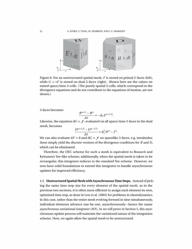
Figure 6: For an unstructured spatial mesh, F is stored on primal 2-faces (left),while G = ∗F is stored on dual 2-faces (right). Shown here are the values onmixed space/time 3-cells. (The purely spatial 3-cells, which correspond to thedivergence equations and do not contribute to the equations of motion, are notshown.)

3-faces becomesB n+1− B n

∆t=−d1E n+1/2.

Likewise, the equation dG =J , evaluated on all space/time 3-faces in the dual

mesh, becomesDn+1/2−Dn−1/2

∆t= dT

1 H n − J n .

We can also evaluate dF = 0 and dG =J on spacelike 3-faces, e.g, tetrahedra;

these simply yield the discrete versions of the divergence conditions for B and D ,

which can be eliminated.

Therefore, the DEC scheme for such a mesh is equivalent to Bossavit and

Kettunen’s Yee-like scheme; additionally, when the spatial mesh is taken to be

rectangular, this integrator reduces to the standard Yee scheme. However, we

now have solid foundations to extend this integrator to handle asynchronous

updates for improved efficiency.

4.3. Unstructured Spatial Mesh with Asynchronous Time Steps. Instead of pick-

ing the same time step size for every element of the spatial mesh, as in the

previous two sections, it is often more efficient to assign each element its own,

optimized time step, as done in Lew et al. (2003) for problems in elastodynamics.

In this case, rather than the entire mesh evolving forward in time simultaneously,

individual elements advance one-by-one, asynchronously—hence the name

asynchronous variational integrator (AVI). As we will prove in Section 5, this asyn-

chronous update process will maintain the variational nature of the integration

scheme. Here, we again allow the spatial mesh to be unstructured.


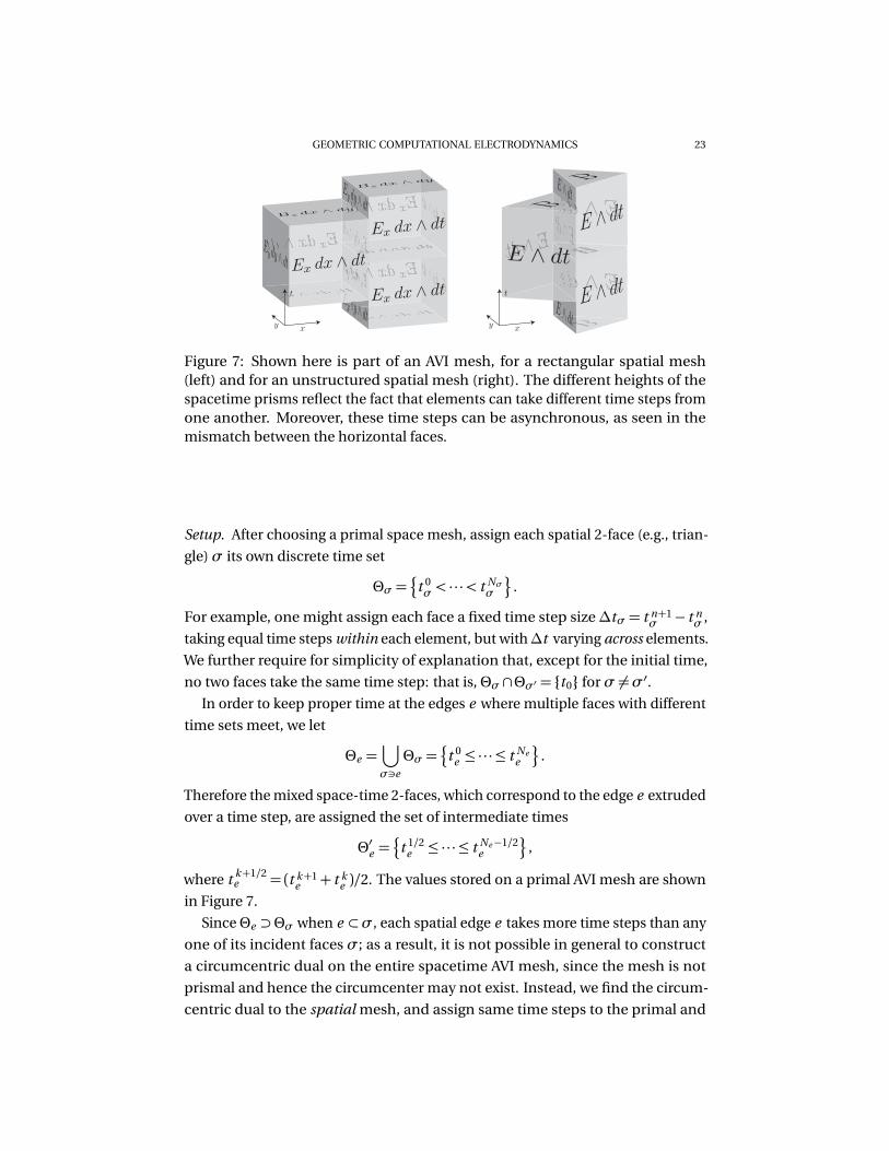
Figure 7: Shown here is part of an AVI mesh, for a rectangular spatial mesh(left) and for an unstructured spatial mesh (right). The different heights of thespacetime prisms reflect the fact that elements can take different time steps fromone another. Moreover, these time steps can be asynchronous, as seen in themismatch between the horizontal faces.

Setup. After choosing a primal space mesh, assign each spatial 2-face (e.g., trian-

gle)σ its own discrete time set

Θσ =¦

t 0σ < · · ·< t Nσ

σ

©

.

For example, one might assign each face a fixed time step size∆tσ = t n+1σ − t n

σ ,

taking equal time steps within each element, but with∆t varying across elements.

We further require for simplicity of explanation that, except for the initial time,

no two faces take the same time step: that is, Θσ ∩Θσ′ = {t0} forσ 6=σ′.In order to keep proper time at the edges e where multiple faces with different

time sets meet, we let

Θe =⋃

σ3e

Θσ =¦

t 0e ≤ · · · ≤ t Ne

e

©

.

Therefore the mixed space-time 2-faces, which correspond to the edge e extruded

over a time step, are assigned the set of intermediate times

Θ′e =¦

t 1/2e ≤ · · · ≤ t Ne−1/2

e

©

,

where t k+1/2e = (t k+1

e + t ke )/2. The values stored on a primal AVI mesh are shown

in Figure 7.

SinceΘe ⊃Θσ when e ⊂σ, each spatial edge e takes more time steps than any

one of its incident faces σ; as a result, it is not possible in general to construct

a circumcentric dual on the entire spacetime AVI mesh, since the mesh is not

prismal and hence the circumcenter may not exist. Instead, we find the circum-

centric dual to the spatial mesh, and assign same time steps to the primal and


dual elements

Θ∗σ =Θσ, Θ∗e =Θe .

This results in well-defined primal and dual cells for each 2-element in spacetime,

and hence a Hodge star for this order. (A Hodge star on forms of different order is

not needed to formulate Maxwell’s equations.)

Equations of Motion. The equation dF = 0, evaluated on a mixed space/time

3-cell, becomes

B n+1σ − B n

σ

t n+1σ − t n

σ

=−d1

∑

¦

E m+1/2e : t n

σ < t m+1/2e < t n+1

σ

©

. (4.3)

Similarly, the equation dG =J becomes

Dm+1/2e −Dm−1/2

e

t m+1/2e − t m−1/2

e

= dT1

�

H nσ1{t n

σ=t me }�

− J me , (4.4)

where 1{t nσ=t m

e } equals 1 when face σ has t nσ = t m

e for some n , and 0 otherwise.

(That is, the indicator function “picks out” the incident face that lives at the same

time step as this edge.)

Solving an initial value problem can then be summarized by the following

update loop:

(1) Pick the minimum time t n+1σ where B n+1

σ has not yet been computed.

(2) Advance B n+1σ according to Equation 4.3.

(3) Update H n+1σ = ∗−1

µ B n+1σ .

(4) Advance Dm+3/2e on neighboring edges e ⊂σ according to Equation 4.4.

(5) Update E m+3/2e = ∗−1

ε Dm+3/2e .

Iterative Time Stepping Scheme. As detailed in Lew et al. (2003) for elastody-

namics, the explicit AVI update scheme can be implemented by selecting mesh

elements from a priority queue, sorted by time, and iterating forward. However,

as written above, the scheme is not strictly iterative, since Equation 4.4 depends

on past values of E . This can be easily fixed by rewriting the AVI scheme to ad-

vance in the variables A and E instead, where the potential A effectively stores

the cumulative contribution of E to the value of B on neighboring faces. Com-

pared to the AVI for elasticity, A plays the role of the positions x, while E plays

the role of the (negative) velocities x. The algorithm is given as pseudocode in

Figure 8. Note that if all elements take uniform time steps, the AVI reduces to the

Bossavit–Kettunen scheme.

Numerical Experiments. We first present a simple numerical example demon-

strating the good energy behavior of our asynchronous integrator. The AVI was

used to integrate in time over a 2-D rectangular cavity with perfectly electrically


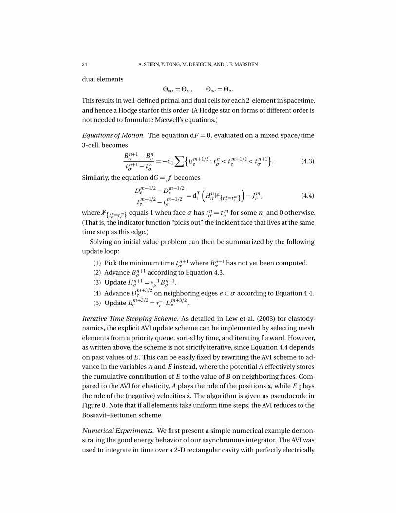
// INITIALIZE FIELDS AND PRIORITY QUEUE

for each spatial edge e doAe ← A0

e , Ee ← E 1/2e , τe ← t0 // Store initial field values and times

for each spatial faceσ doτσ← t0

Compute the next update time t 1σ

Q .push(t 1σ,σ) // Push element onto queue with its next update time

// ITERATE FORWARD IN TIME UNTIL THE PRIORITY QUEUE IS EMPTY

repeat(t ,σ)←Q .pop() // Pop next elementσ and time t from queuefor each edge e of elementσ do

Ae ← Ae −Ee (t −τe ) //Update neighboring values of A at time tif t < final-time then

Bσ← d1Ae

Hσ←∗µBσDe ←∗εEe

De ←De +d1(e ,σ)Hσ(t −τσ)Ee ←∗εDe

τσ← t //Update element’s timeCompute the next update time t next

σQ .push(t next

σ ,σ) // Scheduleσ for next updateuntil (Q .isEmpty())

Figure 8: Pseudocode for our Asynchronous Variational Integrator, implementedusing a priority queue data structure for storing and selecting the elements to beupdated.

conducting (PEC) boundaries, so that E vanishes at the boundary of the domain.

E was given random values at the initial time, so as to excite all frequency modes,

and integrated for 8 seconds. Each spatial element was given a time step equal to

1/10 of the stability-limiting time step determined by the CFL condition.

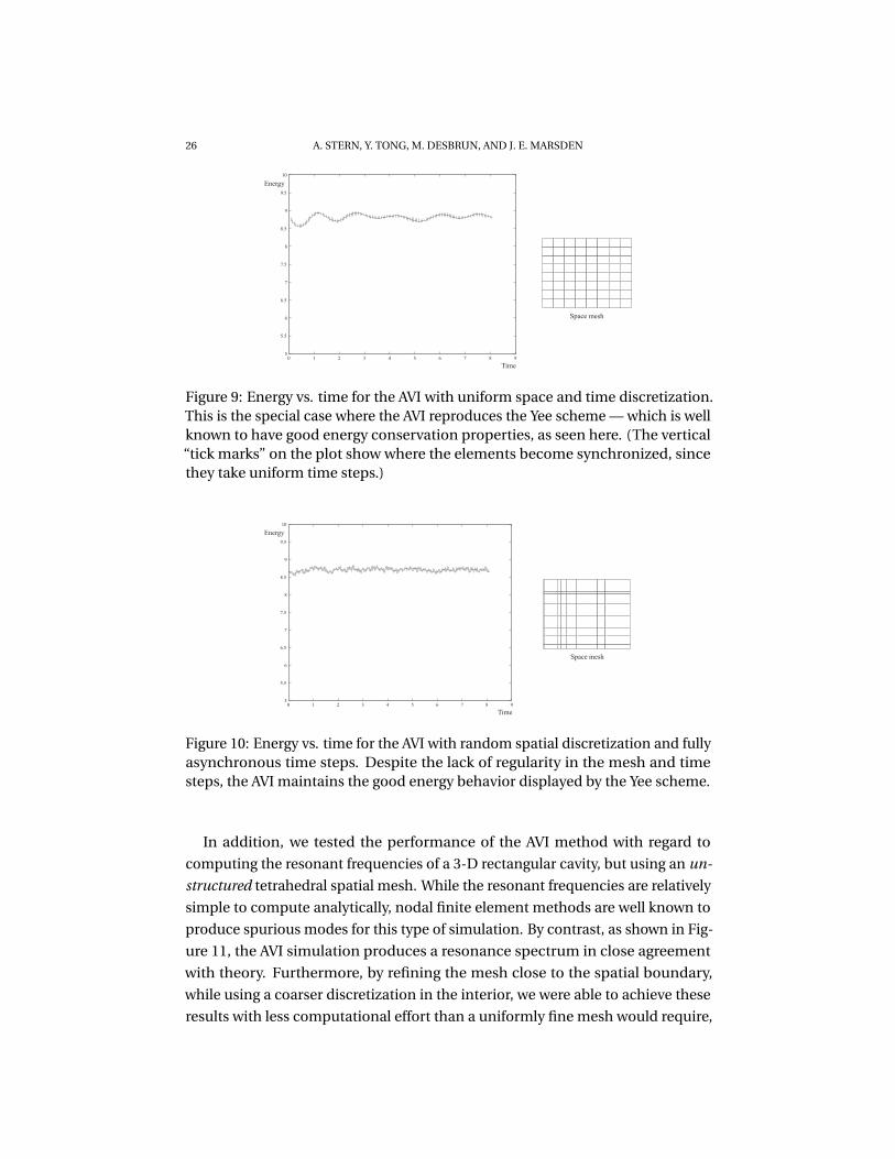
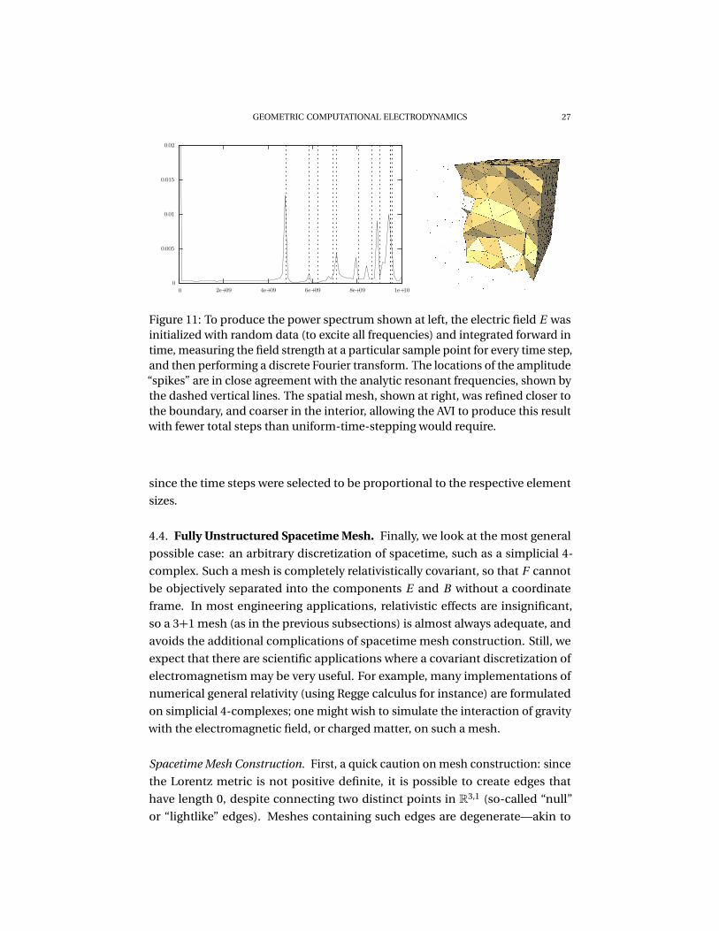
This simulation was done for two different spatial discretizations. The first

is a uniform discretization so that each element has identical time step size,

which coincides exactly with the Yee scheme. The second discretization ran-

domly partitioned the x - and y -axes, so that each element has completely unique

spatial dimensions and time step size, and so the update rule is truly asynchro-

nous. The energy plot for the uniform Yee discretization is shown in Figure 9,

while the energy for the random discretization is shown in Figure 10. Even for

a completely random, irregular mesh, our asynchronous integrator displays

near-energy preservation qualities. Such numerical behavior stems from the

variational nature of our integrator, which will be detailed in Section 5.


0 1 2 3 4 5 6 7 8 95

5.5

6

6.5

7

7.5

8

8.5

9

9.5

10

Time

Energy

Space mesh

Figure 9: Energy vs. time for the AVI with uniform space and time discretization.This is the special case where the AVI reproduces the Yee scheme — which is wellknown to have good energy conservation properties, as seen here. (The vertical“tick marks” on the plot show where the elements become synchronized, sincethey take uniform time steps.)

0 1 2 3 4 5 6 7 8 95

5.5

6

6.5

7

7.5

8

8.5

9

9.5

10

Time

Energy

Space mesh

Figure 10: Energy vs. time for the AVI with random spatial discretization and fullyasynchronous time steps. Despite the lack of regularity in the mesh and timesteps, the AVI maintains the good energy behavior displayed by the Yee scheme.

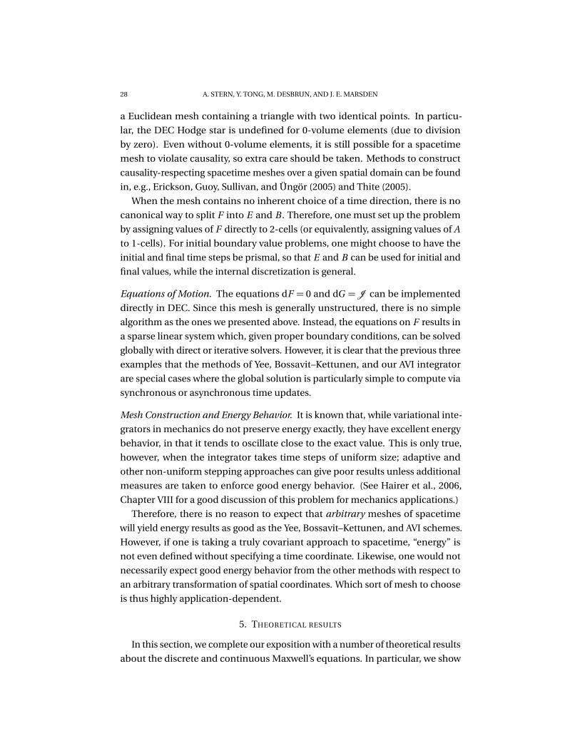
In addition, we tested the performance of the AVI method with regard to

computing the resonant frequencies of a 3-D rectangular cavity, but using an un-

structured tetrahedral spatial mesh. While the resonant frequencies are relatively

simple to compute analytically, nodal finite element methods are well known to

produce spurious modes for this type of simulation. By contrast, as shown in Fig-

ure 11, the AVI simulation produces a resonance spectrum in close agreement

with theory. Furthermore, by refining the mesh close to the spatial boundary,

while using a coarser discretization in the interior, we were able to achieve these

results with less computational effort than a uniformly fine mesh would require,


0

0.005

0.01

0.015

0.02

0 2e+09 4e+09 6e+09 8e+09 1e+10

1

Figure 11: To produce the power spectrum shown at left, the electric field E wasinitialized with random data (to excite all frequencies) and integrated forward intime, measuring the field strength at a particular sample point for every time step,and then performing a discrete Fourier transform. The locations of the amplitude“spikes” are in close agreement with the analytic resonant frequencies, shown bythe dashed vertical lines. The spatial mesh, shown at right, was refined closer tothe boundary, and coarser in the interior, allowing the AVI to produce this resultwith fewer total steps than uniform-time-stepping would require.

since the time steps were selected to be proportional to the respective element

sizes.

4.4. Fully Unstructured Spacetime Mesh. Finally, we look at the most general

possible case: an arbitrary discretization of spacetime, such as a simplicial 4-

complex. Such a mesh is completely relativistically covariant, so that F cannot

be objectively separated into the components E and B without a coordinate

frame. In most engineering applications, relativistic effects are insignificant,

so a 3+1 mesh (as in the previous subsections) is almost always adequate, and

avoids the additional complications of spacetime mesh construction. Still, we

expect that there are scientific applications where a covariant discretization of

electromagnetism may be very useful. For example, many implementations of

numerical general relativity (using Regge calculus for instance) are formulated

on simplicial 4-complexes; one might wish to simulate the interaction of gravity

with the electromagnetic field, or charged matter, on such a mesh.

Spacetime Mesh Construction. First, a quick caution on mesh construction: since

the Lorentz metric is not positive definite, it is possible to create edges that

have length 0, despite connecting two distinct points in R3,1 (so-called “null”

or “lightlike” edges). Meshes containing such edges are degenerate—akin to


a Euclidean mesh containing a triangle with two identical points. In particu-

lar, the DEC Hodge star is undefined for 0-volume elements (due to division

by zero). Even without 0-volume elements, it is still possible for a spacetime

mesh to violate causality, so extra care should be taken. Methods to construct

causality-respecting spacetime meshes over a given spatial domain can be found

in, e.g., Erickson, Guoy, Sullivan, and Üngör (2005) and Thite (2005).

When the mesh contains no inherent choice of a time direction, there is no

canonical way to split F into E and B . Therefore, one must set up the problem

by assigning values of F directly to 2-cells (or equivalently, assigning values of A

to 1-cells). For initial boundary value problems, one might choose to have the

initial and final time steps be prismal, so that E and B can be used for initial and

final values, while the internal discretization is general.

Equations of Motion. The equations dF = 0 and dG =J can be implemented

directly in DEC. Since this mesh is generally unstructured, there is no simple

algorithm as the ones we presented above. Instead, the equations on F results in

a sparse linear system which, given proper boundary conditions, can be solved

globally with direct or iterative solvers. However, it is clear that the previous three

examples that the methods of Yee, Bossavit–Kettunen, and our AVI integrator

are special cases where the global solution is particularly simple to compute via

synchronous or asynchronous time updates.

Mesh Construction and Energy Behavior. It is known that, while variational inte-

grators in mechanics do not preserve energy exactly, they have excellent energy

behavior, in that it tends to oscillate close to the exact value. This is only true,

however, when the integrator takes time steps of uniform size; adaptive and

other non-uniform stepping approaches can give poor results unless additional

measures are taken to enforce good energy behavior. (See Hairer et al., 2006,

Chapter VIII for a good discussion of this problem for mechanics applications.)

Therefore, there is no reason to expect that arbitrary meshes of spacetime

will yield energy results as good as the Yee, Bossavit–Kettunen, and AVI schemes.

However, if one is taking a truly covariant approach to spacetime, “energy” is

not even defined without specifying a time coordinate. Likewise, one would not

necessarily expect good energy behavior from the other methods with respect to

an arbitrary transformation of spatial coordinates. Which sort of mesh to choose

is thus highly application-dependent.

5. THEORETICAL RESULTS

In this section, we complete our exposition with a number of theoretical results

about the discrete and continuous Maxwell’s equations. In particular, we show


that the DEC formulation of electromagnetism derives from a discrete Lagrangian

variational principle, and that this formulation is consequently multisymplectic.

Furthermore, we explore the gauge symmetry of Maxwell’s equations, and detail

how a particular choice of gauge eliminates the equation for∇·D−ρ from the

Euler–Lagrange equations, while preserving it automatically as a momentum

map.

Theorem 5.1. The discrete Maxwell’s equations are variational.

Proof. The idea of this proof is to emulate the derivation of the continuous

Maxwell’s equations from Section 2. Interpreting this in the sense of DEC, we will

obtain the discrete Maxwell’s equations.

Given a discrete 1-form A and dual source 3-form J , define the discrete

Lagrangian 4-form

Ld =−1

2dA ∧∗dA +A ∧J ,

with the corresponding discrete action principle

Sd [A] = ⟨Ld , K ⟩ .

Then, taking a discrete 1-form variation α vanishing on the boundary, the corre-

sponding variation of the action is

dSd [A] ·α=

−dα∧∗dA +α∧J , K�

=

α∧�

−d∗dA +J�

, K�

.

(Here we use the bold d to indicate that we are differentiating over the smooth

space of discrete forms A, as opposed to differentiating over discrete spacetime, for

which we use d.) Setting this equal to 0 for all variations α, the resulting discrete

Euler–Lagrange equations are therefore d∗dA =J . Defining the discrete 2-forms

F = dA and G = ∗F , this implies dF = 0 and dG = J , the discrete Maxwell’s

equations. �

5.1. Multisymplecticity. The concept of multisymplecticity for Lagrangian field

theories was developed in Marsden et al. (1998), where it was shown to arise from

the boundary terms for general variations of the action, i.e., those not restricted

to vanish at the boundary. As originally presented, the Cartan form θL is an

(n + 1)-form, where the n-dimensional boundary integral is then obtained by

contracting θL with a variation. The multisymplectic (n + 2)-formωL is then

given by ωL = −dθL . Contracting ωL with two arbitrary variations gives an

n-form that vanishes when integrated over the boundary, a result called the

multisymplectic form formula, which results from the identity d2 = 0. In the

special case of mechanics, where n = 0, the boundary consists of the initial and

final time points; hence, this implies the usual result that the symplectic 2-form

ωL is preserved by the time flow.


Alternatively, as communicated to us by Patrick (2004), one can view the Cartan

form θL as an n-form-valued 1-form, and the multisymplectic formωL as an

n-form-valued 2-form. Therefore, one simply evaluates these forms on tangent

variations to obtain a boundary integral, rather than taking contractions. These

two formulations are equivalent on smooth spaces. However, we will adopt

Patrick’s latter definition, since it is more easily adapted to problems on discrete

meshes: θL and ωL remain smooth 1- and 2-forms, respectively, but their n-

form values are now taken to be discrete. See Figure 12 for an illustration of the

discrete multisymplectic form formula.

Theorem 5.2. The discrete Maxwell’s equations are multisymplectic.

Proof. Let K ⊂K be an arbitrary subcomplex, and consider the discrete action

functional Sd restricted to K . Suppose now that we take a discrete variation α,

without requiring it to vanish on the boundary ∂ K . Then variations of the action

contain an additional boundary term

dSd [A] ·α=

α∧�

−d∗dA +J�

, K�

+ ⟨α∧∗d A,∂ K ⟩ .

Restricting to the space of potentials A that satisfy the discrete Euler–Lagrange

equations, the first term vanishes, leaving only

dSd (A) ·α= ⟨α∧∗dA,∂ K ⟩ (5.1)

Then we can define the Cartan form θLd by

θLd ·α=α∧∗dA.

Since θLd takes a tangent vector α and produces a discrete 3-form on the bound-

ary of the subcomplex, it is a smooth 1-form taking discrete 3-form values. Now,

since the space of discrete forms is itself actually continuous, we can take the

exterior derivative in the smooth sense on both sides of Equation 5.1. Evaluating

along another first variation β (again restricted to the space of Euler–Lagrange

solutions), we then get

d2Sd [A] ·α ·β =

dθ ·α ·β ,∂ K�

.

Finally, defining the multisymplectic formωLd =−dθLd , and using the fact that

d2Sd = 0, we get the relation

ωLd ·α ·β ,∂ K�

= 0 (5.2)

for all variations α,β ; Equation 5.2 is a discrete version of the multisymplec-

tic form formula. Since this holds for any subcomplex K , it follows that these

schemes are multisymplectic. �


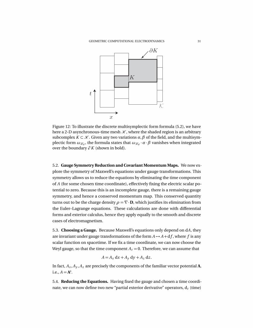
Figure 12: To illustrate the discrete multisymplectic form formula (5.2), we havehere a 2-D asynchronous-time meshK , where the shaded region is an arbitrarysubcomplex K ⊂K . Given any two variations α,β of the field, and the multisym-plectic form ωLd , the formula states that ωLd ·α ·β vanishes when integratedover the boundary ∂ K (shown in bold).

5.2. Gauge Symmetry Reduction and Covariant Momentum Maps. We now ex-

plore the symmetry of Maxwell’s equations under gauge transformations. This

symmetry allows us to reduce the equations by eliminating the time component

of A (for some chosen time coordinate), effectively fixing the electric scalar po-

tential to zero. Because this is an incomplete gauge, there is a remaining gauge

symmetry, and hence a conserved momentum map. This conserved quantity

turns out to be the charge density ρ =∇·D, which justifies its elimination from

the Euler–Lagrange equations. These calculations are done with differential

forms and exterior calculus, hence they apply equally to the smooth and discrete

cases of electromagnetism.

5.3. Choosing a Gauge. Because Maxwell’s equations only depend on dA, they

are invariant under gauge transformations of the form A 7→ A+d f , where f is any

scalar function on spacetime. If we fix a time coordinate, we can now choose the

Weyl gauge, so that the time component A t = 0. Therefore, we can assume that

A = Ax dx +Ay dy +Az dz .

In fact, Ax , Ay , Az are precisely the components of the familiar vector potential A,

i.e., A =A[.

5.4. Reducing the Equations. Having fixed the gauge and chosen a time coordi-

nate, we can now define two new “partial exterior derivative” operators, dt (time)


and ds (space), where d= dt +ds . Since A contains no dt terms, ds A is a 2-form

containing only the space terms of dA, while dt A contains the terms involving

both space and time. That is,

dt A = E ∧dt , ds A = B.

Restricted to this subspace of potentials, the Lagrangian density then becomes

L =−1

2(dt A +ds A)∧∗ (dt A +ds A)+A ∧J

=−1

2(dt A ∧∗dt A +ds A ∧∗ds A)+A ∧ J ∧dt

Next, varying the action along a restricted variation α that vanishes on ∂ X ,

dS[A] ·α=∫

X

(dtα∧D −dsα∧H ∧dt +α∧ J ∧dt ) (5.3)

=

∫

X

α∧ (dt D −ds H ∧dt + J ∧dt ) .

Setting this equal to zero by Hamilton’s principle, one immediately gets Ampère’s

law as the sole Euler–Lagrange equation. The divergence constraint ds D = ρ,

corresponding to Gauss’ law, has been eliminated via the restriction to the Weyl

gauge.

Noether’s Theorem Implies Automatic Preservation of Gauss’ Law. Let us restrict

A to be an Euler–Lagrange solution in the Weyl gauge, but remove the previous

requirement that variationsα be fixed at the initial time t0 and final time t f . Then,

varying the action along this new α, the Euler–Lagrange term disappears, but we

now pick up an additional boundary term due to integration by parts

dS[A] ·α=∫

Σ

α∧D

�

�

�

�

�

t f

t0

,

where Σ denotes a Cauchy surface of X , corresponding to the spatial domain. If

we vary along a gauge transformation α= ds f , then this becomes

dS[A] ·ds f =

∫

Σ

ds f ∧D

�

�

�

�

�

t f

t0

=−∫

Σ

f ∧ds D

�

�

�

�

�

t f

t0

Alternatively, plugging α= ds f into Equation 5.3, we get

dS[A] ·ds f =

∫

X

ds f ∧ J ∧dt =−∫

X

f ∧ds J ∧dt =−∫

X

f ∧dtρ =−∫

Σ

f ∧ρ

�

�

�

�

�

t f

t0

.


Since these two expressions are equal, and f is an arbitrary function, it follows

that�

ds D −ρ�

�

�

t f

t0= 0.

This indicates that ds D −ρ is a conserved quantity, a momentum map, so if

Gauss’ law holds at the initial time, then it holds for all subsequent times as well.

5.5. Boundary Conditions and Variational Structure. It should be noted that

the variational structure and symmetry of Maxwell’s equations may be affected by

the boundary conditions that one chooses to impose. There are many boundary

conditions that one can specify independent of the initial values, such as the

PEC condition used in the numerical example in Section 4.3. However, one can

imagine more complicated boundary conditions where which the boundary

interacts nontrivially with the interior of the domain — such as dissipative or

forced boundary conditions, where energy/momentum is removed from or added

to the system. In these cases, one will obviously not conclude that the charge

density∇·D is conserved, but more generally that the change in charge is related

to the flux through the spatial boundary. This is because, in the momentum

map derivation above, the values of f on the initial time slice causally affects its

values on the spatial boundary at intermediate times, not just on the final time

slice. Thus, the spatial part of ∂ X cannot be neglected for arbitrary boundary

conditions.

6. CONCLUSION

The continued success of the Yee scheme for many applications of computa-

tional electromagnetism, for over four decades, illustrates the value of structure-

preserving numerical integrators for Maxwell’s equations. Recent advances by,

among others, Bossavit and Kettunen, and Gross and Kotiuga, have demon-

strated the important role of compatible spatial discretization using differential

forms, allowing for Yee-like schemes that apply on generalized spatial meshes.

In this paper, we have extended this approach by considering discrete forms on

spacetime, encapsulating both space and time discretization, and have derived a

general family of geometric numerical integrators for Maxwell’s equations. Fur-

thermore, since we have derived these integrators from a discrete variational

principle, the resulting methods are provably multisymplectic and momentum-

map-preserving, and they experimentally show correct global energy behavior.

Besides proving the variational nature of well-known techniques such as the Yee

and Bossavit–Kettunen schemes, we have also introduced a new asynchronous

integrator, so that time step sizes can be taken non-uniformly over the spatial


domain for increased efficiency, while still maintaining the desirable variational

and energy behavior of the other methods.

Future Work. One promising avenue for future work involves increasing the

order of accuracy of these methods by deriving higher-order discrete Hodge star

operators. While this would involve redefining the Hodge star matrix to be non-

diagonal, the discrete Maxwell’s equations would remain formally the same, and

hence there would be no change in the variational or multisymplectic properties

proven here. We are currently exploring the development of a spectrally accurate

spatial Hodge star, which might make these geometric schemes competitive for

applications where non-variational spectral codes are currently favored.

Additionally, the recent work of Kale and Lew (2007) has shown that AVIs can

be implemented as parallel algorithms for solid mechanics simulations. This

uses the fact that, due to the asynchronous update procedure, an element does

not need information from every one of its neighbors at every time step, which

lessens the need for communication among parallel nodes. The resulting parallel

AVIs, or PAVIs, can therefore take advantage of parallel computing architecture

for improved efficiency. It is reasonable to expect that the same might be done in

the case of our electromagnetic AVI.

While we have experimentally observed the fact that variational integrators

exhibit near-energy conservation, little is known about this behavior from a theo-

retical standpoint. In the case of ODEs in mechanics, backwards error analysis

has shown that these methods exactly integrate a nearby smooth Hamiltonian

system, although not much known about how this relates to the discrete varia-

tional principle on the Lagrangian side. Some initial work has been done in Oliver,

West, and Wulff (2004) to understand, also by a backward error analysis approach,

why discrete multisymplectic methods also display good energy behavior.

Finally, variational methods using discrete spacetime forms may be developed

for field theories other than electromagnetism. Promising candidates include nu-

merical general relativity and fluid dynamics, although the latter is complicated

by the difficulty in finding a proper discretization of the infinite-dimensional

diffeomorphism group. If discrete Lagrangian densities are developed for these

theories, it should be straightforward to combine them with the electromagnetic

Lagrangian, resulting in numerical methods to simulate, e.g., gravity coupled

with an electromagnetic field, or the dynamics of a charged or magnetic fluid.

ACKNOWLEDGMENTS

We would like to thank several people for their inspiration and suggestions.

First of all, Alain Bossavit for suggesting many years ago that we take the present


DEC approach to computational electromagnetism, and for his excellent lectures

at Caltech on the subject. Second, Michael Ortiz and Eva Kanso for their ongoing

interactions on related topics and suggestions. We also thank Doug Arnold,

Uri Ascher, Robert Kotiuga, Melvin Leok, Adrian Lew, and Matt West for their

feedback and encouragement. In addition, the 3-D AVI simulations shown in

Figure 11 were programmed and implemented by Patrick Xia, as part of a Summer

Undergraduate Research Fellowship at Caltech.

REFERENCES

Arnold, D. N., R. S. Falk, and R. Winther (2006), Finite element exterior calculus,

homological techniques, and applications. Acta Numer., 15, 1–155.

Auchmann, B., and S. Kurz (2006), A geometrically defined discrete Hodge opera-

tor on simplicial cells. IEEE Trans. Magn., 42 (4), 643–646.

Bondeson, A., T. Rylander, and P. Ingelström (2005), Computational electromag-

netics, volume 51 of Texts in Applied Mathematics. Springer, New York.

Bossavit, A. (1998), Computational electromagnetism. Electromagnetism, Aca-

demic Press Inc., San Diego, CA. Variational formulations, complementarity,

edge elements.

Bossavit, A., and L. Kettunen (1999), Yee-like schemes on a tetrahedral mesh, with

diagonal lumping. Int. J. Numer. Modell., 12 (1–2), 129–142.

Bossavit, A., and L. Kettunen (2000), Yee-like schemes on staggered cellular grids:

A synthesis between FIT and FEM approaches. IEEE Trans. Magn., 36 (4), 861–

867.

Clemens, M., and T. Weiland (2002), Magnetic field simulation using conformal

FIT formulations. IEEE Trans. Magn., 38 (2), 389–392.

Desbrun, M., A. N. Hirani, and J. E. Marsden (2003), Discrete exterior calculus

for variational problems in computer vision and graphics. In Proceedings of

the 42nd IEEE Conference on Decision and Control (CDC), volume 5, pages

4902–4907. IEEE Press, Washington, DC.

Desbrun, M., E. Kanso, and Y. Tong (2008), Discrete differential forms for compu-

tational modeling. In Discrete differential geometry, volume 38 of Oberwolfach

Semin., pages 287–324. Birkhäuser, Basel.

Elcott, S., and P. Schröder (2005), Building your own DEC at home. In

SIGGRAPH ’05: ACM SIGGRAPH 2005 Courses. ACM Press, New York.

doi:10.1145/1198555.1198667.

Erickson, J., D. Guoy, J. Sullivan, and A. Üngör (2005), Building spacetime meshes

over arbitrary spatial domains. Engineering with Computers, 20 (4), 342–353.

doi:10.1007/s00366-005-0303-0.

http://dx.doi.org/10.1145/1198555.1198667

http://dx.doi.org/10.1007/s00366-005-0303-0


Gross, P. W., and P. R. Kotiuga (2004), Electromagnetic theory and computation: a

topological approach, volume 48 of Mathematical Sciences Research Institute

Publications. Cambridge University Press, Cambridge.

Haber, E., and U. M. Ascher (2001), Fast finite volume simulation of 3D electro-

magnetic problems with highly discontinuous coefficients. SIAM J. Sci. Com-

put., 22 (6), 1943–1961.

Hairer, E., C. Lubich, and G. Wanner (2006), Geometric numerical integration,

volume 31 of Springer Series in Computational Mathematics. Springer-Verlag,

Berlin, second edition. Structure-preserving algorithms for ordinary differential

equations.

Harrison, J. (2005), Ravello lecture notes on geometric calculus—Part I. Preprint.

arXiv:math-ph/0501001.

Hirani, A. N. (2003), Discrete exterior calculus. Ph.D. thesis, California Insti-

tute of Technology. Available from: http://resolver.caltech.edu/

CaltechETD:etd-05202003-095403.

Kale, K. G., and A. J. Lew (2007), Parallel asynchronous variational integrators.

Internat. J. Numer. Methods Engrg., 70 (3), 291–321.

Leok, M. (2004), Foundations of computational geometric mechanics. Ph.D. the-

sis, California Institute of Technology. Available from: http://resolver.

caltech.edu/CaltechETD:etd-03022004-000251.

LeVeque, R. J. (2002), Finite volume methods for hyperbolic problems. Cambridge

Texts in Applied Mathematics, Cambridge University Press, Cambridge.

Lew, A., J. E. Marsden, M. Ortiz, and M. West (2003), Asynchronous variational

integrators. Arch. Ration. Mech. Anal., 167 (2), 85–146.

Lew, A., J. E. Marsden, M. Ortiz, and M. West (2004), Variational time integrators.

Internat. J. Numer. Methods Engrg., 60 (1), 153–212.

Marsden, J. E., G. W. Patrick, and S. Shkoller (1998), Multisymplectic geometry,

variational integrators, and nonlinear PDEs. Comm. Math. Phys., 199 (2), 351–

395.

Marsden, J. E., S. Pekarsky, S. Shkoller, and M. West (2001), Variational methods,

multisymplectic geometry and continuum mechanics. J. Geom. Phys., 38 (3-4),

253–284.

Marsden, J. E., and M. West (2001), Discrete mechanics and variational integrators.

Acta Numer., 10, 357–514.

Nédélec, J.-C. (1980), Mixed finite elements inR3. Numer. Math., 35 (3), 315–341.

Oliver, M., M. West, and C. Wulff (2004), Approximate momentum conservation

for spatial semidiscretizations of semilinear wave equations. Numer. Math., 97

(3), 493–535.

http://arxiv.org/abs/math-ph/0501001

http://resolver.caltech.edu/CaltechETD:etd-05202003-095403





O’Rourke, J. (1998), Computational geometry in C. Cambridge University Press,

Cambridge, second edition.

Patrick, G. W. (2004), Geometric classical field theory. Personal communication.

Tarhasaari, T., L. Kettunen, and A. Bossavit (1999), Some realizations of a discrete

Hodge operator: a reinterpretation of finite element techniques. IEEE Trans.

Magn., 35 (3), 1494–1497.

Thite, S. (2005), Spacetime meshing for discontinuous Galerkin methods. Ph.D.

thesis, University of Illinois at Urbana-Champaign.

Wang, K., Weiwei, Y. Tong, M. Desbrun, and P. Schröder (2006), Edge subdi-

vision schemes and the construction of smooth vector fields. In SIGGRAPH

’06: ACM SIGGRAPH 2006 Papers, pages 1041–1048. ACM Press, New York.

doi:10.1145/1179352.1141991.

Whitney, H. (1957), Geometric integration theory. Princeton University Press,

Princeton, NJ.

Wise, D. K. (2006), p -form electromagnetism on discrete spacetimes. Classical

Quantum Gravity, 23 (17), 5129–5176.

Yee, K. S. (1966), Numerical solution of inital boundary value problems involving

Maxwell’s equations in isotropic media. IEEE Trans. Ant. Prop., 14 (3), 302–307.

Yoshimura, H., and J. E. Marsden (2006), Dirac structures in Lagrangian mechan-

ics. II. Variational structures. J. Geom. Phys., 57 (1), 209–250.

DEPARTMENT OF APPLIED AND COMPUTATIONAL MATHEMATICS, CALIFORNIA INSTITUTE OF TECHNOL-

OGY, PASADENA CA 91125

Current address: Department of Mathematics, University of California, San Diego, La Jolla CA

92093-0112

E-mail address: [email protected]

DEPARTMENT OF COMPUTER SCIENCE, CALIFORNIA INSTITUTE OF TECHNOLOGY, PASADENA CA 91125

Current address: Department of Computer Science and Engineering, Michigan State University,

East Lansing MI 48824


DEPARTMENT OF COMPUTER SCIENCE, CALIFORNIA INSTITUTE OF TECHNOLOGY, PASADENA CA 91125


CONTROL AND DYNAMICAL SYSTEMS, CALIFORNIA INSTITUTE OF TECHNOLOGY, PASADENA CA 91125


http://dx.doi.org/10.1145/1179352.1141991

geometric computational electrodynamics with … computational electrodynamics with variational...

Documents