variable speed drive loadshape project · water source heat pump circulation pumps (whp) these five...
TRANSCRIPT

Variable Speed Drive Loadshape Project
August 2014
Northeast Energy Efficiency Partnerships 91 Hartwell Avenue Lexington, MA 02421 P: 781.860.9177 www.neep.org
2
About NEEP & the Regional EM&V Forum
NEEP was founded in 1996 as a non-profit whose mission is to serve the Northeast and Mid-Atlantic to accelerate energy
efficiency in the building sector through public policy, program strategies and education. Our vision is that the region will fully embrace energy efficiency as a cornerstone of sustainable energy policy to help achieve a cleaner environment and
a more reliable and affordable energy system.
The Regional Evaluation, Measurement and Verification Forum (EM&V Forum or Forum) is a project facilitated by Northeast Energy Efficiency Partnerships, Inc. (NEEP). The Forum’s purpose is to provide a framework for the development and use of common and/or consistent protocols to measure, verify, track, and report energy efficiency and
other demand resource savings, costs, and emission impacts to support the role and credibility of these resources in current and emerging energy and environmental policies and markets in the Northeast, New York, and the Mid-Atlantic
region.
About Cadmus
The Cadmus Group, Inc. (Cadmus) is a nationally recognized energy and environmental consulting firm committed to
delivering services and solutions that create social and economic value and improve people’s lives. Our multidisciplinary staff of professionals provides technical expertise across the full spectrum of energy, environmental, public health, and sustainability consulting. The Energy Services Division at Cadmus works with utilities, regulatory commissions, and other
organizations to provide comprehensive services that encompass all aspects of energy efficiency and demand response program planning, design, and evaluation; renewables and distributed generation; and carbon and greenhouse gas
emissions.

Variable Speed Drive
Loadshape Project
FINAL REPORT August 15, 2014
Northeast Energy Efficiency Partnerships
Regional Evaluation, Measurement and Verification Forum
91 Hartwell Avenue
Lexington, MA 02421

This page left blank.
Prepared by:
Arlis Reynolds
Jennifer Huckett, Ph.D.
Andrew Wood
Dave Korn
Jay Robbins, DMI
Cadmus: Energy Services Division

This page left blank.

Table of Contents 0 Executive Summary .......................................................................................................................i
0.1 Objective ..............................................................................................................................i
0.2 Methods...............................................................................................................................i
0.3 Results ............................................................................................................................. viii
0.4 Recommendations ............................................................................................................xvii
1 Introduction .................................................................................................................................1
1.1 NEEP EM&V Forum ..............................................................................................................1
1.2 Project Objectives and Scope ................................................................................................2
1.3 Definitions ...........................................................................................................................2
1.4 Acknowledgements ..............................................................................................................4
2 Methods ......................................................................................................................................5
2.1 Sample Design .....................................................................................................................5
2.2 Sample Draw and Project Recruitment ................................................................................ 20
2.3 Data Collection .................................................................................................................. 22
2.4 Data Analysis ..................................................................................................................... 28
2.5 Sample Analysis ................................................................................................................. 44
3 Results ....................................................................................................................................... 51
3.1 Final Study Sample ............................................................................................................. 51
3.2 Observations on VSD Operation .......................................................................................... 51
3.3 Pre-Retrofit Operation ....................................................................................................... 55
3.4 Savings Results .................................................................................................................. 57
4 Recommendations...................................................................................................................... 71

Table of Figures
Figure 1. Examples of Hourly Models for Temperature-Dependent Units ............................................... v
Figure 2. Calculation for the Unit-Level Savings Loadshape.................................................................. vii
Figure 3. Distribution of Motor Sizes (motor hp) by Equipment Type .................................................... ix
Figure 4. Distribution of Building Types in Final Sample ......................................................................... x
Figure 5. Examples of Observed Variation in VSD Operation ................................................................. xi
Figure 6. Key Tasks for Loadshape Analysis ...........................................................................................5
Figure 7. Diagram of Multi-Stage, Multi-Phase Sample Strategy........................................................... 12
Figure 8. Review Recruitment Process for Sampled Projects ................................................................ 21
Figure 9. Example of Installed Power-Metering Kit .............................................................................. 27
Figure 10. Process for Estimating Unit-Level Savings Loadshapes and Metrics ...................................... 29
Figure 11. Example of Preliminary Data Review .................................................................................. 31
Figure 12. Example of Unit Operating Schedule .................................................................................. 33
Figure 13. Process to Determine VSD Power Model ............................................................................ 35
Figure 14. Sample Unit with Constant Power for All Hours .................................................................. 35
Figure 15. Examples of Hourly Models for Temperature-Dependent Units ........................................... 37
Figure 16. Process for Estimating Baseline Demand Loadshapes .......................................................... 39
Figure 17. eQUEST Fan System Power-Flow Performance Curves ......................................................... 41
Figure 18. Fan Systems Normalized to VFD (shown as y=x) .................................................................. 42
Figure 19. Average Pre-Installation Power from Massachusetts Pre/Post Study Metering ..................... 43
Figure 20. Calculation for the Unit-Level Savings Loadshape ................................................................ 43
Figure 21. Process for Defining the Sample Analysis Method ............................................................... 45
Figure 22. Calculation Steps for Population Analysis ............................................................................ 47
Figure 23. Examples of Observed Variation in VSD Operation .............................................................. 52
Figure 24. Population Results for Supply Fans by Aggregation Method (SF) .......................................... 59
Figure 25. Population Results for WSHP Circulation Pumps by Aggregation Method (WHP) ................... 61
Figure 26. Comparison of Results by Equipment Type, Annual Energy Savings ...................................... 65
Figure 27. Comparison of Results by Equipment Type, ISO-NE Summer On-Peak Savings ...................... 66
Figure 28. Comparison of Results by Equipment Type, ISO-NE Winter On-Peak Savings......................... 67

i
0 Executive Summary
The Northeast Energy Efficiency Partnerships (NEEP) Evaluation, Measurement, and Verification Forum
(EM&V Forum) conducts research studies to support energy-efficiency programs and policy in the
Northeast and Mid-Atlantic states. In 2012, the EM&V Forum and its Sponsors commissioned this
Variable Speed Drive (VSD) Loadshape study to determine the hourly energy and demand impacts of
variable speed drives installed on HVAC equipment in existing nonresidential buildings throughout the
Northeast and Mid-Atlantic.
Between 2013 and 2014, Cadmus and DMI (the evaluation team) worked with the EM&V Forum’s
Technical Committee to complete this study. This report describes the study objective, methods, and
results, and the evaluation team’s recommendations for future implementation and evaluation of
variable speed drive projects.
0.1 Objective The EM&V Forum commissioned this study to assess the annual, peak, and hourly demand impacts from
VSD installations. The study focused on VSD retrofit projects on heating, ventilation, and air conditioning
(HVAC) equipment in existing commercial buildings using rebates from the Sponsor’s prescriptive VSD
programs. Through primary and secondary data collection and analysis, the evaluation team developed
hourly demand savings estimates—savings loadshapes—for VSDs installed on various HVAC equipment
types across the Northeast and Mid-Atlantic states.1 The study uses these loadshapes to calculate key
savings metrics, including average annual energy savings and demand savings during peak periods,
attributed to VSD retrofit projects across the NEEP states.
The EM&V Forum provides these study results and primary data to its members to support Sponsor
activities including regulatory filings for energy-efficiency programs, demand resource values submitted
to forward-capacity markets, and air quality research.
0.2 Methods The study results rely on extensive on-site data collection and metering, including more than 400 VSD
installations across eight states, and thorough engineering and statistical analysis for the population of
prescriptive VSD retrofit projects installed by NEEP Sponsors in 2010 and 2011. The study also leveraged
data from the 2013 Massachusetts study of VSD installations that included both pre-retrofit and post-
retrofit metering (Massachusetts Pre/Post VSD Study).2
1 The Northeast and Mid-Atlantic states include Maine, New Hampshire, Vermont, Massachusetts, Rhode Island, Connecticut, Delaware, New York, Pennsylvania, Maryland, and Washington D.C. 2 KEMA, Inc. and DMI, Inc., Impact Evaluation of 2011-2012 Prescriptive VSDs, May 2013.
ii
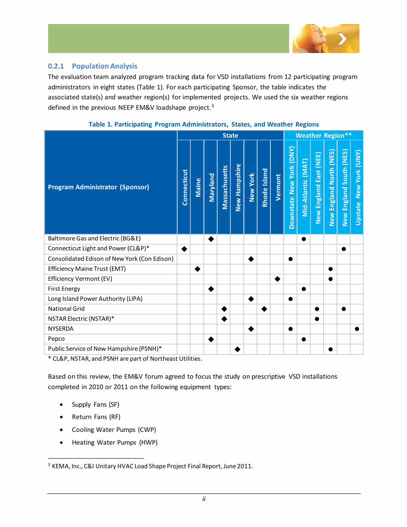
0.2.1 Population Analysis
The evaluation team analyzed program tracking data for VSD installations from 12 participating program
administrators in eight states (Table 1). For each participating Sponsor, the table indicates the
associated state(s) and weather region(s) for implemented projects. We used the six weather regions
defined in the previous NEEP EM&V loadshape project.3
Table 1. Participating Program Administrators, States, and Weather Regions
Program Administrator (Sponsor)
State Weather Region**
Co
nn
ecti
cut
Mai
ne
Mar
ylan
d
Mas
sach
use
tts
New
Ham
psh
ire
New
Yo
rk
Rh
od
e Is
lan
d
Ver
mo
nt
Do
wn
stat
e N
ew Y
ork
(D
NY
)
Mid
-Atl
anti
c (M
AT)
New
En
glan
d E
ast
(NEE
)
New
En
glan
d N
ort
h (
NES
)
New
En
glan
d S
ou
th (
NES
)
Up
stat
e N
ew Y
ork
(U
NY
)
Baltimore Gas and Electric (BG&E)
Connecticut Light and Power (CL&P)*
Consolidated Edison of New York (Con Edison)
Efficiency Maine Trust (EMT)
Efficiency Vermont (EV)
First Energy
Long Island Power Authority (LIPA)
National Grid
NSTAR Electric (NSTAR)*
NYSERDA
Pepco
Public Service of New Hampshire (PSNH)*
* CL&P, NSTAR, and PSNH are part of Northeast Utilities.
Based on this review, the EM&V forum agreed to focus the study on prescriptive VSD installations
completed in 2010 or 2011 on the following equipment types:
Supply Fans (SF)
Return Fans (RF)
Cooling Water Pumps (CWP)
Heating Water Pumps (HWP)
3 KEMA, Inc., C&I Unitary HVAC Load Shape Project Final Report, June 2011.

iii
Water Source Heat Pump Circulation Pumps (WHP)
These five equipment types represent the VSD installations with the largest annual energy savings
across the NEEP Sponsor territories.
0.2.2 Sampling
Due to the objectives to capture five equipment types and analyze regional differences, the desire to
represent each study Sponsor, and limited auxiliary data for the study population, the evaluation team
developed a unique multi-stage, multi-phase sampling strategy. We implemented this staged and
phased sampling approach to develop the study sample of VSD projects (tracked projects with VSD
installations) and units (specific VSD installations). This approach enabled the team to conduct targeted
sampling to pursue adequate representation for each Sponsor, weather region, and equipment type,
while ensuring that the sample was representative of the regional population of VSD installation within
each equipment type category.
Sampling Stages
We performed two stages of sampling because the only relevant auxiliary variables for the population
were project size (tracked annual energy savings) and weather region. Although the sampling objective
was to collect a representative sample of the five selected equipment types, the evaluation team could
not sample based on equipment type because some program tracking data did not include these data.
In the first stage, we sampled projects based on project size and weather region. In the second stage, we
sampled units within each sampled project to target the appropriate equipment type for this study.
Sampling Phases
Because the tracking data did not include equipment type information for all projects and some
equipment types were more prevalent than others, we performed multiple phases of sampling to
ensure adequate representation of all five selected equipment types in the study sample.
In the first phase, we sampled projects (with the sample size set to 50% of the total project sample size)
and then analyzed the distribution of equipment types from those Phase 1 projects. For subsequent
sampling phases, we minimized selection of the equipment types (SF and CWP) that were most common
in the previous sampling phases, to maximize selection of the less-common equipment types (RF, HWP,
and WHP).
0.2.3 Data Collection
The study required extensive data collection—including on-site data collection and long-term metering
for over 400 VSD installations—to support this study. Table 2 summarizes the primary and secondary
data collection activities we completed between June 2012 and September 2013.

iv
Table 2. Data Collection Activities
Activity Description
Primary Data
Sponsor Tracking
Data
The evaluation team collected and reviewed the tracking data for VSD installations completed
through the Sponsor’s programs. We used these data to define the study population and
design the study sample.
On-Site Survey
and Metering
Equipment Inspection and Survey
The evaluation team surveyed facility staff for sampled projects to collect information about
normal facility and equipment operation and baseline conditions. We used these data to
develop our models for both VSD and baseline loadshapes.
Metering
The team installed power-metering equipment on sampled units to measure the energy
consumption of VSD-controlled equipment throughout the year between August 2012 and
September 2013. We used these data to model the hourly operation and electric demand of
VSD-controlled units.
Secondary Data
Existing Savings
Values, Methods
or Assumptions
for VSDs
TRM Review
The team reviewed the existing savings methods and assumption in the Sponsors ’ Technical
Reference Manuals. We used this information to compare the results of our study to existing
savings claims.
Review of Existing VSD Savings Methods
The team reviewed common methods for estimating energy and demand savings from VSD
installations. We used this information to develop our baseline demand model.
Massachusetts Pre/Post Metering Study
The team reviewed the meter data and analysis results from the Massachusetts Pre/Post
Installation VSD Study. We used these data and findings to develop and verify our baseline
demand model.
Historical and
Actual Weather
Data
The team collected actual and TMY hourly weather data for the Northeast and Mid-Atlantic
weather regions. We used actual hourly data to examine relationships between VSD power
and ambient weather conditions. We applied those relationships to TMY data to predict VSD
power during typical weather years.
0.2.4 Data Analysis
The evaluation team used primary and secondary data to develop estimates of the savings loadshapes
and savings metrics for each sampled unit, based on models that use the hourly operation and power
schedules for the pre- and post-retrofit conditions as well as typical calendar year weather conditions.
We used these unit-level models to estimate savings loadshapes and metrics based on typical weather
year conditions.
Hourly Operating Schedule
The hourly operating schedule indicates the percentage of time in each hour of the year that we expect
the unit to operate. Taking into consideration factors such as operating season, operating schedules,

v
and unit type, we used our meter and survey data to develop the post-retrofit operating schedule for
each unit.
Due to limited information about pre-retrofit operation, we assumed that the pre-retrofit (baseline)
operating schedule was the same as the observed post-retrofit (VSD) operating schedule. Although we
confirmed that a VSD installation could change both the operating power and the operating hours of the
connected equipment, we determined through discussions with the NEEP Technical Committee that this
study would focus only on the savings achieved by power reductions resulting from the VSD installation.
Hourly VSD Power Model
We developed a VSD power model for each unit to estimate the electric demand required by the unit
when it operates with the connected VSD. We analyzed relationships between measured operating
power and four variables: operating season, day type, hour, and outdoor temperature. We used the
relationships to develop a set of hourly models for each unit that predict the unit’s hourly power
demand based on a typical calendar year weather.
Figure 1 shows an example of our hourly modeling approach for a unit that exhibited temperature
dependence. The first row shows the actual hourly VSD demand plotted by temperature for weekdays
and weekends. The second row shows our modeled hourly output for the same temperature data. In
each figure, the colors indicate the different hourly models.
Figure 1. Examples of Hourly Models for Temperature-Dependent Units
Metered Power
Modeled Power
vi
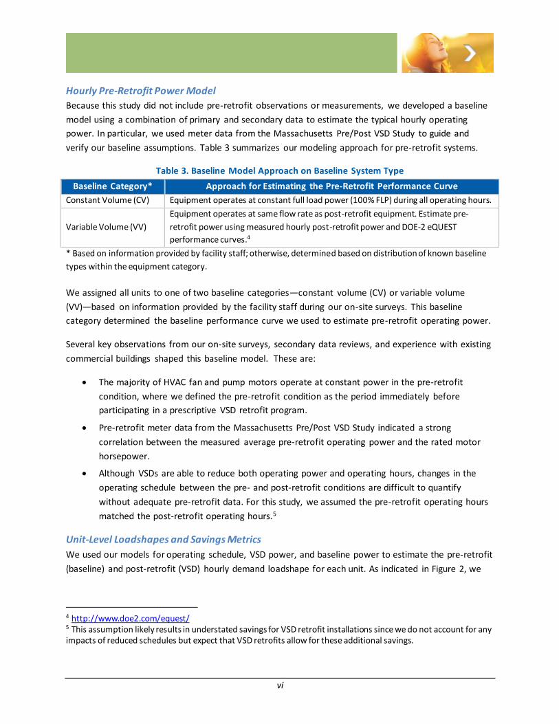
Hourly Pre-Retrofit Power Model
Because this study did not include pre-retrofit observations or measurements, we developed a baseline
model using a combination of primary and secondary data to estimate the typical hourly operating
power. In particular, we used meter data from the Massachusetts Pre/Post VSD Study to guide and
verify our baseline assumptions. Table 3 summarizes our modeling approach for pre-retrofit systems.
Table 3. Baseline Model Approach on Baseline System Type
Baseline Category* Approach for Estimating the Pre-Retrofit Performance Curve
Constant Volume (CV) Equipment operates at constant full load power (100% FLP) during all operating hours.
Variable Volume (VV)
Equipment operates at same flow rate as post-retrofit equipment. Estimate pre-
retrofit power using measured hourly post-retrofit power and DOE-2 eQUEST
performance curves.4
* Based on information provided by facility staff; otherwise, determined based on distribution of known baseline
types within the equipment category.
We assigned all units to one of two baseline categories—constant volume (CV) or variable volume
(VV)—based on information provided by the facility staff during our on-site surveys. This baseline
category determined the baseline performance curve we used to estimate pre-retrofit operating power.
Several key observations from our on-site surveys, secondary data reviews, and experience with existing
commercial buildings shaped this baseline model. These are:
The majority of HVAC fan and pump motors operate at constant power in the pre-retrofit
condition, where we defined the pre-retrofit condition as the period immediately before
participating in a prescriptive VSD retrofit program.
Pre-retrofit meter data from the Massachusetts Pre/Post VSD Study indicated a strong
correlation between the measured average pre-retrofit operating power and the rated motor
horsepower.
Although VSDs are able to reduce both operating power and operating hours, changes in the
operating schedule between the pre- and post-retrofit conditions are difficult to quantify
without adequate pre-retrofit data. For this study, we assumed the pre-retrofit operating hours
matched the post-retrofit operating hours.5
Unit-Level Loadshapes and Savings Metrics
We used our models for operating schedule, VSD power, and baseline power to estimate the pre-retrofit
(baseline) and post-retrofit (VSD) hourly demand loadshape for each unit. As indicated in Figure 2, we
4 http://www.doe2.com/equest/ 5 This assumption likely results in understated savings for VSD retrofit installations since we do not account for any impacts of reduced schedules but expect that VSD retrofits allow for these additional savings.
vii
calculated the savings loadshape by subtracting the hourly VSD loadshape from the hourly baseline
loadshape.
Figure 2. Calculation for the Unit-Level Savings Loadshape
We then used these unit-level savings loadshapes to calculate key savings metrics for each unit,
including annual energy and peak demand savings.
0.2.5 Aggregation Analysis
In a typical evaluation study, the evaluation team predefines the aggregation method based on the
sample design. This approach typically involves using sampling weights to aggregate the sampled unit
observations in order to produce a population-level estimate of the result. In this study, due to the
observed diversity in unit-level operating characteristics and distinct populations of temperature-
dependent and temperature-independent units, we developed and compared four different methods of
aggregation to analyze these differences in an aggregation analysis.
We worked with the NEEP Technical Committee to develop four methods as options for aggregating the
unit-level data into population results. Each method uses a different combination of unit-level data to
develop the population results, representing different assumptions that can be made about
differentiating or combining unit subpopulations across weather regions.
We developed a set of formulas to estimate the aggregated results for subpopulations of units (e.g.,
temperature-dependent supply fans in the Mid-Atlantic weather region) and to combine those
subpopulation results to obtain overall population results (e.g., supply fans in the Northeast). For each
aggregation method, we used these formulas to produce population-level savings estimates with
populations defined by equipment type and weather region.
In collaboration with the NEEP Technical Committee, we examined and compared the results of these
calculations to select the aggregation method that provides the most accurate and useful result to the
study Sponsors. We selected the aggregation method (Method D) that combines all unit data within
each equipment category across weather regions. We used aggregation Method D to develop a single
set of weighted average loadshapes and savings metrics for each equipment type that applies across the
northeast region.
Unit Pre-
Retrofit
Loadshape
Unit Post-
Retrofit
(VSD)
Loadshape
Unit
Savings
Loadshape

viii
0.3 Results Using the results of the aggregation analysis, the evaluation team combined the unit-level savings
results to develop average savings results for VSDs installed across the NEEP region. Although we
expected to observe significant regional differences in VSD performance, our observations and analysis
highlighted unexpected findings that guided our final approach and presentation of results. The final
study results represent the average per-horsepower savings achieved from VSD retrofits on key HVAC
systems in existing nonresidential buildings.
In this section, we describe the final study sample, our observations about the performance of the
sampled units, our findings about baseline systems, key assumptions that shape the analysis and results,
and our estimates of the average energy and peak demand savings achieved by VSD installations. We
follow the presentation of results with a discussion of the how the Sponsors may use the results for
future programs and the key findings that influenced the final analysis.
0.3.1 Final Sample
The savings results in this study rely on the primary data the evaluation team collected from the final
sample of VSD projects and units. Table 4 shows the final sample of metered units by equipment type
and weather region.
Table 4. Final Sample of Equipment Type by Weather Region
Equipment Type DNY MAT NEE NEN NES UNY Total Pct. of Total
Supply Fans (SF) 35 24 21 23 20 8 131 33%
Return Fans (RF) 9 15 13 17 4 2 60 15%
Cooling Water Pumps (CWP) 4 20 22 53 3 7 109 28%
Hot Water Pumps (HWP) 5 6 3 40 11 12 77 20%
Water Source Heat Pump
Circulation Pumps (WHP) 3 0 1 8 3 0 15 4%
Total 56 65 60 141 41 29 392 100%
Percent of Total 14% 17% 15% 36% 10% 7% 100% NA
Weather Regions: DNY = Downstate New York; MAT = Mid-Atlantic; NEE = New England East; NEN = New England North; NES = New England South; UNY = Upstate New York
The final sample includes 392 VSD installations across all weather regions and equipment types. We
stratified by weather region in our sampling approach, so that the number of sampled projects across
the weather regions would be representative of the distribution in the population. Due to our phased
sampling approach, the overall distribution of equipment types may not represent of the overall
population of prescriptive VSD installations (i.e., supply fans likely represent more than 33% of the
installations overall). However, within each equipment type category, the distribution of units across
weather regions likely represents the distribution in the population. We used sampling weights at both
the project and unit levels to account for any differences in the sampling and population distributions.

ix
Figure 3 shows the distribution of motor sizes in the final sample. In each figure, the x-axis shows the
range of motor sizes eligible for the study sample (0 to 200 horsepower) and the y-axis indicates the
percentage of motors in the sample for each motor size.
Figure 3. Distribution of Motor Sizes (motor hp) by Equipment Type
Supply Fans (SF)
Return Fans (RF)
Cooling
Water Pumps (CWP)
Hot Water
Pumps (HWP)
WSHP Circulation
Pumps (WHP)
Motor Size (hp)
To be consistent with the typical guidelines for prescriptive VSD incentives in the Sponsors’ programs,
we included all VSDs on motors up to 200 horsepower in the study population. We excluded units from
the sample based on motor size only if the motor was larger than 200 hp. Other than this exclusion of

x
large motors, this motor size distribution represents the overall population of prescriptive VSD
installations for each equipment type.
Figure 4 shows the distribution of building types in the final sample. The bars in the table indicate the
relative distribution of each building type compared to the others.
Figure 4. Distribution of Building Types in Final Sample
The evaluation team developed the list of 12 building types as part of the data collection protocols.
During the site visits, the evaluation team verified or determined the building type for each sampled site
and assigned each site to one of the 12 listed building types. We did not exclude any projects based on
building type, so we believe this distribution is representative the overall population distribution.
Although we expect building type to be an influential parameter in VSD performance, we could not
stratify the sample by building type due to limitations in the project scope and auxiliary data. In
addition, the diversity operating schedules and strategies across the sample suggests that building type
is not a reliable indicator of VSD performance.
0.3.2 Observed Variation in VSD Operation
Throughout the data collection and analysis activities, the evaluation team observed significant variation
in the operating patterns of sampled units. Figure 5 shows an example of the differences in operating
schedules (e.g., continuous operation vs. scheduled operation) and in operating power (e.g. , constant vs.
variable power).
Building Types Percent of Sample
Office 35%
Restaurant 0%
College/University (non-Residential) 20%
Industrial/Manufacturing 5%
Retail 2%
Hospital 8%
K-12 11%
Warehouse 1%
Grocery 0%
Multifamily/Dormitory 9%
Hotel/Motel/Lodging 4%
Other 7%

xi
Figure 5. Examples of Observed Variation in VSD Operation
Continuous (24/7) Operation Scheduled Operation
Constant Power
Variable
Power
In addition to differences in equipment schedules and power settings, factors such as motor
configuration and seasonality increased the variation in our models of VSD demand and savings. We
used all of these factors to develop annual estimates of energy and demand savings at the unit level.
0.3.3 Estimates of Baseline Operation
Because this study focused on post-installation operation of equipment with VSDs, we relied on facility
staff to describe pre-retrofit operation for all sampled. We used this survey information to develop an
initial distribution of baseline categories, then re-assigned any VSD or unknown baseline categories to
develop the adjusted distribution for the savings analysis. Table 5 shows the initial and adjusted
distributions of baseline categories for each equipment type.
Table 5. Reported Baseline (Pre-Retrofit) Category
Baseline Category SF RF CWP HWP WHP All
sample n = 131 n = 60 n = 109 n = 77 n = 15 n = 392
Initial Distribution
Constant volume (CV) 31% 42% 35% 25% 40% 33%
Variable volume (VV) 1% 6% 0% 0% 0% 2%
Variable speed drive* 1% 2% 0% 0% 0% 1%
Unknown** 66% 50% 65% 75% 60% 65%
Adjusted Distribution***
Constant volume 97% 92% 100% 100% 100% 98%
Variable volume 3% 8% 0% 0% 0% 2% * Based on discussions with the NEEP Technical Committee, we reassigned VSD baselines to either CV or VV. Since VSDs are not an eligible baseline for any Sponsor programs, the team elected to remove this baseline category from the final analysis. ** The high percentage of units with unknown baselines is likely due to the elapsed time (minimum of one year) since the site installed the VSDs. *** We assigned all equipment with VSD or unknown baselines by randomly assigning the unit to a CV or VV baseline based on the probably of those baselines occurring in the initial, or “known” distribution.

xii
The initial distribution shows that facility staff could not define the baseline system for almost two-
thirds of the studied units. This inability to report on the baseline conditions was prevalent for the
majority of sampled units across all equipment types. This is not surprising for a data collection effort
conducted a minimum of one year after the customer installed the VSD equipment.
Among those staff members who could recall the baseline system type and operation, the majority
indicated that the equipment operated at constant speed and power before the customer installed the
rebated VSDs. Among these, some staff indicated that although variable volume equipment existed, the
site was installing VSDs because the existing variable volume equipment was not in working condition.
We classified these cases in the constant volume category.
To estimate the adjusted distributions, the evaluation team re-assigned the baseline category for units
with an unknown or VSD baseline in the initial distribution based on the observed distribution of CV and
VV baselines among the known baseline categories within each equipment group. In other words, we
randomly assigned each “unknown” or “VSD” baseline from the initial distribution to either the CV or VV
baseline category using the probability of CV or VV from the initial baselines.
The final distribution demonstrates our estimate that almost all systems operated as constant volume
prior to the VSD retrofit. Although contrary to many TRM approaches that assume a higher fraction of
variable volume baselines, we confirmed through multiple discussions with the NEEP Technical
Committee and building commissioning engineers that this high percentage of systems operating at
constant volume is consistent with field observations across existing buildings and with the pre-
installation findings from the MA VSD Pre/Post study. The following points support this finding:
The CV baseline category includes systems that were designed as VV but operate as CV, because
of improperly operating controls, broken equipment, etc.
The program population of buildings does not include the full C&I building stock. Rather, the
population includes only those existing buildings that participated in one of the Sponsors’ VSD
retrofit programs. Existing buildings with working variable volume systems are less likely to
participate in the programs since there is no need to replace the working VV equipment.
Eligibility requirements for several Sponsor VSD programs do not allow rebates for existing VV
systems in working condition. This filter likely further reduces the number VV baselines among
the participant population.
Our commissioning engineers agree that based on their experience in existing buildings, it is
becoming less and less common to see non-VSD VV systems in working condition. Frequently,
they will find evidence that these VV systems were part of the original design, but noted that
they are often not working. For example, we see guide vanes that are locked in place so they
effectively operate as constant volume systems.
For pumping systems, pumps without VSD controls are typically constant volume by design.
There are systems that use variable volume distribution in the building (e.g. two-way valves at

xiii
the coils), but they are typically configured using bypass valves at the plant so the primary loop
pump would still operate at full, constant volume.
Although the sample was small, the pre-retrofit metering results from the Massachusetts
Pre/Post VSD study are consistent with these assumptions. For that study, the field team
observed and metered the equipment prior to when the VSD was installed. They identified a
couple systems that were designed as VV, but the meter data showed constant power on those
fans.
0.3.4 Key Assumptions
Based on our findings in both the primary and secondary data and the need to develop a standard
approach to estimate savings in this study, we developed several key assumptions to guide our savings
analysis. In collaboration with NEEP’s EM&V Technical Committee, we applied the following key
assumptions in this study:
Pre-Retrofit Operating Power. Due to the post-installation focus of the study, the evaluation
team could not measure pre-retrofit operating power. We modeled pre-retrofit power based on
a combination of the unit-rated horsepower, metered post-installation power, on-site survey
data about the pre-retrofit condition, and results of the Massachusetts Pre/Post Metering Study.
Pre-Retrofit Schedule. Due to the post-installation focus of the study, the evaluation team could
not monitor the pre-retrofit operating schedule. We assumed the pre-retrofit operating
schedule was the same as the post-retrofit operating schedule.
Units with Baseline VSD. A small number of interviewed on-site staff indicated that the new
VSDs replaced existing VSDs. Since replacement of existing VSDs is not eligible in the Sponsor’s
programs and an attribution study would likely capture these occurrences, we assigned a new
baseline category for these units based on the observed proportion of baseline categories for
the remaining units.
Non-Operating Units. Our metering and on-site data collection indicated 52 of 392 (<14%) units
that have low operating hours due to rotating, lead-lag, or back-up control strategies. We
retained these units in the study sample to represent these occurrences as we observed them in
the study population.
0.3.5 Savings Metrics
The team used the unit-level savings results to estimate average savings metrics for the population of
prescriptive VSD projects installed through the Sponsor’s energy-efficiency programs. Based on key
observations and findings during the data collection and analysis tasks, we produced a single set of
savings results for each equipment type to reflect the average savings across all northeast weather
regions. The northeast average results account for the diversity of motor sizes, building types, HVAC
loads, and control strategies observed in the study sample.
The following tables describe the estimated savings for each equipment type. In addition to the per-
horsepower savings values, the tables show the relative precision for each result at both 90% and 80%

xiv
confidence levels. Although the study aimed to achieve 10% relative precision at 90% confidence for the
key savings metrics, the variability of performance among sampled units resulted in higher relative
precision values.
Table 6 shows the estimated annual energy savings per horsepower for units across the NEEP region.
We present the annual energy savings in units of kWh per hp.
Table 6. Annual Energy Savings per Unit Horsepower
Equipment Type kWh/hp RP @ 90% RP @ 80%
Supply Fans 2,033 23.5% 18.3%
Return Fans 1,788 13.8% 10.8%
Cooling Water Pumps 1,633 17.7% 13.8%
Hot Water Pumps 1,548 18.4% 14.3%
WSHP Circulation Pumps 2,562 12.8% 10.0%
* Results apply for all units across the Northeast Mid-Atlantic states.
Table 7 shows the estimated demand reduction value for the ISO-NE summer and winter on-peak
periods.6 We present these summer demand savings in units of kW per hp.
Table 7. ISO-NE Summer and Winter On-Peak Demand Savings per Unit Horsepower
Equipment Type ISO-NE Summer On-Peak ISO-NE Winter On-Peak
kW/hp RP @ 90% RP @ 80% kW/hp RP @ 90% RP @ 80%
Supply Fans 0.288 18.8% 14.6% 0.265 21.5% 16.7%
Return Fans 0.302 11.9% 9.3% 0.274 15.3% 11.9%
Cooling Water Pumps 0.183 16.7% 13.0% 0.194 18.2% 14.1%
Hot Water Pumps 0.096 34.1% 26.5% 0.221 20.7% 16.1%
WSHP Circulation Pumps 0.229 22.0% 17.1% 0.297 12.4% 9.7%
* Results apply for all units across the Northeast and Mid-Atlantic states.
Table 8 shows the estimated demand reduction value for the PJM summer peak period.7 We present
these summer demand savings in units of kW per hp.
6 The ISO-NE on-peak summer demand reduction is the expected average demand reduction between the hours 1 p.m. and 5 p.m. on non-holiday weekdays in June, July, and August. The ISO-NE on-peak winter demand reduction is defined as the average demand reduction between the hours of 5 p.m. and 7 p.m. on non-holiday weekdays in December and January. 7 The PJM summer peak demand is the expected average demand reduction during the hours 2 p.m. and 6 p.m. on non-holiday weekdays in June, July, and August.

xv
Table 8. PJM Summer Peak Demand Savings per Unit Horsepower
Equipment Type kW/hp RP @ 90% RP @ 80%
Supply Fans 0.286 19.0% 14.8%
Return Fans 0.297 12.4% 9.7%
Cooling Water Pumps 0.185 16.7% 13.0%
Hot Water Pumps 0.096 34.3% 26.7%
WSHP Circulation Pumps 0.234 20.6% 16.0%
* Results apply for all units across the Northeast and Mid-Atlantic states.
The team compared the study results with the estimated savings assumptions from the Massachusetts,
Mid-Atlantic, and New York Technical Reference Manuals and to the results of the Massachusetts
Pre/Post VSD study. For each parameter, the savings results generally fall within the expected range of
savings.
0.3.6 Key Findings that Explain the Results
We uncovered multiple important findings that guided our analysis approach and dictated our
recommendation for a single set of savings results averaged across the NEEP region.
Variable speed drives frequently operate at constant speed.
Our on-site observations and metering data showed that customers operated at least one third of VSD-
controlled motors at a constant speed (typically less than full speed) during the nine- to 12-month data
collection period. Similarly, the Massachusetts Pre/Post VSD Study found that customers operated more
than two-thirds of the metered VSDs at constant speed. When we discussed this operating strategy
during our on-site interviews,8 some facility operators indicated that they intended this constant speed
operation while others indicated that they had not fully commissioned the VSD equipment. Although we
expect VSDs to vary the motor speed depending on load conditions, the observed constant speed
operation may result in higher energy savings during peak demand periods compared to when standard
savings assumptions that VSD-controlled motors operate at or close to full speed during peak
conditions.
Operators may select constant speed operation over variable speed operation.
Although we expect operators to use new variable speed drives to vary the operating speed of the
motor, we found that it is not uncommon for operators to choose to operate the motor at a constant
speed setting. Through discussions with facility staff in this study and our building commissioning
engineers, we identified several reasons an operator may choose to use a VSD to operate a motor at
constant speed:
8 We asked these questions during removals at the end of our data collection period to minimize any influence on the facility’s typical operation.

xvi
Operators may use a VSD to dial in on a reduced constant flow requirements. Reduced constant
flow could also be achieved by using a valve or damper to throttle the flow or for certain
pumping applications modifications could be made to the pump impellers. Compared to the
throttling option, the VSD substantially reduces power requirements, energy consumption, and
energy costs. Compared to the impeller modification option, the VSD allows the operator to
keep the existing equipment in place and retains the flexibility of increasing speed (and capacity)
if needed in the future.
Operators may forgo the cost of implementing the controls for variable speed operation and
instead settle on a reduced constant speed that is acceptable. Implementing controls may
require installing new flow or pressure sensors, connecting those sensors and the VSD to a
central EMS, programming controls sequences, and commissioning the system to ensure that
the controls work correctly. Due to the cost and time requirements, operators may prefer to
operate the equipment at a constant speed that meets the generally meets flow
requirements. This constant speed may be higher than the necessary for periods of low load,
but still reduces energy consumption and costs compared to constant speed. The installation of
the VSD allows them to take advantage of further operational modifications if the controls are
updated in the future.
Variable speed drive performance often does not track outside temperature.
In addition to a large percentage of VSDs that operated at a constant speed setting (discussed above),
our unit-level data analysis demonstrated that the operating power for more than half of the units did
not correlate with ambient temperature. Unlike larger equipment that operates to meet whole-building
HVAC loads, internal variables such as occupancy or occupant activity may be more influential to VSD
performance than external variables such as ambient temperature.
The savings estimates for each weather region are similar and similarly diverse.
In our aggregation analysis, we calculated average savings for each weather region and compared
savings estimates between regions as well as to the average across all regions combined (NEEP region).
The comparison showed that the confidence intervals for the regions overlap in most cases, suggesting
that the average results are not very different from region to region. The confidence interval for the
combined NEEP region covered a range that lies within the other regional intervals but provided a
narrower margin of error around the mean. Further, we found that the variation in operation was
similar from region to region, which provided another indication that regional differences were small.
Due to these findings, we present average savings across all six weather regions.
Most pre-retrofit equipment operates at constant power.
The evaluation team’s on-site survey and secondary data review indicated that a majority of pre-retrofit
equipment operated at constant power. As indicated in Table 5, we modeled 98% of the pre-retrofit
systems at constant power (after removing several occurrences of VSD baselines from the sample).
Although standard VSD assumptions often model other variable flow systems as the baseline for VSD
retrofit project, our research suggests that even when these variable flow systems exist they are not in

xvii
working condition. Our research is supported by the Massachusetts Pre/Post VSD Study, which
demonstrated constant power operation for 100% of the pre-retrofit systems.
0.3.7 Application of Results
Implementers in the Northeast and Mid-Atlantic states may use these results to estimate the savings for
VSD installations that meet the following characteristics:
The VSD is retrofitted on HVAC equipment in an existing nonresidential building and does not
replace an existing, working VSD.
The VSD controls a motor no larger than 200 horsepower.
The VSD controls a motor driving one of these equipment types: (1) supply fans, (2) return fans,
(3) chilled water plant distribution pumps, (4) hot water distribution pumps, and (5) water
source heat pump distribution pumps.
The controlled equipment serves an HVAC load.
When using these results, the implementer should calculate the desired savings parameter by
multiplying the rated horsepower of the motor or total horsepower of the population of motors by the
appropriate savings factor from the tables above. For example, to estimate the annual energy savings
for a VSD retrofit project on a 50-hp supply fan, the implementer should multiply 50 (the rated
horsepower of the existing motor) by the appropriate savings factor from Table 6. Similarly, the Sponsor
may estimate the ISO-NE on-peak demand reduction by multiplying 50 (the rated horsepower) by the
appropriate demand savings factor from Table 7.
Dissimilar to many TRM savings approaches that provide savings factors by building type or that use
engineering algorithms to estimate savings using project-specific input parameters, the results of this
study are averaged savings that account for the varied performance of VSD installations across building
types and weather regions in the Northeast and mid-Atlantic states. This study does not deny the
influence of building operating hours or ambient temperature on VSD performance; however, the
diversity of equipment performance demonstrated in this study indicates that these two variables are
not reliable predictors for VSD performance. As discussed in this report, many other factors such as
equipment operating schedules, motor configuration, and VSD control strategy also influence VSD
performance and savings estimates.
These study results are based on direct and long-term measurements of nearly 400 VSD installations and
account for the diversity of motor sizes, building types, HVAC loads, and operating strategies, and
seasonal differences across the northeast. The results also account for recent, measured findings about
pre-retrofit performance.
0.4 Recommendations The evaluation team offers the following recommendations for implementers and evaluators of VSD
projects to improve the energy savings of VSD installations and effectiveness of VSD programs.

xviii
Recommendations for Implementers
Continue to promote the installation of VSD on existing equipment.
VSD retrofit projects are achieving significant energy and demand savings across the
Northeast and Mid-Atlantic regions.
To ensure VSDs operate as intended to achieve energy and demand savings, Program
Administrators should integrate VSD control and commissioning requirements into program
implementation activities. Application forms should require specification of the intended control
strategy, and post-installation inspection should include verification of commissioned VSD
control sequences.
We observed during the site visits and in our reviews of the metered data that many
customers operate their VSDs at constant speed. In some cases, customers intend to
operate VSDs at constant speed, but for many customers this constant-speed operation is
due to incomplete project commissioning. In addition, we found that a larger percentage of
VSDs operated at constant power in the Massachusetts Pre/Post VSD Study (conducted
immediately before and after VSD installation) compared to the NEEP study (conducted at
least one year after installation). We assume that the lower percentage of constant-speed
units observed in this study is due to the longer period of elapsed time after the VSD
installation, which allowed more customers to complete commissioning.
As VSDs saturate the existing building stock, the Program Administrators should take more care
in screening project eligibility.
For several sampled projects, the rebated VSD units replaced existing VSD units at the end
of their useful lives. Although we did not include those baseline occurrences in this study,
these observations are evidence of projects’ receiving program incentives despite
ineligibility.
To support future evaluation efforts, the Program Administrators should add pre-retrofit data
collection requirements to program application forms. At minimum, the PAs should require
customers to specify the baseline system type and working condition of that system and
operating schedule for the baseline equipment.
Information about baseline operation is limited in Sponsor tracking data and difficult to
collect after customers complete VSD projects. Since baseline operation is a critical
component for estimating energy and peak demand savings, it is important for the programs
to record the working condition of baseline systems as well as the existing operating
strategy and schedule.
Recommendations for Evaluators
The timing of the post-installation inspection and metering is important. Our findings suggest
the customers may take a year or longer installing the VSD to set up the controls and fully
commission the system. Performing evaluation activities within a year of installation will provide

xix
accurate first-year results, but may not accurately reflect VSD performance in the following
years.
When metering VSD power for energy analyses, the evaluator should examine seasonal
operation defined for each facility. Seasons may be associated with changes in equipment
purpose (e.g., heating or cooling), occupancy patterns (e.g., academic year vs. vacation periods),
or other parameter such as control strategy (e.g., constant vs. variable speed).
Customers use HVAC motors differently throughout the year. This is especially true for
equipment in seasonal facilities and for equipment that serve both heating and cooling
loads.


1
1 Introduction
This study is the third in a series of savings loadshape studies focused on efficient technologies
implemented through the energy-efficiency programs of NEEP’s Sponsors. This loadshape study targets
the annual, peak, and hourly electric demand savings achieved by variable speed drives (VSDs) installed
on existing heating, ventilation, and air conditioning (HVAC) equipment in commercial buildings
throughout the Northeast and Mid-Atlantic states, including Maryland, Maine, Massachusetts,
Connecticut, Vermont, New Hampshire, and Rhode Island, and New York.
1.1 NEEP EM&V Forum The Northeast Energy Efficiency Partnerships (NEEP) is a nonprofit organization established to promote
energy-efficiency throughout the Northeast and Mid-Atlantic.9 NEEP created the Evaluation,
Measurement, and Verification (EM&V) Forum in 2008 “to support the development and use of
consistent protocols to evaluate, measure, verify, and report the savings, costs, and emission impacts of
energy efficiency and other demand-side resources.”
In particular, the EM&V Forum facilitates joint research and evaluation by pooling funds from multiple
Sponsors to conduct large-scale research studies such as the loadshape series.10 These studies provide
robust estimates of the energy and demand savings achieved by demand side resources the Northeast.
Table 9 shows Sponsors of the EM&V Forum and indicates the states included in this VSD loadshape
project.
Table 9. EM&V Forum Sponsors and VSD Study Participants
State Sponsor Study
Participant* Connecticut CT Energy Efficiency Fund
District of Columbia District Dept. of the Environment
Maine (2012) Efficiency Maine Trust
Maryland
Maryland Energy Administration
EmPOWER Maryland Utilities (PHI/Pepco, Delmarva, SMECO, First
Energy, Baltimore Gas & Electric)
Massachusetts
Cape Light Compact
National Grid
NSTAR
Unitil
Western Massachusetts Electric Company
9 www.neep.org 10 The NEEP EM&V forum has completed two loadshape studies to date: The Commercial Lighting Loadshape Study (completed in 2011) and the Unitary AC Loadshape Study (completed in 2012).

2
State Sponsor Study
Participant*
New Hampshire
NH Electric Co-op
Public Service New Hampshire
Unitil
New York
Long Island Power Authority
New York Power Authority
New York State Energy Research and Development Authority
Rhode Island National Grid
Vermont Department of Public Service
* Participants are Program Administrators that provided data for the study population of VSD installations.
1.2 Project Objectives and Scope The objective of the NEEP VSD Loadshape study is to develop estimates of the annual, peak, and hourly
demand savings of achieved variable speed drive (VSD) installations on existing HVAC equipment in
commercial buildings. In the early stages of this project, the Subcommittee agreed to focus on the five
equipment type categories that make up the majority of annual energy savings from VSD installations
across the Sponsors’ programs:
Supply fans
Return fans
Cooling water pumps
Heating hot water pumps
Water source heat pump circulation pumps.
The study uses both primary data—direct power metering and data collection for a sample of VSD
installations across the Sponsors’ programs—and secondary data to establish the hourly savings
loadshapes for each of these selected equipment type categories.
1.3 Definitions In Table 10, we provide definitions for terms critical to understanding the sampling, data collection,
and/or analysis methods we used for this study.
Table 10. Definition of Terms
Term Definition
Variable Speed
Drive (VSD)
Variable speed drives control the operating speed of connected motors based on
programmed control strategies.
HVAC Heating, Ventilation, and Air Conditioning; in this study, we focus on VSDs installed on or
equipment that serve HVAC loads in existing nonresidential buildings.

3
Term Definition
Loadshape
A loadshape describes the hourly electricity demand for all 8,760 hours in a year. In this
study, we calculate demand loadshapes to model the hourly electric demand of HVAC
equipment with or without VSDs. Similarly, we calculate savings loadshapes to model the
expected hourly demand reduction achieved by VSD-controlled equipment compared to the
pre-retrofit or baseline condition.
Equipment Type
Equipment type refers to the categories of commercial HVAC equipment. In this study, we
focus on these five equipment type: supply fans, return fans, cooling water pumps, heating
hot water pumps, and water source heat pump distribution pumps.
Project
Project refers to an activity completed by a participant in one of the Sponsors’ programs and
tracked in the Sponsor’s database, in which one or more VSDs were installed. All projects in
the study sample had at least one VSD installation on one of the five defined equipment
types.
Unit
A unit refers to a unique VSD installation as part of a VSD project. All units in the study
sample involved power metering for VSD-controlled equipment from one of the five selected
equipment types.
Sample Phase
We performed multiple phases of sampling in order to improve the distribution of equipment
types in the study sample. Each sampling phase has a different condition set for the eligible
population, in order to target specific equipment types.
Sample Stage
We performed two stages of sampling within each sample phase. The first stage involved
sampling projects based on project size and weather region. The second stage involved
sampling the units within a sampled project for power metering.
Target Sample The target sample describes the ideal sample of projects and units developed in the sample
strategy and used to guide the sample draw.
Study Sample
The study sample is the collection of projects and units included in the analysis. Differences
between the target and study samples may be due to (1) small populations of projects in
some strata and weather regions, (2) inability to control for equipment type in the sample
draw, and (3) differences between expected and actual units for given project.
Operating Power
We use the term operating power to describe the measured or estimated power demand
from the motor during periods of operation. For example, in our analysis of metered
operating power, we examine the measured power only during periods when the motor is
operating.
Primary/Lead
Units
Primary units operate as the primary, or lead, equipment to serve the designated load. When
there is a call for heating, cooling, or ventilation, the primary unit will respond to meet the
load requirements.
Lag Units
Lag units assist primary, or lead, equipment when the lead equipment reaches its maximum
capacity or a maximum setting. In these scenarios, the lag units will respond to serve load any
load beyond what is served by the lead unit. Because the primary equipment usually serves
the full HVAC load, lag units typically only operate when the loads are unusually high.
Rotating Units
Rotating units operate in a team of similar units to serve the same load. Facility operators
rotate units to lengthen the lifetime of equipment and to provide redundancy in case of
failure. Since rotating units take turns serving the designated load, each unit operates for
only a fraction of the team’s overall schedule.

4
Term Definition
Back-up Units
Back-up units rarely operate and are in place to provide redundancy for primary or rotating
units. Back-up units typically operate only when the other equipment malfunctions or is
turned off for regular maintenance activities.
Weather Regions
We defined the following six weather regions for this study: DNY = Downstate New York; MAT
= Mid-Atlantic; NEE = New England East; NEN = New England North; NES = New England
South; UNY = Upstate New York
1.4 Acknowledgements Many parties contributed to the design and execution of this loadshape study. First, we thank the NEEP
EM&V Forum for engaging the region in these complex loadshape projects and organizing the many
stakeholders throughout the project.
We thank the Forum Sponsors and Loadshape Subcommittee members for recognizing and contributing
to this important research. At each stage of the project, Sponsors and subcommittee members provided
critical project data, reviewed project deliverables, and participated in project status meetings. We
thank the subcommittee members for their diligence in responding to data requests and for
contributing thoughtful feedback during each phase of the project.
The subcommittee members include: Cheryl Hindes, Mary Straub, and Sheldon Switzer from BG&E;
Kristin Graves, Michael Ihesiaba, and Mahdi Jawad from Con Edison; Kristy Fleischmann from
Constellation Energy; Matt Quirk and Chris Siebens from First Energy; Bill Blake and Whitney Brougher
from National Grid; Dave Bebrin, Tom Belair, Geoff Embree, Monica Kachru, Gary LaCasse, Joe Swift, and
David Weber from Northeast Utilities (including CL&P, NSTAR, and WEMCo); Marilyn Brown and Mary
Cahill from NYPA; Deborah Pickett from NYSEG; Judeen Byrne, Tracey DiSimone, Victoria Engel-Fowles,
and Ed Kear from NYSERDA; David Sneeringer from Pepco; Paul Gray from United Illuminating; Mary
Downes from Unitil; Bill Fischer and Nicola Janjic from VEIC; Jim Cunningham and Leszek Stachow from
the NH PUC; Niko Dietsch from the EPA; Taresa Lawrence from the District of Columbia Energy Office;
Amanda Kloid and James Leyko from the Maryland PSC; Arthur Maniaci from the New York ISO; Ralph
Prahl from the Massachusetts EEAC; Allison Reilly from NESCAUM; Jennifer Chiodo from CX-Associates
(Massachusetts Energy Efficiency Advisory Council); Scott Dimetrosky from Apex Analytics (Connecticut
Energy Efficiency Board); Colin High from Resource Systems Group, Inc. ; Lori Lewis from Analytical
Evaluation Consultants (Connecticut Energy Efficiency Board); Lisa Skumatz from SERA, Inc.
(representing Connecticut Energy Efficiency Board); Doug Hurley from Synapse-Energy; and Julie
Michals, Elizabeth Titus, Cecily McChalicher, and Danielle Wilson from the NEEP EM&V Forum.
Finally, we thank the members of the NEEP Loadshape Technical Committee–Elizabeth Titus, David
Jacobson, and Steve Waite–who participated in many long discussions and contributed insightful
questions, feedback, and recommendations throughout the project.

5
2 Methods
The evaluation team conducted this VSD loadshape study in the five key tasks described in Figure 6. This
progression of tasks is similar to the previous loadshape studies and other EM&V research. However,
the specific methods within each task are uniquely complex due to limitations in the program tracking
data, elapsed time since the project completion, and variation in the operation of VSDs throughout the
study sample. In this section and referenced Appendices, we describe the methods for each analysis
task including our observations and key assumptions.
Figure 6. Key Tasks for Loadshape Analysis
2.1 Sample Design For this study, the evaluation team developed a unique sampling strategy to account for varying levels
of available tracking data from the Sponsors, limited information about the equipment types in the
population of projects, and expected variation between weather regions and Sponsors.
In this first task, we reviewed the Sponsors’ tracking data, designed the sample framework, and created
the sample. This strategy is documented in the memorandum “VSD Loadshape Project – Proposed
Sampling Strategy, Updated,” dated August 2, 2012.
2.1.1 Analysis of Sponsor Tracking Data
After the project kick-off meeting, the evaluation team submitted a data request to the NEEP EM&V
Technical Committee and study Sponsors. We received participation records from 12 Sponsors. These
data included 3,845 lines accounting for 2,109 unique projects completed between 2009 and 2012.
Based on our review of these data and follow-up discussions with specific Sponsors, we developed a set
of criteria to further define the dataset. We excluded all projects that met any of the following criteria:
The project was completed in or before 2009.
The project was not yet completed.

6
The customer installed the VSD on equipment serving process loads or on chiller compressors.
The project was new construction or major renovation.
The project was part of a NYSERDA custom program.
These criteria reduced the qualified sampling population to 2,798 unique data lines, representing 1,582
unique projects. It is important to note that this qualified population may include some unqualified
projects, since we could not remove projects for which we did not have complete tracking data.
Table 11 summarizes the tracking data provided by each Sponsor, including whether each data type was
available in the Sponsor tracking data. The last column indicates the data types available across all
Sponsor data.
Table 11. Tracking Data Characteristics by Sponsor
Data Type
Effi
cien
cy M
ain
e
PSN
H
Effi
cien
cy V
erm
on
t
Nat
ion
al G
rid
NST
AR
CL&
P
Co
n E
dis
on
NYS
ERD
A
LIP
A
Pep
co
Firs
t En
ergy
BG
&E
All
Project Energy Savings
Project Demand Savings
Measure Level Energy
Savings ○
Project Type (New/Retrofit) ○ ○ Prescriptive Projects Custom Projects ○ Equipment Type ○ ○ ○ ○ ○ Base Case Control Type ○ Building Type ○ ○ ○ ○ ○ ○ 2010 Projects ○ 2011 Projects
2012 Projects ○
Indicates that the Sponsor provided information on almost all projects. ○ indicates that the Sponsor provided information on some projects. A blank cell indicates that these data were not available.
The last column in Table 11 indicates that only four data types were consistently available in all
Sponsors’ tracking data: project energy savings, project demand savings, prescriptive projects, and 2011
projects. Therefore, when comparing data to determine the relative impact of any equipment type,
building type, or Sponsor, we limited our review to only data from 2011 projects.

7
The following tables summarize 2011 installations by state, sponsor, equipment type, and building
type.
Table 12. 2011 Records by State
State 2011 Data Lines 2011 Annual Energy
Savings (kWh)
Percent of 2011 Annual
Energy Savings
New York 534 52,094,873 58.70%
Massachusetts 269 16,863,715 19.00%
Maryland 152 10,875,541 12.25%
Connecticut 65 3,344,469 3.77%
Rhode Island 36 2,301,688 2.59%
Maine 107 1,566,232 1.76%
New Hampshire 18 973,232 1.10%
Vermont 39 731,616 0.82%
Total 1,220 88,751,364 100.00%
Table 13. 2011 Records by Sponsor
Sponsor 2011 Data Lines 2011 Annual Energy
Savings (kWh) Percent of 2011 Annual
Energy Savings
Consolidated Edison 126 29,675,457 33.44%
NYSERDA 370 21,214,476 23.90%
Northeast Utilities (NSTAR) 161 10,128,360 11.41%
National Grid 146 9,454,766 10.65%
BG&E 120 6,742,301 7.60%
CL&P 65 3,344,469 3.77%
Pepco 21 3,093,340 3.49%
Efficiency Maine 107 1,566,232 1.76%
LIPA 38 1,204,939 1.36%
FirstEnergy 11 1,039,900 1.17%
Efficiency Vermont 39 731,616 0.82%
PSNH 16 555,508 0.63%
Total 1,220 88,751,364 100.00%

8
Table 14. 2011 Records by Equipment Type
Equipment Type 2011 Data
Lines
2011 Annual Energy
Savings (kWh)
Percent of 2011 Annual
Energy Savings
All Excluding Unknowns UNKNOWN* 444 24,695,866 27.83% NA
Cooling Water Pump** 148 16,711,456 18.83% 26.09%
Supply Air Fan 207 14,400,588 16.23% 22.48%
Fans, All Types*** 40 11,496,292 12.95% 17.95%
Water Source Heat Pump
Circulation Pump 38 3,848,103 4.34% 6.01%
Hot Water Pump 89 3,674,750 4.14% 5.74%
Boiler Feedwater Pump 37 2,888,901 3.26% 4.51%
Cooling Tower Fan 64 2,520,766 2.84% 3.94%
Pump, All Types*** 10 2,443,487 2.75% 3.81%
Building Exhaust Fan 50 2,436,508 2.75% 3.80%
Return Air Fan 71 1,996,261 2.25% 3.12%
Make-Up Air Fan 20 1,559,276 1.76% 2.43%
Boiler Draft Fan 2 79,111 0.09% 0.12%
* We assigned the unknown classification in cases for which the equipment type was not available.
** Cooling Water Pumps includes Chilled Water Pumps and Condenser Water Pumps. Some sponsors separate
these two technologies while others do not.
*** We used the “Fans, All Types” or “Pumps, All Types” classifications in cases for which (1) we knew the record
corresponded to a fan or pump installation, but did not know the specific type, or (2) multiple fans or mult iple
pumps of different types were within one record.
Table 15. 2011 Records by Building Type
Building Type* 2011 Data
Lines
2011 Annual Energy
Savings (kWh)
Percent of 2011 Annual Energy
Savings Office 238 37,051,892 41.75%
Manufacturing 161 11,160,532 12.58%
College 151 6,760,255 7.62%
Other 92 5,303,072 5.98%
Hospital 96 5,280,259 5.95%
UNKNOWN 90 4,276,818 4.82%
Education 125 3,907,962 4.40%
Hotel 38 3,652,553 4.12%
Retail 43 2,834,414 3.19%
Multifamily 35 2,204,420 2.48%
Health 43 2,062,459 2.32%
Water Supply or Treatment 14 1,080,205 1.22%

9
Building Type* 2011 Data
Lines 2011 Annual Energy
Savings (kWh)
Percent of 2011
Annual Energy Savings
Government 28 939,441 1.06%
Amusement 10 560,935 0.63%
Warehouse 10 457,530 0.52%
Institutional 1 223,832 0.25%
Assembly 14 223,213 0.25%
Commercial 8 147,813 0.17%
Mixed 8 137,325 0.15%
Laboratory 1 122,100 0.14%
Religious 1 96,954 0.11%
Restaurant 4 81,766 0.09%
Business 3 67,200 0.08%
Museum 2 51,480 0.06%
Automotive 2 24,520 0.03%
Misc. 1 23,296 0.03%
Grocery 1 19,121 0.02%
* The team classified building types based only on the text records in the Sponsor tracking data; we did not
reference SIC or NAICS codes for this stage of the project.
** It is unknown at this time if the VFD installations within each building type are serving HVAC equipment or
manufacturing equipment. If one of these projects is sampled and the installation is determined to be serving
manufacturing equipment, the sample point will be replaced.
The evaluation team made the following conclusions based on this review of the Sponsors’ 2011 VSD
projects:
Random sampling would result in bias toward the Sponsors that provided more years of data.
Furthermore, given that 88% of the stated savings occur within five service territories, the
evaluation team must take additional steps to ensure that all Sponsors are represented in the
study and that the results are applicable to the programs offered by each Sponsor.
Our framework used both weather region and size category as stratification variables to
reduce this bias and ensure representation.
There are many projects and a substantial percentage of savings for which the equipment type
served is unknown (i.e., unavailable in the tracking data). Sampling must either separate
unknown equipment projects from known equipment projects or occur at the project level.
Our framework involved an initial stage of project-level sampling followed by a second stage
of unit-level sampling within sampled projects.
2.1.2 Define Sampling Framework
The evaluation team designed the sampling strategy to achieve the following objectives:

10
Produce annual operation and savings loadshapes that are flexible enough to be used by all
project sponsors and accurate enough to meet requirements for program reporting.
Balance the need for accurate equipment-specific loadshapes with the desire to produce as
many loadshapes as possible.
Produce accurate loadshapes across multiple equipment types within the agreed project scope
of 420 metered units.
Based on these objectives and the results of our tracking data review, the evaluation team established
sample targets for the top five equipment types and developed a multi-stage, multi-phase sampling
approach to meet those targets. Our framework stated the following:
1. We will calculate loadshapes for the following five equipment types: supply fans, return fans,
cooling water pumps, hot water pumps, and water source heat pump circulation pumps.
These equipment types represent 64% to 85% of known 2011 equipment type savings,
depending on what is assumed to be included from the “fans” and “pumps” classifications.
We included Return Air Fans over other equipment types with similar impacts because 75%
of the projects known to include a return air fan VFD also include a supply air fan VFD. The
inclusion of RAF in the study increases the number of loadshapes analyzed without
decreasing the overall efficiency of the study.
Focusing the study on these five equipment types reduces the available sampling population
from 1,582 projects to 1,409 projects.
2. We will use the meter installation targets described in Table 16 for the five selected equipment
types. We proposed a larger number of meter installations for supply fans and cooling water
pumps for the following reasons:
The tracking data suggest that these two equipment types represent over 50% of the
Sponsors’ 2011 VSD energy savings, so we should prioritize the accuracy of their loadshapes
over the other loadshapes.
We could subdivide both equipment types into two unique applications: Supply Fans in
RTUs, Building Supply Fans, Chilled Water Pumps, and Condenser Water Pumps. Increasing
the number of data points for these two basic equipment types increases the potential for
accurate load of all four equipment types.
3. We will conduct multiple stages of sampling.
The first stage of sampling will be at the project level. We will draw this sample from all
projects occurring between 2010 and 2012 in order to maximize the size of the pool of
potential study participants. Project-level sampling will be stratified by project size (annual
kWh savings) and weather region to ensure representation with respect to these variables

11
and program administrators. Weather region definitions will match those used in NEEP’s
2011 C&I Unitary HVAC Loadshape Project Final Report.
In the second stage of sampling, we will select specific VSDs for metering within each
sampled project. If a sampled project includes the installation of multiple VFDs, then up to
four VFDs within each project may be metered. If the project has fewer than four drives,
then those drives will all be metered. If it includes multiple equipment types, then the
number of equipment types metered will be maximized before multiple meters are installed
on any single equipment type. If these rules do not uniquely determine all of the equipment
to be metered at a given site, then VSDs will be selected randomly within the site as needed.
(This random selection will be weighted according to equipment-type sampling targets; see
Table 6.) For each VSD selected through randomization, we will record the within-site
sampling probability for use in constructing sample weights. (These weights will be used in
the data analysis.)
Table 16 describes the sampling targets for each equipment type as developed in our sample
framework. Due to the limited equipment type information in the tracking data, we noted that our
ability to achieve these targets is dependent on the existence of these equipment types within study
population.
Table 16. Meter Installation Targets by Equipment Type
Equipment Type Meter Installation Target
Cooling Water Pump (CWP) 102
Supply Air Fan (SAF) 102
Hot Water Pump (HWP) 72
Water Source Heat Pump Circulation Pump (WHP) 72
Return Air Fan (RAF) 72
Total 420
2.1.3 Develop Sampling Strategy
Figure 7 shows a diagram of our multi-stage, multi-phase sampling strategy to achieve the defined
sample targets. The figure illustrates our method of performing two sampling stages within each of
three sampling phases. After the first phase of sampling, we reviewed project documents and recruited
customers to determine our targeted population for the next sampling phases. After the last sampling
phase, we reviewed project documents and recruited customers to determine our final study sample.

12
Figure 7. Diagram of Multi-Stage, Multi-Phase Sample Strategy
Sample Stages
The study required two stages of sampling in order to select units within each equipment type category
which were also distributed across various project sizes, weather regions, and study Sponsors.
Stage 1. The first stage of sampling selected projects. We sampled projects among the
population of all projects that occurred between 2010 and 2012 in order to maximize the size of
the pool of potential study participants. We stratified the population by project size11 and
weather region12 to ensure representation with respect to these variables and the study
Sponsors.
Stage 2. The second stage of sampling selected units within each sampled project. For sampled
projects with four or fewer VSDs, we selected all units for the sample. For sampled projects with
more than four VSDs, we sampled units to maximize the number of equipment types.
Sample Phases
The study required multiple phases of sampling in order to prevent oversampling the most common
equipment types (supply fans and cooling water pumps). Since project equipment types were often
11 We define the project size as the total annual kWh savings for the project in Sponsors’ tracking data. 12 Weather region definitions match those used in NEEP’s 2011 C&I Unitary HVAC Load Shape Project Final Report.
Stage 2. Unit-Level Sampling
Stage 1. Project-Level Sampling
Pro
ject
revi
ew
an
d r
ecru
itm
ent
Phase 1. Whole
Population
Phase 1 Population
(all projects)
Phase 1
Project Sample
Phase 1
Unit Sample
Phase 2. Targeted Population
Phase 2 Population
(subset of Phase 1 population)
Phase 2 Project Sample
Phase 2 Unit Sample
Phase 3. Targeted
Population
Phase 3 Population
(subset of Phase 2 population)
Phase 3 Project Sample
Phase 3 Unit Sample
Pro
ject
rev
iew
an
d r
ecru
itm
en
t
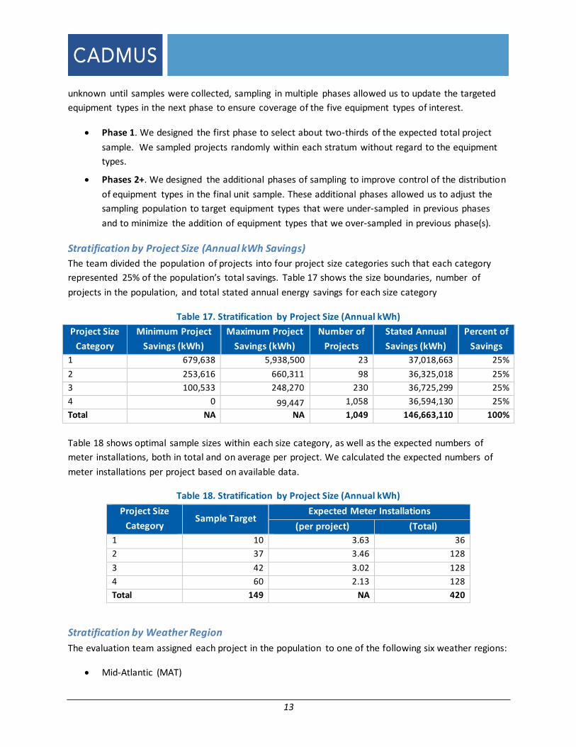
13
unknown until samples were collected, sampling in multiple phases allowed us to update the targeted
equipment types in the next phase to ensure coverage of the five equipment types of interest.
Phase 1. We designed the first phase to select about two-thirds of the expected total project
sample. We sampled projects randomly within each stratum without regard to the equipment
types.
Phases 2+. We designed the additional phases of sampling to improve control of the distribution
of equipment types in the final unit sample. These additional phases allowed us to adjust the
sampling population to target equipment types that were under-sampled in previous phases
and to minimize the addition of equipment types that we over-sampled in previous phase(s).
Stratification by Project Size (Annual kWh Savings)
The team divided the population of projects into four project size categories such that each category
represented 25% of the population’s total savings. Table 17 shows the size boundaries, number of
projects in the population, and total stated annual energy savings for each size category
Table 17. Stratification by Project Size (Annual kWh)
Project Size
Category
Minimum Project
Savings (kWh)
Maximum Project
Savings (kWh)
Number of
Projects
Stated Annual
Savings (kWh)
Percent of
Savings
1 679,638 5,938,500 23 37,018,663 25%
2 253,616 660,311 98 36,325,018 25%
3 100,533 248,270 230 36,725,299 25%
4 0 99,447 1,058 36,594,130 25%
Total NA NA 1,049 146,663,110 100%
Table 18 shows optimal sample sizes within each size category, as well as the expected numbers of
meter installations, both in total and on average per project. We calculated the expected numbers of
meter installations per project based on available data.
Table 18. Stratification by Project Size (Annual kWh)
Project Size
Category Sample Target
Expected Meter Installations
(per project) (Total)
1 10 3.63 36
2 37 3.46 128
3 42 3.02 128
4 60 2.13 128
Total 149 NA 420
Stratification by Weather Region
The evaluation team assigned each project in the population to one of the following six weather regions:
Mid-Atlantic (MAT)

14
New England – North (NEN)
New England – East (NEE)
New England – South NES)
New York – Inland (UNY)
New York – Urban/Coastal (DNY)
These weather regions match those developed for NEEP’s 2011 C&I Unitary HVAC Loadshape Project. A
“” in the table indicates the weather region(s) to which each Sponsor’s customers were assigned.
Table 19. Sponsors by Weather Region
Sponsor DNY MAT NEE NEN NES UNY
BG&E
CL&P
Con Edison
Efficiency Maine
Efficiency Vermont
First Energy
LIPA
National Grid* (NH) (MA) (RI)
NU-NSTAR
NYSERDA
Pepco
PSNH
*Since National Grid’s projects included customers in three states (NH, MA, and RI), we assigned its customers to weather regions based on the customer’s state.
Sample Size Targets
Table 20 shows the distribution of projects across project size categories and weather regions in the
population.
Table 20. Project Population Sizes
Project Size DNY MAT NEE NEN NES UNY Total
1 15 3 4 1 0 0 23
2 26 9 33 3 11 16 98
3 33 34 67 8 24 64 230
4 92 90 191 135 128 422 1,058
Total 166 136 295 147 163 502 1,409
We designed the stratified sampling sizes to balance representation by weather region, the available
sampling population, and the number of projects supported annually by each administrator. Table 21

15
shows the target sample sizes in each stratum and the total number of expected meter installations for
each project size category.
Table 21. Target Project Sample Sizes
Project Size Projects Meter
Installations DNY MAT NEE NEN NES UNY Total
1 7 1 2 0 0 0 10 36
2 10 5 11 2 4 4 36 124
3 7 7 10 3 6 9 42 126
4 6 6 10 14 10 17 63 134
Total 30 19 33 19 20 30 151 422
2.1.4 Sample Execution
The target sample sizes developed in the sample strategy represent a sample design centered around
confidence and precision goals for estimates to be summarized across projects. The final goal, however,
is to produce loadshape estimates at the unit level and summarize across unit-level estimates within
each equipment types. The evaluation team could not design the sample around this goal due to lack of
information on the distribution of units across the population.
To obtain sufficient information on each equipment type, we collected the sample using the multi-
phase, multi-stage procedure discussed above. As stated in the original sampling memo, we expected to
adjust the target sample sizes as actual sampling progressed in order to meet the meter installation
targets for each equipment type. We sampled projects according to the target sample sizes described
above, making refinements to the sampling that occurred after the first phase.
Sample Phase 1
In the first phase, we randomly sampled 107 projects13 from the study population (Table 20) based on
the target distribution across project size and weather region strata (Table 21). We then collected
detailed project information about the equipment types included within each project from the Sponsors
for the Phase 1 Project Sample.
Table 22 shows the distribution of sample sizes achieved in the Phase 1 Project Sample. The total sample
size was 88 projects (compared to the target of 107) due to high non-response rates as well as
ineligibility, verified using the detail project information collected during the first phase. Further, several
sample projects were dropped during the site visits because the actual equipment type using the VSD
did not match the documented equipment type and therefore the project was determined to be
13 We drew an additional 53 back-up projects (50% of the target sample size) to replace any primary projects that were not available. If a primary project was unavailable, we replaced it with a back-up project, randomly selected among the available back-up projects in the same stratum as the non-response or dropout project. In the end, 43 (40%) of the 107 primary projects were dropped and replaced with back-up projects.
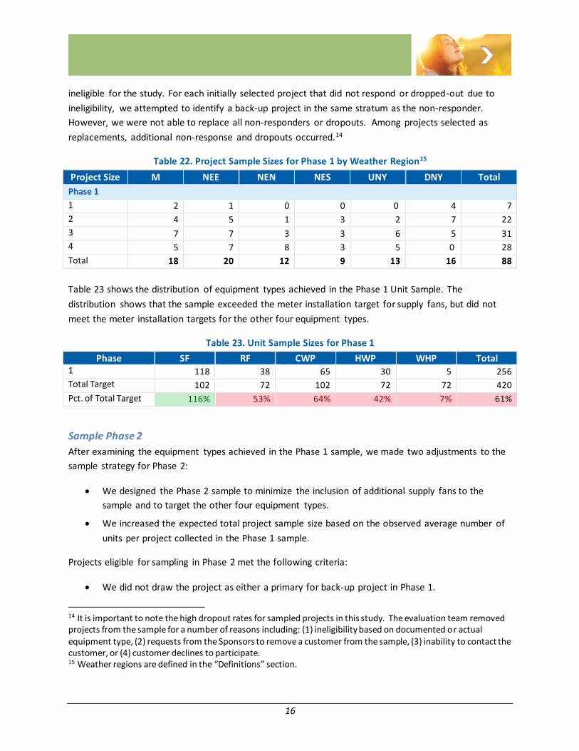
16
ineligible for the study. For each initially selected project that did not respond or dropped-out due to
ineligibility, we attempted to identify a back-up project in the same stratum as the non-responder.
However, we were not able to replace all non-responders or dropouts. Among projects selected as
replacements, additional non-response and dropouts occurred.14
Table 22. Project Sample Sizes for Phase 1 by Weather Region15
Project Size M NEE NEN NES UNY DNY Total
Phase 1
1 2 1 0 0 0 4 7
2 4 5 1 3 2 7 22
3 7 7 3 3 6 5 31
4 5 7 8 3 5 0 28
Total 18 20 12 9 13 16 88
Table 23 shows the distribution of equipment types achieved in the Phase 1 Unit Sample. The
distribution shows that the sample exceeded the meter installation target for supply fans, but did not
meet the meter installation targets for the other four equipment types.
Table 23. Unit Sample Sizes for Phase 1
Phase SF RF CWP HWP WHP Total 1 118 38 65 30 5 256
Total Target 102 72 102 72 72 420
Pct. of Total Target 116% 53% 64% 42% 7% 61%
Sample Phase 2
After examining the equipment types achieved in the Phase 1 sample, we made two adjustments to the
sample strategy for Phase 2:
We designed the Phase 2 sample to minimize the inclusion of additional supply fans to the
sample and to target the other four equipment types.
We increased the expected total project sample size based on the observed average number of
units per project collected in the Phase 1 sample.
Projects eligible for sampling in Phase 2 met the following criteria:
We did not draw the project as either a primary for back-up project in Phase 1.
14 It is important to note the high dropout rates for sampled projects in this study. The evaluation team removed projects from the sample for a number of reasons including: (1) ineligibility based on documented or actual equipment type, (2) requests from the Sponsors to remove a customer from the sample, (3) inability to contact the customer, or (4) customer declines to participate. 15 Weather regions are defined in the “Definitions” section.

17
For project with equipment type tracking data, the project included at least one VSD on one of
the following equipment types: RF, CWP, HWP, and WHP. In other words, we marked any
projects with VSDs only on supply fans as ineligible for Phase 2.
Projects with unknown equipment types were eligible to be included in the sample,
however, if a sampled project was determined to have no eligible equipment types other
than supply fans during the documentation review, recruitment phone call, or site visit, we
replaced the project with a back-up project from the same stratum when possible.
We initially sampled 45 projects during Phase 2. Table 24 shows the distribution of projects achieved in
the Phase 2 Project Sample.
Table 24. Project Sample for Phase 2
Project Size MAT NEE NEN NES UNY DNY Total PHASE 2
1 0 2 0 0 0 0 2
2 0 11 0 0 1 0 12
3 5 8 1 0 3 2 19
4 0 0 2 0 2 0 4
Total 5 21 3 0 6 2 37
Table 25 shows the distribution of equipment types included in the unit sample resulting from both
Phase 1 and Phase 2. The distribution shows that the total sample exceeded the meter installation
target for supply fans and was close to meeting the target for cooling water pumps. However, sample
sizes for RF, HWP, and WHP were still below 90% of the targeted sample sizes though, so we proceeded
to Phase 3 sampling.
Table 25. Unit Sample for Phases 1 and 2 Combined
Phase SF* RF CWP HWP WHP Total 1 118 38 65 30 5 256
2 17 20 31 15 10 93
1+2 135 58 96 45 15 349
Target 102 72 102 72 72 420
Percent of Target 132% 81% 94% 63% 21% 83%
* Although Phase 2 made ineligible any projects that had only supply fans, some projects had supply fans in addition to other
eligible equipment types. Supply fans added to the unit sample in Phase 2 are units included in these eligible, sampled Phase 2
projects.
Sample Phase 3
We performed a third phase of sampling to target the three equipment types with the smallest presence
in the population: RFs, HWP, and WSHPs. We reduced the Phase 3 population to projects that met the
following criteria:
We did not draw the project as either a primary for back-up project in Phase 1 or Phase 2.

18
For projects with equipment type tracking data, the project included at least one of the
following equipment types: RF, HWP, WHP. That is, we marked any projects that included only
SFs or CWPs as ineligible for Phase 3.
We sampled 40 projects from the Phase 3 population. Table 26 shows the distribution of projects
achieved in the Phase 3 Project Sample.
Table 26. Project Sample for Phase 3
Project Size MAT NEE NEN NES UNY DNY Total PHASE 3 1 0 0 0 0 0 0 0
2 0 1 0 0 0 0 1
3 2 9 0 1 0 1 13
4 1 13 4 9 0 0 27
Total 3 23 4 10 0 1 41
2.1.5 Final Sample for Data Collection
Table 27 shows the distribution of equipment types in the unit samples collected during each phase and
resulting overall sample sizes. The distribution shows that the sample sizes exceeded the meter
installation targets for supply fans, cooling water pumps, and hot water pumps and reached 90% of the
meter installation target for return fans.
Table 27. Phase 1+2+3 Unit Sample by Equipment Type
Phase SF RF CWP HWP WHP Total
1 118 38 65 30 5 256
2 17 20 31 15 10 93
3 2 7 22 38 3 72
Total 137 65 118 83 18 421
Target 102 72 102 72 72 420
Pct. of Target 134% 90% 116% 115% 25% 100%
The final sample includes 166 projects and 421 units across the project size and weather region strata.
Table 28 shows the distribution of projects sampled in each stratum. For each of the 166 sampled
projects, we installed power meters on up to four units (on average, we metered 2.5 units per project).
Table 28. Final Sample of Projects by Weather Region and Project Size
Project Size MAT NEE NEN NES UNY DNY Total 1 2 3 0 0 0 4 9
2 4 18 1 2 3 7 35
3 14 24 4 4 9 8 63
4 6 21 14 11 7 0 59
Total 26 66 19 17 19 19 166
Pct. of Total 16% 40% 11% 10% 11% 11% 100%

19
Table 29 shows the distribution of units by equipment type and weather region.
Table 29. Final Sample of Equipment Type by Weather Region
Equipment Type MAT NEE NEN NES UNY DNY Total Supply Fan 22 22 23 9 35 26 137 Return Fan 14 20 3 3 10 15 65 Cooling Water Pump 25 54 5 8 4 22 118 Hot Water Pump 3 46 11 12 5 6 83 WSHP Circulation Pump 1 10 4 0 3 0 18
Total 65 152 46 32 57 69 421
Pct. of Total 15% 36% 11% 8% 14% 16% 100%
Table 30 shows the distribution of units by equipment type category, weather region, and project size.

20
Table 30. Final Unit Sample by Equipment Type, Weather Region, and Project Size
Project Size MAT NEE NEN NES UNY DNY Total Supply Fans 1 0 4 0 0 0 8 12
2 8 4 1 2 4 8 27
3 6 6 6 7 17 10 52
4 8 8 16 0 14 0 46
Total 22 22 23 9 35 26 137
Return Fans 1 0 8 0 0 0 8 16
2 0 7 1 1 2 3 14
3 7 3 0 2 8 4 24
4 7 2 2 0 0 0 11
Total 14 20 3 3 10 15 65
Cooling Water Pumps 1 7 0 0 0 0 0 7
2 5 27 2 2 1 11 48
3 12 18 1 2 2 11 46
4 1 9 2 4 1 0 17
Total 25 54 5 8 4 22 118
Hot Water Pumps 1 0 0 0 0 0 0 0
2 0 8 0 0 4 2 14
3 3 21 0 0 1 4 29
4 0 17 11 12 0 0 40
Total 3 46 11 12 5 6 83
WSHP Circulation Pumps 1 0 0 0 0 0 0 0
2 0 4 0 0 0 0 4
3 1 4 4 0 2 0 11
4 0 2 0 0 1 0 3
Total 1 10 4 0 3 0 1
All Equipment Types Total 65 152 46 32 57 69 421
2.2 Sample Draw and Project Recruitment Due to the multi-phased sampling method that required the results of one sampling phase to inform the
next sampled phase, we performed the sample draw and recruitment as integrated activities. For
example, we completed for projects sampled in Phase 1 to determine the population parameters for
sampling Phase 2.
Figure 8 describes our recruitment process to engage sampled projects for this loadshape study.
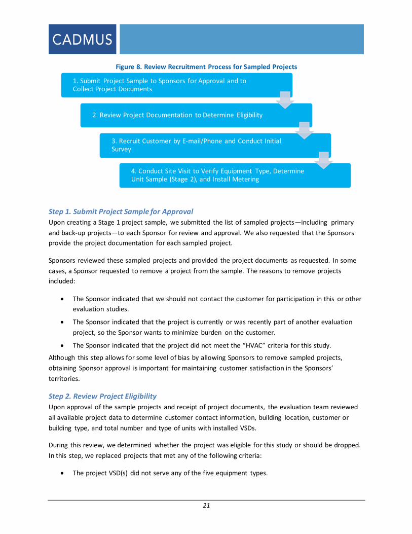
21
Figure 8. Review Recruitment Process for Sampled Projects
Step 1. Submit Project Sample for Approval
Upon creating a Stage 1 project sample, we submitted the list of sampled projects—including primary
and back-up projects—to each Sponsor for review and approval. We also requested that the Sponsors
provide the project documentation for each sampled project.
Sponsors reviewed these sampled projects and provided the project documents as requested. In some
cases, a Sponsor requested to remove a project from the sample. The reasons to remove projects
included:
The Sponsor indicated that we should not contact the customer for participation in this or other
evaluation studies.
The Sponsor indicated that the project is currently or was recently part of another evaluation
project, so the Sponsor wants to minimize burden on the customer.
The Sponsor indicated that the project did not meet the “HVAC” criteria for this study.
Although this step allows for some level of bias by allowing Sponsors to remove sampled projects,
obtaining Sponsor approval is important for maintaining customer satisfaction in the Sponsors’
territories.
Step 2. Review Project Eligibility
Upon approval of the sample projects and receipt of project documents, the evaluation team reviewed
all available project data to determine customer contact information, building location, customer or
building type, and total number and type of units with installed VSDs.
During this review, we determined whether the project was eligible for this study or should be dropped.
In this step, we replaced projects that met any of the following criteria:
The project VSD(s) did not serve any of the five equipment types.
1. Submit Project Sample to Sponsors for Approval and to Collect Project Documents
2. Review Project Documentation to Determine Eligibility
3. Recruit Customer by E-mail/Phone and Conduct Initial Survey
4. Conduct Site Visit to Verify Equipment Type, Determine Unit Sample (Stage 2), and Install Metering

22
The project VSD(s) did not serve HVAC loads.
If we could not determine the equipment type or VSD applications from the project documents, we kept
the project in the sample.
Step 3. Recruit Customer and Conduct Screening Survey
We contacted customers for recruitment and scheduling only after Sponsor approval and our review of
the project documents (Steps 1 and 2 above). For those customers with e-mail contact information, we
preceded our phone calls with a notification letter that described the purpose of the study and
requirements of participation. We then called customers to confirm details of the VSD projects, request
their participation, and schedule our initial site visit.
We dropped projects in this step for several reasons, including:
The customer declined to participate.
We determined during the phone survey that the VSD-controlled equipment did not match the
study’s target equipment types.
After four contact attempts, including e-mails and phone calls, we could not make contact with
the customer.
Step 4. Conduct Site Visit
During these site visits, we verified the documented VSD installations and completed the Stage 2
sampling to determine which units to meter. We marked sites as fully recruited only after installing our
power-metering equipment.
In some cases, we had to drop projects in this last step if we found that the installed VSD(s) did not meet
the equipment type boundaries for this study.
Replacing Dropped Projects
If we had to drop a project at any stage during the recruitment process, we replaced that project with an
approved back-up project matching the same project size stratum and weather region. If possible, we
also matched the project Sponsor in order to maintain representation of all study Sponsors.
2.3 Data Collection The team collected both primary and secondary data to support this loadshape study. Table 31
summarizes the data collection activities we completed between June 2012 and September 2013.
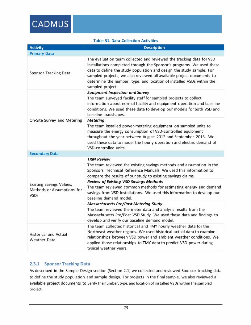
23
Table 31. Data Collection Activities
Activity Description
Primary Data
Sponsor Tracking Data
The evaluation team collected and reviewed the tracking data for VSD
installations completed through the Sponsor’s programs. We used these data to define the study population and design the study sample. For sampled projects, we also reviewed all available project documents to
determine the number, type, and location of installed VSDs within the sampled project.
On-Site Survey and Metering
Equipment Inspection and Survey
The team surveyed facility staff for sampled projects to collect information about normal facility and equipment operation and baseline
conditions. We used these data to develop our models for both VSD and baseline loadshapes.
Metering
The team installed power-metering equipment on sampled units to measure the energy consumption of VSD-controlled equipment throughout the year between August 2012 and September 2013. We
used these data to model the hourly operation and electric demand of VSD-controlled units.
Secondary Data
Existing Savings Values, Methods or Assumptions for
VSDs
TRM Review
The team reviewed the existing savings methods and assumption in the Sponsors’ Technical Reference Manuals. We used this information to
compare the results of our study to existing savings claims.
Review of Existing VSD Savings Methods The team reviewed common methods for estimating energy and demand
savings from VSD installations. We used this information to develop our baseline demand model.
Massachusetts Pre/Post Metering Study
The team reviewed the meter data and analysis results from the Massachusetts Pre/Post VSD Study. We used these data and findings to develop and verify our baseline demand model.
Historical and Actual Weather Data
The team collected historical and TMY hourly weather data for the Northeast weather regions. We used historical actual data to examine relationships between VSD power and ambient weather conditions. We
applied those relationships to TMY data to predict VSD power during typical weather years.
2.3.1 Sponsor Tracking Data
As described in the Sample Design section (Section 2.1) we collected and reviewed Sponsor tracking data
to define the study population and sample design. For projects in the final sample, we also reviewed all
available project documents to verify the number, type, and location of installed VSDs within the sampled
project.

24
2.3.2 On-Site Survey and Metering
We visited sites for sampled projects two to three times to conduct the initial survey and install data
loggers, replace the data loggers for continued monitoring (as necessary), and to remove the data
loggers.
Logger Installation: The first site visit included the majority of the on-site data collection
activity, including a survey of the building and baseline operational practices, inspection of the
project installation and verification of project data, equipment measurements and installation of
the long-term monitoring equipment, and procurement of any EMS trend data.
Interim Replacement: Some sites received an additional interim site visit for interim data
collection with the loggers left in place through August 2013 16.. These sites included motor
types with summer operation, such as cooling water pumps where the installed logger did not
have sufficient data or battery capacity to capture the extended period.
Logger Removal: The second site visit included collection of all data monitoring equipment and
a brief survey with the facility manager to review operational information, discuss whether
there were any significant changes at the facility, and answer any questions about the observed
data17 to date.
Equipment Inspection and Survey
During the first site visits, we surveyed the available facility staff member(s) to collect information to
characterize typical building and HVAC system operation for both the existing (with VSD) and pre-retrofit
(baseline) conditions. We created an iPad-based data collection form to guide these interviews and
compile all data for quality control reviews.
In some cases, the ideal site contact was either not available or not knowledgeable enough to answer all
survey questions. When possible, our field engineers collected additional contact information to follow
up on remaining questions after completing the site visit.
16 The Sponsors may opt to extend the data collection period for installations that have a strong weather dependence in order to capture additional cooled season data and equipment operation during the hottest hours of the year. With this option, data loggers will be downloaded at the end of the regular logging period (February 2013) and left through July 2013. 17 For sites with the cellular enabled (U30) data logger, analysts will review the power data before the loggers are collected and may have questions about abnormalities in the data or any observed changes in operational patterns. For all sites, we may have more specific questions about why the equipment is operated a certain way (e.g., constant speed). We want to understand why so many VSD installations are completed this way, but will ask at the end of data collection so these discussions will not influence changes in operation for the data collection period.

25
Building Information
We started each on-site survey with a series of questions about typical annual building operations. We
designed these questions to support our modeling of annual operations and to provide explanatory
information for any unexpected data. Our questions probed the following building characteristics:
Building type (using the standard list Table 32);
Seasonal building operating calendar, including observed holidays and typical shut-down
periods;
Typical daily and weekend occupancy schedules;
Description of HVAC systems;
Seasonal operating calendar for HVAC systems, including whether systems operate all year or
when the facility brings systems on/offline; and
Typical daily and weekly HVAC system operating schedules.
Table 32 shows the standard list categories we used to assign each building type.
Table 32. Building Types
Building Types
Office K-12
Restaurant Warehouse
College/University (Nonresidential) Grocery
Industrial/Manufacturing Multifamily/Dormitory
Retail Hotel/Motel/Lodging
Hospital Other
Unit Operation with VSDs
After completing our question about the general building and HVAC system, we focused on information
about the sampled VSD units. For each unit, we asked a series of questions to examine the unit’s
purpose, control settings, and typical annual operation.
Unit Operating in the Pre-Retrofit Condition
For each sampled unit, we also asked questions about how the customer operated the equipment
before installed the new VSDs.
We used the survey responses, our review of the Sponsor tracking data, and our on-site inspection to
classify the pre- and post-retrofit systems into one of the categories in Table 33. In some cases, we
documented pre-retrofit systems that were not included in the listed operational strategies (e.g.,
constant volume supply/return fan VSD control based on ambient temperature).
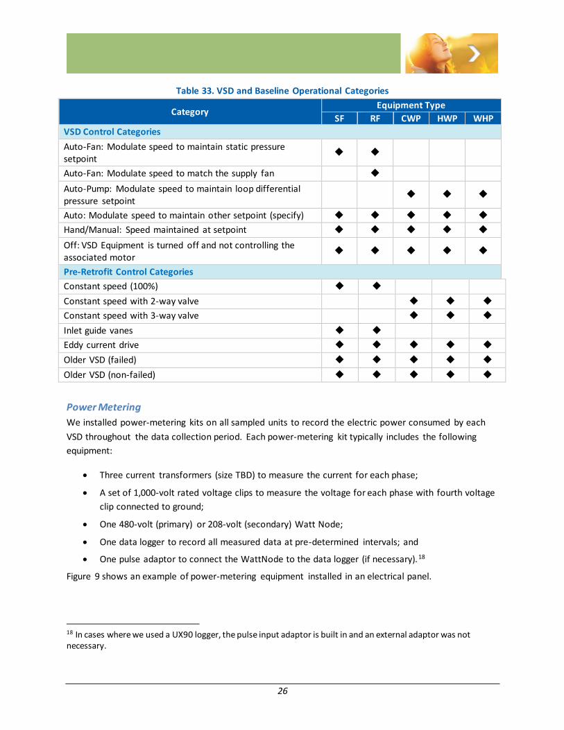
26
Table 33. VSD and Baseline Operational Categories
Category Equipment Type
SF RF CWP HWP WHP
VSD Control Categories
Auto-Fan: Modulate speed to maintain static pressure setpoint
Auto-Fan: Modulate speed to match the supply fan
Auto-Pump: Modulate speed to maintain loop differential pressure setpoint
Auto: Modulate speed to maintain other setpoint (specify)
Hand/Manual: Speed maintained at setpoint
Off: VSD Equipment is turned off and not controlling the associated motor
Pre-Retrofit Control Categories
Constant speed (100%)
Constant speed with 2-way valve
Constant speed with 3-way valve
Inlet guide vanes
Eddy current drive
Older VSD (failed)
Older VSD (non-failed)
Power Metering
We installed power-metering kits on all sampled units to record the electric power consumed by each
VSD throughout the data collection period. Each power-metering kit typically includes the following
equipment:
Three current transformers (size TBD) to measure the current for each phase;
A set of 1,000-volt rated voltage clips to measure the voltage for each phase with fourth voltage
clip connected to ground;
One 480-volt (primary) or 208-volt (secondary) Watt Node;
One data logger to record all measured data at pre-determined intervals; and
One pulse adaptor to connect the WattNode to the data logger (if necessary).18
Figure 9 shows an example of power-metering equipment installed in an electrical panel.
18 In cases where we used a UX90 logger, the pulse input adaptor is built in and an external adaptor was not necessary.

27
Figure 9. Example of Installed Power-Metering Kit
The image on the left shows the three current transducers (CTs) measuring current through the wires
for each phase of the motor. These CTs are connected to the WattNode shown in the image on the
right. The WattNode is also connected to three voltage clips that measure the voltage of each phased of
the motor. The WattNode collects and send these current and voltage data to a data logger that records
the measures values at specified intervals.
The team used the four different types of data loggers listed in Table 34.
Table 34. Power Logging Equipment
Parameter Logging Equipment Logging Frequency
kW HOBO Energy Logger (H22-001) 5-min average
kW HOBO Micro Station Data Logger (H21-002) 5-min average
kW HOBO U30 Cellular Data Logger (U30-GSM) 5-min average
kW HOBO UX90 State Logger (UX90-001) 5-min average
All set-ups include power factor measurement and satisfy the ISO New England measurement and
verification requirements.
2.3.3 Existing Values, Methods, and Assumptions for VSDs
The evaluation team reviewed multiple sources of existing savings values, methods, and assumptions for
VSD installations. These sources included the technical reference manuals used by study Sponsors or
voltage clips
Current transducers (CTs)
WattNode
HOBO UX90 State Logger with
Integrated pulse adaptor wires to CTs
wires to WattNode

28
other program administrators, other existing VSD savings models or evaluation protocols, and the
results from previous VSD evaluations.
Massachusetts Pre/Post Metering Study
Of particular interest among secondary data sources was the Massachusetts Pre/Post VSD Study. For
this study, DMI—a partner in the NEEP Loadshape study—performed up to six months of pre-retrofit
and post-retrofit metering for 22 VSD retrofit installations in Massachusetts. Cadmus, DMI, and the
NEEP Technical Committee discussed key findings from this study to shape and verify our approach for
estimating pre-retrofit power.
2.3.4 Weather Data
The evaluation team collected historical and TMY hourly weather data for the Northeast weather
regions. We matched the six weather regions used in NEEP’s 2011 C&I Unitary HVAC Loadshape Project
Final Report. We used historical actual to examine relationships between VSD power and ambient
weather conditions. We applied those relationships to TMY3 weather data to predict VSD power during
typical weather years.
2.4 Data Analysis The evaluation team used primary and secondary data to develop estimates of the savings loadshapes
and savings metrics for each sampled unit. We used these data to develop models that estimate hourly
operation and power for both the pre- and post-retrofit conditions. We then applied these hourly
models to typical weather and calendar years to estimate demand and savings loadshapes for each unit.
Figure 10 demonstrates our process to develop these unit-level savings results.

29
Figure 10. Process for Estimating Unit-Level Savings Loadshapes and Metrics
As the figure indicates, we first performed a preliminary analysis to conduct a quality inspection of the
metered and survey data. We then created the following models for each unit:
1. The hourly operating schedule indicates the percentage of time in each hour that unit is
expected to operate in a typical year. The evaluation team developed the operating schedules
based on observed post-retrofit operating patterns during the data collection periods.
2. The hourly VSD power model estimates the electric demand required by the unit when on and
operating with the connected VSD. The evaluation team used the metered on survey data to
develop hourly VSD power models for each unit.
3. The hourly baseline power model estimates the electric demand that the unit would have
required when operating in the pre-retrofit condition. In addition to the primary data, we used
secondary data to guide and verify our approach for estimating pre-retrofit operating power.
The evaluation team used secondary data to create a baseline modeling approach and
combined this approach with metered and survey data to develop hourly baseline power
models for each unit.
We used these unit-level schedules and operating power models to calculate the baseline demand
loadshape, the VSD demand loadshape, savings loadshape, and savings metrics for each unit in a typical
year.
Primary Data
Step 2. Hourly Operating Schedule
Step 4. Hourly Baseline Power Model
Step 3. Hourly VSD Power Model
Baseline Demand
Loadshape
VSD
Demand
Loadshape
Savings
Loadshape Savings Metrics
Secondary Data
Step 1. Inspect and QC

30
The following sections outline the methods for each step in our data analysis.
2.4.1 Inspect and Perform Quality Control of Primary Data
During the initial download and inspection of meter data, we performed both a quality check and a
preliminary analysis of the meter and survey data. In this review, we observed general trends in the
data, such as seasonal operation, regularity of operating schedules, maximum observed power, and
magnitude of power variations.
Data Download and Quality Control
As we retrieved data loggers, we downloaded and compiled the raw meter data.19 During this process,
the evaluation team removed loggers with data errors (as noted by field technicians) and flagged loggers
that indicated no unit operation. Next, we removed any data recorded before or on the date of
installation, after or on the date of removal, and during the date of the interim visit (if applicable). We
used the remaining data to develop hourly average status and power datasets for the period from
September 1, 2012, through August 31, 2013.
Preliminary Analysis
We created time series and “power map” figures for each unit to conduct visual inspections of the
meter data. The time series chart shows the average hourly power during the data collection period.
The power map is similar to a topographical map and illustrates variation in power demand across hours
in the day (y-axis) and days (x-axis) during the data collection period.
19 Due to the long metered periods (exceeding 12 months in some cases), we had multiple data files for each unit. We compiled these multiple data files into a single dataset that included all data for the complete data collection period.

31
Figure 11. Example of Preliminary Data Review
We used these data graphics to complete the following steps in our quality control reviews and
preliminary analysis:
Identified any gaps or anomalous data and removed from the dataset (if appropriate).
We define “gaps” in the data as any periods between the installation and removal dates
during which no data were recorded (e.g., the period between a logger stoppage and logger
replacement).20
We defined “anomalous” data as any data that do not represent the normal operation of
the unit (e.g., equipment not operating during period of interrupted electric service after
Hurricane Sandy).
We determined that it is appropriate to remove data when we can confirm that the data
does not represent normal unit operation for that period in a typical year.
Identified any changes in system operation during the data collection period, and use these to
define operating season(s). Compare these data observations to operating information collected
from on-site surveys.
20 A logger stoppage may be due to movement of the logging equipment by site personnel, logger reaching its memory capacity, or a failed battery.

32
We defined an operating season as a period during which the unit exhibits a regular
operating pattern. For example, a supply fan at a school may exhibit one pattern from
September through May (when school is in session) and a different pattern from June
through August (when the school is closed). These periods indicate distinct operating
seasons.
Operating information collected during the on-site surveys includes anecdotal information
provided by the site staff about seasonal equipment-control strategies.
2.4.2 Hourly Operating Schedule
The hourly operating schedule indicates the percentage of time in each hour of the year that we expect
the unit to operate. For example, a supply fan may operate continuously (8,760 hours per year) or on a
fixed schedule (e.g., weekdays from 6:00 a.m. to 6:00 p.m.). The sum of all hours that the unit is
operating in the unit’s operating schedule indicates the expected annual operating hours.
Post-Retrofit (VSD) Operating Schedule
We used our meter and survey data to develop the post-retrofit operating schedule for each unit. In this
process, we considered the following operating characteristics:
Operating season(s). The operating season(s) defines the date range during which we expect
the unit to operate in a typical year. For example, a fan in a commercial building will typically
have an operating season that includes the entire calendar year. However, a fan in a school may
operate only from September through May. We used both meter data and results of our on-site
interviews to determine the operating season(s) for each unit. We indicated multiple operating
seasons if meter data indicate multiple distinct operating patterns.
Operating pattern(s). The operating pattern describes the expected hourly operation within the
defined operating seasons. We categorize each unit into one of these three patterns:
Continuous operation indicates that the unit operated continuously within its operating
season.
Scheduled operation indicates that the unit operated on a regular schedule (e.g., on
weekdays from 6:00 a.m. to 6:00 p.m.) within its operating season.
Irregular operation indicates that the unit demonstrated no regular operating patterns. This
irregularity is typically due to the role of the unit as back-up or lead-lag equipment.
Rotating units. Rotating units operate in a team of similar units to serve the same load. Facility
operators rotate units to lengthen the lifetime of equipment and to provide redundancy in case
of failure. Since rotating units take turns serving the designated load, each unit operates for
only a fraction of the team’s overall schedule.
These different operating characteristics all contribute to the unit’s typical annual schedule. Figure 12
demonstrates the variety of operating schedules we observed. Each chart shows the operating status—
on or off—throughout the data collection period.

33
Figure 12. Example of Unit Operating Schedule
A
B
C
D
Unit A operated continuously throughout the 10-month data collection period. We modeled this unit’s
schedule to operate continuously throughout the year. Although the data indicate a short period of
inactivity at the beginning of June, we confirmed that this was a maintenance period that does not
represent normal operation.
Unit B operates continuously only during the heating season. We modeled this unit’s schedule to
operate continuously during the heating season and remain off otherwise. In general, we defined the
range of dates for heating, cooling, and other operating seasons by the dates indicated in the metered
and survey data.
Unit C operates on a regular schedule and only during the cooling season. We modeled this unit’s
schedule to operate according to the observed average weekly schedule during the cooling season and
to remain off outside of the cooling season.
Unit D is a rotating unit that operates with one other unit to serve a continuous and year-round load.
We modeled this unit’s schedule to operate only 50% of the time throughout the year.
Pre-Retrofit (Baseline) Operating Schedule
In this study, we assume that the pre-retrofit (baseline) operating schedule is the same as the observed
post-retrofit (VSD) operating schedule. This assumption implies that the implementation of a VSD has no
effect on the equipment operating hours, so that total operating hours are equivalent with or without a
VSD. Although a VSD could influence both the operating power and the operating hours of the
connected equipment, we determined that this study would focus only on the savings achieved by
power reductions during post-retrofit operating hours.

34
Through discussions with the NEEP Technical Committee and the EM&V Forum, we agreed on this
conservative assumption for the following reasons:
Any survey data that we collected about baseline operation are anecdotal and rely on
information provided by facility site staff during logger installation/removals. Due to the timing
and post-installation focus of this study, we could not verify the baseline schedules for any
equipment.
We have baseline operating information only for a small fraction of the sampled equipment. For
the majority of the units, the facility staff did not recall or could not report information about
the baseline equipment or operation.
We could also attribute adjustments to equipment operating schedules resulting in reduced
operating hours to retro-commissioning or other energy management system upgrades.
2.4.3 Hourly VSD Power Model
The hourly VSD power model estimates the electric demand required by the unit when operating with
the connected VSD. We analyzed relationships between measured operating power and the auxiliary
variables that may influence that power. We produced a set of hourly models for each unit that predict
the unit hourly operating power during specific operating seasons, day types, hours, and weather
conditions. By combining this power model with the unit’s operating schedule, we can predict the unit’s
hourly demand for a typical weather and calendar year.
In this section, we describe our approach to develop these hourly power models and calculate the
expected hourly VSD power for a typical weather year.
Determine Modeling Approach
As previously noted, we observed a variety of operating patterns among the studied units. We noted
that some units operated at constant power throughout the data collection period or within specific
seasons, some units showed distinct power adjustments for different seasons, and some units operated
with variable power throughout the year or within a specific season. Based on these observations, we
developed three modeling approaches to predict the VSD operating power:
Constant Power Model: For units that demonstrated constant operating power during the data
collection period, this model applies the observed operating power value regardless of
temperature or any other variable.
Temperature Model: For units that demonstrated variable power correlated with temperature,
this model uses the observed hourly correlation between temperature and power to predict
operating power using typical weather data.
Average Power Model: For units that demonstrated variable power but showed no relationship
between power and outside temperature, this model applies the measured average operating
power for each combination of operating season, day type, and hour.

35
The Average Power Model is mathematically very similar to the constant power model for units that
exhibit constant operating power. The Constant Power Model and the Average Power Models would
produce very similar, if not identical, results for constant power units.
Figure 13 depicts our process for determining the modeling approach for each unit.
Figure 13. Process to Determine VSD Power Model
Constant Power Test
During the data collection phase, we observed that a large number of units operated at constant power
during periods of scheduled operation throughout the data collection period. We performed this first
test to identify the units that always operated at constant power.
We calculated the average operating power—the expected power when the unit is on—for all hours in
the data collection period and the standard deviation on that average. Units pass this constant power
test if the ratio of the standard deviation to the average power was less than 5%, indicating minimal
variation in operating power throughout the data collection period.
Figure 14 shows the raw time-series power data for a unit that passed this constant power test.
Figure 14. Sample Unit with Constant Power for All Hours
Constant Power Test
Constant Power Model
Temperature Model
Temperature Dependence Test
Average Power Model
Pass
Fail
Pass
Fail
Create hourly datasets

36
Using this method, we identified 83 of 392 units (21%) that operated at a single constant power during
hours of scheduled operation throughout the data collection period. It is worth noting that a number of
other units seemed to operate at distinct constant power for different operating seasons (e.g., one
constant power for heating season and a different constant power for cooling season), but because of
the change in power during the data collection period, those units did not pass this initial screen. (These
units would also fail the temperature screen and default to the Average Power Model. )
Identify Auxiliary Variables
Units that did not pass the constant power test have some level of variation in operating power during
the data collection period. To analyze patterns in that variation, we reviewed the key variables that may
influence changes in a unit’s operating power. Since all the equipment in this study served HVAC loads,
we expected the variables to be:
1. Season (heating vs. cooling, academic year vs. summer session, etc.);
2. Day type (weekday or weekend);
3. Time of day (occupied vs. unoccupied); and
4. Ambient weather conditions.
Although other variables—such as static pressure in supply air ducts, differential pressure in a chilled-
water loop, or CO2 levels in a conference room—are typically the driving variables for VSD control, we
limited our list of driving variables to those for which we have measured data for all buildings and for all
hours in a typical weather year. This approach allows us develop useful models to predict operation for
a normalized year. For example, we could analyze the relationship between duct static pressure and
VSD-controlled fan speeds, but we could not use that relationship to model the fan speed in for a
normal weather year or in another weather region without also knowing what the hourly duct status
pressure would be in those scenarios.
Create Hourly Datasets
We separated the meter data for each unit into hourly datasets, or unique combinations of operating
season, day type, and hour. This disaggregation of the data allowed us to separate the influences of
each of these variables both from each other and from the influences of weather (tested in the next
step). For example, we could separately model the unit’s response to temperature at noon on a
weekday and at 8:00 p.m. on a weekday. Similarly, we could separately model the temperature
response at noon on a weekday in the winter, at noon and a weekday in the summer, and at noon on a
weekend day.
We often use this hourly modeling approach in loadshape analyses to capture the important influences
of season, day type, and time on overall system demand. The next two sections describe how we apply
this hourly modeling approach to capture those important influences on VSD operating power.
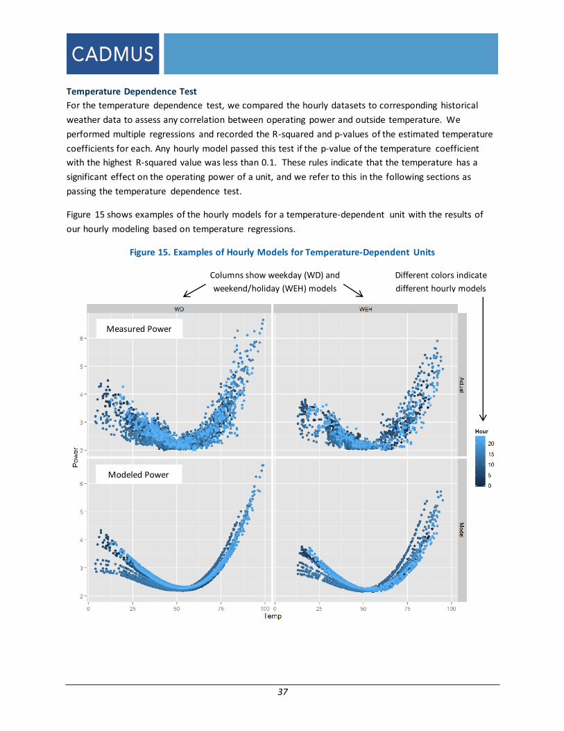
37
Temperature Dependence Test
For the temperature dependence test, we compared the hourly datasets to corresponding historical
weather data to assess any correlation between operating power and outside temperature. We
performed multiple regressions and recorded the R-squared and p-values of the estimated temperature
coefficients for each. Any hourly model passed this test if the p-value of the temperature coefficient
with the highest R-squared value was less than 0.1. These rules indicate that the temperature has a
significant effect on the operating power of a unit, and we refer to this in the following sections as
passing the temperature dependence test.
Figure 15 shows examples of the hourly models for a temperature-dependent unit with the results of
our hourly modeling based on temperature regressions.
Figure 15. Examples of Hourly Models for Temperature-Dependent Units
Measured Power
Modeled Power
Different colors indicate
different hourly models
Columns show weekday (WD) and
weekend/holiday (WEH) models

38
For hourly models that passed the temperature dependence test, we recorded the model type and
regression coefficients to define the hourly temperature model.
Average Power Model
For hourly models that failed the temperature dependence test, we assigned the average power model.
For these units, the hourly power may have varied during our data collection period, but we could not
correlate that variation with an auxiliary variable such as ambient temperature. For these units, the VSD
is likely more influenced by internal building factors—such as occupancy—than by outside weather
conditions.
It is important to note that our method of developing hourly models may results in multiple model types
for a single unit. For example, a supply fan may exhibit temperature-dependent variable power during
normal working hours but a constant power overnight and on weekends.
Estimate Hourly VSD Operating Power
For each unit, we used the set of hourly models defined in the previous steps to predict the hourly VSD
operating power for a typical weather and calendar year.
For all temperature-independent (TI) units—units for which none of the hourly models passed the
temperature dependence test—we created a single demand loadshape for the 2012 calendar year. For
all temperature-dependent (TD) units—units for which at least one hourly model indicated temperature
dependence—we created a demand loadshape for each of the six weather regions.
2.4.4 Hourly Baseline Operating Power
Because this study did not include pre-installation measurements, we used a combination of primary
and secondary data to develop a baseline model and estimate the hourly operating power for a typical
weather year.
Baseline Power Model
The baseline power model describes our approach to estimate the hourly demand of each unit in the
pre-retrofit condition. Figure 16 illustrates our baseline modeling approach and is followed by a
description for each step.

39
Figure 16. Process for Estimating Baseline Demand Loadshapes
Step 1. Identify Baseline Category
Since this study focused on VSD projects completed at least one year before our evaluation, we relied on
survey data and on-site inspections to determine the baseline category for each unit. Using the data we
collected during the site visits, we assigned each unit to one of the following baseline categories:
Constant volume (CV): A constant-volume system provides a constant volume of air or water
when operating. CV systems may include distribution equipment that varies the volume of air or
water that is supplied to the conditioned spaces or downstream HVAC equipment, but they still
provide a constant volume at the primary piece of equipment.
Variable volume not including VSD (VV): A variable-volume system modulates the flow in
response to downstream indicators (e.g., duct static pressure for a supply fan or loop differential
pressure for a distribution pump in a hydronic heating/cooling system).
Variable Speed Drive (VSD): VSDs are a subset of the VV category, enabling variable flow by
controlling the speed of the connected motor. We flagged all units for which the site contact
reported that the new VSDs replaced existing VSDs. In these cases, the customers used program
incentives to replace the old VSDs. Since VSD baselines are ineligible in all Sponsor programs, we
did not include VSD baselines in the final analysis.
Unknown: If the site contact could not describe how the pre-retrofit equipment was controlled
and the field technician could not determine the pre-retrofit system through inspection, we
recorded the baseline type as “unknown.”
For units in the VSD or unknown baseline categories, we assigned a “CV” or “VV” baseline type using the
distribution of known baselines within that equipment type. Table 35 shows the initial and adjusted
distributions of baseline categories for each equipment type.
Step 3. Determine full
speed power
Step 1. Identify baseline
category
Use performance curves
to model baseline %Power
Step 4. Calculate
Baseline Power (kW)
Assume constant full
speed power Constant Volume (CV)
Variable Volume (VV)
Variable Speed Drive (VSD) Reassign baseline category
to CV or VV based on
observed distribution for
equipment group. Unknown
Step 2. Define baseline
performance curve

40
Table 35. Reported Baseline (Pre-Retrofit) Category
Baseline Category SF RF CWP HWP WHP All
sample n = 131 n = 60 n = 109 n = 77 n = 15 n = 392
Initial Distribution Constant volume 31% 42% 35% 25% 40% 33%
Variable volume 1% 6% 0% 0% 0% 2%
Variable speed drive 1% 2% 0% 0% 0% 1%
Unknown* 66% 50% 65% 75% 60% 65%
Adjusted Distribution** Constant volume 97% 92% 100% 100% 100% 98%
Variable volume 3% 8% 0% 0% 0% 2%
* The high percentage of units with unknown baselines is due to the elapsed time (minimum of one year) since the site installed the VSDs. ** We reassigned all equipment with VSD or unknown baselines using the observed distribution of CV and VV baselines within the same equipment type category.
The high percentage of units assigned to the CV category is consistent with our expectations and observations for HVAC systems in existing buildings.
Step 2. Define Baseline Performance Curve
The baseline category determines the baseline performance curve. Table 36 shows the loadshape
approach for the two baseline system types and expected percentage of units for each baseline system
type.
Table 36. Baseline Model Approach on Baseline System Type
Baseline Category Expected Power
Performance Approach for Estimating the Baseline Performance Curve
Constant Volume (CV) Constant kW Assume that the baseline equipment will operate at constant
power (100% FLP) during all operating hours.
Variable Volume (VV) Variable kW
Assume that the baseline equipment operates at same flow rate
as measured post-retrofit equipment. Use DOE.2 eQUEST
performance curves to estimate hourly baseline %FLP based on
observed hourly post-retrofit %FLP.
Constant Volume (CV) Baseline
For baseline CV systems, which provide a constant volume of air or water through the distribution
network, we assumed that the baseline equipment operates at 100% of full load power. The pre-retrofit
metering from the Massachusetts Pre/Post VSD Study supports this assumption. In that study, the pre-
retrofit metering showed that the pre-retrofit operating power was constant for all studied units.

41
Variable Volume (VV) Baseline
For VV systems, we developed the baseline loadshape using the observed performance of the VSD
system and system performance curves from the DOE eQUEST building energy simulation tool shown in
the following figures. This approach has two built0in assumptions:
The downstream system dynamics that drive the variable flow—such as the operation of
terminal box dampers—are the same in the baseline and VSD scenarios. This assumption implies that the pre- and post- retrofit equipment serve the same building loads (a standard assumption for impact evaluations), and therefore, the baseline VV equipment will provide the same flow
rates as the VSD equipment.
Unless otherwise specified by the site staff, the baseline VV system is operational. Due to the post-installation focus of this study, we could not inspect or conduct measurements of the actual baseline systems. We had to rely on interviews with the staff to determine whether the
baseline equipment was operating as designed. Based on our experience with such HVAC distribution systems in existing buildings and the fact that the facilities were investing in a system upgrade with the VSD retrofit, it is likely that a number of these VV systems were not
operational and acted more like a CV than a VV system. However, in the absence of data—either anecdotal or physical—to quantify the percentage of non-operational systems, we
defaulted to the conservative assumption that baseline VV systems operated as designed.
We model the energy performance of baseline VV systems using standard performance curves that
describe how these systems respond to variations in flow. Figure 17 shows the relationship between
power and flow for various VV fan systems, including a VSD system.
Figure 17. eQUEST Fan System Power-Flow Performance Curves
The performance curves demonstrate how the power, represented as the percentage of full load power
(%FLP), for each system type responds to different volumes of flow.

42
We use these power-flow performance curves to develop relationships between VV system power and
VSD system power for each of the fan system types.
Figure 18. Fan Systems Normalized to VFD (shown as y=x)
We used these relationships (Figure 18) to estimate the baseline %FLP given our hourly models of VSD
%FLP.
𝐸𝑠𝑡𝑖𝑚𝑎𝑡𝑒𝑑 𝐵𝑎𝑠𝑒𝑙𝑖𝑛𝑒 %𝐹𝐿𝑃ℎ = 𝑀𝑒𝑎𝑠𝑢𝑟𝑒𝑑 𝑉𝑆𝐷 %𝐹𝐿𝑃ℎ ×𝑀𝑜𝑑𝑒𝑙 𝑉𝑉 %𝐹𝐿𝑃
𝑀𝑜𝑑𝑒𝑙 𝑉𝑆𝐷 %𝐹𝐿𝑃
Step 3. Determine Full Speed Power
We define the full load power (FLP) as the power demand when the motor is operating at full volume in
the baseline case without a VSD. We used the relationship between rated horsepower and measured
average pre-retrofit power from the Massachusetts Pre/Post Study to estimate the FLP for each unit in
this study. Figure 19 shows these data from the Massachusetts Pre/Post VSD Study.

43
Figure 19. Average Pre-Installation Power from Massachusetts Pre/Post Study Metering
The data are based on pre-installation power metering of 23 units ranging in size from 7.5 to 75 hp. The
equipment types in this study encompassed five cooling water pumps, four heating hot water pumps, 12
supply fans, one return fan, and one water source heat pump circulation pump.
We used this relationship to estimate the pre-retrofit full load power using the verified rated
horsepower for each unit and the following formula:
𝐹𝑢𝑙𝑙 𝐿𝑜𝑎𝑑 𝑃𝑜𝑤𝑒𝑟 (𝑘𝑊) = 𝑅𝑎𝑡𝑒𝑑 𝑀𝑜𝑡𝑜𝑟 ℎ𝑝 × 0.6288 𝑘𝑊/ℎ𝑝
Step 4. Calculate Baseline Power (kW)
Finally, we used the assigned baseline model, baseline performance curve, and full speed power
estimate to calculate the hourly baseline power for a typical weather and calendar year.
As we did for the VSD power model, we used the 2012 calendar year to create a single power loadshape
for all temperature-independent units and weather region data to create region-specific hourly demand
for all temperature-dependent units.
2.4.5 Unit-Level VSD Loadshapes
We use the loadshape components—unit operating schedule, VSD operating power, and baseline
operating power—to calculate the baseline, VSD, and savings loadshapes for each unit.
Figure 20. Calculation for the Unit-Level Savings Loadshape
Baseline
Demand
Loadshape
VSD
Demand
Loadshape
Savings
Loadshape
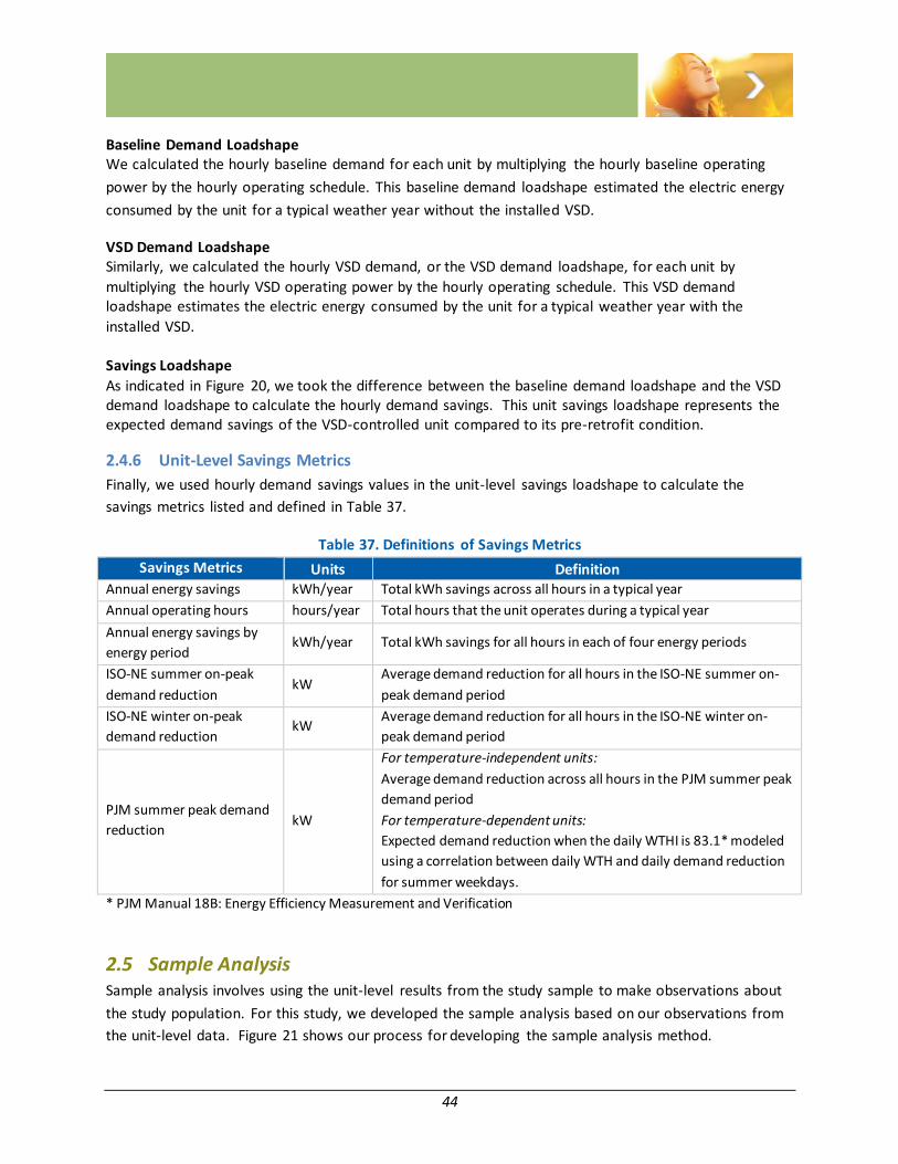
44
Baseline Demand Loadshape We calculated the hourly baseline demand for each unit by multiplying the hourly baseline operating
power by the hourly operating schedule. This baseline demand loadshape estimated the electric energy
consumed by the unit for a typical weather year without the installed VSD.
VSD Demand Loadshape Similarly, we calculated the hourly VSD demand, or the VSD demand loadshape, for each unit by
multiplying the hourly VSD operating power by the hourly operating schedule. This VSD demand loadshape estimates the electric energy consumed by the unit for a typical weather year with the
installed VSD. Savings Loadshape
As indicated in Figure 20, we took the difference between the baseline demand loadshape and the VSD demand loadshape to calculate the hourly demand savings. This unit savings loadshape represents the expected demand savings of the VSD-controlled unit compared to its pre-retrofit condition.
2.4.6 Unit-Level Savings Metrics
Finally, we used hourly demand savings values in the unit-level savings loadshape to calculate the
savings metrics listed and defined in Table 37.
Table 37. Definitions of Savings Metrics
Savings Metrics Units Definition Annual energy savings kWh/year Total kWh savings across all hours in a typical year
Annual operating hours hours/year Total hours that the unit operates during a typical year
Annual energy savings by
energy period kWh/year Total kWh savings for all hours in each of four energy periods
ISO-NE summer on-peak
demand reduction kW
Average demand reduction for all hours in the ISO-NE summer on-
peak demand period
ISO-NE winter on-peak
demand reduction kW
Average demand reduction for all hours in the ISO-NE winter on-
peak demand period
PJM summer peak demand
reduction kW
For temperature-independent units:
Average demand reduction across all hours in the PJM summer peak
demand period
For temperature-dependent units:
Expected demand reduction when the daily WTHI is 83.1* modeled
using a correlation between daily WTH and daily demand reduction
for summer weekdays.
* PJM Manual 18B: Energy Efficiency Measurement and Verification
2.5 Sample Analysis Sample analysis involves using the unit-level results from the study sample to make observations about
the study population. For this study, we developed the sample analysis based on our observations from
the unit-level data. Figure 21 shows our process for developing the sample analysis method.
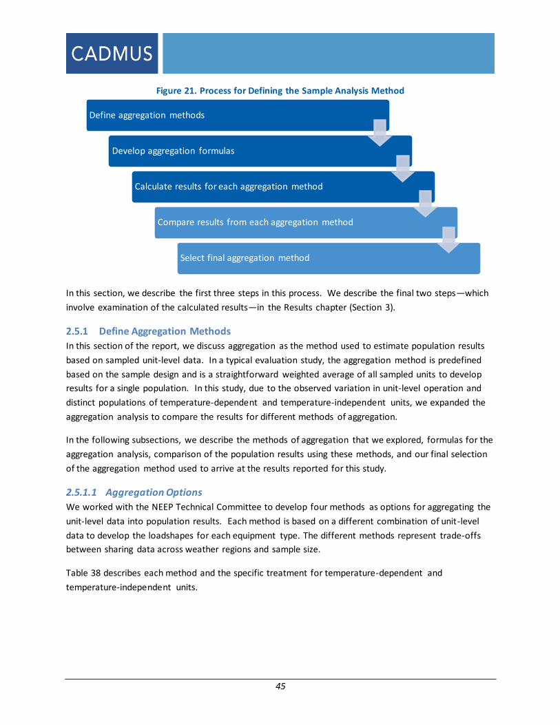
45
Figure 21. Process for Defining the Sample Analysis Method
In this section, we describe the first three steps in this process. We describe the final two steps—which
involve examination of the calculated results—in the Results chapter (Section 3).
2.5.1 Define Aggregation Methods
In this section of the report, we discuss aggregation as the method used to estimate population results
based on sampled unit-level data. In a typical evaluation study, the aggregation method is predefined
based on the sample design and is a straightforward weighted average of all sampled units to develop
results for a single population. In this study, due to the observed variation in unit-level operation and
distinct populations of temperature-dependent and temperature-independent units, we expanded the
aggregation analysis to compare the results for different methods of aggregation.
In the following subsections, we describe the methods of aggregation that we explored, formulas for the
aggregation analysis, comparison of the population results using these methods, and our final selection
of the aggregation method used to arrive at the results reported for this study.
2.5.1.1 Aggregation Options
We worked with the NEEP Technical Committee to develop four methods as options for aggregating the
unit-level data into population results. Each method is based on a different combination of unit-level
data to develop the loadshapes for each equipment type. The different methods represent trade-offs
between sharing data across weather regions and sample size.
Table 38 describes each method and the specific treatment for temperature-dependent and
temperature-independent units.
Define aggregation methods
Develop aggregation formulas
Calculate results for each aggregation method
Compare results from each aggregation method
Select final aggregation method

46
Table 38. Aggregation Methods for Population Results
Method Description Temperature-Dependent
(TD) Units
Temperature Independent
(TI) Units
A
Create loadshapes for each weather
region using only units located in
that region.
Include only units from the
weather region of interest
Unit savings modeled based
on unit weather region
Include only units from the
weather region of interest
Unit savings modeled based
on unit weather region*
B
Create loadshapes for each weather
region using all temperature-
independent units (regardless of
region) but only temperature-
dependent units that are located in
that region.
Include only units from the
weather region of interest
Unit savings modeled based
on unit weather region
Include units from all weather
regions
Unit savings modeled based
on unit weather region*
C
Create loadshapes for each weather
region using all units from all
regions. (For temperature-
dependent units outside of the
loadshape region, model the unit
loadshape using the in-region typical
weather).
Include units from all weather
regions
Unit savings modeled based
on weather region of interest
regardless of unit region
Include units from all weather
regions
Unit savings modeled based
on unit weather region*
D
Create a single combined loadshape
for the northeast using all units. For
temperature-dependent units, each
unit is modeled using typical
weather from the region in which
that unit is located.
Include units from all weather
regions
Unit savings modeled based
on unit weather region
Include units from all weather
regions
Unit savings modeled based
on unit weather region*
* For temperature-independent units, models based on unit weather region omit weather data since the
units are temperature-independent.
The first three aggregation methods (Methods A, B, and C) use the specified combinations of TI and TD
units to develop loadshapes for each of the five equipment types in each of the six weather regions.
Method A creates equipment loadshapes for each weather region using only units that are
located in that region.
Method B creates equipment loadshapes for each weather region using TD units from within the
region only, but including TI units from all regions.
Method C creates equipment loadshapes for each weather region units all units from all regions,
with the TD units modeled for the region of interest (using TMY3 weather data) regardless of
the unit’s actual location.
Method D combines all unit-level data to develop loadshapes for each equipment type across
the entire northeast region (e.g., all Sponsor territories).

47
2.5.2 Develop Aggregation Formulas
Figure 22 shows the progression of calculations to develop the population loadshapes and savings
metrics for each combination of equipment type, weather region of interest, and aggregation method.
Figure 22. Calculation Steps for Population Analysis
In Section 2.4, we described the calculation of unit-level loadshapes and savings metrics based on the
metered data and baseline model (Step 1). In Step 2, we combined the unit-level results into totals for
the TD and TI subpopulations or “domains.” In Step 3, we combined the TD and TI domain results to
develop total population results.
We provide the key formulas for these calculations below. The descriptions in Table 39 provide guidance
to interpret the formulas. Please see Appendix A for the derivation and detailed discussion of these
formulas.
Unit
Loadshapes
TI loadshapes + variance
Population Loadshapes
Unit Savings Metrics
Population Savings Metrics
TD loadshapes +
variance
TI savings metrics + variance
TD savings metrics + variance
TI and TD unit weight
factors
Step 1
Step 2
Step 3

48
Table 39. Definitions for Aggregation Formulas
Symbol Description
Y, y Population (upper-case) or unit (lower-case) demand savings
X, x Population (upper-case) or unit (lower-case) horsepower
R Population ratio estimate
R Population ratio estimate
K Domain (e.g., weather sensitive or non-weather-sensitive)
L Stratum that is defined by a unique combination of project size and weather region
I Identifier for project in the evaluation sample
J Identifier for unit in the evaluation sample
M, m Number of units in the population (upper-case) or evaluation sample (lower-case)
N, n Number of projects in the population (upper-case) or evaluation sample (lower-case)
Step 1. Calculate Unit-Level Savings Loadshapes and Metrics
In Section 2.4, we described our methods for calculating the unit-level hourly savings loadshapes and
savings metrics.
Step 2: Combine Unit-Level Results into Domain Totals
Our next step is to combine these data according to each aggregation method.
Results and Variance for TD and TI Domains
We first combine the unit-level results into totals for the TD and TI subpopulations or “domains.” We
calculate results for each domain using the following formulas:
Estimated average per-unit savings for all units in the domain:
�̅̂�𝑘 =1
�̂�𝑘
∑𝑁𝑘
𝑛𝑙
𝐿
𝑙=1
∑𝑀𝑖𝑙
𝑚𝑖𝑙
∑ 𝑦𝑖𝑗𝑙𝑘
𝑚𝑖𝑙𝑘
𝑗=1
𝑛𝑙
𝑖 =1
Estimated average per-unit horsepower for all units in the domain:
𝑋𝑘 =1
�̂�𝑘
∑𝑁𝑙
𝑛𝑙
𝐿
𝑙=1
∑𝑀𝑖𝑙
𝑚𝑖𝑙
∑ 𝑥𝑖𝑗𝑙𝑘
𝑚𝑖𝑙𝑘
𝑗=1
𝑛𝑙
𝑖 =1
Estimated variance of the total domain savings:
𝑉𝑎𝑟(𝑌𝑘 (𝑅𝑘)) = ∑ [𝑁𝑙
2
𝑛𝑙 (1 −
𝑛𝑙
𝑁𝑙
) ∑1
𝑛𝑙−1
𝑛𝑙𝑖=1
[(𝑌𝑖𝑙𝑘 − �̂�𝑘 ∙ �̂�𝑖𝑙𝑘) − (�̅�𝑙𝑘 − 𝑅𝑘 ∙ 𝑋𝑙𝑘 )]2
+𝐿𝑙=1
𝑁𝑙
𝑛𝑙 ∑
𝑀𝑖𝑙2
𝑚𝑖𝑙 (1 −
𝑚𝑖𝑙
𝑀𝑖𝑙
) ∑1
(𝑚𝑖𝑙𝑘−1)
𝑚𝑖𝑙𝑘𝑗=1
𝑛𝑙𝑖=1
[(𝑦𝑗𝑖𝑙𝑘 − 𝑅𝑘 ∙ 𝑥𝑗𝑖𝑙𝑘 ) − (�̅�𝑖𝑙𝑘 − �̂�𝑘 ∙ �̅�𝑖𝑙𝑘)]2
]

49
Population Weights for TD and TI Domains
The various combinations of TI and TD results for the aggregation methods A through D described above
require appropriate weighting of the observed occurrence of TI and TD units in each region. The
following formulas describe how we develop these regional weighting factors for the TI and TD
subpopulations.
Estimated total number of units in the domain for all regions analyzed (as defined by the
aggregation option):
�̂�𝑘 = ∑𝑁𝑙
𝑛𝑙
∑𝑀𝑖𝑙
𝑚𝑖𝑙
𝑛𝑙
𝑖 =1
𝑚𝑖𝑙𝑘
𝐿
𝑙=1
Estimated total number of units in the domain for the weather region of interest (as defined by
the aggregation option):
𝑀′̂𝑘 = ∑𝑁𝑙
𝑛𝑙
∑𝑀𝑖𝑙
𝑚𝑖𝑙
𝑛𝑙
𝑖 =1
𝑚𝑖𝑙𝑘
𝐿′
𝑙=1
Table 40 describes the comparison between the estimated number of domain units in the aggregation
(M̂k) and the estimated number of domain units in the weather region of interest (𝑀′̂𝑘 ). We use the
ratio of these two values to ensure that the total population result represents the observed ratio of TD
and TI units for each weather region.
Table 40. Domain Weighting Factors by Aggregation Method
Method Region of Interest TD Units
(k=1) TI Units
(k=2)
A Each weather region 𝑀′̂𝑘=1
�̂�𝑘=1
= 1 𝑀′̂𝑘=2
�̂�𝑘=2
= 1
B Each weather region 𝑀′̂𝑘=1
�̂�𝑘=1
= 1 𝑀′̂𝑘=2
�̂�𝑘=2
< 1
C Each weather region 𝑀′̂𝑘=1
�̂�𝑘=1
< 1 𝑀′̂𝑘=2
�̂�𝑘=2
< 1
D Northeast region combined 𝑀′̂𝑘=1
�̂�𝑘=1
= 1 𝑀′̂𝑘=2
�̂�𝑘=2
= 1

50
Step 3: Combine Domain Results into Population Totals
We then combine the TD and TI domain results to develop total population results, using the following
formulas:
Estimated total savings for all units in the complete population:
𝑌.̂ = 𝑀′̂𝑘=1 �̅̂�𝑘=1 + 𝑀′̂𝑘=2 �̂̅�𝑘=2
Estimated total horsepower of all units in the complete population:
𝑋.̂ = 𝑀′̂𝑘=1�̂�𝑘=1 + 𝑀′̂𝑘=2𝑋𝑘=2
Ratio estimate, or estimated average per-unit savings for the complete population:
𝑅.̂ =𝑌.̂
𝑋.̂=
𝑀′̂𝑘=1 �̂̅�𝑘=1 + 𝑀′̂𝑘=2 �̂̅�𝑘=2
𝑀′̂𝑘=1�̂�𝑘=1 + 𝑀′̂𝑘=2𝑋𝑘=2
Variance of the ratio estimate:
𝑉𝑎𝑟 (𝑅.) =
(𝑀′̂𝑘=1
�̂�𝑘=1
)
2
𝑉𝑎𝑟(�̂�𝑘=1(𝑅 𝑘)) + (𝑀′̂𝑘=2
�̂�𝑘=2
)
2
𝑉𝑎𝑟(�̂�𝑘=2(𝑅𝑘))
[(𝑀′̂𝑘=1
�̂�𝑘=1
) 𝑋𝑘=1 + (𝑀′̂𝑘=2
�̂�𝑘=2
) 𝑋𝑘=2]
2
2.5.3 Calculate Results for Aggregation Methods
Due to the volume of data and number of calculations, we developed code using the R programming
platform to perform the calculations. We performed quality control reviews and manual spot-checks for
each sequence of code to ensure that our program performed the calculations correctly.

51
3 Results
While the focus of this loadshape project was to develop savings loadshapes for VSDs on the selected
commercial HVAC equipment type, the analysis of collected tracking, survey, and meter data uncovered
many unexpected results. This chapter discusses the final data sample, the evaluation team’s
observations on the varied operating patterns for VSDs, and the final savings loadshapes and metrics.
3.1 Final Study Sample Table 41 shows the final sample of metered units by equipment type and weather region.
Table 41. Final Sample of Equipment Type by Weather Region
Equipment Type DNY MAT NEE NEN NES UNY Total Pct. of Total Supply Fans (SF) 35 24 21 23 20 8 131 33%
Return Fans (RF) 9 15 13 17 4 2 60 15%
Cooling Water Pumps (CWP) 4 20 22 53 3 7 109 28%
Hot Water Pumps (HWP) 5 6 3 40 11 12 77 20%
WSHP Circulation Pumps (WHP) 3 0 1 8 3 0 15 4%
Total 56 65 60 141 41 29 392 100%
Percent of Total 14% 17% 15% 36% 10% 7% 100% NA
3.1.1 Units Removed from the Dataset
We removed 29 units from the dataset for the following reasons:
Data logger not recovered from site (7)
Error in logger data or logger indicated no operation but customer did not confirm (15)
Data collection period missing critical seasons (7)
3.1.2 Units with no Operation
The meter data for 52 units indicated no operation or very low operating hours during the data
collection period. The team reviewed the survey data and contacted customers to confirm that the non-
operation indicated by the meter data was accurate for that unit. These units typically represent lag
units that only operate during periods of exceptionally high demand, or back-up units that operate only
during rare periods when primary units are unavailable.
Through discussion with the Technical Committee, the evaluation team agreed to keep these non-
operating units in the study sample.
3.2 Observations on VSD Operation The metering data showed varied operating patterns for VSD-controlled units, even within the same
equipment type and site. We used the project data and a combination of visual and analytical tests to
characterize each unit by Unit Type, Seasonality, Operating Pattern, and Operation Power.

52
Each of these characteristics affects the unit’s savings loadshape over the course of the year, influencing
both whether the unit is on or off, and the expected electric demand and savings. The variety of
characteristics across equipment types may be expected. However, the variety within each equipment
type category causes wide variations in the hourly VSD savings results.
Figure 23. Examples of Observed Variation in VSD Operation
Continuous (24/7) Operation Scheduled Operation
Co
nsta
nt
Po
wer
Var
iab
le
Pow
er
3.2.1 Motor Configuration
The motor configuration indicates the unit’s role in serving its designated HVAC load. The evaluation
team used the on-site survey and meter data results to assign each unit to one of the following
configurations:
Primary units operate as the primary, or lead, equipment to serve the designated load. When
there is a call for heating, cooling, or ventilation, the primary unit will respond to meet the load
requirements.
Lag units assist primary, or lead, equipment when the lead equipment reaches its maximum
capacity or a maximum setting. In these scenarios, the lag units will respond to serve any load
beyond what is served by the lead unit. Because the primary equipment usually serves the full
HVAC load, lag units typically operate only when the loads are unusually high.
Rotating units operate in teams of like units to serve the same load. A team of rotating units
will rotate the operating unit to serve the load while the other units “rest.” Teams are typically
two to three units and the rotation may be automated (e.g., through the facility EMS) or manual
(e.g., by facility manager). The rotation intervals vary from weekly to multiple months,
depending on the facility policy and attention of facility manager.
Back-up units rarely operate and are in place to provide redundancy for primary or rotating
units. Back-up units typically operate only when the other equipment malfunctions or is turned
off for regular maintenance activities.
Sponsor data collection forms do not collect information on the unit type, but do require that
equipment operates for a minimum of 2,000 hours per year to receive a VSD rebate.

53
3.2.2 Operating Pattern
The evaluation team reviewed metered data for each unit to characterize its operating pattern. The
operating pattern indicates when the unit is on or off during its typical operating period.
Continuous operation indicates that the unit operates during all hours in its operating season.
Continuous operation is common for HVAC equipment serving continuous loads (e.g., a 24/7
retail space).
Scheduled operation indicates that the unit operates on an hourly schedule such that the
frequency of operation varies across the hours in a day. Scheduled operation is common for
HVAC equipment serving spaces with regular occupancy schedules (e.g., office space).
Irregular operation indicates that the unit operates with no clear pattern. Irregular operation
typically indicates that the unit responds to an irregular variable or infrequent event, such as
exceptionally high loads. These exceptions may be caused by extreme weather or by unusual
activity in the conditioned space.
None indicates those units that did not operate during the data collection period, and for which
we confirmed with the customer that that logger data is accurate.
Table 42 shows the distribution of unit operating patterns within each equipment type.
Table 42. Unit Operating Pattern by Equipment Type
Operation SF RF CWP HWP WHP All
sample (n = 133) (n = 60) (n = 103) (n = 73) (n = 15) (n = 384)
Continuous 37% 25% 44% 55% 80% 42%
Scheduled* 55% 63% 42% 33% 7% 47%
Irregular 4% 5% 4% 5% 7% 4%
None 5% 7% 11% 7% 7% 7%
The data indicate that the majority of units across all equipment types operate continuously or on an
hourly schedule. Across all equipment types, only 11% either did not operate or operated irregularly.
Supply and return more frequently operated on an hourly schedule.
Cooling water pumps were equally likely to operate on a continuous or scheduled pattern.
Hot water pumps more frequently operated continuously.
Although the sample size is small for WSHP circulation pumps, 80% operate continuously.
Sponsor data collection forms do not collect information on unit operating patterns, but do require that
equipment operate for a minimum of 2,000 hours per year to receive a VSD rebate.
3.2.3 Seasonality
The team analyzed the survey data and meter data to indicate whether each unit was seasonal or non-
seasonal.
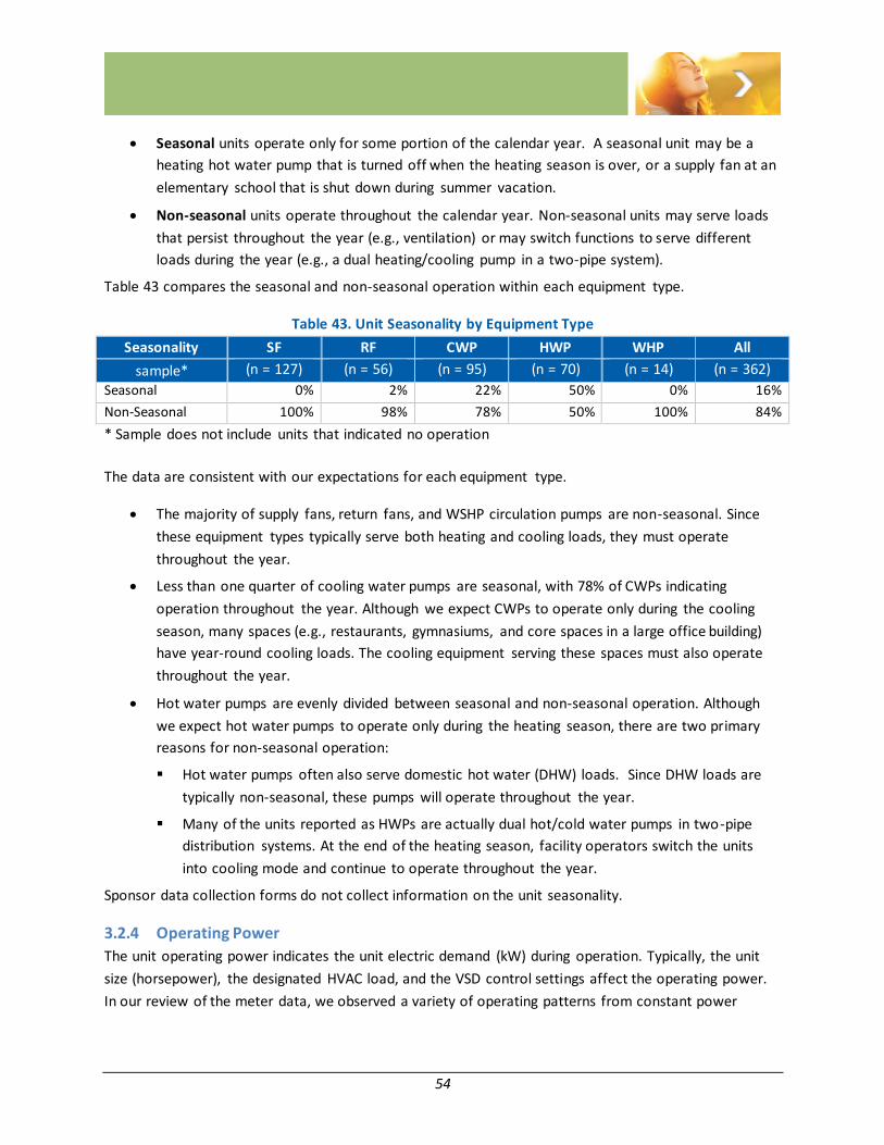
54
Seasonal units operate only for some portion of the calendar year. A seasonal unit may be a
heating hot water pump that is turned off when the heating season is over, or a supply fan at an
elementary school that is shut down during summer vacation.
Non-seasonal units operate throughout the calendar year. Non-seasonal units may serve loads
that persist throughout the year (e.g., ventilation) or may switch functions to serve different
loads during the year (e.g., a dual heating/cooling pump in a two-pipe system).
Table 43 compares the seasonal and non-seasonal operation within each equipment type.
Table 43. Unit Seasonality by Equipment Type
Seasonality SF RF CWP HWP WHP All
sample* (n = 127) (n = 56) (n = 95) (n = 70) (n = 14) (n = 362)
Seasonal 0% 2% 22% 50% 0% 16%
Non-Seasonal 100% 98% 78% 50% 100% 84%
* Sample does not include units that indicated no operation
The data are consistent with our expectations for each equipment type.
The majority of supply fans, return fans, and WSHP circulation pumps are non-seasonal. Since
these equipment types typically serve both heating and cooling loads, they must operate
throughout the year.
Less than one quarter of cooling water pumps are seasonal, with 78% of CWPs indicating
operation throughout the year. Although we expect CWPs to operate only during the cooling
season, many spaces (e.g., restaurants, gymnasiums, and core spaces in a large office building)
have year-round cooling loads. The cooling equipment serving these spaces must also operate
throughout the year.
Hot water pumps are evenly divided between seasonal and non-seasonal operation. Although
we expect hot water pumps to operate only during the heating season, there are two primary
reasons for non-seasonal operation:
Hot water pumps often also serve domestic hot water (DHW) loads. Since DHW loads are
typically non-seasonal, these pumps will operate throughout the year.
Many of the units reported as HWPs are actually dual hot/cold water pumps in two-pipe
distribution systems. At the end of the heating season, facility operators switch the units
into cooling mode and continue to operate throughout the year.
Sponsor data collection forms do not collect information on the unit seasonality.
3.2.4 Operating Power
The unit operating power indicates the unit electric demand (kW) during operation. Typically, the unit
size (horsepower), the designated HVAC load, and the VSD control settings affect the operating power.
In our review of the meter data, we observed a variety of operating patterns from constant power
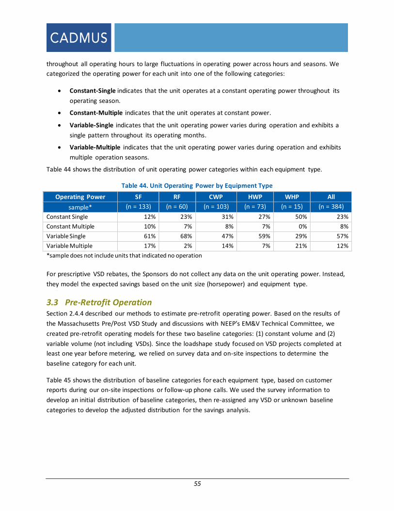
55
throughout all operating hours to large fluctuations in operating power across hours and seasons. We
categorized the operating power for each unit into one of the following categories:
Constant-Single indicates that the unit operates at a constant operating power throughout its
operating season.
Constant-Multiple indicates that the unit operates at constant power.
Variable-Single indicates that the unit operating power varies during operation and exhibits a
single pattern throughout its operating months.
Variable-Multiple indicates that the unit operating power varies during operation and exhibits
multiple operation seasons.
Table 44 shows the distribution of unit operating power categories within each equipment type.
Table 44. Unit Operating Power by Equipment Type
Operating Power SF RF CWP HWP WHP All
sample* (n = 133) (n = 60) (n = 103) (n = 73) (n = 15) (n = 384)
Constant Single 12% 23% 31% 27% 50% 23%
Constant Multiple 10% 7% 8% 7% 0% 8%
Variable Single 61% 68% 47% 59% 29% 57%
Variable Multiple 17% 2% 14% 7% 21% 12%
*sample does not include units that indicated no operation
For prescriptive VSD rebates, the Sponsors do not collect any data on the unit operating power. Instead,
they model the expected savings based on the unit size (horsepower) and equipment type.
3.3 Pre-Retrofit Operation Section 2.4.4 described our methods to estimate pre-retrofit operating power. Based on the results of
the Massachusetts Pre/Post VSD Study and discussions with NEEP’s EM&V Technical Committee, we
created pre-retrofit operating models for these two baseline categories: (1) constant volume and (2)
variable volume (not including VSDs). Since the loadshape study focused on VSD projects completed at
least one year before metering, we relied on survey data and on-site inspections to determine the
baseline category for each unit.
Table 45 shows the distribution of baseline categories for each equipment type, based on customer
reports during our on-site inspections or follow-up phone calls. We used the survey information to
develop an initial distribution of baseline categories, then re-assigned any VSD or unknown baseline
categories to develop the adjusted distribution for the savings analysis.

56
Table 45. Reported Pre-Retrofit Category
Baseline Category SF RF CWP HWP WHP All
sample n = 131 n = 60 n = 109 n = 77 n = 15 n = 392
Initial Distribution Constant volume (CV) 31% 42% 35% 25% 40% 33%
Variable volume (VV) 1% 6% 0% 0% 0% 2%
Variable speed drive* 1% 2% 0% 0% 0% 1%
Unknown** 66% 50% 65% 75% 60% 65%
Adjusted Distribution*** Constant volume 97% 92% 100% 100% 100% 98%
Variable volume 3% 8% 0% 0% 0% 2%
* Based on discussions with the NEEP Technical Committee, we reassigned VSD baselines to either CV or VV. Since VSDs are not an eligible baseline or any Sponsor programs, the team elected to remove this baseline category from the final analysis. ** The high percentage of units with unknown baselines is due to the elapsed time (minimum of one year) since the site installed the VSDs. *** We assigned all equipment with VSD or unknown baselines by randomly assigning the unit to a CV or VV baseline based on the probably of those baselines occurring in the initial, or “known” distribution.
The initial distribution shows that facility staff could not define the baseline system for almost two-
thirds of the studied units. This inability to report on the baseline conditions was prevalent for the
majority of sampled units across all equipment types. This is not surprising for a data collection effort
conducted a minimum of one year after the customer installed the VSD equipment.
Among those staff members who could recall the baseline system type and operation, the majority
indicated that the equipment operated at constant speed and power before the customer installed the
rebated VSDs. Among these, some staff indicated that although variable volume equipment existed, the
site was installing VSDs because the existing variable volume equipment was not in working condition.
We classified these cases in the constant volume category.
To estimate the adjusted distributions, the evaluation team reassigned the baseline category for units
with an unknown or VSD baseline in the initial distribution based on the observed distribution of CV and
VV baselines among the known baseline categories within each equipment group. In other words, we
randomly assigned each “unknown” or “VSD” baseline from the initial distribution to either the CV or VV
baseline category using the probability of CV or VV from the initial baselines.
The final distribution demonstrates our estimate that almost all systems operated as constant volume
prior to the VSD retrofit. Although contrary to many TRM approaches that assume a higher fraction of
variable volume baselines, we confirmed through multiple discussions with the NEEP Technical
Committee and building commissioning engineers that this high percentage of systems operating at
constant volume is consistent with field observations across existing buildings and with the pre-
installation findings from the MA VSD Pre/Post study. The following points support this finding:
57
The CV baseline category includes systems that were designed as VV but operate as CV, because
of improperly operating controls, broken equipment, etc.
The program population of buildings does not include the full C&I building stock. Rather, the
population includes only those existing buildings that participated in one of the Sponsors’ VSD
retrofit programs. Existing buildings with working variable volume systems are less likely to
participate in the programs since there is no need to replace the working VV equipment.
Eligibility requirements for several Sponsor VSD programs do not allow rebates for existing VV
systems in working condition. This filter likely further reduces the number VV baselines among
the participant population.
Our commissioning engineers agree that based on their experience in existing buildings, it is
becoming less and less common to see non-VSD VV systems in working condition. Frequently,
they will find evidence that these VV systems were part of the original design, but noted that
they are often not working. For example, we see guide vanes that are locked in place so they
effectively operate as constant volume systems.
For pumping systems, pumps without VSD controls are typically constant volume by design.
There are systems that use variable volume distribution in the building (e.g. two-way valves at
the coils), but they are typically configured using bypass valves at the plant so the primary loop
pump would still operate at full, constant volume.
Although the sample was small, the pre-retrofit metering results from the Massachusetts
Pre/Post VSD study are consistent with these assumptions. For that study, the field team
observed and metered the equipment up to a year before the VSD was installed. They identified
a couple systems that were designed as VV, but the meter data showed constant power on
those fans.
As described in Section 2.4, the evaluation team used a combination of project tracking data, meter
data, standard system curves based on the assigned baseline category, and results of the Massachusetts
Pre/Post Study data to estimate the hourly pre-retrofit demand for each unit.
3.4 Savings Results The evaluation team aggregated the unit results to calculate population average loadshapes for each
equipment type and weather region.
3.4.1 Key Assumptions
During the sampling, data collection, and analysis tasks, the evaluation team discussed methods and
findings with NEEP’s EM&V Technical Committee. This group made several key decisions to complete
the savings loadshape analysis. Although thoroughly described in Chapter 2 (Methods), we summarize
these decisions below since they affect the study results.
Pre-Retrofit Schedule. Due to the post-installation focus of the study, the evaluation team could
not monitor the pre-retrofit operating schedule. We assumed the pre-retrofit operating

58
schedule was the same as the post-retrofit operating schedule. (See Section 2.4.2 for more
details.)
Pre-Retrofit Operating Power. Due to the post-installation focus of the study, the evaluation
team could not measure pre-retrofit operating power. We modeled pre-retrofit power based on
a combination of the unit rated horsepower, metered post-installation power, and results of the
Massachusetts Pre/Post metering study. (See Section 2.4.4 for more details.)
Units with Baseline VSD. A small number of interviewed site staff said the new VSDs replaced
existing VSDs. Since replacement of existing VSDs is not eligible in the Sponsor’s programs, we
modeled these units as if they had been new VFD installations instead of replacement of existing
VFDs by assigning assigned a new baseline category for these units based on the observed
distribution of known baseline categories for units of the same equipment type.
Non-Operating Units. Our metering and on-site data collection indicated that 52 of 392 (<14%)
units have low operating hours due to rotating, lead-lag, or back-up control strategies. We
retained these units in the study sample to represent these occurrences as we observed them in
the study population (see Section 3.1 for more details).
3.4.2 Selection of Aggregation Method
The team used these aggregation formulas to calculate the population savings results and precision for
each combination of equipment type, region of interest, and aggregation method. Due to the volume of
data and number of calculations, we developed code using the R programming platform to perform the
calculations. We performed quality control reviews and manual spot-checks for each sequence of code
to ensure that our program performed the calculations correctly.
Review and Comparison of Aggregation Method Results
Once we completed the calculations for each aggregation method, we examined the results to
determine their interpretability, consistency, and overall value to NEEP members. We reviewed these
results with the NEEP Technical Committee to determine the most appropriate set of savings results for
the Sponsors. During this review, we:
Determined whether the results could be interpreted based on the characteristics of each
equipment type and expectations about savings within each geographic region;
Created summary information to review mean values and confidence intervals for each
combination of aggregation method, weather region, and equipment type to support our
discussions;
Examined the consistency between results calculated using each aggregation method within
each equipment type and across regions; and
Compared our findings to existing savings assumptions in the Sponsor’s technical reference
manuals.
In our discussions with the NEEP Technical Committee, we combined these observations with practical
considerations—such as maintaining consistency in aggregation methods across equipment types—to

59
determine the value of results to NEEP members. With the guidance of the NEEP Technical Committee,
we selected a single aggregation method for the study.
Figure 24 shows the population results for annual energy savings (kwp/hp) for supply fans as an example
displaying results using the four aggregation methods.
Figure 24. Population Results for Supply Fans by Aggregation Method (SF)
The horizontal axis represents annual energy savings (annual ΔkWh per horsepower). We present the
regional-level results as confidence intervals with points that represent estimated mean savings in the
center of the bar that spans the 90% confidence interval. The results are displayed from top to bottom
in groups according to the aggregation method. Results for Method A, which utilizes regional units only,
is displayed at the top of the plot. Methods B and C, which combine units across regions depending on
temperature dependence/independence, are next. Finally, the combined northeast (“NEEP”) estimate,
calculated using Method D, is provided at the bottom of the plot. The column on the right side of each
figure indicates the region corresponding to each confidence interval.
The plot helps us to compare results for a single equipment type. Each interval can be interpreted as
follows: we are 90% confident that the interval covers the true mean loadshape. Although we have
calculated a point estimate, we know that it is not equal to the true mean, but create the confidence
interval to give an idea of the range of values the true mean is likely to take, based on the variance of
observed values and the sampling uncertainty.
60
The bottom interval in Figure 24 shows that we are 90% confident that the interval from 1,500 to 2,500
kWh/HP covers the population mean SF loadshape for the entire NEEP region. Similarly, using Method C,
we are 90% confident that the interval ranging from 1,200 to 2,800 kWh/HP covers the UNY mean
loadshape estimated using Method C. The wider interval for UNY in Method C results from higher
variance in the unit-level observations. Each confidence interval provides us with the range of plausible
values that the true loadshape mean could take. In cases where we calculate confidence intervals for
independent samples, such as in Method A, overlapping confidence intervals indicate that a statistical
test would conclude that the means are not significantly different from one another. The estimates from
one method to the other are not independent (the same data were used to estimate the interval in
Method A UNY as in the NEEP interval), so we cannot make this strong an assertion. However, the
intervals do give an indication of the range of values that the mean loadshape could take. We compare
them and the extent of their overlap to get an idea of how similar or different the mean resulting from
each aggregation method could be.
As illustrated in Figure 24, the confidence intervals within aggregation Method A, B, and C are
overlapping, indicating that the mean loadshape values among the regions could lie in the same range.
Further, the estimates are similar across aggregation methods. The NEEP confidence interval generated
using Method D for the savings that encompasses all units from all regions covers a range that lies
within the other regional intervals but provides a narrower margin of error around the mean since all
unit-level observations were used to estimate the mean and standard error for the NEEP region. We
observe similar results for the other equipment types and metrics (kWh/HP, SPkW/HP, and WPkW/HP).
A few exceptions did occur. Most notably, the results in Figure 25 illustrate that the WHP confidence
intervals for average savings have little overlap between regions, indicating possibly significantly
different mean savings for each region. For example, the estimated mean for Upstate New York (UNY) is
notably higher than the other regions (Methods A, B, and C). However, we concluded that this result
may be difficult to interpret and should not be solely attributed to regional differences.

61
Figure 25. Population Results for WSHP Circulation Pumps by Aggregation Method (WHP)
For other equipment types and savings metrics, the confidence intervals for some regions spanned zero
but were positive for others. We did not believe in the interpretation of zero savings for a HWP in
downstate New York (DNY) or the Mid-Atlantic (MAT), for example, but positive savings in other regions
made sense based on physical characteristics of the units.
Aggregation Method Selection
As noted above, we explored multiple interpretations of the population results to determine the most
appropriate aggregation method to develop final savings results for the NEEP Sponsors. In particular, we
considered:
Consistency among results where overlapping confidence intervals indicated that average
savings loadshapes are not significantly different across regions for the majority of equipment
types and metrics;
Difficulty in attributing results to regional differences in cases where confidence intervals
suggest the savings loadshapes are significantly different from region to region;
Questionable findings in cases where confidence intervals contain zero, leading to the
conclusion that the population savings is not significantly different from zero—when this occurs
in one region but not another for the same equipment type; and
Small sample sizes at the regional level and the observed variation in performance at the unit-
level.

62
Based on our collaborative review with the NEEP Technical Committee, we concluded that aggregation
method D—providing results at the regional level—would provide the most utility to NEEP members.
3.4.3 Savings Metrics
The team used the aggregation method and formulas described in the previous section to calculate
population averages for the savings metrics defined in Section 2.4.6:
Annual energy savings per unit horsepower (kWh/hp)
Energy period savings per unit horsepower (kWh/hp)
ISO-NE summer on-peak demand savings per unit horsepower (kW/hp)
ISO-NE winter on-peak demand savings per unit horsepower (kW/hp)
PJM summer peak demand savings per unit horsepower (kW/hp)
The following tables show the population savings estimates and associated relative precision (RP) values
for each equipment type. Because the savings are based on an aggregation of all VSD units and projects
across all Sponsor states (Aggregation Method D), the results represent the expected average across all
Sponsor territories.
Table 46 shows the estimated annual energy savings per horsepower for units across the Northeast
region. We present the annual energy savings in units of kWh per hp.
Table 46. Annual Energy Savings per Unit Horsepower
Equipment Type kWh/hp RP @ 90% RP @ 80%
Supply Fans 2,033 23.5% 18.3%
Return Fans 1,788 13.8% 10.8%
Cooling Water Pumps 1,633 17.7% 13.8%
Hot Water Pumps 1,548 18.4% 14.3%
WSHP Circulation Pumps 2,562 12.8% 10.0%
* Results apply for all units across the northeast region.
Table 47 shows the estimated allocation of annual energy savings for each energy period. We present
the energy period savings in units of kWh per hp. The last column indicates that across all equipment
types, about half of the annual energy savings occur in the winter on peak period and less than 12% of
the annual energy savings occur in the summer off peak period.

63
Table 47. Energy Period Savings per Unit Horsepower
Table 48 shows the estimated demand reduction value for the ISO-NE summer on-peak period. We
present these summer demand savings in units of kW per hp.
Table 48. ISO-NE Summer On-Peak Demand Savings per Unit Horsepower
Equipment Type kW/hp RP @ 90% RP @ 80%
Supply Fans 0.288 18.8% 14.6%
Return Fans 0.302 11.9% 9.3%
Cooling Water Pumps 0.183 16.7% 13.0%
Hot Water Pumps 0.096 34.1% 26.5%
WSHP Circulation Pumps 0.229 22.0% 17.1%
* Results apply for all units across the northeast region.
Table 49 shows the estimated demand reduction value for the ISO-NE winter on-peak period. We
present these winter demand savings in units of kW per hp.
Equipment Type Energy Period kWh/hp RP @ 90% RP @ 80% % Annual Energy Savings
Summer On Peak 489 21.6% 16.8% 24%
Summer Off Peak 187 29.4% 22.9% 9%
Winter On Peak 982 21.6% 16.8% 48%
Winter Off Peak 376 29.1% 22.7% 18%
Summer On Peak 469 13.9% 10.8% 26%
Summer Off Peak 119 24.4% 19.0% 7%
Winter On Peak 959 13.4% 10.5% 54%
Winter Off Peak 241 24.4% 19.0% 13%
Summer On Peak 363 16.9% 13.1% 22%
Summer Off Peak 177 19.8% 15.4% 11%
Winter On Peak 743 17.4% 13.5% 45%
Winter Off Peak 350 19.8% 15.4% 21%
Summer On Peak 190 32.3% 25.2% 12%
Summer Off Peak 91 32.6% 25.4% 6%
Winter On Peak 850 20.5% 16.0% 55%
Winter Off Peak 418 21.5% 16.8% 27%
Summer On Peak 520 15.4% 12.0% 20%
Summer Off Peak 285 12.8% 10.0% 11%
Winter On Peak 1,166 12.4% 9.6% 46%
Winter Off Peak 590 12.1% 9.5% 23%
WSHP Circulation Pumps
Hot Water Pumps
Cooling Water Pumps
Return Fans
Supply Fans
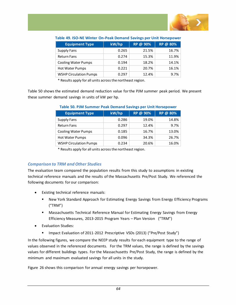
64
Table 49. ISO-NE Winter On-Peak Demand Savings per Unit Horsepower
Equipment Type kW/hp RP @ 90% RP @ 80%
Supply Fans 0.265 21.5% 16.7%
Return Fans 0.274 15.3% 11.9%
Cooling Water Pumps 0.194 18.2% 14.1%
Hot Water Pumps 0.221 20.7% 16.1%
WSHP Circulation Pumps 0.297 12.4% 9.7%
* Results apply for all units across the northeast region.
Table 50 shows the estimated demand reduction value for the PJM summer peak period. We present
these summer demand savings in units of kW per hp.
Table 50. PJM Summer Peak Demand Savings per Unit Horsepower
Equipment Type kW/hp RP @ 90% RP @ 80%
Supply Fans 0.286 19.0% 14.8%
Return Fans 0.297 12.4% 9.7%
Cooling Water Pumps 0.185 16.7% 13.0%
Hot Water Pumps 0.096 34.3% 26.7%
WSHP Circulation Pumps 0.234 20.6% 16.0%
* Results apply for all units across the northeast region.
Comparison to TRM and Other Studies
The evaluation team compared the population results from this study to assumptions in existing
technical reference manuals and the results of the Massachusetts Pre/Post Study. We referenced the
following documents for our comparison:
Existing technical reference manuals:
New York Standard Approach for Estimating Energy Savings from Energy Efficiency Programs
(“TRM”)
Massachusetts Technical Reference Manual for Estimating Energy Savings from Energy
Efficiency Measures, 2013-2015 Program Years – Plan Version (“TRM”)
Evaluation Studies:
Impact Evaluation of 2011-2012 Prescriptive VSDs (2013) (“Pre/Post Study”)
In the following figures, we compare the NEEP study results for each equipment type to the range of
values observed in the referenced documents. For the TRM values, the range is defined by the savings
values for different buildings types. For the Massachusetts Pre/Post Study, the range is defined by the
minimum and maximum evaluated savings for all units in the study.
Figure 26 shows this comparison for annual energy savings per horsepower.
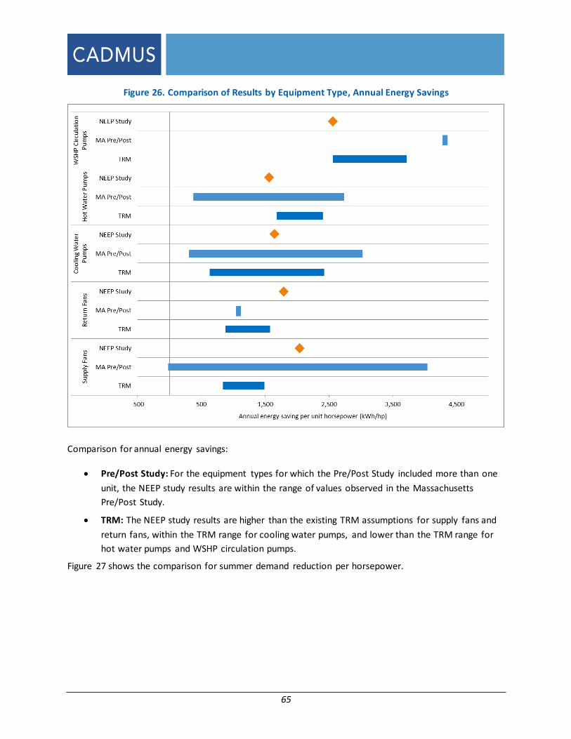
65
Figure 26. Comparison of Results by Equipment Type, Annual Energy Savings
Comparison for annual energy savings:
Pre/Post Study: For the equipment types for which the Pre/Post Study included more than one
unit, the NEEP study results are within the range of values observed in the Massachusetts
Pre/Post Study.
TRM: The NEEP study results are higher than the existing TRM assumptions for supply fans and
return fans, within the TRM range for cooling water pumps, and lower than the TRM range for
hot water pumps and WSHP circulation pumps.
Figure 27 shows the comparison for summer demand reduction per horsepower.

66
Figure 27. Comparison of Results by Equipment Type, ISO-NE Summer On-Peak Savings
Comparison for ISO-NE summer on-peak savings:
Pre/Post Study: For the equipment types for which the Pre/Post Study included more than one
unit, the NEEP study results are within the range of values observed in the Massachusetts
Pre/Post Study.
TRM: For WSHP circulation pumps, the NEEP study value is within the range of TRM
assumptions. For the other equipment types, the TRM provides a single savings value across all
building types. For hot water pumps, the NEEP savings are lower than the TRM estimate. For all
other equipment—supply fans, return fans, and cooling water pumps—the NEEP savings are
higher than the TRM estimate.
Figure 28 shows the comparison for winter demand reduction per horsepower.

67
Figure 28. Comparison of Results by Equipment Type, ISO-NE Winter On-Peak Savings
Comparison for ISO-NE winter on-peak savings:
Pre/Post Study:
For hot water pumps and supply fans, the NEEP study results are within the range of values
observed in the Massachusetts Pre/Post Study.
None of the cooling water pumps in the Pre/Post Study produce winter peak savings
because they did not operate during the winter season; however, the NEEP Study indicate
savings for a fraction of CWPs that operate year-round.
The Pre/Post Study had only one sample point for WSHP circulation pumps and return fans.
The NEEP Study average savings for WSHP are lower than observed in the Pre/Post and the
NEEP Study average savings for return fans are similar to the observed value in the Pre/Post
Study.
TRM: The NEEP study results are within the TRM range for hot water pumps and WSHP
circulation pumps. The NEEP average for cooling water pumps is lower than the TRM value. The
NEEP average for supply and return fans is higher than the TRM values.

68
3.4.4 Key Findings that Explain the Results
We uncovered multiple important findings that guided our analysis approach and dictated our
recommendation for a single set of savings results averaged across the NEEP region.
Variable speed drives frequently operate at constant speed.
Our on-site observations and metering data showed that customers operated at least one third of VSD-
controlled motors at a constant speed (typically less than full speed) during the nine- to 12-month data
collection period. Similarly, the Massachusetts Pre/Post VSD Study found that customers operated more
than two-thirds of the metered VSDs at constant speed. When we discussed this operating strategy
during our on-site interviews,21 some facility operators indicated that they intended this constant speed
operation while others indicated that they had not fully commissioned the VSD equipment. Although we
expect VSDs to vary the motor speed depending on load conditions, the observed constant speed
operation may result in higher energy savings during peak demand periods compared to when standard
savings assumptions that VSD-controlled motors operate at or close to full speed during peak
conditions.
Operators may select constant speed operation over variable speed operation.
Although we expect operators to use new variable speed drives to vary the operating speed of the
motor, we found that it is not uncommon for operators to choose to operate the motor at a constant
speed setting. Through discussions with facility staff in this study and our building commissioning
engineers, we identified several reasons an operator may choose to use a VSD to operate a motor at
constant speed:
Operators may use a VSD to dial in on a reduced constant flow requirements. Reduced constant
flow could also be achieved by using a valve or damper to throttle the flow or for certain
pumping applications modifications could be made to the pump impellers. Compared to the
throttling option, the VSD substantially reduces power requirements, energy consumption, and
energy costs. Compared to the impeller modification option, the VSD allows the operator to
keep the existing equipment in place and retains the flexibility of increasing speed (and capacity)
if needed in the future.
Operators may forgo the cost of implementing the controls for variable speed operation and
instead settle on a reduced constant speed that is acceptable. Implementing controls may
require installing new flow or pressure sensors, connecting those sensors and the VSD to a
central EMS, programming controls sequences, and commissioning the system to ensure that
the controls work correctly. Due to the cost and time requirements, operators may prefer to
operate the equipment at a constant speed that meets the generally meets flow
requirements. This constant speed may be higher than the necessary for periods of low load,
but still reduces energy consumption and costs compared to constant speed. The installation of
21 We asked these questions during removals at the end of our data collection period to minimize any influence on the facility’s typical operation.

69
the VSD allows them to take advantage of further operational modifications if the controls are
updated in the future.
Variable speed drive performance often does not track outside temperature.
In addition to a large percentage of VSDs that operated at a constant speed setting (discussed above),
our unit-level data analysis demonstrated that the operating power for more than half of the units did
not correlate with ambient temperature. Unlike larger equipment that operates to meet whole-building
HVAC loads, internal variables such as occupancy or occupant activity may be more influential to VSD
performance than external variables such as ambient temperature.
The savings estimates for each weather region are similar and similarly diverse.
In our aggregation analysis, we calculated average savings for each weather region and compared
savings estimates between regions as well as to the average across all regions combined (NEEP region).
The comparison showed that the confidence intervals for the regions overlap in most cases, suggesting
that the average results are not very different from region to region. The confidence interval for the
combined NEEP region covered a range that lies within the other regional intervals but provided a
narrower margin of error around the mean. Further, we found that the variation in operation was
similar from region to region, which provided another indication that regional differences were small.
Due to these findings, we present average savings across all six weather regions.
Most pre-retrofit equipment operates at constant power.
The evaluation team’s on-site survey and secondary data review indicated that a majority of pre-retrofit
equipment operated at constant power. As indicated in Table 5, we modeled 98% of the pre-retrofit
systems at constant power (after removing several occurrences of VSD baselines from the sample).
Although standard VSD assumptions often model other variable flow systems as the baseline for VSD
retrofit project, our research suggests that even when these variable flow systems exist they are not in
working condition. Our research is supported by the Massachusetts Pre/Post VSD Study, which
demonstrated constant power operation for 100% of the pre-retrofit systems.
3.4.5 Application of Results
Implementers in the Northeast and Mid-Atlantic states may use these results to estimate the savings for
VSD installations that meet the following characteristics:
The VSD is retrofitted on HVAC equipment in an existing nonresidential building and does not
replace an existing, working VSD.
The VSD controls a motor no larger than 200 horsepower.
The VSD controls a motor driving one of these equipment types: (1) supply fans, (2) return fans,
(3) chilled water plant distribution pumps, (4) hot water distribution pumps, and (5) water
source heat pump distribution pumps.
The controlled equipment serves an HVAC load.

70
When using these results, the implementer should calculate the desired savings parameter by
multiplying the rated horsepower of the motor or total horsepower of the population of motors by the
appropriate savings factor from the tables above. For example, to estimate the annual energy savings
for a VSD retrofit project on a 50-hp supply fan, the implementer should multiply 50 (the rated
horsepower of the existing motor) by the appropriate savings factor from Table 6. Similarly, the Sponsor
may estimate the ISO-NE on-peak demand reduction by multiplying 50 (the rated horsepower) by the
appropriate demand savings factor from Table 7.
Dissimilar to many TRM savings approaches that provide savings factors by building type or that use
engineering algorithms to estimate savings using project-specific input parameters, the results of this
study are averaged savings that account for the varied performance of VSD installations across building
types and weather regions in the Northeast and mid-Atlantic states. This study does not deny the
influence of building operating hours or ambient temperature on VSD performance; however, the
diversity of equipment performance demonstrated in this study indicates that these two variables are
not reliable predictors for VSD performance. As discussed in this report, many other factors such as
equipment operating schedules, motor configuration, and VSD control strategy also influence VSD
performance and savings estimates.
These study results are based on direct and long-term measurements of nearly 400 VSD installations and
account for the diversity of motor sizes, building types, HVAC loads, and operating strategies, and
seasonal differences across the northeast. The results also account for recent, measured findings about
pre-retrofit performance.

71
4 Recommendations
The evaluation team offers the following recommendations for implementers and evaluators of VSD
projects to improve the energy savings of VSD installations and the effectiveness of VSD programs.
Recommendations for Implementers
Continue to promote the installation of VSD on existing equipment.
VSD retrofit projects are achieving significant energy and demand savings across the
Northeast and Mid-Atlantic regions.
To ensure that VSDs operate as intended to achieve energy and demand savings, Program
Administrators should integrate VSD control and commissioning requirements into program
implementation activities. Application forms should require specification of the intended control
strategy, and post-installation inspection should include verification of commissioned VSD
control sequences.
We observed, during the site visits and in our reviews of the metered data, that many
customers operate their VSDs at constant speed. In some cases, customers intend to
operate VSDs at constant speed, but for many customers this constant speed operation is
due to incomplete project commissioning. In addition, we found that a larger percentage of
VSDs operated at constant power in the Massachusetts Pre/Post VSD Study (conducted
immediately before and after VSD installation) compared to the NEEP Study (conducted at
least one year after installation). We assume that the lower percentage of constant speed
units observed in this study is due to the longer period of elapsed time after the VSD
installation allowing more customers to complete commissioning.
As VSDs saturate the existing building stock, the Program Administrators should take more
care in screening project eligibility.
For several sampled projects, the rebated VSD units replaced existing VSD units at the end
of their useful lives. Although we did not include those baseline occurrences in this study,
these observations are evidence of projects receiving program incentives despite
ineligibility.
To support future evaluation efforts, the Program Administrators should add pre-retrofit data
collection requirements to program application forms. At minimum, the PAs should require
customers to specify the baseline system type and working condition of that system and
operating schedule for the baseline equipment.
Information about baseline operation is limited in Sponsor tracking data and difficult to
collect after customers complete VSD projects. Since baseline operation is a critical
component for estimating energy and peak demand savings, it is important for the programs
to record the working condition of baseline systems as well as the existing operating
strategy and schedule.

72
Recommendations for Evaluators
The timing of the post-installation inspection and metering is important. Our findings suggest
the customers may take a year or longer installing the VSD to set up the controls and fully
commission the system. Performing evaluation activities within a year of installation will provide
accurate first-year results but may not accurately reflect VSD performance in the following
years.
When metering VSD power for energy analyses, the evaluator should examine seasonal
operation defined for each facility. Seasons may be associated with changes in equipment
purpose (e.g., heating or cooling), occupancy patterns (e.g., academic year vs. vacation periods),
or other parameter such as control strategy (e.g., constant vs. variable speed).
Customers use HVAC motors differently throughout the year. This is especially true for
equipment in seasonal facilities and for equipment that serve both heating and cooling
loads.