1

Valuing mortality risk reductions for policy: a meta-analytic approach

Prepared by the U.S. Environmental Protection Agency’s Office of Policy,

National Center for Environmental Economics for review by the EPA’s Science Advisory Board, Environmental Economics Advisory Committee

February 2016

1 Introduction In pursuing its mission to protect human health and the environment, the EPA issues regulations with the goal of reducing environmental risks to human health. These rules are informed by scientific analyses and often include benefit-cost analyses. Indeed, benefit-cost analyses are prepared for every economically significant regulation—those with an estimated economic impact of $100 million or more in any one year—and others as required by law.

The value of reductions in people’s mortality risks figure prominently in the estimated benefits for many regulations issued by the EPA.1 In 2004, as part of ongoing efforts to improve its regulatory impact analyses, the Agency began to explore alternative approaches for updating its mortality risk value estimates. On several occasions during this process, the EPA enlisted the expertise of its Science Advisory Board’s Environmental Economics Advisory Committee (SAB-EEAC).2 This White Paper represents the culmination of this effort and provides a description of the Agency’s proposed approach for estimating values for reductions in mortality risk for use in its benefit-cost analyses.

Intended primarily for review by the SAB-EEAC, this White Paper describes the EPA’s application and implementation of recent SAB recommendations regarding updates to the EPA’s estimate of the value of mortality risk reductions, also known as the “value of a statistical life” (VSL). The main purpose of this White Paper is to provide a detailed account and explanation of the steps that the EPA has taken to update its estimate of the VSL for use in benefit-cost analyses

1 For air rules, the reduction in expected fatalities each year accounts for over 90% of total monetized benefits from PM2.5 and ozone; for drinking water standards (cancer and microbial risks), reduced mortality risk accounts for upwards of 80% of monetized benefits. 2 See Appendix A for a brief review of EPA’s engagement with the SAB’s Environmental Economics Advisory Committee on issues related to mortality risk valuation.

2

based on the recommendations received during the SAB review conducted in 2010. The EPA is soliciting general feedback and specific comments on the application of the SAB recommendations and resulting estimation methodology with the ultimate goal of incorporating the revised approach and results into its Guidelines for Preparing Economic Analyses (USEPA 2010a). The EPA also intends to introduce new terminology to replace the often-misunderstood “value of statistical life” moniker once the estimate is updated. For the purposes of this White Paper we retain the commonly-used “VSL” nomenclature.

The remainder of this White Paper is organized as follows. Section 2 provides necessary background: a brief summary of existing EPA guidance on valuing mortality risk reductions and the most recent recommendations provided by the SAB-EEAC. Section 3 describes the selection criteria used to assemble the meta-analysis dataset that forms the basis of our updated estimate of the VSL and provides a synopsis of the studies selected when the criteria recommended by the SAB-EEAC are applied to the published literature. Section 4 provides a detailed description of the estimation approach, Section 5 presents and discusses the results, and Section 6 provides a summary and concluding thoughts.

2 Background

2.1 Existing EPA guidance

To value reductions in mortality risks in its benefit-cost analyses, the EPA uses an estimate of the VSL equal to $4.8 million ($1990). This central estimate was derived from 26 estimates of the VSL culled from the hedonic wage and stated preference literatures, published between 1974 and 1991, by fitting a probability distribution to the selected estimates and calculating the mean (IEc 1992).3 The estimate was originally developed for use in The Benefits and Costs of the Clean Air Act: 1970-1990 (USEPA 1997). It was subsequently codified in the EPA's Guidelines for Preparing Economic Analyses (USEPA 2000) and was retained in the revised Guidelines released in 2010 (USEPA 2010a). After adjusting for inflation and real income growth over time (using an income elasticity of 0.4), this estimate is $9.7 million in 2013.4 The Guidelines recommend that this value be applied to all mortality risk reductions in EPA regulations no matter the source of the risk and to all affected populations regardless of their characteristics. While the effects of differences in risk and population characteristics can be examined qualitatively in the primary analysis, any quantitative examination of the influence of risk and population characteristics should be handled in sensitivity analyses (USEPA 2010).

3 The list of underlying studies, the probability distribution parameters and other useful information are available in Appendix B of The Guidelines (USEPA 2010a). The distribution itself was used for formal uncertainty analysis in The Benefits and Costs of the Clean Air Act: 1970 to 1990 (US EPA 1997). 4 We report all estimates in 2013 U.S. dollars unless otherwise noted. The VSL value noted above ($4.8 million $1990) was adjusted for inflation using the CPI and income growth (with an assumed income elasticity equal to 0.4) between 1990 and 2013 to arrive at $9.7 million ($2013).

3

The Guidelines also indicate that analysts should account for latency and cessation lags when valuing mortality risk reductions, and should discount the benefits of future risk reductions at the same rate used to discount other costs and benefits. Because the VSL represents the marginal willingness to pay for contemporaneous risk reductions, this is done by estimating the lag between reduced exposure and reduced mortality risks, calculating willingness to pay in all future periods when mortality risks are reduced, and discounting back to the present.5

Finally, the EPA’s Guidelines recommend accounting for increases over time in average income by using projections of real GDP per capita and applying a range of income elasticity estimates (0.08, 0.4, and 1.0) (USEPA 2010a). The resulting future (real) VSL will therefore reflect the expectation that willingness to pay for health risk reductions will increase with income.

The EPA’s basic approach to valuing mortality risk reductions was assessed and endorsed by the SAB during its review preceding the initial release of the Guidelines, with the adjustments for the timing of risk reductions and income growth incorporated following subsequent SAB reviews on these issues (See Appendix A for more detail). The EPA has interacted with the SAB on issues related to mortality risk valuation on a number of occasions since the Guidelines were originally released in 2000, however the EPA’s guidance on mortality risk valuation has remained essentially unchanged (USEPA 2010a). The SAB endorsed this position until the Agency could conclude its review of the relevant literature and develop a robust process for updating its VSL estimate (USEPA 2009).

2.2 Recent SAB recommendations

In December 2010, the EPA proposed several possible approaches for updating its mortality risk valuation estimates, described in “Valuing Mortality Risk Reductions for Environmental Policy: A White Paper” (hereafter the 2010 White Paper), and asked for recommendations from the SAB-EEAC on these approaches. Briefly, the charge questions associated with the 2010 White Paper requested advice on: 1.) replacing the often misunderstood term “value of statistical life” to one that more accurately describes the commodity being valued; 2.) estimating and applying a cancer differential to account for systematic differences in how cancer risks are valued relative to immediate accidental death; 3.) broadening the basis of studies on which mortality risk valuation estimates are based to include those that examine risk reductions stemming from publicly provided goods; and 4.) aggregating existing empirical valuation data using meta-analytic approaches. The 2010 White Paper also described the EPA’s proposed study selection criteria.

5 Specifically, the present value of benefits in year 𝑡𝑡 are calculated as: 𝐵𝐵𝑡𝑡 = 𝑉𝑉𝑉𝑉𝑉𝑉 ∑ 𝑁𝑁𝜏𝜏∆𝑚𝑚𝜏𝜏(1 + 𝑟𝑟)−(𝜏𝜏−𝑡𝑡)𝐻𝐻

𝜏𝜏=𝑡𝑡 , where 𝑁𝑁𝜏𝜏 is the number of individuals for whom exposure is reduced in year 𝜏𝜏, ∆𝑚𝑚𝜏𝜏 is the average reduction in mortality risk for the affected individuals in year 𝜏𝜏 accounting for any latency and cessation lags, 𝑟𝑟 is the discount rate, and 𝐻𝐻 is the time horizon of the analysis.

4

In its subsequent advisory report (USEPA 2011), the SAB provided detailed comments on the EPA’s proposed approaches and responded to study selection criteria the EPA had specified for identifying studies on which to base revised valuation estimates. What follows is a brief summary of the SAB recommendations and the EPA’s implementation of them. In some cases the SAB recommendations were unequivocal (e.g., use studies based on samples of U.S. populations only); in other cases the recommendations allowed for a range of implementation methods (e.g., estimates should pass validity tests). In the next section we clearly explain the SAB's recommendations and our implementation of those recommendations for selecting studies and estimates.

2.2.1 Change in terminology

The proper interpretation of the VSL is an aggregation of individuals’ willingness to pay for a small reduction in each of their annual mortality risks. Formally, an individual’s willingness to pay for mortality risk is the marginal rate of substitution between the individual’s probability of dying within the coming year and the individual’s current wealth—that is, the decrease in the individual’s wealth after a very small risk reduction that would leave the individual just as well off as before the risk reduction. When summed over a large number of individuals such that there is one fewer expected death in that population over one year, the aggregate willingness to pay is referred to as the VSL.

Partly because of this standard reporting convention, the VSL is sometimes misconstrued as a measure of the dollar value of avoiding certain death for a single individual. Cameron (2010) discussed the confusions that often surround the VSL terminology in more detail. Further, use of a VSL reporting convention can be difficult to describe and explain when the risk reduction associated with a policy results in a fraction of a statistical life.

In the 2010 White paper, the EPA proposed a shift in terminology away from the often misunderstood “value of a statistical life” to a term that more accurately describes the nature of the health risk changes that are being analyzed in its benefit cost analyses. The SAB-EEAC was generally supportive of this proposal and recommended that the Agency adopt a new term after carefully exploring a range of alternatives, with the aid of focus groups and discussions with relevant user groups (USEPA 2011, p. 1).

The EPA continues to evaluate the potential advantages in terms of transparency and ease of interpretation that would be afforded by replacing “value of statistical life” with an alternative term. Following the earlier advice provided by the SAB-EEAC on this topic, the EPA intends to select a new term to replace “value of statistical life” and “VSL” and incorporate the new terminology along with recommended reporting conventions in its Guidelines in the near future. While new nomenclature has not yet been selected, two possible alternatives are “value of mortality risk” (VMR) and “value of risk reductions” (VRR) for mortality. The second of these was suggested by the SAB-EEAC (USEPA 2011) and has been used in at least two published

5

studies since that time (Scotton and Taylor 2010, Hensher et al. 2011). The specific choice of measurement units is arbitrary; as long as consistent units are used in an analysis the results will be valid. Nevertheless, the use of standardized default units could have the practical advantage of promoting some degree of consistency among reported summary statistics describing the results of regulatory impact analyses. For example, default measurement units for reporting estimates of the VMR or VRR for mortality could be $/micro-risk/yr, where a micro-risk is defined as a risk of 1 in 1 million. In this case, a VSL estimate of $10 million per statistical life per year would be equivalent to a VMR or mortality VRR estimate of $10 per micro-risk per year.

2.2.2 Health risk and policy context

The 2010 White Paper discussed a number of recent studies that examined whether individuals are willing to pay more for reductions in risks of dying from cancer than for other sources of mortality risk. At the time, EPA proposed applying a cancer differential to account for this risk characteristic when evaluating regulations that would reduce people’s exposure to carcinogens. Rather than support the application of a simple differential, the SAB advised that “the magnitudes of cancer and other hazard-specific differentials be evaluated as part of an integrated process used to estimate the value of mortality risk reduction and how it varies with risk and individual characteristics” (USEPA 2011, p. 12). They further recommended that the “EPA explore alternative methods to estimate a distribution of appropriate [values] for relevant cases (e.g., deaths associated with exposure to airborne fine particulate matter, fatal cancers associated with exposure to environmental carcinogens).”

Another context-specific characteristic with potential to influence willingness to pay for mortality risk reductions is whether the reduction is achieved through a public policy or a private good. For example, the choice context could involve reductions in risks associated with drinking water from municipal water systems (a public context). Alternatively, the choice context could involve a treatment to reduce individual risks associated with heart attacks (a private context). This distinction is important because altruism may influence people’s willingness to pay for risk reductions, and, all else equal, should make values for public risk reductions larger than those for private risk reductions. The EPA asked the SAB whether it was acceptable to rely on studies that estimated willingness to pay for both public and private risk reductions and whether and how altruistic preferences should be incorporated into mortality risk valuation. The SAB advised that the EPA include both public and private studies “without distinguishing between the two,” noting that “there is little empirical evidence that altruistic concerns are significant drivers of values for risk reduction.” In addition, they advised that the EPA continue “exploring the estimated magnitude of the effect. If the effect is of sufficient magnitude to warrant accounting for it in economic evaluation of a program, it can be accounted for by using only studies that are closely matched to the required application or by adjusting results from other studies” (USEPA 2011, p. 13).

6

Implementing these recommendations requires the identification of sufficient studies that meet established selection criteria (see section 2.2.3 below). Three of the stated preference studies identified using the SAB recommended selection criteria provide values for reductions in fatal cancer risk (Hammitt and Haninger 2010; Chestnut, Rowe, and Breffle 2012; and Viscusi, Huber, and Bell 2014), however only two allow for within study comparisons of willingness to pay for reductions in fatal cancer risks with those due to other causes (Hammitt and Haninger 2010; Chestnut, Rowe, and Breffle 2012). Neither of these studies finds evidence of a cancer differential. While a comprehensive review of other segments of the literature on valuation of reductions in cancer risk (e.g., risk-risk studies) is not addressed in this White Paper, we include the three studies in our subsequent analyses. With regard to studies of public risk reductions, EPA did not find any valuation studies using U.S. residents that involved public risk reductions. Therefore, all studies included in the meta-analysis database involve private risk reductions.

2.2.3 Types of study

The vast majority of published studies that derive valuation estimates for reductions in mortality risk fall into one of two categories: stated preference studies in which respondents report their willingness to pay for a change in risk through responses to surveys, and labor market studies in which wage risk tradeoffs are exploited through hedonic techniques to derive the value of a small change in risk. Although there is some evidence that the two strands of literature yield systematically different estimates (Kochi, Kramer, and Hubbell 2006), the SAB indicated that this evidence is not sufficiently compelling to treat the results separately. Rather, the SAB recommended combining the results when the studies addressed similar contexts, but also noted the importance of distinguishing between the two types of studies within an analysis to avoid confounding effects of other study specific factors:

In evaluating how [the VSL] varies with context, it may be necessary to distinguish SP and hedonic wage estimates to avoid confounding effects of risk or individual characteristic with study type. This does not imply that the two literatures must be treated independently. Indeed to the extent that each literature provides useful information about [the VSL] in a particular context, or the variation of [VSL estimates] between contexts, it is important to combine their results (p. 22-23).

The SAB indicated that all selected studies should be conducted in the United States, be based on samples representative of populations affected by EPA regulations, employ conceptually sound methods, and be published in peer-reviewed journals (though necessary parameters not reported in the articles could be obtained from supplemental materials or follow-up communications with the original authors). In addition to these overarching criteria, the SAB also provided detailed selection criteria for the two strands of literature to identify

7

appropriate studies for use in extracting mortality risk valuation estimates. These are summarized in Table 1. Our implementation of these criteria is discussed in more detail below (see section 3).

Table 1. Detailed SAB-recommended selection criteria by study type.

Selection Criteria common to both study types Conducted in the U.S. Representative of populations affected by EPA regulations Include all estimates based on conceptually sound methods Published in peer-reviewed literature Provides enough information to calculate a VSL estimate if one is not reported Written in English

Stated Preference Hedonic Wage Provides estimates of willingness to pay (as opposed to willingness to accept)

Uses adequate measures of occupational risks (defined by SAB as use of Census of Fatal Occupational Injuries or equivalent)

Provides quantitative information about uncertainty in estimates

Excludes studies based extremely dangerous jobs

Provides evidence of validity (e.g., evidence of responsiveness to scope)

Controls for nonfatal injury risk

Include estimates for adults onlya Controls for unobserved job characteristics using industry and occupational indicator variables

Does not rely on risk measures constructed at the industry level only

a. We recognize that willingness to pay for mortality risk reductions using studies of adults may not be applicable to reductions in risks among children. Indeed, the SAB cautioned against applying estimates for adults to children. However, as the SAB acknowledged, there is a paucity of studies focused on children. Therefore, we based our analysis on studies of adult mortality risks. This is an important area for further research.

2.2.4 Statistical approach

The 2010 White Paper described a number of alternative approaches for updating the Agency’s mortality risk valuation estimate including several forms of meta-analysis, estimation of a structural benefit transfer function, and development of a life-cycle consumption framework. The SAB indicated that a number of viable approaches exist for combining information from the existing literature for use in benefit-cost analyses of environmental policy. Specifically, the SAB described four options for combining estimates:

8

1) “Develop independent estimates for relevant cases, using only studies that are closely matched on risk and individual characteristics.”

2) “Develop a baseline distribution of estimates (perhaps for fatal injury) and a set of adjustment factors for risk and individual characteristics as warranted.”

3) “Develop a meta-regression model to estimate [the VSL] as a function of risk and individual characteristics.”

4) “Develop and estimate a structural preference function.” (see USEPA 2011, p. 11).

The EPA considered each of the alternatives carefully and determined that some were more feasible than others. Developing independent estimates for relevant cases (option 1 above) would involve direct transfer of primary VSL estimates to analogous policy cases, i.e., those that share the same risk and population characteristics as the primary studies. While this approach could in principal increase the accuracy of benefit transfers, it would have the disadvantage of possibly decreasing the precision of those transfers (since fewer primary estimates would be used in each case) and it would preclude evaluation of policies with no direct analogs among the available primary estimates. Developing a baseline estimate (or distribution of estimates) and a set of adjustment factors for risk and individual characteristics (option 2 above) involves first deriving estimates for a baseline case (e.g., immediate fatalities due to accidental injury), and then estimating adjustment factors based on a systematic review of evidence reflected in the scholarly literature to account for other risk characteristics (e.g., specific cause of death), individual characteristics (e.g., child vs. adult), and program characteristics (e.g., public, private) as sufficient information from new studies on these factors becomes available. Estimating a meta-regression model as a function of relevant factors (option 3 above) would involve collecting descriptors of the type of risk, sample demographics, and study methods associated with each primary VSL estimate, then regressing the VSL estimates on the full set of control variables.6 Developing a structural preference function (option 4 above) could in principle provide a strong theoretical foundation for benefit transfers, as noted by the SAB. However, this option would require longer-term research and is not yet ripe for implementation in guidance.

6 This is the most general of the first three options suggested by the SAB and can be viewed as nesting the first two options. At one extreme, if indicator variables were included for each unique combination of factors that are thought to influence the VSL then this approach involves an exactly identified regression model with as many parameters as observations—one fixed effect for each primary estimate, which would simply return the primary estimates themselves as the estimated coefficients. This approach would amount to option 1 above. At the other extreme, if only a constant term were included in the meta-regression, this approach would amount to option 2 above, which involves estimating a baseline value of the VSL that could subsequently be adjusted for case-specific factors as sufficient information becomes available. In between these extremes is a middle ground where a set of control variables (less than the number of observations) are included in the meta-regression to estimate a benefit transfer function.

9

Based on these general considerations, and in light of the number of studies and estimates that meet the selection criteria recommended by the SAB-EEAC described above, the EPA chose an approach for updating the VSL that blends options 2 and 3. Specifically, we used meta-analysis to estimate the average value (among the U.S. general adult population) of the marginal willingness to pay to reduce the risk of immediate death, hereafter referred to as “the VSL.” In addition to the meta-analysis, we also estimated a parsimonious meta-regression model that pools all of the observations in the meta-analysis data set and controls for study type (HW or SP), means versus medians, and year of data collection. We leave the task of estimating adjustment factors to account for the influence of risk and individual characteristics on the VSL, possibly through inclusion of additional control variables in the meta-regression model, for future work. For completeness, we present our results in terms of willingness to pay for a micro-risk reduction in mortality. The following sections describe how we selected the primary estimates to be included in the meta-analysis, the estimation approaches we used to combine the estimates, and the estimation results.

3 Summary of selected studies Based on the study selection criteria recommended by the SAB, we identified a number of suitable stated preference and hedonic wage studies that reported one or more estimates of the VSL. The SAB recommended that the Agency allow multiple estimates to be drawn from the same underlying subsample or study. Since alternative model specifications applied to the same data can produce alternative plausible estimates of the value of risk reductions, “it is preferable to include all estimates for the same (or overlapping) subsets that meet other acceptance criteria” (USEPA 2011, p. 22). This preserves valuable information about the variation in the resulting mortality risk valuation estimates across specifications. This is important not only for individual stated preference studies that present more than one specification using data collected from the same survey sample, but also across hedonic wage studies that rely on the same underlying large datasets. The SAB also emphasized the need to carefully account for statistical dependence among estimates and to consider how much weight be given to studies that contribute multiple estimates, although they did not prescribe a specific approach for doing so.

3.1 Stated preference studies

In the 2010 White Paper, the EPA had assembled a new dataset containing information on mortality risk valuation estimates culled from a set of stated preference studies based on the literature available at that time. The database was constructed using searches of EconLit, conference proceedings, published and unpublished meta-analyses, a variety of working paper

10

series, and by consulting personal contacts. These efforts generated a list of 33 stated preference mortality risk valuation studies published between 1988 and 2010.7

In their review of the 2010 White Paper the SAB recommended modifying some of the EPA’s selection criteria for stated preference studies. Specifically, the SAB recommended selecting studies based on U.S. populations only (rather than including studies from all high-income countries), only including studies published in the peer-reviewed literature (i.e., studies from the “gray” literature should be excluded), and only including estimates that provide evidence of validity, such as passing a scope test. To assemble the stated preference data for this study, we started with the dataset from the 2010 White Paper, applied the SAB recommended selection criteria listed in Table 1, and augmented the list with studies published since 2010.

All selected studies provided estimates of willingness to pay for immediate mortality risk reductions.8 Estimates that either failed one or more important tests of validity or for which no evidence of validity was reported were excluded. Passing an internal or external weak scope test—showing that WTP increases with the size of the risk reduction within or between subsamples of respondents (e.g., significant and positive coefficient on the risk variable)—was considered acceptable, as well as other forms of validity as discussed in Appendix B. In several cases, we requested additional information from authors or used supplemental materials to obtain or estimate standard errors and other parameters necessary for our analysis.

As recommended by the SAB, we included multiple estimates based on identical subsamples from the selected studies. All estimates were recorded in the currency and dollar year reported in the original studies and converted to 2013 dollars using the Consumer Price Index (CPI) and adjusted for income growth over time using alternative income elasticity estimates ranging from 0.1 to 1.7.9 In addition to both mean and median willingness to pay estimates and standard errors, the dataset includes the year of publication, the year the study

7 The earliest study that forms the basis of the recommendations of the existing EPA Guidelines (2000a) was conducted in 1974. For the 2010 White Paper, the search for relevant studies was limited using this starting date, assuming that the earlier literature had been evaluated and judged to be obsolete prior to the release of the 2000 Guidelines. The earliest study that met the selection criteria outlined in the 2010 White Paper was published in 1988. 8 We only include estimates for immediate risk reductions or those that begin within one year (under the assumption that this is “nearly” immediate) in order to use estimates that are closely comparable to accidental deaths in the hedonic wage literature. Viscusi, Huber, and Bell (2014) estimate willingness to pay for reductions in risks of bladder cancer caused by exposure to arsenic drinking water where symptoms typically begin 10 years after contracting the disease. The authors estimate a comparable immediate risk reduction by applying a 3% or 7% discount rate to their results. Alberini, et al. (2004) estimate willingness to pay for annual reductions in risk of death over 10 years. We include these estimates as comparable to immediate reductions in risk. 9 This range of income elasticity estimates is based on a review of the SP and HW literatures described in the attached memo from EPA’s Office of Air and Radiation. In the interest of brevity and clarity the results presented in the main text of this White Paper are based on an income elasticity of 0.7, which is a balanced mean from the SP and HW literatures. Appendix C presents results using several other income elasticity estimates ranging from 0.1 to 1.7.

11

was conducted, key sample characteristics, risk reduction information (e.g., magnitude, type of risk), scope tests, and public versus private risk reductions.

Nine stated preference studies met the selection criteria recommended by the SAB with a total of 28 VSL estimates. This information enables us to implement a combination of analytical options discussed above. To the extent that studies reported results by subsample (e.g., Cameron, DeShazo and Johnson 2010; Cameron, DeShazo and Stiffler 2010; Cameron and DeShazo 2013), we weighted the results using appropriate Census information to arrive at VSL estimates for the general adult population. Table 2 provides the list of the selected studies and the number of mean and median VSL estimates drawn from each. Table 3 shows additional studies that were considered but ultimately excluded from the database together with the reason for exclusion. Appendix B provides a detailed description of each study included in the database, the specific estimates selected from each study, and the weighting that was applied to arrive at population estimates, where relevant.

Table 2. Summary of selected stated preference studies providing estimates of the VSL.

Study

Number of estimates selected

mean Median Hammitt and Graham (1999) 2 2 Corso, Hammitt, and Graham (2001) 6 6 Alberini et al. (2004) 2 2 Hammitt and Haninger (2010) 0 2 Cameron, DeShazo, and Johnson (2010) 0 1 Cameron, DeShazo, and Stiffler (2010) 0 1 Chestnut, Rowe, and Breffle (2012) 12 0 Cameron and DeShazo (2013) 4 0 Viscusi, Huber, and Bell (2014) 2 0 Total number of estimates 28 14

12

Table 3. Stated preference studies excluded from meta-analysis.a

Study Reason for exclusion Alberini, et al. (2006) Latent risks; sample overlaps with Alberini, et al. (2004)

Blomquist, et al. (2011) Unable to distinguish values for adults from children

Brady (2008) Not a representative sample

Buzby, et al. (1995) Not a representative sample (study is based on consumers who purchased grapefruit within the last year)

Carson and Mitchell (2006) Not a representative sample (study is based on a survey of one small town in Illinois)

Gerking, et al. (1998) Study uses a perceived measure of risk of fatality on-the-job that is constructed using a risk ladder. Responses are considerably higher than those found in Bureau of Labor Statistics data. Determined that the methods are not conceptually sound.

Hakes and Viscusi (2007) Not a representative sample (study is based on a survey of Phoenix residents only)

Ludwig and Cook (2001) Unable to distinguish fatal from non-fatal risks

Morris and Hammitt (2001) Risks are not fatal

Riddel and Shaw (2006) Not a representative sample; latent risks

a. We do not include in this list the studies from the 2010 White Paper that were conducted outside the U.S. or were unpublished.

3.2 Hedonic wage studies

As with the stated preference study selection process, we used the database of hedonic wage studies we had assembled for the 2010 White Paper as a starting point, identified new studies that had been published after 2010, and re-evaluated the studies using the selection criteria recommended by the SAB (USEPA 2011). Restricting our sample to studies using data from the Census of Fatal Occupational Injuries (CFOI) limited the number of available studies substantially. The number was further reduced by removing those that did not control for non-fatal injuries. Per SAB advice, we only selected studies that relied on risk measures differentiated by industry and one or more other relevant characteristics (e.g., occupation, race, age, gender, immigration status).10

10 Specifically, the SAB noted that the EPA should “Eliminate any study that relies on risk measures constructed at the industry level only (not by occupation within an industry)” (USEPA 2011, p. 18). It is not clear whether

13

Given our focus on deriving estimates of mortality risk valuation for the U.S. general adult population, only studies providing estimates for the working population as a whole were included. If results were reported by subgroup within the study, we weighted the study estimates accordingly using relevant Census data to derive a population estimate.

While many of the hedonic wage studies rely on Current Population Survey data for worker characteristics, we only excluded estimates that were clear duplicates carried over from one study to another by the same author. Multiple estimates per study were otherwise drawn based on alternative specifications. In addition to the mean estimates of VSL and associated standard errors, we also recorded the year of publication, the analysis year, and sample size. As with our stated preference data, all estimates were recorded in the currency and dollar year reported in the study and converted to 2013 dollars using the Consumer Price Index (CPI) and adjusted for income growth over time using alternative income elasticity estimates.

Ultimately, we drew 46 estimates from the eight hedonic wage studies that met the SAB-recommended selection criteria. These studies are summarized in Table 4 below. Additionally, we evaluated seven other studies that used CFOI data, but ultimately eliminated them from the dataset for reasons cited in Table 5. Additional details about the selected studies, estimates, and Census weighting are presented in Appendix B.

Table 4. Summary of selected hedonic wage studies providing estimates of the VSL.

Study Number of estimates

Viscusi (2003) 2 Viscusi (2004) 4 Kneisner and Viscusi (2005) 2 Viscusi and Aldy (2007) 1 Aldy and Viscusi (2008) 8 Viscusi and Hersch (2008) 1 Hersch and Viscusi (2010) 1 Scotton and Taylor (2011) 3 Scotton (2013) 24 Total number of estimates 46

the SAB’s parenthetical addition was meant as an example or as a directive, and only four studies use industry-occupation and meet other inclusion criteria. Our interpretation allows for differentiation of the risk measures by industry and at least one other characteristic.

14

Table 5. Hedonic wage studies excluded from the meta-analysis.a

Study Reason for exclusion Evans and Schaur (2010) Not sufficiently representative due to reliance on Health and

Retirement Survey and older workers. Does not control for non-fatal injury risk.

Evans and Smith (2008) Does not provide VSL estimates. Not sufficiently representative due to reliance on Health and Retirement Survey and older workers. Does not control for non-fatal injury risk.

Kniesner, Viscusi, and Ziliak (2006)

Not sufficiently representative. Results are for male head of household only. No controls for non-fatal injury risks.

Kniesner, Viscusi, and Ziliak (2010)

Not sufficiently representative. Results are for male head of household only. No controls for non-fatal injury risks.

Kneisner et al. (2012) Not sufficiently representative. Results are for male head of household only. No controls for non-fatal injury risks.

Leeth and Ruser (2003) VSL estimates for women do not control for non-fatal injury risk. Specifications that include non-fatal injury risk for women produce negative fatal risk coefficients. Cannot construct a representative sample without comparable male and female results.

Smith et al. (2004) Not sufficiently representative due to reliance on Health and Retirement Survey and older workers. Does not control for non-fatal injury risk. Does not use CFOI data.

Viscusi (2013) Does not control for non-fatal injury risk. a. The three most recent studies in this table (Evans and Schaur, 2010; Kneisner, Viscusi, and Ziliak 2010; and Kneisner, et al. 2012) were not included in the EPA 2010 White Paper.

3.3 Data

The process we used to select primary studies and VSL estimates is summarized in Figure 1 using a PRISMA (Preferred Reporting Items for Systematic reviews and Meta-Analyses) diagram (Moher et al. 2009). Our final dataset is shown in Table 6, which indicates whether the study used stated preference (SP) or hedonic wage (HW) methods and the specific VSL estimates and standard errors we extracted to populate our meta dataset. Generally, standard errors tend to be smaller for the SP estimates, which is to be expected given that these studies use experimental design methods to maximize study power. Hedonic wage studies use much larger datasets, but they are observational, sometimes over multiple years, and tend to result in larger standard errors. The table also indicates whether the estimate is a mean or median. The SP studies reported one or both of these measures of central tendency, while the HW studies all reported mean VSLs. The table also includes the year of data collection for each study. For

15

hedonic wage studies that used datasets spanning multiple years, the indicated data collection year is the middle of the time period. Appendix B provides more detail on the estimates extracted from each study, any necessary calculations to generate a VSL or standard error, and how data year and sample size are characterized.

16

Papers identified in 2010 Whitepaper

(N =70)

Scre

enin

g In

clud

ed

Elig

ibili

ty

Iden

tific

atio

n

Additional papers identified by SAB in US

EPA 2011 (N=4)

Total number of papers screened for eligibility

(N= 90)

Papers excluded (Nx = 54)

International samples, not peer-reviewed

HW Does not use CFOI

Papers assessed for eligibility (N=36)

Papers excluded: Not representative of gen US

population, does not report VSL, does not control for nonfatal risk,

Adult risks not separable from children, fatal and nonfatal risks

not separable; employs latent risks or unsound methods

(Nx = 18) Papers eligible for use in quantitative synthesis

(N = 18)

General Population Estimates included in quantitative synthesis (meta-analysis)

(n =88)

Additional papers identified since SAB review

(N =16)

Estimates assessed for eligibility (n =372)

Estimates excluded: HW: nx = 198 due to lack of control for nonfatal injury; estimates not

useable in calculation of gen population estimates

SP: nx=10 due to validity concerns

Estimates weighted to create general population estimates (n= 164)*

Figure 1: PRISMA Diagram for VSL estimate selection (Adapted from Moher et al. 2009)

*See Appendix for more information on weighting procedure.

17

Table 6: Estimates used for VSL meta-analysis ($2013; income elasticity = 0.7).

Article

Study

Type VSL

Std.

Error

Year data

collected Mean Sample

size

Hammitt and Graham (1999)

SP 3.51 0.39 1996 992 SP 2.11 0.24 1996 992 SP 7.93 0.39 1996 992 SP 4.77 0.24 1996 992

Corso, Hammitt, and Graham (2001)

SP 5.66 0.76 1998 288 SP 8.71 1.58 1998 288 SP 15.45 3.21 1998 288 SP 23.80 5.81 1998 288 SP 4.89 0.72 1998 263 SP 11.89 2.30 1998 263 SP 6.42 1.01 1998 263 SP 15.61 3.21 1998 263 SP 4.59 0.63 1998 275 SP 13.14 2.91 1998 275 SP 5.05 0.81 1998 275 SP 14.44 3.36 1998 275

Alberini et al. (2004)

SP 1.06 0.09 2000 556 SP 2.33 0.26 2000 556 SP 1.66 0.21 2000 548 SP 7.30 1.12 2000 548

Hammitt and Hanninger (2010)

SP 7.34 1.34 2007 2018 SP 7.45 1.34 2007 2018

Cameron, DeShazo, and Johnson (2010)

SP 9.22 2.11 2002 1801

Cameron, DeShazo, and Stiffler (2013)

SP 8.20 2.12 2002 1801

Chestnut, Rowe, and Breffle (2012)

SP 11.25 0.89 2002 845 SP 7.01 0.46 2002 845 SP 3.89 0.25 2002 845 SP 9.97 0.99 2002 845 SP 6.37 0.57 2002 845 SP 3.64 0.35 2002 845 SP 5.26 0.43 2002 845 SP 3.07 0.21 2002 845 SP 1.97 0.21 2002 845 SP 6.27 0.60 2002 845

18

SP 3.67 0.39 2002 845 SP 2.36 0.43 2002 845

Cameron and DeShazo (2013)

SP 8.05 3.44 2002 1801 SP 7.65 3.43 2002 1801 SP 7.36 3.47 2002 1801 SP 7.66 3.57 2002 1801

Viscusi, Huber, and Bell (2014)

SP 11.68 0.09 2009 3430 SP 16.59 0.12 2009 3430

Viscusi (2003)

HW 20.75 9.81 1997 93360 HW 19.16 9.08 1997 93360

Viscusi (2004)

HW 7.04 3.76 1997 99033 HW 4.19 3.31 1997 99033 HW 7.88 4.64 1997 99033 HW 4.36 3.99 1997 99033

Kneiser and Viscusi (2005)

HW 5.80 0.97 1997 99033 HW 5.99 0.92 1997 99033

Viscusi and Aldy (2007) HW 9.73 1.36 1998 120008

Aldy and Viscusi (2008)

HW 8.80 1.43 1993 123439 HW 8.99 1.45 1994 123439 HW 8.55 1.44 1995 123439 HW 8.83 1.42 1996 123439 HW 10.03 1.40 1997 123439 HW 9.73 1.35 1998 123439 HW 10.25 1.18 1999 123439 HW 10.79 1.38 2000 123439

Viscusi and Hersch (2008) HW 11.00 4.21 1999 138175 Hersch and Viscusi (2010) HW 10.67 8.76 2003 50673

Scotten and Taylor (2011)

HW 14.59 4.83 1997 43261 HW 16.60 4.33 1997 43261 HW 9.73 2.98 1997 43261

Scotten (2013)

HW 18.62 4.49 2006 121608 HW 21.21 4.32 2006 121608 HW 15.72 5.23 2006 121608 HW 13.26 3.54 2006 121608 HW 15.03 3.71 2006 121608 HW 13.04 3.41 2006 121608 HW 14.56 4.89 2006 121608 HW 17.23 4.57 2006 121608 HW 12.33 5.55 2006 121608 HW 9.50 3.94 2006 121608 HW 11.26 4.14 2006 121608 HW 9.45 3.83 2006 121608

19

HW 17.17 4.94 2006 84336 HW 17.78 3.45 2006 84336 HW 19.35 4.85 2006 84336 HW 19.92 3.41 2006 84336 HW 14.68 4.63 2006 84336 HW 16.21 2.84 2006 84336 HW 6.42 3.45 2006 84336 HW 7.03 3.45 2006 84336 HW 9.13 2.75 2006 84336 HW 7.69 2.93 2006 84336 HW 8.82 2.93 2006 84336 HW 9.48 2.14 2006 84336

Figure 2 shows a graph of the primary VSL estimates from the selected studies. The

estimates are adjusted for differences in income using an income elasticity equal to 0.7 and reported in 2013 dollars, plotted against the year of data collection for their respective primary studies. The primary VSL estimates range from roughly $1 to $24 million. The means of the HW, SP mean, and SP median estimates are roughly $11.9, $8.6, and $5.4 million, respectively.

Figure 2. Primary VSL estimates plotted by year of data collection.

20

4 Estimation methods After we assembled all VSL estimates from the primary literature that meet the SAB selection criteria, we used non-parametric and parametric approaches to develop central estimates of the average VSL among the general U.S. adult population. The non-parametric approach involves calculating weighted averages of the primary VSL estimates, where the weights are intended to reflect the precision and degree of independence among the primary estimates. This approach requires no assumptions about the data generating process aside from independence of the (groups of) observations that are re-sampled with replacement in the bootstrap procedure for variance estimation. The parametric approach involves estimating the central value of the VSL and the average sampling and non-sampling variation of the primary estimates within and between the studies using maximum likelihood, which requires specifying the functional form of the relationship between the dependent variable and the independent variables plus specific distributional assumptions for the error components.

4.1 Non-parametric estimation

We computed non-parametric estimates of the average VSL, 𝑦𝑦�, by calculating the weighted average of the primary estimates. We used a variety of weights to examine the robustness of the estimated VSL depending on the assumed nature of the relative precision of each primary estimate.

The meta-analysis dataset comprises 𝑁𝑁 primary VSL estimates (hereafter referred to as “observations”) drawn from 𝐼𝐼 independent data samples (hereafter referred to as “groups”).11 We denote the number of observations from group 𝑖𝑖 as 𝑚𝑚𝑖𝑖 , and the individual observations from group 𝑖𝑖 as 𝑦𝑦𝑖𝑖1, 𝑦𝑦𝑖𝑖2, …, 𝑦𝑦𝑖𝑖𝑚𝑚𝑖𝑖. The general form of the non-parametric precision-weighted estimator is

𝑦𝑦� = ��𝑤𝑤𝑖𝑖𝑖𝑖𝑦𝑦𝑖𝑖𝑖𝑖

𝑚𝑚𝑖𝑖

𝑖𝑖=1

𝐼𝐼

𝑖𝑖=1

. (1)

11 Of the 18 studies included in the meta-analysis dataset, the following 8 studies examined 1 independent sample: Hammitt and Hanninger (2010), Chestnut, Rowe, and Breffle (2012), Cameron and DeShazo (2013), Viscusi, Huber, and Bell (2014), Viscusi and Hersch (2008), Hersch and Viscusi (2010), Scotten and Taylor (2011), and Scotten (2013). Alberini et al. (2004) examined 2 samples. Hammitt and Graham (1999) and Corso, Hammitt, and Graham (2001) each examined 4 samples. Cameron, DeShazo, and Johnson (2010), and Cameron, DeShazo, and Stiffler (2013) examined the same sample. Viscusi (2003), Viscusi (2004), Kniesner and Viscusi (2004), and Viscusi and Aldy (2007) examined the same sample. Aldy and Viscusi (2008) examined 8 samples (including the sample examined by Viscusi [2003] and others). See Appendix B for descriptions of each study and how groups of estimates were identified.

21

The 𝑤𝑤𝑖𝑖𝑖𝑖 ’s are normalized to sum to one, so the estimator is a weighted average of the observations.12 To derive optimal weights, we choose the 𝑤𝑤𝑖𝑖𝑖𝑖 ’s to minimize the mean squared error of the estimator. First, we partition the error for each observation into group-specific and observation-specific components,

𝑦𝑦𝑖𝑖𝑖𝑖 = 𝑦𝑦 + 𝜂𝜂𝑖𝑖 + 𝜇𝜇𝑖𝑖𝑖𝑖 + 𝜀𝜀𝑖𝑖𝑖𝑖 , (2)

where 𝑦𝑦 is the true mean VSL among the general U.S. adult population (our target of estimation), 𝜂𝜂𝑖𝑖 is a group-level non-sampling error, 𝜇𝜇𝑖𝑖𝑖𝑖 is an observation-level non-sampling error, and 𝜀𝜀𝑖𝑖𝑖𝑖 is an observation-level sampling error. We assumed that the expected value of each error component is zero and that all error components are uncorrelated.13 The mean squared error of the estimator is

𝑀𝑀𝑉𝑉𝑀𝑀 = 𝑀𝑀[(𝑦𝑦� − 𝑦𝑦)2] = 𝑀𝑀 ����𝑤𝑤𝑖𝑖𝑖𝑖�𝜂𝜂𝑖𝑖 + 𝜇𝜇 𝑖𝑖𝑖𝑖 + 𝜀𝜀𝑖𝑖𝑖𝑖�𝑚𝑚𝑖𝑖

𝑖𝑖=1

𝐼𝐼

𝑖𝑖=1

�

2

�. (3)

Taking the derivative of (3) with respect to each 𝑤𝑤𝑖𝑖𝑖𝑖 , setting the resulting expressions equal to zero, and imposing the constraint that the weights must add to one, we find that the optimal (MSE-minimizing) weights are

𝑤𝑤𝑖𝑖𝑖𝑖 =�𝑚𝑚𝑖𝑖𝜎𝜎𝜂𝜂2 + 𝜎𝜎𝜇𝜇2 + 𝑠𝑠𝑠𝑠𝑖𝑖𝑖𝑖2 �

−1

∑ ∑ �𝑚𝑚𝑖𝑖𝜎𝜎𝜂𝜂2 + 𝜎𝜎𝜇𝜇2 + 𝑠𝑠𝑠𝑠𝑖𝑖𝑖𝑖2 �−1𝑚𝑚𝑖𝑖

𝑖𝑖=1𝐼𝐼𝑖𝑖=1

, (4)

where 𝜎𝜎𝜂𝜂2 is the variance of the group-level non-sampling errors, 𝜎𝜎𝜇𝜇2 is the variance of the observation-level non-sampling errors, and 𝑠𝑠𝑠𝑠𝑖𝑖𝑖𝑖2 is the sampling error variance for observation 𝑗𝑗 from group 𝑖𝑖.

To estimate the 𝑠𝑠𝑠𝑠𝑖𝑖𝑖𝑖 ’s, we used the standard error for each observation reported in their respective original studies (or calculated by us as described in Appendix B). The non-sampling error variances, 𝜎𝜎𝜂𝜂2 and 𝜎𝜎𝜇𝜇2, are unknown, so the optimal weights in equation (4) cannot be applied in practice. However, below we describe estimators that we developed for the non-sampling error variances so that estimates of the optimal weights could be used.

In sections to follow we describe how we estimated 𝜎𝜎𝜂𝜂2 and 𝜎𝜎𝜇𝜇2 using non-parametric and parametric approaches. In the remainder of this section we describe several alternative non-parametric estimators that can be derived as special cases of equation (4), which represent

12 Constraining the weights to sum to one ensures that the estimator is consistent (assuming that the expected values of all error components are zero) but rules out shrinkage estimators, which in some cases can reduce the mean-squared error of the estimator by introducing some bias for a more-than-offsetting reduction in variance (e.g., Tibshirani 1996). 13 Note that even though the error components are assumed to be uncorrelated, the total errors of the estimates within a group still will be correlated due to the common group-level error, 𝜂𝜂𝑖𝑖 .

22

competing assumptions about the relative sizes of the variances of the error components associated with the observations. We used this set of alternative estimators to examine the robustness of the estimated VSL depending on the assumed nature of the relative precision of each observation and their possible correlations within groups, and to facilitate comparison to previous meta-analysis studies that may have used one of these alternatives as their primary estimators. The non-parametric estimates that we calculated are:

1. Simple mean: 𝑦𝑦� = 1𝑁𝑁∑ ∑ 𝑦𝑦𝑖𝑖𝑖𝑖

𝑚𝑚𝑖𝑖𝑖𝑖=1

𝐼𝐼𝑖𝑖=1 . This estimator would be optimal if the observation-level

non-sampling error variance is much larger than the group-level non-sampling error variance and the sampling error variances. Specifically, if 𝜎𝜎𝜇𝜇2 ≫ 𝑚𝑚𝑖𝑖𝜎𝜎𝜂𝜂2 + 𝑠𝑠𝑠𝑠𝑖𝑖𝑖𝑖2 for all

observations 𝑖𝑖𝑗𝑗, then equation (4) simplifies to 𝑤𝑤𝑖𝑖𝑖𝑖 ≈𝜎𝜎𝜇𝜇−2

∑ ∑ 𝜎𝜎𝜇𝜇−2𝑚𝑚𝑖𝑖𝑗𝑗=1

𝐼𝐼𝑖𝑖=1

= 1𝑁𝑁

. We believe that this is

the least realistic of the alternative assumptions used in this study, but the simple mean serves as a convenient benchmark for our other estimates and may be useful for comparison to previous literature surveys or meta-analyses.

2. Mean of group means: 𝑦𝑦� = 1𝐼𝐼∑ 1

𝑚𝑚𝑖𝑖∑ 𝑦𝑦𝑖𝑖𝑖𝑖𝑚𝑚𝑖𝑖𝑖𝑖=1

𝐼𝐼𝑖𝑖=1 . This estimator would be optimal if the group-

level non-sampling error variance is much larger than the variances of the group means. Specifically, if 𝜎𝜎𝜂𝜂2 ≫ (𝜎𝜎𝜇𝜇2 + 𝑠𝑠𝑠𝑠𝑖𝑖𝑖𝑖2 )/𝑚𝑚𝑖𝑖 for all observations 𝑖𝑖𝑗𝑗, then equation (4) simplifies to

𝑤𝑤𝑖𝑖𝑖𝑖 ≈�𝑚𝑚𝑖𝑖𝜎𝜎𝜂𝜂2�

−1

∑ ∑ �𝑚𝑚𝑖𝑖𝜎𝜎𝜂𝜂2�−1𝑚𝑚𝑖𝑖

𝑗𝑗=1𝐼𝐼𝑖𝑖=1

= 1𝐼𝐼𝑚𝑚𝑖𝑖

. Note that this estimator gives equal weight to each group mean,

while the simple mean gives equal weight to each observation. We generally expect some correlation among observations in the same group, which implies a large 𝜎𝜎𝜂𝜂 relative to 𝜎𝜎𝜇𝜇 and the 𝑠𝑠𝑠𝑠𝑖𝑖𝑖𝑖 ’s, so we anticipate that this estimator will be more efficient than the simple mean. However, the mean of group means estimator does not account for differences in precision of the observations within groups. The following three estimators are designed to account for within-group differences in the precisions of the observations.

3. Sample size weighted mean: 𝑦𝑦� = 1∑ ∑ 𝑛𝑛𝑖𝑖𝑗𝑗

𝑚𝑚𝑖𝑖𝑗𝑗=1

𝐼𝐼𝑖𝑖=1

∑ ∑ 𝑛𝑛𝑖𝑖𝑖𝑖𝑦𝑦𝑖𝑖𝑖𝑖𝑚𝑚𝑖𝑖𝑖𝑖=1

𝐼𝐼𝑖𝑖=1 , where 𝑛𝑛𝑖𝑖𝑖𝑖 is the sample size of

the dataset used to estimate 𝑦𝑦𝑖𝑖𝑖𝑖 in the original study. This estimator would be optimal if the variances of all observations are inversely proportional to the number of primary observations in the sample of data used to estimate them and the non-sampling errors are much smaller than the sampling errors. Specifically, if 𝑠𝑠𝑠𝑠𝑖𝑖𝑖𝑖2 ∝ 𝑛𝑛𝑖𝑖𝑖𝑖−1 and 𝑠𝑠𝑠𝑠𝑖𝑖𝑖𝑖2 ≫ 𝑚𝑚𝑖𝑖𝜎𝜎𝜂𝜂2 + 𝜎𝜎𝜇𝜇2 for

all observations 𝑖𝑖𝑗𝑗, then equation (4) simplifies to 𝑤𝑤𝑖𝑖𝑖𝑖 ≈𝑛𝑛𝑖𝑖𝑗𝑗

∑ ∑ 𝑛𝑛𝑖𝑖𝑗𝑗𝑚𝑚𝑖𝑖𝑗𝑗=1

𝐼𝐼𝑖𝑖=1

.

4. Sampling error variance weighted mean: 𝑦𝑦� =𝑠𝑠𝑠𝑠𝑖𝑖𝑗𝑗

−2

∑ ∑ 𝑠𝑠𝑠𝑠𝑖𝑖𝑗𝑗−2𝑚𝑚𝑖𝑖

𝑗𝑗=1𝐼𝐼𝑖𝑖=1

∑ ∑ 𝑠𝑠𝑠𝑠𝑖𝑖𝑖𝑖−2𝑦𝑦𝑖𝑖𝑖𝑖𝑚𝑚𝑖𝑖𝑖𝑖=1

𝐼𝐼𝑖𝑖=1 . This estimator

would be optimal if the non-sampling errors are much smaller than the sampling errors. Specifically, if 𝑠𝑠𝑠𝑠𝑖𝑖𝑖𝑖2 ≫ 𝑚𝑚𝑖𝑖𝜎𝜎𝜂𝜂2 + 𝜎𝜎𝜇𝜇2 for all observations 𝑖𝑖𝑗𝑗, then equation (4) simplifies to 𝑤𝑤𝑖𝑖𝑖𝑖 ≈

23

𝑠𝑠𝑠𝑠𝑖𝑖𝑗𝑗−2

∑ ∑ 𝑠𝑠𝑠𝑠𝑖𝑖𝑗𝑗−2𝑚𝑚𝑖𝑖

𝑗𝑗=1𝐼𝐼𝑖𝑖=1

. Note that if the sampling error variances of the observations are in fact directly

proportional to the number of primary observations in the data used to estimate them, as assumed under alternative 3 above, then alternatives 3 and 4 are equivalent. If they are not, and if the standard errors reported for each observation in their respective original studies represent better estimates of the true sampling error variances, then alternative 4 is superior to 3. We expect the latter to be the case, so we generally prefer alternative 4 to 3 whenever both can be estimated. We include alternative 3 mainly in the interest of comparison to our other estimators and to previous studies that may have used alternative 3 as a proxy for 4 when standard errors were not available.

5. Total error variance weighted mean: 𝑦𝑦� = ∑ ∑�𝑚𝑚𝑖𝑖𝜎𝜎�𝜂𝜂2+𝜎𝜎�𝜇𝜇2+𝑠𝑠𝑠𝑠𝑖𝑖𝑗𝑗

2 �−1

∑ ∑ �𝑚𝑚𝑖𝑖𝜎𝜎�𝜂𝜂2+𝜎𝜎�𝜇𝜇2+𝑠𝑠𝑠𝑠𝑖𝑖𝑗𝑗2 �

−1𝑚𝑚𝑖𝑖𝑗𝑗=1

𝐼𝐼𝑖𝑖=1

𝑦𝑦𝑖𝑖𝑖𝑖𝑚𝑚𝑖𝑖𝑖𝑖=1

𝐼𝐼𝑖𝑖=1 . This is based

on the optimal (MSE-minimizing) estimator derived above as reflected in equation (4), but uses estimated non-sampling error component variances, 𝜎𝜎�𝜂𝜂2 and 𝜎𝜎�𝜇𝜇2, since these quantities are not known and must be estimated from the data. This estimator accounts for the relative precision of the observations within groups as well as the variance of non-sampling errors both within and across groups. If we are able to calculate sufficiently precise estimates of the non-sampling error variances, then the total error variance weighted mean estimator will be the most efficient estimator among the weighted mean estimators considered here.

To operationalize the total error variance weighted mean estimator, we first estimated 𝜎𝜎𝜂𝜂2 and 𝜎𝜎𝜇𝜇2. We did this in two steps. First, we derived a consistent non-parametric estimator for 𝜎𝜎𝜇𝜇2 from the expression for the expected value of the variance of the observations from group 𝑖𝑖, which is

𝑀𝑀�𝑣𝑣𝑣𝑣𝑟𝑟�𝑦𝑦𝑖𝑖𝑖𝑖�� = 𝑀𝑀 �1𝑚𝑚𝑖𝑖

��𝑦𝑦𝑖𝑖𝑖𝑖 −1𝑚𝑚𝑖𝑖

�𝑦𝑦𝑖𝑖𝑖𝑖

𝑚𝑚𝑖𝑖

𝑖𝑖=1

�

2𝑚𝑚𝑖𝑖

𝑖𝑖=1

�. (5)

Substituting 𝑦𝑦𝑖𝑖𝑖𝑖 = 𝑦𝑦 + 𝜂𝜂𝑖𝑖 + 𝜇𝜇𝑖𝑖𝑖𝑖 + 𝜀𝜀𝑖𝑖𝑖𝑖 into equation (5), and then simplifying (using the assumptions that the expected values of all error components and the correlations among them are zero) gives

𝑀𝑀�𝑣𝑣𝑣𝑣𝑟𝑟�𝑦𝑦𝑖𝑖𝑖𝑖�� = �1 − 1𝑚𝑚𝑖𝑖� 𝜎𝜎𝜇𝜇,𝑖𝑖

2 + �1 − 1𝑚𝑚𝑖𝑖�

1𝑚𝑚𝑖𝑖

�𝑠𝑠𝑠𝑠𝑖𝑖𝑖𝑖2𝑚𝑚𝑖𝑖

𝑖𝑖=1

. (6)

Therefore, a consistent estimator for 𝜎𝜎𝜇𝜇,𝑖𝑖2 is

24

𝜎𝜎�𝜇𝜇,𝑖𝑖2 =

𝑚𝑚𝑖𝑖

𝑚𝑚𝑖𝑖 − 1 𝑣𝑣𝑣𝑣𝑟𝑟�𝑦𝑦𝑖𝑖𝑖𝑖� −1𝑚𝑚𝑖𝑖

�𝑠𝑠𝑠𝑠𝑖𝑖𝑖𝑖2𝑚𝑚𝑖𝑖

𝑖𝑖=1

. (7)

Because several studies in the meta-dataset contribute only one observation, we were not able to estimate group-specific non-sampling error variances for all groups. And because several other studies include only two or three observations, we were not able to estimate non-sampling error variances for these groups very precisely. Therefore, we estimated a common observation-level non-sampling error variance, 𝜎𝜎𝜇𝜇2, by taking the sample size weighted mean of the 𝜎𝜎�𝜇𝜇,𝑖𝑖

2 ’s calculated for those groups that contain at least two observations:

𝜎𝜎�𝜇𝜇2 =∑𝑖𝑖=1𝐼𝐼 𝑚𝑚𝑖𝑖𝜎𝜎�𝜇𝜇,𝑖𝑖

2

∑𝑖𝑖=1𝐼𝐼 𝑚𝑚𝑖𝑖

. (8)

Next, with an estimate of 𝜎𝜎𝜇𝜇2 in hand, it is possible to estimate 𝜎𝜎𝜂𝜂2 using an analogous derivation starting from the expression for the variance of the group-level precision-weighted means:

𝑀𝑀[𝑣𝑣𝑣𝑣𝑟𝑟(𝑦𝑦�𝑖𝑖)] = 𝑀𝑀 ��𝑦𝑦�𝑖𝑖 −1𝐼𝐼�𝑦𝑦�𝑖𝑖

𝐼𝐼

𝑖𝑖=1�2

�. (9)

Substituting 𝑦𝑦�𝑖𝑖 = ∑ 𝑤𝑤𝑖𝑖𝑖𝑖𝑦𝑦𝑖𝑖𝑖𝑖𝑚𝑚𝑖𝑖𝑖𝑖=1 , where 𝑦𝑦𝑖𝑖𝑖𝑖 = 𝑦𝑦 + 𝜂𝜂𝑖𝑖 + 𝜇𝜇𝑖𝑖𝑖𝑖 + 𝜀𝜀𝑖𝑖𝑖𝑖 and 𝑤𝑤𝑖𝑖𝑖𝑖 =

𝜎𝜎𝜇𝜇2+𝑠𝑠𝑠𝑠𝑖𝑖𝑗𝑗2

∑ 𝜎𝜎𝜇𝜇2+𝑠𝑠𝑠𝑠𝑖𝑖𝑗𝑗2𝑚𝑚𝑖𝑖

𝑗𝑗=1, into equation

(9) and simplifying yields the following estimator for the group-level non-sampling error variance:

𝜎𝜎�𝜂𝜂2 =𝐼𝐼

𝐼𝐼 − 1 𝑣𝑣𝑣𝑣𝑟𝑟(𝑦𝑦�𝑖𝑖) −

1𝐼𝐼 �𝑀𝑀[𝑀𝑀𝑖𝑖]

𝐼𝐼

𝑖𝑖=1

, where 𝑀𝑀[𝑀𝑀𝑖𝑖] =1𝑚𝑚𝑖𝑖2�𝑤𝑤𝑖𝑖𝑖𝑖

2�𝜎𝜎𝜇𝜇,𝑖𝑖2 + 𝑠𝑠𝑠𝑠𝑖𝑖𝑖𝑖2 �.

𝑚𝑚𝑖𝑖

𝑖𝑖=1

(10)

This completes our non-parametric approach to estimating a central value of the VSL based on the total error variance weighted mean of the primary VSL estimates. We used this approach to estimate the average VSL among the general U.S. adult population, applying the five weighted average estimators described above to all of the primary estimates and various subsets based on whether the primary studies were hedonic wage or stated preference studies and whether the observations represent estimates of the mean or median VSL.

4.1.1 Bootstrap standard errors

We estimated standard errors for the weighted means using a non-parametric bootstrap approach, which can estimate the variance of an estimator (and other statistics of interest) even when no probability model for the data is assumed (Efron 1977). Bootstrap approaches rely on an analogy between the sample and the population, so in general the reliability of bootstrap estimates will depend on how well the sample of data represents the population of interest (Mooney and Duval 1993). If the analyst has no additional information and is not willing to make

25

unsupported structural assumptions about the data generating process, then the sample of data will by definition represent the best information available on the nature of the population. In these cases, the empirical distribution defined by the sample itself represents the best available estimate of the underlying population distribution, therefore resampling from the sample provides the best possible approximation to resampling from the population. The bootstrap has been found to perform well in a wide variety of settings (Efron 2003), including many cases where bootstrap estimates are more reliable than standard formulas based on asymptotic theory due to small sample bias (e.g., Mooney and Duval 1997 p 44-50) or other reasons (Singh 1981, Horowitz 2003).

Bootstrap estimation of the standard errors for our weighted mean estimators involves simulating many hypothetical meta-datasets by drawing groups with replacement from the primary meta-dataset. To maintain the within-group correlation structure among the observations, we randomly drew I sets of groups with replacement from the primary sample of grouped observations. We did not re-sample observations below the top (group) level (Davison and Hinkley 1997 p 100-101, Ren et al. 2010). For each bootstrap sample, we calculated the weighted mean of the bootstrap observations in a manner directly analogous to the weighted mean calculations applied to the primary sample as described above.

4.2 Parametric estimation

In addition to the non-parametric estimation approach described in the previous section, we also used a parametric approach based on maximum likelihood to estimate the non-sampling error variances and the average VSL among the general U.S. adult population. Specifically, we estimated a variant of a “random effects size” (RES) model (e.g., Borenstein et al. 2009, Nelson and Kennedy 2009),

𝑦𝑦𝑖𝑖𝑖𝑖 = 𝑋𝑋𝑖𝑖𝑖𝑖𝛽𝛽 + 𝜂𝜂𝑖𝑖 + 𝜇𝜇𝑖𝑖𝑖𝑖 + 𝜀𝜀𝑖𝑖𝑖𝑖 , (11)

where 𝑦𝑦𝑖𝑖𝑖𝑖 is the 𝑗𝑗th observation from group 𝑖𝑖, 𝑋𝑋𝑖𝑖𝑖𝑖 is a row vector of group- or observation-level attributes for observation 𝑖𝑖𝑗𝑗, 𝜂𝜂𝑖𝑖 is a group-level non-sampling error, 𝜇𝜇𝑖𝑖𝑖𝑖 is an observation-level non-sampling error, and 𝜀𝜀𝑖𝑖𝑖𝑖 is an observation-level sampling error. We assumed that all error components are independently and normally distributed: 𝜂𝜂𝑖𝑖~𝑁𝑁�0,𝜎𝜎𝜂𝜂2�, 𝜇𝜇𝑖𝑖𝑖𝑖~𝑁𝑁�0,𝜎𝜎𝜇𝜇2�, and

𝜀𝜀𝑖𝑖𝑖𝑖~𝑁𝑁�0, 𝑠𝑠𝑠𝑠𝑖𝑖𝑖𝑖2 �, where 𝑠𝑠𝑠𝑠𝑖𝑖𝑖𝑖 is the standard error reported by the authors (or calculated by us using auxiliary information when necessary as described in Appendix B) for observation 𝑖𝑖𝑗𝑗. Because the sampling error variances are assumed to be known and equal to the reported standard errors, the parameters to be estimated are 𝜎𝜎𝜂𝜂2, 𝜎𝜎𝜇𝜇2, and the constituents of 𝛽𝛽.

The log likelihood function used for estimation is based on the probability of the set of observations from group i, which are assumed to be correlated owing to the presence of the group-level non-sampling errors, 𝜂𝜂𝑖𝑖:

26

Pr�𝑦𝑦𝑖𝑖1,𝑦𝑦𝑖𝑖2, … , 𝑦𝑦𝑖𝑖𝑚𝑚𝑖𝑖� = �𝑓𝑓(𝜂𝜂𝑖𝑖)Pr�𝑦𝑦𝑖𝑖1,𝑦𝑦𝑖𝑖2, … ,𝑦𝑦𝑖𝑖𝑚𝑚𝑖𝑖|𝜂𝜂𝑖𝑖�𝑑𝑑𝜂𝜂𝑖𝑖 . (12)

We used numerical integration to approximate the unconditional probability in (12), so the contribution to the likelihood from group 𝑖𝑖 was calculated as follows:

𝑉𝑉𝑖𝑖(𝜃𝜃|𝑦𝑦,𝑋𝑋) = ��𝜙𝜙�𝜂𝜂𝑖𝑖𝑖𝑖 , 0,𝜎𝜎𝜂𝜂2��𝜙𝜙�𝑦𝑦𝑖𝑖𝑖𝑖 ,𝑋𝑋𝑖𝑖𝑖𝑖𝛽𝛽 + 𝜂𝜂𝑖𝑖𝑖𝑖 ,𝜎𝜎𝜇𝜇2 + 𝑠𝑠𝑠𝑠𝑖𝑖𝑖𝑖2 �∆𝜂𝜂𝑚𝑚𝑖𝑖

𝑖𝑖=1

�𝑍𝑍

𝑖𝑖=1

. (13)

where 𝜃𝜃 ≡ �𝛽𝛽,𝜎𝜎𝜂𝜂2,𝜎𝜎𝜇𝜇2� is a vector containing all parameters to be estimated, 𝑦𝑦 and 𝑋𝑋 are the data, 𝑧𝑧 = 1,2, … ,𝑍𝑍 indexes a large number of evaluation points for the integrand ranging from 𝜂𝜂 to 𝜂𝜂

(i.e., 𝜂𝜂𝑖𝑖𝑖𝑖 = 𝜂𝜂 + 𝑧𝑧Δ𝜂𝜂 = 𝜂𝜂 − (𝑍𝑍 − 𝑧𝑧)Δ𝜂𝜂), and 𝜙𝜙(𝑦𝑦, 𝜇𝜇,𝜎𝜎2) is the normal probability density function

with mean 𝜇𝜇 and variance 𝜎𝜎2 evaluated at 𝑦𝑦. The log likelihood for the full set of observations is

𝑙𝑙𝑛𝑛𝑉𝑉(𝜃𝜃|𝑦𝑦,𝑋𝑋) = �𝑙𝑙𝑛𝑛�𝑉𝑉𝑖𝑖(𝜃𝜃|𝑦𝑦,𝑋𝑋)�𝐼𝐼

𝑖𝑖=1

, (14)

and the maximum likelihood estimates are the parameters that maximize the log likelihood function,

𝜃𝜃�𝑀𝑀𝑀𝑀 = 𝑣𝑣𝑟𝑟𝑎𝑎𝑚𝑚𝑣𝑣𝑎𝑎{𝑙𝑙𝑛𝑛𝑉𝑉(𝜃𝜃|𝑦𝑦,𝑋𝑋)}. (15)

The maximum likelihood approach provides an alternative means of estimating the average VSL (𝑋𝑋�̂�𝛽, with the elements of 𝑋𝑋 specified appropriately) and the variances of the non-sampling error components, 𝜎𝜎𝜂𝜂2 and 𝜎𝜎𝜇𝜇2.

4.3 Comparison to previous approach

The EPA’s existing VSL estimate is $7.9 million in 2008$ (USEPA 2010 p 7-8), which, adjusted for inflation and income growth over time, is $9.7 million in 2013$.14 This estimate is based on the mean of a Weibull distribution fit to 26 primary VSL estimates from 5 stated preference studies and 21 hedonic wage studies published between 1974 and 1991 (Industrial Economics Inc. 1992, USEPA 1997 p I-3). The 26 estimates are those included in a review of the VSL literature by Viscusi (1992). The mean and standard deviation of the sample of primary estimates are $4.8 and $3.3 million, respectively, and the mean and standard deviation of the best-fit Weibull distribution are $4.8 and $3.2 million (1990$).

The calculation of the EPA’s existing VSL estimate used a single VSL estimate from each selected primary study. No form of precision-weighting was applied, so each study and each included estimate received equal weight in the average. The probability distribution fit to the

14 The $7.9 million in 2008$ is equivalent to $4.8 million (1990$) adjusted for inflation.

27

primary estimates represents the variability of the primary estimates themselves, not the variability of the sampling distribution of the (weighted) mean of the primary VSL estimates. No form of meta regression was used to examine the influence of methodological or other factors on the VSL.

The estimation approach used in this White Paper removes any subjective assessment of the “best” single estimate from a study by allowing for multiple VSL estimates from each selected primary study, and uses precision-weights to account for differences in the uncertainty surrounding each primary estimate both within and across studies. The standard errors reported in this White Paper represent the sampling variability of the central VSL estimates, not the variance of the set of primary VSL estimates that constitute the meta dataset.

5 Results This section presents the results of applying the five non-parametric weighted mean estimators described in section 4.1 and parametric maximum likelihood estimation described in section 4.2. We interpret and discuss the implications of the results in section 6. All results reported in the main text of this White Paper are based on an assumed VSL income elasticity of 0.7 (OAR memo 2015). Because this is a provisional estimate of the income elasticity, subject to revision pending SAB-EEAC comments, analogous results using income elasticities between 0.1 and 1.7 are reported in Appendix C.

Non-parametric estimates of the average VSL among the general U.S. adult population are shown in Table 7. All HW studies reported mean estimates only; SP studies reported mean or median estimates. “Pooled” estimates are based on weighted averages of all included HW and SP observations, with no distinction between the two types of studies. “Balanced” estimates are based on the simple average of the separate estimates calculated using HW and SP observations alone, shown in the first two columns of numbers in Table 7. For the simple mean estimator, pooled and balanced estimates would be equivalent if there were an equal number of HW and SP observations in the dataset. For the mean of group means estimator, pooled and balanced estimates would be equivalent if there were an equal number of HW and SP groups in the dataset. The pooled estimator would be more efficient if there are no systematic differences between HW and SP estimates of the VSL. The balanced estimator allows for possible systematic differences between HW and SP studies and takes the average VSL from the two types of studies as the target of estimation.

28

Table 7. Non-parametric estimates of the average VSL among the U.S. adult general population [2013$/statistical life/yr]. Income elasticity = 0.7.

Estimator mm/ma HWb SP pooled balanced

1 simple mean mm 11.9 [ 1.13 ]c 7.53 [ 1.00 ] 9.83 [ 1.20 ] 9.73 [ 0.753 ]

m 11.9 [ 1.13 ] 8.59 [ 1.91 ] 10.7 [ 1.29 ] 10.3 [ 0.969 ]

2 mean of group means

mm 10.4 [ 0.378 ] 7.86 [ 0.724 ] 9.01 [ 0.460 ] 9.11 [ 0.408 ]

m 10.4 [ 0.378 ] 10.4 [ 1.15 ] 10.4 [ 0.587 ] 10.4 [ 0.545 ]

3 sample size weighted mean

mm 11.8 [ 1.25 ] 7.96 [ 1.25 ] 11.8 [ 1.27 ] 9.90 [ 0.880 ]

m 11.8 [ 1.25 ] 8.67 [ 1.85 ] 11.8 [ 1.26 ] 10.3 [ 1.01 ]

4 sampling var. weighted mean

mm 9.27 [ 1.01 ] 6.65 [ 2.99 ] 6.69 [ 2.93 ] 7.96 [ 1.56 ]

m 9.27 [ 1.01 ] 9.49 [ 3.34 ] 9.48 [ 3.13 ] 9.38 [ 1.76 ]

5 total var. weighted mean

mm 10.1 [ 0.396 ] 7.09 [ 0.829 ] 8.55 [ 0.640 ] 8.59 [ 0.461 ]

m 10.1 [ 0.396 ] 8.28 [ 1.31 ] 9.42 [ 0.672 ] 9.19 [ 0.684 ]

a. “mm” includes mean and median primary estimates, “m” includes only mean primary estimates. b. The “mm” and “m” HW estimates in the first column of numbers are identical because HW studies only

reported mean VSL estimates. c. Numbers is square brackets are bootstrapped standard errors.

As noted above, standard errors for the estimates shown in Table 7 were estimated using

a one-level bootstrap approach. In a sensitivity analysis, we also estimated the standard errors with a two-level bootstrap approach, first re-sampling groups with replacement then re-sampling observations from each selected group with replacement. This gave standard errors for the balanced estimates slightly larger than those shown in Table 7, by up to roughly $0.12 million. See Table C-11 in Appendix C.

Non-parametric estimates of the non-sampling error variances are shown in Table 8. For the HW primary estimates the estimated group-level (across group) and observation-level (within group) non-sampling error variances are roughly equal; for the SP primary estimates the estimated group-level non-sampling error variance is substantially greater than the observation-level variance. Pooling all observations produced non-sampling error variance estimates between those estimated using the HW and SP observations alone.

29

Table 8. Non-parametric estimates of non-sampling error variances.

mm/m 𝝈𝝈�𝝁𝝁 𝝈𝝈�𝜼𝜼

HW mm 2.57 2.28

m 2.57 2.28

SP mm 5.04 0.53

m 3.20 0.95

pooled mm 4.07 0.97

m 2.81 1.23

Parametric maximum likelihood results are shown in Table 9. The SP and median dummy variables were entered multiplicatively, and year of data collection was standardized and entered additively. Specifically, the form of the estimating equation was

𝑦𝑦𝑖𝑖𝑖𝑖 = 𝛽𝛽0�1 + 𝛽𝛽𝑆𝑆𝑆𝑆𝑑𝑑𝑆𝑆𝑆𝑆,𝑖𝑖𝑖𝑖��1 + 𝛽𝛽𝑚𝑚𝑠𝑠𝑚𝑚𝑖𝑖𝑚𝑚𝑛𝑛𝑑𝑑𝑚𝑚𝑠𝑠𝑚𝑚𝑖𝑖𝑚𝑚𝑛𝑛,𝑖𝑖𝑖𝑖� + 𝛽𝛽𝑦𝑦𝑠𝑠𝑚𝑚𝑦𝑦𝑡𝑡𝑖𝑖𝑖𝑖 + 𝜂𝜂𝑖𝑖 + 𝜇𝜇𝑖𝑖𝑖𝑖 + 𝜀𝜀𝑖𝑖𝑖𝑖 (16)

where 𝑑𝑑𝑆𝑆𝑆𝑆,𝑖𝑖𝑖𝑖 = 1 if the primary estimate is based on stated preference data and 0 if based on hedonic wage data, 𝑑𝑑𝑚𝑚𝑠𝑠𝑚𝑚𝑖𝑖𝑚𝑚𝑛𝑛,𝑖𝑖𝑖𝑖 = 1 if the primary estimate is a median and 0 if it is a mean, and 𝑡𝑡𝑖𝑖𝑖𝑖 is the standardized year when data were collected for the study from which primary estimate ij was drawn. The column labeled pooled refers to a model in which HW and SP primary estimates were combined without controlling for the type of estimate (i.e., excluding 𝑑𝑑𝑆𝑆𝑆𝑆 from the set of control variables). The balanced model controls for the type of estimate with 𝑑𝑑𝑆𝑆𝑆𝑆,𝑖𝑖𝑖𝑖 and adds half of the estimated coefficent 𝛽𝛽𝑆𝑆𝑆𝑆 to 𝑉𝑉𝑉𝑉𝑉𝑉𝐻𝐻𝐻𝐻 (= 𝛽𝛽0) to arrive at 𝑉𝑉𝑉𝑉𝑉𝑉𝑏𝑏𝑚𝑚𝑏𝑏𝑚𝑚𝑛𝑛𝑏𝑏𝑠𝑠𝑚𝑚 (i.e., 𝑉𝑉𝑉𝑉𝑉𝑉𝑏𝑏𝑚𝑚𝑏𝑏𝑚𝑚𝑛𝑛𝑏𝑏𝑠𝑠𝑚𝑚 =12𝑉𝑉𝑉𝑉𝑉𝑉𝐻𝐻𝐻𝐻 + 1

2𝑉𝑉𝑉𝑉𝑉𝑉𝑆𝑆𝑆𝑆, 𝑉𝑉𝑉𝑉𝑉𝑉𝐻𝐻𝐻𝐻 = 𝛽𝛽0, and 𝑉𝑉𝑉𝑉𝑉𝑉𝑆𝑆𝑆𝑆 = 𝛽𝛽0 + 𝛽𝛽𝑆𝑆𝑆𝑆, so 𝑉𝑉𝑉𝑉𝑉𝑉𝑏𝑏𝑚𝑚𝑏𝑏𝑚𝑚𝑛𝑛𝑏𝑏𝑠𝑠𝑚𝑚 = 𝛽𝛽0 + 12𝛽𝛽𝑆𝑆𝑆𝑆).

30

Table 9. Maximum likelihood estimation results. Coefficient estimates using only hedonic wage (HW) estimates, only stated preference (SP) estimates, HW and SP estimates combined with no control for study type (pooled), and HW and SP estimates combined with fixed effect for study type (balanced). Numbers in square brackets are standard errors.

Parameter HW SP pooled balanced

𝛽𝛽0 10.7 [ 0.556 ] 9.66 [ 1.08 ] 10.1 [ 0.718 ] 11.0 [ 1.00 ]

𝛽𝛽𝑦𝑦𝑠𝑠𝑚𝑚𝑦𝑦 1.59 [ 0.485 ] 1.18 [ 0.925 ] 1.13 [ 0.596 ] 1.33 [ 0.588 ]

𝛽𝛽𝑆𝑆𝑆𝑆 -0.147 [ 0.112 ]

𝛽𝛽𝑚𝑚𝑠𝑠𝑚𝑚𝑖𝑖𝑚𝑚𝑛𝑛 -0.482 [ 0.101 ] -0.479 [ 0.0852 ] -0.451 [ 0.095 ]

𝜎𝜎𝜇𝜇 1.33 [ 0.628 ] 2.24 [ 0.349 ] 2.12 [ 0.287 ] 2.10 [ 0.288 ]

𝜎𝜎𝜂𝜂 0.458 [ 0.924 ] 2.65 [ 0.702 ] 2.20 [ 0.460 ] 2.03 [ 0.468 ]

𝑉𝑉𝑉𝑉𝑉𝑉𝐻𝐻𝐻𝐻 10.7 [ 0.556 ] 11.0 [ 1.00 ]

𝑉𝑉𝑉𝑉𝑉𝑉𝑆𝑆𝑆𝑆 9.66 [ 1.08 ] 9.36 [ 0.937 ]

𝑉𝑉𝑉𝑉𝑉𝑉𝑝𝑝𝑝𝑝𝑝𝑝𝑏𝑏𝑠𝑠𝑚𝑚 10.1 [ 0.718 ]

𝑉𝑉𝑉𝑉𝑉𝑉𝑏𝑏𝑚𝑚𝑏𝑏𝑚𝑚𝑛𝑛𝑏𝑏𝑠𝑠𝑚𝑚 10.2 [ 0.702 ]

The influence on the VSL of each study that contributes observations to the meta-analysis

dataset is shown in Table 10. The influence analysis was conducted by re-calculating all mean of group mean and maximum likelihood VSL estimates after dropping all observations from each study in turn. Note that negative (positive) values in the table indicate that the study has a positive (negative) influence on the central VSL estimate when the study is included in the dataset.

Table 10. Influence analysis. Cell entries are the percentage change in each estimator if the study listed in the first column is excluded from the dataset.

mean of group means maximum likelihood Excluded study HW SP pool. bal. HW SP pool. bal. Hammitt and Graham (1999) 0 4.7 3.6 1.9 0.9 6.7 2.7 2.2

Corso, Hammitt, and Graham (2001)

0 -13.8 -5.9 -5.7 1.9 -22.8 -5.2 -7.5

Alberini et al. (2004) 0 7.2 4.9 3.0 0.2 8.4 4.0 3.2

Hammitt and Hanninger (2010) 0 0.1 0.6 0.0 -0.5 -0.5 -0.5 -0.5

Cameron, DeShazo, and Johnson (2010)

0 -0.5 0.1 -0.2 0.0 -0.7 -0.4 -0.4

31

Cameron, DeShazo, and Stiffler (2013)

0 -0.1 0.2 0.0 0.0 -0.3 -0.2 -0.2

Chestnut, Rowe, and Breffle (2012)

0 11.1 6.4 4.6 -0.4 4.9 3.6 3.1

Cameron and DeShazo (2013) 0 0.1 0.9 0.0 -0.1 2.9 1.6 1.2

Viscusi, Huber, and Bell (2014) 0 -5.6 -2.6 -2.3 -0.7 -7.0 -3.5 -4.4

Viscusi (2003) -1.9 0 -1.3 -1.1 0.4 0.3 0.1 0.2

Viscusi (2004) 1.3 0 1.3 0.8 1.7 0.6 0.9 1.0

Kneiser and Viscusi (2005) 1.8 0 1.0 1.1 3.0 0.3 0.8 1.0

Viscusi and Aldy (2007) -0.3 0 -0.1 -0.2 0.2 0.1 -0.1 -0.1

Aldy and Viscusi (2008) 7.3 0 -2.0 4.3 -2.1 1.4 0.2 2.2

Viscusi and Hersch (2008) -0.4 0 -0.3 -0.3 0.0 0.1 -0.1 0.0

Hersch and Viscusi (2010) -2.7 0 -1.5 -1.6 -0.9 0.5 -0.9 -0.7

Scotten and Taylor (2011) -5.5 0 -9.6 -3.2 -7.6 -5.4 -6.2 -5.8

Scotten (2013) -0.3 0 -0.2 -0.1 0.0 -0.1 0.0 0.0

6 Discussion

6.1 Preferred Methodology

With respect to study methodology, we prefer the balanced estimates over the HW only, SP only, and pooled estimates. It is our judgment that HW and SP methods both have strengths and weaknesses, so we cannot definitively choose one over the other. HW studies use data on observed behaviors and so are not subject to the potential hypothetical biases that are of concern for SP studies. On the other hand, SP studies often focus on health conditions that are far more similar to the types of health risks that may be influenced by ambient environmental quality, such as various forms of cancer and cardiovascular disease. Furthermore, placing equal weight on the central estimates from each strand of the literature makes the final estimate more robust to differences in the number of HW studies relative to the number of SP studies that meet the selection criteria and the systematic differences in variances arising from the experimental design of SP studies compared with the observational data used in HW studies. We prefer estimates based on mean primary VSL estimates alone (excluding median estimates) because our target of estimation is the average VSL among the general U.S. adult population and the median observations show a clear tendency to be different from the mean observations.

32

All of the non-parametric estimators used in this White Paper are consistent, or asymptotically unbiased. This means that, under the maintained assumption that all error components have expected values of zero, the average of the results from repeated meta analyses analogous to this one would converge to the true value of the average VSL as the number of repetitions grows large. Therefore, the best estimator among the non-parametric estimators used in this White Paper is the one that is most efficient. The mean of group means estimator has the smallest estimated standard error, so when selecting a proposed VSL estimate from among the non-parametric estimates we focus our attention on the mean of group means.

The differences among the standard errors in Table 7 reflect the relative magnitudes of sampling and non-sampling error components associated with the primary estimates. As explained in section 4.1, the relative magnitudes of the variances of the error components will determine which of the weighted mean estimators is most efficient. That the mean of group means estimator in all cases has the smallest standard error indicates that the group level non-sampling error variance (𝜎𝜎𝜂𝜂2) is typically larger than the variances of the group mean VSLs in our dataset.

Under the maintained assumptions behind the derivation of the optimal weights given in equation (4), the total variance weighted mean would be most efficient if our estimates of the error component variances were sufficiently precise. However, the standard errors for the total variance weighted mean are larger than those for the mean of group means (but smaller than the other estimators), which suggests that our estimates of the error component variances are too noisy for the total variance weighted mean to perform up to its full potential. If we were able to increase the size of the meta-dataset, then the efficiency of the auxiliary estimates of the error component variances also would increase and so the estimated weights in the total variance weighted mean would approach the optimal weights derived in equation (4). Therefore we would expect the relative performance of the total variance weighted mean estimator to improve as the size of the meta-dataset increases and eventually outperform the other weighted mean estimators.

The maximum likelihood results shown in Table 9 indicate that VSL estimates from SP studies are on average nearly 15 percent lower than those from HW studies, but this difference is not statistically significant. At least one previous study found that HW and SP estimates of the VSL tend to be significantly different (Kochi, Hubbell, and Kramer 2006). Consistent with these previous findings, the non-parametric estimation results shown in Table 7 indicate that SP estimates of the VSL are on average lower than HW estimates. However, all HW estimates are means while the SP studies reported both mean and median VSL estimates. Comparing the HW estimates to the mean SP estimates suggests that the difference in the average estimates between the two methods is less pronounced than indicated by comparing all HW estimates to all SP estimates. Specifically, using mean and median primary estimates, the nominal 95 percent confidence intervals (minus to plus 1.96 times the standard errors) for the HW and SP means do

33

not overlap for three of the five estimators (simple mean, mean of group means, and total variance weighted mean). Using only mean primary estimates the HW and SP nominal confidence intervals overlap for all five estimators. Overall, these results, along with the results of the maximum likelihood model, suggest that for SP estimates may be somewhat lower than HW estimates but, based on the meta-dataset used in the present study, the evidence for this difference is not very strong.

The results in Table 9 also suggest that median VSL estimates reported in the SP studies are on average between 45 and 48 percent lower than mean VSL estimates, a statistically significant difference.15 This reinforces our preference for focusing on those non-parametric estimates based on mean observations only. The coefficient on the year variable is statistically significant in the HW and balanced models. The data collection years of the underlying studies ranged from 1993 to 2009. The year variable was centered and standardized for model estimation, so the estimated coefficient on the year variable of 1.33 in the balanced model indicates that the average estimated VSL has increased by $4.1 million over the 17 year span of data collection years. Possible reasons for this result include that preferences may have changed over time such that people’s marginal willingness to pay for mortality risk reductions has increased, estimation methods have changed such that the bias of the estimates has reduced or increased over time, our assumed income elasticity estimate of 0.7 is too low,16 or some combination of these. Without additional supporting evidence that the apparent time trend mainly reflects changes in preferences, or that VSL estimation biases have changed over time, we focus on the VSL estimates as reported in the bottom three rows of Table 9, which reflect the predicted average VSL at the mean data collection year of the underlying studies.

The results of the influence analysis shown in Table 10 identify which primary studies represented in the meta-dataset have the strongest influence on the balanced mean of group means and maximum likelihood VSL estimates. Studies that if excluded from the meta-dataset would change the balanced mean of group means VSL estimates by more then 3 percentage points are: Corso, Hammitt, and Graham (2001), Alberini et al. (2004), Chestnut, Rowe, and Breffle (2012), and Aldy and Viscusi (2008), and Scotten and Taylor (2011). Studies whose exclusion would change the balanced maximum likelihood estimate by more than 3 percentage points are: Corso, Hammitt, and Graham (2001), Alberini et al. (2004), Chestnut, Rowe, and Breffle (2012), Viscusi, Huber, and Bell (2014), and Scotten and Taylor (2011). The most influential study for both the non-parametric and parametric estimates was Corso, Hammitt, and Graham (2001), which, if excluded from the meta-dataset, would decrease the balanced mean of

15 As stated earlier, we prefer estimates based on mean VSL estimates because our target is the average VSL among the general U.S. population. 16 In a sensitivity analysis where the maximum likelihood estimation was repeated using primary VSL estimates adjusted for income growth using an income elasticities 1.1, 1.4, and 1.7, the coefficient on the year variable was progressively smaller and its standard error was progressively larger. See Table C-8 through C-10 in Appendix C.

34

group mean VSL estimate by 5.7 percent and the balanced maximum likelihood estiamate by 7.5 percent.

For reasons stated above, we prefer estimators that rely on mean VSL estimates from the primary studies and a balanced weighting of HW and SP estimates. Based on the most efficient non-parametric estimator, the mean of group means, and the maximum likelihood estimation, our proposed VSL estimate is $10.3 million (2013$) at the 2013 level of U.S. per capita income. This value is conditional on an assumed VSL income elasticity of 0.7. If the final recommendations from the SAB on VSL income elasticity lead us to choose an estimate other than 0.7, then our proposed VSL estimate would change accordingly.17

6.2 Applying the estimates in benefit-cost analyses

As noted earlier, the EPA is expecting to select a new term to replace “value of a statistical life” and “VSL” and incorporate the new terminology along with recommended reporting conventions in its Guidelines in the near future. While we continue to explore alternatives for a new term, adjusting the value for a change in measurement units is straightforward and would have no bearing on the meta-analysis reported above. Regardless of the terminology and measurement units that are used to describe and report the average marginal willingness to pay for mortality risk reductions, the total benefits estimated for a policy in a benefit-cost analysis would be unaffected. The only possible difference would be in the order of mathematical operations used to calculate the total benefits associated with the mortality risk change.18

Using the preferred estimates identified above for the proposed VSL, and assuming an income elasticity of 0.7, the annual value of a reduction in mortality risk of 1 in a million (or a micro-risk reduction) would be $10.3 (2013$) at the 2013 level of U.S. per capita income. As with the VSL described above, if the final recommendations regarding income elasticity lead us to an alternative estimate, then the value of micro-risk reductions for mortality would change accordingly.

6.3 Protocol for future updates

As new studies that report VSL estimates are published, the study selection criteria described in section 3 will be used to determine their suitability for inclusion in the meta-analysis. At regular

17 Alternative VSL estimates based on other candidate elasticity values are given in Appendix C. Between elasticities of 0.1 and 1.7, the balanced mean of group means VSL estimate ranges from $9.40 to $12.2 million and the balanced maximum likelihood VSL estimate ranges from $9.48 to $11.5 million. 18 Using the VSL terminology, the present value of benefits from mortality risk reductions in year t would be calculated as 𝑃𝑃𝑉𝑉 [$] = 𝑉𝑉𝑉𝑉𝑉𝑉 [$/statistical life/yr] × 𝑉𝑉𝑉𝑉𝑉𝑉𝑡𝑡 [statistical lives saved/yr] × 1 (1 + 𝑟𝑟)𝑡𝑡⁄ , where 𝑟𝑟 is the discount rate. Using the VMR or VRR terminology, the present value of benefits from mortality risk reductions in year t would be calculated as 𝑃𝑃𝑉𝑉 [$] = 𝑉𝑉𝑀𝑀𝑉𝑉 [$/micro-risk/yr] × ∆𝑚𝑚𝑡𝑡 [micro-risks/person/yr] × 𝑁𝑁𝑡𝑡 [people] × 1 (1 + 𝑟𝑟)𝑡𝑡⁄ . The number of statistical lives saved in year t, 𝑉𝑉𝑉𝑉𝑉𝑉𝑡𝑡 , is equal to ∆𝑚𝑚𝑡𝑡 × 𝑁𝑁𝑡𝑡 , so as long as correct conformable measurement units are used in the calculations then the estimated present value would be the same either way.

35

intervals—for example, roughly every 5 years—a new report will be published including results from an refreshed meta-analysis including all suitable studies published up to that time and the Guidelines will be updated accordingly. We anticipate that the basic meta-analysis approach used in this report will also be used in future updates, subject to modifications recommended by the SAB or deemed appropriate by the EPA based on new theoretical or methodological advances reflected in the scholarly literature. Any such modifications to the methodological approach will be made only after they are subject to internal and external peer review, following the EPA’s standard peer review protocols.

In addition, the EPA will pursue a comprehensive review of the literature on the willingness to pay for reductions in cancer risks, including a review of the theoretical literature, stated and revealed preference literatures, and other studies as appropriate. As indicated in Appendix B, three stated preference studies provide information on the value of cancer risk reductions. However, the EPA did not conduct a thorough review of the literature for this White Paper. A subject of future work is to more fully examine this literature to determine if and how the EPA can provide guidance for valuing reductions in cancer risks differently than other risks.

7 Conclusions This White Paper summarizes SAB-EEAC guidance for the EPA’s update of the VSL and describes how the EPA implemented those recommendations. The most material recommendations provided by the SAB-EEAC are the selection criteria used to create a database of primary estimates from the stated preference and hedonic wage literatures. Eight hedonic wage studies and nine stated preference studies satisfy the study selection criteria providing a total of 88 primary VSL estimates among them. Including multiple estimates from the same study while controlling for statistical dependence among the primary estimates allowed the EPA to perform a robust meta-analysis accounting for uncertainties due to sampling and non-sampling errors both within and between studies.

The EPA used several non-parametric approaches and maximum likelihood to calculate a number of VSL estimates and a standard error for each. The non-parametric approaches range from a simple mean of primary estimates to a total variance weighted mean that uses auxiliary estimates of between- and within-group non-sampling error variances. The estimators also differ in how median primary estimates were treated and whether and how estimates from the HW and SP literatures were combined. The EPA’s preferred non-parametric approach gives equal weight to HW and SP studies and restricts the analysis to primary estimates of the mean VSL. Maximum likelihood estimation allowed us to include all primary estimates and control for study type and median values.

Conditional on the maintained assumptions described above, each of the estimators used in this White Paper is consistent. To identify a single point estimate for use in regulatory analysis we propose relying on statistical efficiency to further narrow focus on the set of preferred

36

models. Among the non-parametric approaches the mean of group means estimator had the lowest estimated variance. While the total variance weighted estimator has the potential to be the most efficient, the meta-data contain insufficient information to precisely estimate the non-sampling error variances. The balanced maximum likelihood estimate is based on all observations in the meta-dataset and is nearly as precise as the non-parametric mean of group means estimate. Based on the estimates from these two models, the EPA is proposing a central estimate of the average VSL among the general U.S. adult population of $10.3 million (2013$).

The income elasticity used to adjust the primary estimates for income growth over time has a significant effect on the results of the meta-analysis. The proposed VSL value and all other results presented above are based on a VSL income elasticity estimate of 0.7, which was generated by equally weighting mean income elasticity estimates from HW and SP studies (analogous to our “balanced” VSL estimate). Other values for the income elasticity ranging from 0.1 to 1.7 were used to generate alternative estimates, which are presented in Appendix C.

Beyond the VSL estimates themselves, the meta-analysis yielded several noteworthy results that provide additional insights into this area of research. One such result arises from the comparison of revealed and stated preference estimates. Some of the non-parametric weighted means show substantial differences between the SP and HW values when medians are included. However, when the dataset was restricted to mean primary VSL estimates, the differences were much smaller. The maximum likelihood results for the balanced model support this result with a significantly negative coefficient on the median dummy variable and an insignificant SP coefficient. The maximum likelihood models also show a positive time trend even after adjusting VSL values for income growth, though this result is not statistically significant under assumed income elasticities of 1.1 or higher.

37

References Alberini A, Cropper M, Krupnick A, Simon NB. 2004. Does the value of a statistical life vary with

age and health status? Evidence from the US and Canada. Journal of Environmental Economics and Management 48(1): 769-792.

Alberini, A, Cropper, M, Krupnick, A. 2006. Willingness to pay for mortality risk reductions: does

latency matter? Journal of Risk and Uncertainty 32: 231-245. Aldy JE, Viscusi WK. 2008. Adjusting the value of a statistical life for age and cohort effects. The

Review of Economics and Statistics 90(3):573-581. Blomquist, GC, Dickie, M, and O’Conor RM. 2010. Willingness to pay for improving fatality risks

and asthma symptoms: values for children and adults of all ages. Resource and Energy Economics 33(2): 410-425.

Borenstein M, Hedges LV, Higgins JPT, Rothstein HR. 2010. A basic introduction to fixed-effect

and random-effects models for meta-analysis. Research Synthesis Methods 1:97-111. Brady, Kevin L. 2008. An expressed preference determination of college students' valuation of

statistical lives: methods and implications. College Student Journal 42(4): 968-981. Cameron TA. 2010. Euthanizing the value of a statistical life. Review of Environmental Economics and Policy 4(2):161-178. Cameron TA, DeShazo JR. 2013. Demand for health risk reductions. Journal of Environmental

Economics and Management 65:87-109. Cameron TA, DeShazo JR, Johnson EH. 2010. The effect of children on adult demands for health-risk reductions. Journal of Health Economics 29:364-376. Cameron TA, DeShazo JR, Stiffler P. 2013. Demand for health risk reductions: a cross-national

comparison between the U.S. and Canada. Journal of Risk and Uncertainty 41:245-273. Carson RT, Mitchell RC. 2006. Public preferences toward environmental risks: the case of

trihalomethanes. In Alberini A, Bjornstad D, Kahn JR, eds., Handbook of Contingent Valuation. Northampton, MA: Edward Elgar.

Chestnut LG, Rowe RD, Breffle WS. 2012. Economic valuation of mortality-risk reduction: stated

preference estimates from the United States and Canada. Contemporary Economic Policy 30(3):399-416.

Corso PS, Hammitt JK, Graham JD. 2001. Valuing mortality-risk reduction: using visual aids to

improve the validity of contingent valuation. Journal of Risk and Uncertainty 23(2):165-184.

38

Davison AC, Hinkley DV. 1997. Bootstrap Methods and their Application. Cambridge, UK:

Cambridge University Press. Dickie M, Messman VL. 2004. Parental altruism and the value of avoiding acute illness: are kids

worth more than parents. Journal of Environmental Economics and Management 48(3):1146-1174.

Efron B. 2003. Second thoughts on the bootstrap. Statistical Science 18(2):135-140. Evans, MF, and G Schaur. 2010. A quantile estimation approach to identify income and age

variation in the value of a statistical life. Journal of Environmental Economics and Management 59:260-270.

Evans, MF, and VK Smith. 2008. Complementarity and the measurement of individual risk

tradeoffs: accounting for quantity and quality of life effects. Environmental Resource Economics 41: 381-400.

Hakes JK, Viscusi KW. 2007. Automobile seatbelt usage and the value of statistical life. Southern

Economics Journal 73(3):659-676. Hammitt JK, Graham JD. 1999. Willingness to pay for health protection: inadequate sensitivity to

probability. Journal of Risk and Uncertainty 8:33-62. Hammitt JK, Haninger K. 2010. Valuing fatal risks to children and adults: effects of disease,

latency, and risk aversion. Journal of Risk and Uncertainty 40:57-83. Hensher DA, Rose JM, de Dios Ortuzar J, Rizzi LI. 2011. Estimating the value of risk reduction for pedestrians in the road environment: an exploratory analysis. Journal of Choice Modelling 4(2):70-94. Horowitz JL. 2003. The bootstrap in econometrics. Statistical Science 18(2):211-218. Industrial Economics Inc. 1992. Memorandum to Jim DeMocker (OAR) on “Review of Existing

Value of Life Estimates: Valuation Document.” November 6. Kniesner TJ, Viscusi WK. 2005. Value of a statistical life: relative position vs. relative age.

American Economic Review 95(2):142-146. Kniesner, TJ, Viscusi WK, Ziliak JP. 2006. Life-cycle consumption and the age-adjusted value of

life. Contributions to Economic Analysis and Policy 5(1):Article 4. http://www.bepress. com/bejeap/contributions/vol5/iss1/art4.

Kniesner TJ, Viscusi WK, Ziliak JP. 2010. Policy relevant heterogeneity in the value of statistical

life: new evidence from panel data quantile regressions. Journal of Risk and Uncertainty 40:15-31.

39

Kniesner TJ, Viscusi WK, Woock C, Ziliak JP. 2012. The value of a statistical life: evidence from panel data. Review of Economics and Statistics 94(1):74-87.

Kochi I, Hubbell B, Kramer R. 2006. An empirical Bayes approach to combining and comparing

estimates of the value of a statistical life for environmental policy analysis. Environmental and Resource Economics 34:385-406.

Ludwig J, Cook PJ. 2001. The benefits of reducing gun violence: evidence from contingent-

valuation survey data. Journal of Risk and Uncertainty 22:207–226. Moher D, Liberati A, Tetzlaff J, Altman DG, the PRISMA Group. 2009. Preferred reporting items

for systematic reviews and meta-analyses: the PRISMA statement. Annals of Internal Medicine 151(4):264-269.

Mooney CZ, Duval RD. 1993. Bootstrapping: a nonparametric approach to statistical inference.

Newbury Park, CA: Sage. Morris J, Hammitt JK. 2001. Using life expectancy to communicate benefits of health care

programs in contingent valuation. Medical Decision Making 21:468-478.

Mrozek J, Taylor LO. 2002. What determines the value of life? A meta-analysis. Journal of Policy Analysis and Management 21(2):253-270.

Nelson JP, Kennedy PE. 2009. The use (and abuse) of meta-analysis in environmental and natural resource economics: an assessment. Environmental and Resource Economics 42(3):345-377.

Ren S, Lai H, Tong W, Aminzadeh M, Hou X, Lai S. 2010. Nonparametric bootstrapping for

hierarchical data. Journal of Applied Statistics 37(9):1487-1498. Riddel M, Shaw WD. 2006. A theoretically-consistent empirical model of non-expected utility: an

application to nuclear-waste transport. Journal of Risk and Uncertainty 32(2):131-150. Scotton CR. 2013. New risk rates, inter-industry differential and the magnitude of VSL estimates.

Journal of Benefit-Cost Analysis 4(1):39-80. Scotton CR, Taylor LO. 2011. Valuing risk reductions: incorporating risk heterogeneity into a

revealed preference framework. Resource and Energy Economics 33:381-397. Singh K. 1981. On the asymptotic accuracy of Efron's bootstrap. The Annals of Statistics

9(6):1187-1195. Smith VK, Evans MF, Kim H, Taylor DH. 2004. Do the near elderly value mortality risks

differently? The Review of Economics and Statistics 86(1): 423-429.

40

Tibshirani R. 1996. Regression shrinkage and selection via the lasso. Journal of the royal Statistical Society B. 58(1):267-288.

USEPA. 1997. The Benefits and Costs of the Clean Air Act: 1970-1990. Office of Administration

and Resource Management, and Office of Policy, Planning and Evaluation. October. Available at: http://www.epa.gov/cleanairactbenefits/copy.html

USEPA. 2000. Guidelines for Preparing Economic Analyses. Office of the Administrator. EPA-240-

R-00-003. September. USEPA. 2001. Arsenic Rule Benefits Analysis: An SAB Review. EPA-SAB-EC-01-008.

http://www.epa.gov/ogwdw000/arsenic/pdfs/ec01008.pdf USEPA. 2004. The Valuation of Mortality Risk Reduction: A Science Advisory Board Notification

of a Consultation. EPA-SAB-CON-04-004. http://yosemite.epa.gov/sab/SABPRODUCT.nsf/0/ 4CAC87DC95C91646852571AA00668C74/$File/sab_con_04004.pdf

USEPA. 2009. Science Advisory Board (SAB) Advisory on EPA’s draft Guidelines for Preparing

Economic Analyses (2008). Office of the Administrator, Science Advisory Board. EPA-SAB-09-018. September 24. Available at: http://yosemite.epa.gov/sab/sabproduct.nsf/559B838F18C36F078525763C0058B32F/$File/EPA-SAB-09-018-unsigned.pdf

USEPA. 2010a. Guidelines for Preparing Economic Analyses. Office of the Administrator. EPA-240-

R-10-001. December. Available at: http://yosemite.epa.gov/ee/epa/eed.nsf/webpages/ Guidelines.html

USEPA. 2010b. Valuing Mortality Risk Reductions for Environmental Policy: A White Paper. SAB

Review Draft. Office of Policy, National Center for Environmental Economics. December 10. Available at: http://yosemite.epa.gov/sab/sabproduct.nsf/c91996cd39a82f6485257424 00690127/34D7008FAD7FA8AD8525750400712AEB/$File/White+Paper+(Dec.+2010).pdf.

USEPA. 2011. Review of Valuing Mortality Risk Reductions for Environmental Policy: A White

Paper (December 10, 2010). Office of the Administrator, Science Advisory Board. EPA-SAB-11-011. July 29. Available at: http://yosemite.epa.gov/sab/sabproduct.nsf/298E1F50F844BC23852578DC0059A616/$File/EPA-SAB-11-011-unsigned.pdf

Viscusi WK. 2003. Racial differences in labor market values of statistical life. Journal of Risk and

Uncertainty 27(3):239-256. Viscusi WK. 2004. The value of life: estimates with risks by occupation and industry. Economic

Inquiry 42(1):29-48.

41

Viscusi WK. 2013. Using Data from the Census of Fatal Occupational Injuries to Estimate the ‘Value of a Statistical Life.’ Monthly Labor Review. Available at: http://www.bls.gov/opub/mlr/2013/article/using-data-from-the-census-of-fatal-occupational-injuries-to-estimate-the.htm

Viscusi WK, Aldy JE. 2007. Labor market estimates of the senior discount for the value of statistical life. Journal of Environmental Economics and Management 53(3):377-392. Viscusi WK, Hersch J. 2008. The mortality cost to smokers. Journal of Health Economics 27:943-

958. Viscusi WK, Huber J, Bell J. 2014. Assessing whether there is a cancer premium for the value of a

statistical life. Health Economics 23:384-396.

42

Appendix A This appendix provides a brief history of SAB advice regarding health risk valuation, excerpted from USEPA. 2010. “Valuing Mortality Risk Reductions for Environmental Policy: A White Paper.” Since its review of EPA’s Guidelines for Preparing Economic Analyses (USEPA 2000a) the SAB has offered several specific sets of recommendations on valuing risk reductions, particularly for mortality risks.

In July 2000 the SAB-EEAC released an advisory report in response to EPA’s white paper, Valuing the Benefits of Fatal Cancer Risk Reduction, which focused on benefit transfer issues associated with using existing mortality risk values to estimate the benefits of EPA actions on carcinogens, including potential adjustments that could be made to existing risk values to account for this category of benefits (USEPA 2000b). As noted earlier, after reviewing the White Paper and current economics literature, the SAB concluded that, while many of the issues raised in the White Paper were theoretically valid and potentially important, the empirical literature supported only accounting for latency and for income growth over time. The SAB-EEAC did not consider other adjustments to EPA’s default mortality risk value to be appropriate for the Agency’s primary analyses, but could be addressed separately using sensitivity analysis.

An August 2001 SAB report, Arsenic Rule Benefits Analysis: An SAB Review (USEPA 2001), generally supported EPA’s estimate of the marginal willingness to pay for mortality risk reductions. The SAB also offered additional recommendations to account for the time between reduced exposure and reduced mortality risks. This report coined the term “cessation lag” for this concept and offered specific recommendations for estimating cessation lags based on the types of risk data available. The SAB review also clarified that reductions in exposure to carcinogens—that is, exposure per se, aside from the increased cancer risks that the exposure causes—are not a separate benefit category under a damage function approach to valuing reduced risks. The board noted that it is possible that there is an existence value for protected drinking water; however, without sufficient empirical evidence to estimate the magnitude of this value, it cannot be included in the quantitative benefits analysis. Finally, the report indicated that it is appropriate to add the costs of illness to the willingness to pay for mortality risk reductions when estimating the benefits of reduced cancer mortality.

EPA further consulted with the SAB-EEAC on additional mortality risk valuation issues in 2004, developing a strategy to gather additional information on meta-analysis to inform both the SAB-EEAC and EPA (USEPA 2004). In 2006, EPA returned to the SAB-EEAC with two documents for formal review: a White Paper addressing how remaining life expectancy affects willingness to pay for mortality risk reductions, and an expert report on the use of meta-analysis for

43

combining existing mortality risk value estimates. A 2007 report, SAB Advisory on EPA's Issues in Valuing Mortality Risk Reduction, responded to both topics (USEPA 2007).

On the subject of life expectancy, the SAB-EEAC noted that there was theoretical ambiguity on how willingness to pay might change with age (and, hence, remaining life expectancy). The committee concluded that the existing economics literature does not provide clear theoretical or empirical support for using different values for mortality risk reductions for differently-aged adults or a constant “value of statistical life year” (VSLY). Thus, the SAB-EEAC recommended that EPA continue using its traditional assumption of an age-independent willingness to pay for mortality risk reductions.

To address meta-analysis, EPA assembled a work group of expert statisticians in December 2005 to discuss the meta-analysis of VSL estimates and to examine three existing meta-analyses: Mrozek and Taylor (2002), Viscusi and Aldy (2003), and Kochi, Kramer, and Hubbell (2006). While the expert workgroup did not endorse any one of these studies, the panel did encourage the use of meta-analytic techniques for the analysis of the existing literature on VSL. The workgroup recommended analyzing stated preference and hedonic wage data separately, and offered a set of principles that should be followed in conducting such an analysis (USEPA 2007). The SAB-EEAC review of the Meta-analysis workgroup’s report stated that meta-regression is “a useful statistical technique for identifying various aspects of study design or population characteristics that are associated with differences in VSL,” but concluded that meta-regression is “not appropriate [for] combin[ing] VSL estimates” into a summary measure (USEPA 2007 p i). Rather, the SAB-EEAC suggested using meta-regression to examine how study design characteristics influence the VSL estimates and relying on other statistical techniques to determine a central estimate or range of estimates for use in benefit transfer to new policy cases.

44

Appendix B This appendix provides detailed notes on the selection and weighting of estimates from each study included in the meta-dataset.19

Stated preference studies

Hammitt and Graham (1999) conducted a stated preference study to examine sensitivity to scope. The authors reported results for three surveys conducted to identify and investigate scope effects. The first set of results replicate Johannesson et al. (1997). We do not use these results because the associated willingness to pay (WTP) estimates were not sensitive to the magnitude of the risk reduction. The second set of results from “survey 1” are included in our analysis (see more about this survey below) because these estimates did exhibit sensitivity to scope. Finally, we did not use the third set of results from the survey about auto and food safety risks (“survey 2”) because the food safety risks described in the survey were not fatal and strong question ordering effects for the automobile-related risks were found, which raises questions about the validity of the estimates (more below).

In survey 1 Hammitt and Graham (HG) examined WTP for reductions in fatal automobile risks via the purchase of an optional side airbag. The survey was administered by telephone to a random sample of U.S. residents ages 18-65. Respondents were asked two double-bounded dichotomous choice questions about their WTP to reduce risks associated with fatal automobile accidents. Respondents were assigned one of two baseline risk levels (20/100,000 and 25/100,000), which could be reduced to 15/100,000 (in question 1) or 10/100,000 (in question 2) by purchasing an optional side airbag.

We included two estimates from survey 1 in our meta-dataset, as indicated in Table B-1. These estimates (column 2 in Table 5 of Hammitt and Graham 1999) vary according to the size of the risk reduction. Sensitivity to scope was examined by comparing the ratio of the WTP for larger risk reduction to that of the smaller risk reduction. The ratio was greater than 1, but was not proportional to the size of the risk reduction, indicating that the estimates pass a weak external scope test. Median WTP estimates and their associated standard errors were reported and are shown in rows 1 and 2 of Table B-1. We calculated the VSL estimates and associated standard errors by dividing the reported WTP estimates by the size of the risk reduction. The authors also reported estimates for the 10/100,000 and 15/100,000 risk reductions from a baseline of 20/100,000 and 10/100,000, respectively, but these estimates were not sensitive to the magnitude of the risk reduction, and in fact are inversely related, so we excluded them from our meta-dataset. We were able to calculate estimates of the mean VSL from the reported

19 The estimates in 2013 dollars reported in this appendix have been adjusted for inflation and for income growth using an income elasticity of 1.0. For simplicity they will be replaced with estimates adjusted only for inflation (not for income growth) prior to SAB review.

45

median estimates using the estimated standard deviation of the regression residuals as reported in Hammitt and Graham (1999) and indicated in the footnote to Table B-1.

Table B-1. Hammitt and Graham (1999) estimates.

Estimate in $millions

(se)

$year Mean Reference in original

study

Sample size

Risk reduction

Estimate in millions

$2013 (se) 2.08 (0.23) 1998 N Table 5,

column 2a 992 0.00005 2.97 (.33)

1.25 (0.14) 1998 N Table 5, column 2b

992 0.0001 1.79 (0.20)

4.70 (0.23) 1998 Y calculatedc 992 0.00005 6.72 (0.33) 2.82 (0.14) 1998 Y calculatedc 992 0.0001 4.04 (0.20)

a. Calculated based on the reported mean WTP as follows: VRR=104/0.00005, se=11.49/0.00005. b. Calculated based on the reported median WTP as follows: VRR=125.1/0.0001; se=13.98/0.0001. c. Calculated as VRR_mean=VRR_median*exp(0.5*sigma^2), where sigma=estimate of scale from results in

Table 5 of HG, or 1.277.

The authors also reported results for survey 2, which introduced some new features in the experimental design intended to improve sensitivity to scope. The most notable feature is the use of a “risk indifference” elicitation method in which respondents were presented with the size of the risk change and the price of an air bag (either $150 or $900) and asked to state the minimum risk reduction required to be willing to purchase the airbag at the stated price. These results are reported in Table 6 of Hammitt and Graham (1999). Results for the full sample (column 2 in panels A and B of Table 6) indicate that the ratio of risks is nearly proportional for the first airbag and more than proportional for the second. While these estimates pass strong external scope tests, they also exhibit strong question order effects that call into question the validity of the estimates. The authors acknowledged the question order effects (p 54) and concluded that the risk indifference approach shows promise for use in stated preference surveys but “...needs to be replicated in other contexts before it is generalized” (p 58). Therefore we did not include these estimates in our meta-dataset. Corso, Hammitt, and Graham (2001) conducted a stated preference study to examine the impact of different visual aids on the scope sensitivity of WTP for reductions in the risk of dying in fatal automobile accidents. This study was motivated by the Hammitt and Graham (1999) study and the authors’ interest in investigating experimental design features to increase sensitivity to scope. The survey was administered using the phone-mail-phone mode to a random sample of adults ages 18 and older in the U.S. between December 1998 and March 1999. WTP was elicited using a double-bounded dichotomous choice question format. The hypothetical risk reduction

46

was described in the survey to occur through the purchase of an optional side air bag that would be paid for via an increase in car payments over the next 5 years. The authors used four treatments corresponding to different visual aids: no visual aid, linear ladder, log-linear ladder, and a grid of dots. Each respondent answered one WTP question and was randomly assigned to one of eight versions of the survey. Surveys varied according to the visual aid treatment (four alternatives) and the baseline risk of dying in an automobile accident (two alternatives: either 2.5/10,000 or 2.0 /10,000). For all treatments the optional air bag would reduce the annual risk to 1.5/10,000. Therefore, one sub-sample of respondents faced a 1.0/10,000 risk reduction (larger risk reduction) and another sub-sample of respondents faced a 0.5/10,000 risk reduction (smaller risk reduction).

As indicated in Table B-2 we extracted 12 estimates from this study that vary according to the visual aid and risk reduction treatments. Six of the 12 estimates are based on reported median WTP that pass weak or strong validity tests, and the remaining six estimates were calculated to derive a mean WTP using author-provided information. The six reported estimates were selected based on their sensitivity to scope as indicated in Tables 2 and 3 in Corso, Hammitt, and Graham (1999). Table 2 provides coefficient estimates for a simple regression of WTP on the size of the risk change. This variable was statistically significant in the logarithmic and dots treatments only, and the magnitude of the coefficient WTP was proportional to the size of the risk reduction for these visual aids. In addition, Table 3 of the original study shows coefficient estimates from models with additional covariates (e.g., demographic characteristics, perceived risk) indicating that WTP was sensitive to the size of the risk reduction for all treatments except the one with no visual aid. Visual aids appeared to increase sensitivity to the magnitude of the risk reduction. WTP was only proportional to the size of the risk reduction for the dots treatment, but was sensitive to the size of the risk change for the linear and log treatments. Therefore, we included the 6 reported estimates from Table 3 with linear, logrithmic, and dots visual aids.

The estimates reported by the authors are estimates of the median WTP from a log-linear model specification. We calculated mean estimates using information from Jim Hammitt. Specifically, Hammitt provided the full regression results including the estimated standard deviation of the regression residuals, 𝜎𝜎�, associated with each model. We calculated the mean estimates as follows: 𝑉𝑉𝑉𝑉𝑉𝑉𝑚𝑚𝑠𝑠𝑚𝑚𝑛𝑛 = 𝑉𝑉𝑉𝑉𝑉𝑉𝑚𝑚𝑠𝑠𝑚𝑚𝑖𝑖𝑚𝑚𝑛𝑛𝑠𝑠

12𝜎𝜎�

2. To incorporate a measure of precision into our analysis we used the reported 95% confidence intervals from the parsimonious models in Table 2 of the original study to estimate the standard errors for the VSL estimates. The median WTP estimates in Table 2 of Corso, Hammitt, and Graham (1999) are very close to the median estimates in Table 3 (e.g., median WTP for the larger risk reduction is $290 in the parsimonious model and $303 in the complex model), so we

47

assumed the 95% confidence intervals in the parsimonious model approximate the confidence intervals for the complex models and used those intervals to calculate standard errors for the Table 3 VSL estimates. Finally, we calculated the standard errors of the means using the standard errors of 𝜎𝜎� provided by Jim Hammitt, using a formula analogous to the one given above for the VSL.

Table B-2. Corso, Hammitt, and Graham (2001) estimates.

Estimate in $millions

(se)

$year Mean Reference in original

study

Sample size

Risk reduction

Visual Aid

Estimate in millions

$2013 (se) 3.7 (0.49) 2000 N Table 3,

column 3 288 0.0001 linear 5.01 (0.67)

5.7 (1.04) 2000 N Table 3, column 3

288 0.00005 linear 7.71 (1.40)

3.2 (0.47) 2000 N Table 3, column 4

263 0.0001 log 4.33 (0.64)

4.2 (0.66) 2000 N Table 3, column 4

263 0.00005 log 5.68 (0.90)

3.0 (0.41) 2000 N Table 3, column 5

275 0.0001 dots 4.06 (0.56)

3.3 (0.53) 2000 N Table 3, column 5

275 0.00005 dots 4.46 (0.72)

10.11 (2.10)

2000 Y calculateda 288 0.0001 linear 13.68 (2.84)

15.57 (3.80)

2000 Y calculateda 288 0.00005 linear 21.07 (5.14)

7.78 (1.50) 2000 Y calculatedb 263 0.0001 log 10.53 (2.03)

10.21 (2.10)

2000 Y calculatedb 263 0.00005 log 13.82 (2.84)

8.59 (1.90) 2000 Y calculatedc 275 0.0001 dots 11.62 (2.57)

9.45 (2.20) 2000 Y calculatedc 275 0.00005 dots 12.78 (2.98)

a. Calculated as VRR_mean=VRR_median*exp(0.5*sigma^2), where sigma=estimate of scale from results provided by Jim Hammitt in email, or 1.42 (se=0.106).

b. Calculated as VRR_mean=VRR_median*exp(0.5*sigma^2), where sigma=estimate of scale from results provided by Jim Hammitt in email, or 1.33 (se=0.094).

c. Calculated as VRR_mean=VRR_median*exp(0.5*sigma^2), where sigma=estimate of scale from results provided by Jim Hammitt, or 1.45 (0.109).

48

Alberini et al. (2004) conducted a stated preference survey to examine variations in willingness to pay (WTP) for reductions in a generic risk of death for individuals in the U.S. and Canada. For the purposes of our analysis, we used results from the U.S. sub-sample only. The survey was administered in 2000 to a national sample of U.S. residents ages 40-80 via an Internet panel (Knowledge Networks). Payment for a risk reduction that would occur over the next 10 years occurred through an annual fee for an unspecified product. Using a dichotomous-choice with follow-up question format, each respondent was asked two questions that varied according to the risk reduction. Wave 1 respondents were given a 5/10,000 annual risk reduction first; wave 2 respondents were given a 1/10,000 annual risk reduction first. The WTP and VSL estimates were based on responses to the first question only.

As indicated in Table B-3, we drew four estimates from this study. The authors conducted three validity tests for these estimates. First, there should be a negative relationship between the percentage of respondents who answered “yes” to the initial payment question and the bid amount, a weak, internal scope test. Second, there should be a positive relationship between WTP and the size of the risk reduction, another weak scope test that can be internal or external. Finally, the authors examined whether or not the relationship between WTP and the size of the risk reduction is proportional, a strong scope test. The WTP estimates passed a weak, internal scope test. The WTP estimates were sensitive to the size of the risk reduction, but were not proportional. The authors reported standard errors for all estimates, which allowed us to incorporate measures of precision into the analysis.

Table B-3. Alberini et al. (2004) estimates.

Estimate in $millions (se)

Mean $year Reference in original

study

Sample size Annual Risk

reduction

Estimate in millions

$2013 (se)

0.70 (0.06) N 1999 Table 7 556 0.0005 0.98 (0.08)

1.10 (0.14) N 1999 Table 7 548 0.0001 1.54 (0.20)

1.54 (0.17) Y 1999 Table 7 556 0.0005 2.15 (0.24)

4.83 (0.74) Y 1999 Table 7 548 0.0001 6.75 (1.03)

Hammitt and Haninger (2010) examined WTP to reduce risks of dying from pesticide residues on food for adults and children. We used the results for adults only, which were elicited from a random sample of U.S. residents administered via an internet survey (Knowledge Networks). The authors also provided estimates of WTP for reducing automobile risks for the entire household, including children. The authors divided the household risks by the average size of

49

the household to approximate an individual estimate. However, because the survey question was about household risks we did not include these estimates in our analysis since the purpose of our study is to estimate values for individual risk reductions.

The authors also examined how the WTP estimates varied according by disease type (i.e., cancer vs. other disease and affected organ), latency, and age. The survey was administered between March and October 2007 and 2,018 surveys were completed. The risk occurred via consumption of a pesticide in food; the reduction in risk was via purchase of a food in a “pesticide safety system” (it was not an organic food, just safer pesticides). Risks could affect different organs (brain, bladder, liver, lymphocytes), disease types (cancer, non-cancer), and latency (1, 10, 20 years). Respondents were also randomly assigned to treatments with descriptions of symptoms and without. Baseline risks were 3/10,000 or 4/10,000 and risk reductions were 1/10,000 or 2/10,000 using a grid as a visual aid. The authors used a double-bounded dichotomous-choice question to elicit WTP.

We included two estimates from Hammitt and Haninger (2010) in our meta-dataset, as indicated in Table B-4. The first estimate is from Table 2 (model 2) and includes both the VSL and its standard error. This estimate was nearly proportional to the size of the risk as indicated by the magnitude of the coefficient on the larger risk reduction. The reported VSL was based on a median WTP assuming 1 year of latency (which we judged to be comparable to the annual risk reductions reported in other studies in our meta-dataset) and a risk reduction of 1.5/10,000. We also used one estimate from Table 3 (model 6) and its associated standard error. This estimate was based on a model that includes a host of control variables, such as demographic characteristics and confidence in responses. Again, the magnitude of the larger risk reduction coefficient indicated that WTP was nearly proportional to the size of the risk reduction.

Hammitt and Haninger (2010) provided median estimates of WTP for the risk reductions in their survey. In follow up correspondence with the authors, we obtained estimates of the variance of the residuals, which allowed us to calculate mean WTPs assuming a normal distribution for the errors. However, these imputed means were implausibly large—VSLs of $1.9 billion and $1.2 billion for the two estimates in Table B-4, respectively—so we did not include these estimates in our meta-dataset.

The study also provides estimates for reducing automobile risks for the entire household, including children. Since the purpose of our study is to estimate values for individual risk reductions we do not include these household estimates. While Hammitt and Haninger do divide the household risks by the average size of the household to approximate an individual estimate because the survey question was about household risks we do not include these estimates in our analysis.

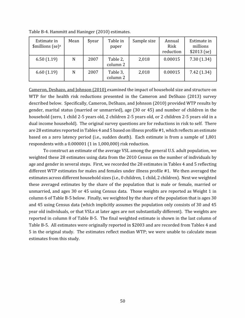
50

Table B-4. Hammitt and Haninger (2010) estimates.

Estimate in $millions (se)a

Mean $year Table in paper

Sample size Annual Risk

reduction

Estimate in millions

$2013 (se) 6.50 (1.19) N 2007 Table 2,

column 2 2,018 0.00015 7.30 (1.34)

6.60 (1.19) N 2007 Table 3, column 2

2,018 0.00015 7.42 (1.34)

Cameron, Deshazo, and Johnson (2010) examined the impact of household size and structure on WTP for the health risk reductions presented in the Cameron and DeShazo (2013) survey described below. Specifically, Cameron, DeShazo, and Johnson (2010) provided WTP results by gender, marital status (married or unmarried), age (30 or 45) and number of children in the household (zero, 1 child 2-5 years old, 2 children 2-5 years old, or 2 children 2-5 years old in a dual income household). The original survey questions are for reductions in risk to self. There are 28 estimates reported in Tables 4 and 5 based on illness profile #1, which reflects an estimate based on a zero latency period (i.e., sudden death). Each estimate is from a sample of 1,801 respondents with a 0.000001 (1 in 1,000,000) risk reduction.

To construct an estimate of the average VSL among the general U.S. adult population, we weighted these 28 estimates using data from the 2010 Census on the number of individuals by age and gender in several steps. First, we recorded the 28 estimates in Tables 4 and 5 reflecting different WTP estimates for males and females under illness profile #1. We then averaged the estimates across different household sizes (i.e., 0 children, 1 child, 2 children). Next we weighted these averaged estimates by the share of the population that is male or female, married or unmarried, and ages 30 or 45 using Census data. Those weights are reported as Weight 1 in column 6 of Table B-5 below. Finally, we weighted by the share of the population that is ages 30 and 45 using Census data (which implicitly assumes the population only consists of 30 and 45 year old individuals, or that VSLs at later ages are not substantially different). The weights are reported in column 8 of Table B-5. The final weighted estimate is shown in the last column of Table B-5. All estimates were originally reported in $2003 and are recorded from Tables 4 and 5 in the original study. The estimates reflect median WTP; we were unable to calculate mean estimates from this study.

51

Table B-5. Cameron, DeShazo, and Johnson (2010) estimates.

Estimate in $millions

(se)a

Gender Kids Age Estimate in millions

$2013 (se)

Weight 1 Weighted estimate 1b

Weight 2 Weighted estimate 2 in

$2013 (se) 8.81 (1.93) Male,

married 0 30 11.15 (2.45) 0.261 9.10 (2.20) 0.495 7.640 (1.75)

11.01 (2.40) 1 13.94 (3.04) 13.16 (3.25) 2 16.66 (4.11) 6.56 (1.74) Male,

unmarried 0 8.31 (2.21) 0.231

8.74 (2.16) 1 11.07 (2.74) 10.91 (3.04) 2 13.81 (3.85) 3.59 (0.74) Female,

married 0 4.55 (0.94) 0.293

4.50 (0.88) 1 5.70 (1.12) 5.42 (1.23) 2 6.86 (1.56) 6.26 (1.45) 2, dual-

income 7.93 (1.83)

2.62 (0.69) Female, unmarried

0 3.32 (0.88) 0.214 3.55 (0.86) 1 4.49 (1.09) 4.45 (1.22) 2 5.63 (1.54) 5.14 (1.47) 2, dual-

income 6.51 (1.85)

9.56 (1.74) Male, married

0 45 12.10 (2.21) 0.323 6.20 (1.31) 0.505 5.61 (1.03) 1 7.10 (1.30) 3.57 (0.92) 2 4.52 (1.17) 7.33 (1.52) Male,

unmarried 0 9.28 (1.92) 0.167

4.09 (0.92) 1 5.18 (1.17)

52

2.42 (0.88) 2 3.06 (1.11) 3.96 (0.57) Female,

married 0 5.01 (0.72) 0.335

2.83 (0.45) 1 3.58 (0.57) 2.01 (0.50) 2 2.54 (0.64) 2.18 (0.56) 2, dual-

income 2.76 (0.70)

3.04 (0.52) Female, unmarried

0 3.85 (0.66) 0.263 2.06 (0.43) 1 2.61 (0.55) 1.34 (0.51) 2 1.70 (0.65) 1.42 (0.78) 2, dual-

income 1.80 (0. 72)

a. Standard errors are calculated using information on the confidence intervals associated with the estimates provided in Cameron, DeShazo, and Johnson (2010).

b. Weighted estimate 1 = average of male/female, married/unmarried estimates*weight 1.

PRELIMINARY DRAFT: All results provisional and subject to change.

53

Cameron, DeShazo, and Stiffler (2013) used data from the Cameron and DeShazo (2013) survey to compare estimates from the U.S. to those from a companion survey conducted in Canada using the same survey and mode. We used estimates from the U.S. sample only. Cameron, DeShazo, and Stiffler (2013) reported a series of estimates based on a “sudden death simulation” for different ages (25, 35 and 65) and gender, resulting in 6 estimates from this study. Estimates were reported on pages 268 and 269 in the original study in $2003. We weighted the estimates in the same manner as used for the study by Cameron, DeShazo, and Johnson (2010) described above. Using 2010 Census data we were able to weight by age and gender (no averaging was needed). All estimates are based on an average household income of $42,000 and reflect median WTP. We do not have sufficient information to calculate the mean estimates.

We approximated the standard errors of the weighted VSL estimates the graphical information provided in an on-line appendix referenced in Figure 3 of the original study. We enlarged each graphic to visually identify an approximate point estimate for the 5th and 95th percentiles associated with each WTP estimate. We then used this information to calculate a standard error for each estimate.

Table B-6. Cameron, DeShazo, and Stiffler (2013) estimates.

Estimate in

$millions (se)

Age Gender Refer-ence in original

study

Sample size

Annual Risk

reduct-ion

Estimate in millions

$2013 (se)

Weight Weighted estimate

in millions $2103

(se) 9.36

(3.04) 25 M p 269 1801 10-6 11.85

(3.85) 0.196 8.58

(2.22) 10.46 (2.22)

35-50

M p 268 1801 10-6 13.24 (2.82)

0.175

5.83 (2.09)

65 M p 269 1801 10-6 7.38 (1.92)

0.124

5.01 (2.07)

25 F p 269 1801 10-6 6.34 (1.90)

0.190

5.72 (1.38)

35-40

F p 269 1801 10-6 7.24 (1.27)

0.176

3.08 (1.15)

65 F p 269 1801 10-6 3.90 (1.06)

0.138

Chestnut, Rowe, and Breffle (2012) examined differences in WTP estimates between the U.S. and Canada across different health endpoints (cancer and heart attack), risk reductions (1, 2, and 5

PRELIMINARY DRAFT: All results provisional and subject to change.

54

in 10,000) and question formats (choice question and payment card). We use the results for the U.S. sample only. The survey was administered to adults ages 35-85 using an internet survey (Knowledge Networks) in 2003. There were 885 respondents to the U.S. survey. Respondents were provided information on the type of fatal risk (cancer or heart attack), the annual risk reduction for the next 10 years, and then beyond 10 years, baseline risks, and costs for reductions. The authors used a grid as a visual aid to depict risk reductions. The risk reduction occurred via a health care program that had no side effects and would need to be paid for annually out of pocket. Each respondent was asked four choice questions, followed by a payment card question. For each choice question the respondent chose between two scenarios and then subsequently chose between the selected scenario and a status quo. We used 12 estimates from this study, as shown in Table B-7. We also used the reported 95% confidence intervals to calculate standard errors for the VSL estimates. The coefficient on the size of the risk reduction was significantly different from zero, but did not indicate a proportional response in WTP to the size of the risk.

Table B-7. Chestnut, Rowe, and Breffle (2012) estimates.

Estimate in $millions

(se)

$year Mean Reference in

original study

Sample size

Risk reduction

Health Endpoint

Estimate in millions

$2013 (se)

8.09 (0.64) 2002 Y Table 9 845 0.0001 Cancer 10.48 (.083) 5.04 (0.33) 2002 Y Table 9 845 0.0002 Cancer 6.53 (0.43) 2.80 (0.18) 2002 Y Table 9 845 0.0005 Cancer 3.63 (0.23) 7.17 (0.71) 2002 Y Table 9 845 0.0001 Heart attack 9.28 (0.92) 4.58 (0.41) 2002 Y Table 9 845 0.0002 Heart attack 5.93 (0.53) 2.62 (0.26) 2002 Y Table 9 845 0.0005 Heart attack 3.39 (0.33) 3.78 (0.31) 2002 Y Table 10 845 0.0001 Cancer 4.89 (0.4) 2.21 (0.15) 2002 Y Table 10 845 0.0002 Cancer 2.86 (0.20) 1.42 (0.15) 2002 Y Table 10 845 0.0005 Cancer 1.84 (0.20) 4.51 (0.43) 2002 Y Table 10 845 0.0001 Heart attack 5.84 (0.56) 2.64 (0.28) 2002 Y Table 10 845 0.0002 Heart attack 3.42 (0.36) 1.70 (0.31) 2002 Y Table 10 845 0.0005 Heart attack 2.20 (0.40)

Cameron and DeShazo (2013) is the “flagship” paper from the Cameron and DeShazo series of studies used in our analysis. This stated preference survey elicited WTP for a host of morbidity and mortality health endpoints that varied according to latency, type of cancer (breast, prostate, lung, colon, and skin), other diseases (heart attack, heart disease, stroke, respiratory illness,

PRELIMINARY DRAFT: All results provisional and subject to change.

55

diabetes, Alzheimer’s disease), automobile accidents, period of illness and recovery, if any, etc. Respondents could reduce their risks through the purchase of new programs that would change (improve) the specific illness profile. The new programs involved blood tests and lifestyle changes and possible drug therapies. The survey was administered to a representative sample of the general population of adults using an internet survey mode (Knowledge Networks); 1,801 individuals responded to the survey. Respondents were presented with five different choice scenarios and each scenario had three alternatives (two programs and the status quo). In an Appendix (B), the authors examined a number of scope and validity tests for their estimates and concluded that responses are sensitive to the magnitude of the risk reduction, although not always in a proportional manner.

We used nine estimates of the VSL for specific sub-populations from Cameron and DeShazo (2013) to calculate four estimates of the average VSL among the general U.S. adult population, as indicated in Table B-8. The first four estimates were weighted with the each of the last five estimates such that sixe estimates were used to calculate each weighted average. The estimates from the study reflect different ages, income levels, and discount rates. We could not determine a reasonable way to combine estimates across discount rates; therefore, we chose to weight each of the different age and income estimates by the four discount rates included in the study.

Table B-8. Cameron and DeShazo (2013) estimates.

Estimate in $millions

(se)

Discount rate

Age Income

Reference in original

study

Estimate in millions

$2013 (se)

Weight Weighted estimate in

millions $2013 (se)

8.33 (2.43) 0.03 45 $42,000 Table 2, column 3,

row 1

10.79 (3.08)

0.165 7.49 (3.22)

6.74 (2.30) 0.05 45 $42,000 Table 2, column 4,

row 1

8.53 (2.91) 0.165 7.12 (3.19)

5.48 (2.49) 0.07 45 $42,000 Table 2, column 5,

row 1

6.94 (3.15) 0.165 6.86 (3.23)

6.82 (2.91) Individual

45 $42,000 Table 2, column 6,

row 1

8.63 (3.69) 0.165 7.14 (3.32)

PRELIMINARY DRAFT: All results provisional and subject to change.

56

4.81 (1.72) 0.05 45 $25,000 Table 3, column 3,

row 1

6.09 (2.18) 0.148

9.26 (2.99) 0.05 45 $67,500 Table 3, column 5,

row 1

11.72 (3.78)

0.155

6.73 (2.23) 0.05 45 $42,000 (none if

sick)

Table 3, column 5,

row 1

8.52 (2.83) 0.175

0.72 (3.11) 0.05 35 $42,000 Table 4, column 2,

row 1

0.91 (3.93) 0.182

5.91 (2.62) 0.05 65 $42,000 Table 4, column 2,

row 7

7.48 (3.32) 0.178

Viscusi, Huber, and Bell (2014) conducted a stated preference survey designed to investigate whether people are willing to pay more to reduce cancer mortality risks than for reductions in mortality risks from other sources. A random sample of U.S. residents were asked about their preferences for hypothetical government policies that would reduce the risk of bladder cancer from drinking water contaminated by arsenic at some cost to their household. The survey described exposure routes and symptoms of bladder cancer and indicated that symptoms typically occur 10 years after developing the disease. An iterative choice question format was used to elicit willingness to pay. Baseline risks were either 2 or 4 out of 100,000 annually. The hypothesized risk reduction was either 2, 3, or 4 out of 100,000. There were 3,420 respondents in the internet-based survey (Knowledge Networks), which was administered to individuals of age 18 and older in 2008 and 2009. The authors applied a 3% discount rate to the results from all three choice questions to obtain estimates for an immediate risk reduction.

We calculated standard errors for the reported VSL estimates using the confidence intervals reported by the authors for the undiscounted estimates. The confidence intervals are small, indicating that the estimates are very precise. In terms of validity, the authors do not explicitly address tests. However, regression results indicate that respondents are willing to pay more for treatment that reduces risk to zero.

PRELIMINARY DRAFT: All results provisional and subject to change.

57

Table B-9. Viscusi, Huber, and Bell (2014) estimates.

Estimate in $millions (se)

Mean $year Reference in original study

Sample size Annual Risk

reduction

Estimate in millions

$2013 (se) 10.85 (0.085) Y 2011 Page 394 in

text 3430 0.000001 11.24 (0.09)

15.96 (0.126) Y 2011 calculateda 3430 0.000001 16.53 (0.13)

a. In footnote 16 of VHB the authors provide the “benefit increase factor” for a 7% discount rate which we use to calculate a VSL.

Hedonic wage studies

Viscusi (2003) constructed job fatality risk measures separately for black and white workers based on BLS CFOI data collected between 1992-1997 to test for systematic differences in compensating wage differentials by race. The mortality risk variables for the analysis were distinguished by race and by two digit SIC code industry groups. Worker data were drawn from the 1997 CPS MORG.

We draw our estimates from the “full sample” results reported Table 5 estimated separately by race using both ln(wage) and wage as the dependent variable. For each specification (log or level) we weighted the estimated VSLs by the proportion of the 2013 total US population identified as “white” or “black or African American” by the US Census. This produced two population-weighted VSL estimates for our analysis.

We computed standard errors for the VSL estimates using the robust clustered standard errors reported for the risk coefficient, appropriately adjusted for population weighting. Note that because the estimating equation is log-linear the VSL and its standard error also depend, respectively, on the wage rate and its standard error (Aldy and Viscusi 2008). Following Viscusi (2015), where standard errors of the VSL are not provided in the original study we constructed them based on the standard errors of the risk coefficient alone. Controls in the regressions included non-fatal injury and illness rate, public employment, nine occupational groups, industry controls for construction and manufacturing, and several demographic variables.

Table B-10. Viscusi (2003) estimates.

Estimate in $millions (se)

Mean $year Table in

paper

Sample size

Estimate in millions

$2013 (se)

Weight Weighted Estimate in

millions $2013 (se)

15.0 (7.64) Y 2002 5 83625 19.42 (9.90) 0.855 17.96 (8.49) 7.2 (3.48) Y 2002 5 9735 9.32 (4.51) 0.155

13.4 (7.06) Y 2002 5 83625 17.35 (9.14) 0.855 16.58 (7.86)

PRELIMINARY DRAFT: All results provisional and subject to change.

58

9.3 (4.08) Y 2002 5 9735 12.04 (5.28) 0.155 Viscusi (2004) estimated values for both a full sample and several subsamples of workers. The source of the risk data is BLS CFOI 1992-1997 and the risk measure is based on the workers industry-occupation group. Worker data are full-time, nonagricultural workers age 18-65 who are not in the armed forces from the 1997 CPS MORG.

We drew estimates from the full sample results reported Table 3, which presents separate VSL estimates based on a 1992-1997 averaged mortality risk and using only 1997 risk. The results are further differentiated by log-linear and linear specifications, resulting in four different VSL estimates. The analysis included controls for non-fatal injury and illness, nine occupational classifications, public sector employment, and an array of demographic factors. Because the results were based on the full sample we did not apply any population weights. We calculated standard errors for the VSL estimates using the reported standard errors for the risk coefficients.

Table B-11. Viscusi (2004) estimates.

Estimate in $millions (se)

Mean $year Table in paper

Sample size

Estimate in millions

$2013 (se)

Weighted estimate in

millions $2013 (se)

4.2 (2.24) Y 1997 3 99033 6.10 (3.25) n/a 2.5 (1.97) Y 1997 3 99033 3.63 (2.86) 4.7 (2.76) Y 1997 3 99033 6.82 (4.01) 2.6 (2.38) Y 1997 3 99033 3.77 (3.45)

Kneisner and Viscusi’s (2005) examined the impact on the estimated VSL from relative position on the wage distribution and relative age. The source of the fatal risk measures was BLS CFOI data collected between1992-1997 and the risk measure was based on each worker’s industry-occupation group. Data on workers are non-agricultural full-time workers between the ages of 18 and 65 from the CPS MORG files for 1997.

We drew VSL estimates from the “Full Sample” portion of Table 1, labeled (ii) and (iii) in the original study. Estimate (i) from the study is also a full sample estimate but appears to be replicated, for comparison purposes, from Viscusi (2004), which we included elsewhere. The analysis included controls for injury and illness rate, nine occupational dummy variables, and a host of demographic variables.

Standard errors for the VSL should be constructed by using the standard errors of the risk coefficient, wage, the coefficient of the interacted wage rank * fatality risk variable, and the

PRELIMINARY DRAFT: All results provisional and subject to change.

59

standard deviation of this constructed variable. However, because some of this information was not available, we constructed standard errors for the VSL estimates using the reported standard errors of the risk coefficients alone. Because this was a full sample study we did not apply any population weighting to these estimates.

Table B-12. Kneisner and Viscusi (2005) estimates

Estimate in $millions (se)

Mean $year Table in paper

Sample size

Estimate in millions

$2013 (se)

Weighted Estimate in

millions $2013 (se)

3.46 (.58) Y 1997 1 99033 5.02 (.084) n/a 3.57 (.55) Y 1997 1 99033 5.18 (0.80)

Viscusi and Aldy (2007) examined the age variation in the VSL based on variation in job risks by industry and worker age. Fatality risks were calculated using data from the BSL CFOI for the years 1992-1997, which was constructed by two- or three-digit industry SIC codes and five age groups spanning a range from 18 to 62 years old. Worker data were obtained from the 1998 CPS MORG data file with a number of screens. The sample excluded agricultural workers and members of the armed forces, those with less than a 9th grade education, workers with implicit hourly wages less than the minimum wage, and less than full time workers.

We drew our estimates from Table 2, Panel B where risks are specific to age-industry groups and there are controls for nonfatal injury risks. VSL estimates were provided separately for each of five age groups. We constructed a single adult VSL by weighting these VSLs by the respective proportion of the age group to the entire population aged 18-62 in 2013. We computed standard errors for the VSL estimates using the reported robust clustered standard errors for the risk coefficients, appropriately adjusted for population weighting. The authors noted that there is a covariance term across the age-specific VSL estimates, but we lack the data to incorporate this into the calculated standard error for the weighted VSL. The VSL estimates are based upon ln(wage) as the dependent variable and the specifications we draw upon include controls for non-fatal injury rates by industry and age group, nine occupation indicators, regional, and demographic variables.

Table B-13. Viscusi and Aldy (2007) Estimates

Estimate in $millions (se)

Mean $year Table in

paper

Sample size

Estimate in millions

$2013 (se)

Weight Weighted Estimate in

millions $2013 (se)

6.45 (1.47) Y 2002 2 120008 8.73 (1.99) 0.125 8.61 (1.20)

PRELIMINARY DRAFT: All results provisional and subject to change.

60

6.72 (1.63) Y 2002 2 9.09 (2.21) 0.236 8.99 (2.08) Y 2002 2 12.16 (2.82) 0.222 5.42 (2.05) Y 2002 2 7.33 (2.78) 0.241 3.81 (2.17) Y 2002 2 5.15 (2.93) 0.176

Aldy and Viscusi (2008) used an age-dependent fatal risk measure to estimate age-specific hedonic wage regressions. The source of the fatal risk measures was the BLS CFOI data for 1992-2000 and the risk measures were conditional upon a worker’s age group and two-digit SIC industry. Data on workers were obtained from the CPS Merged Outgoing Rotation Group (MORG) files for 1993-2000, aged 18 to 62. These data exclude agricultural workers, members of the armed forces, workers making less than minimum wage, less than full-time workers, and those with top-coded income. The analysis controlled for nonfatal injury risk and expected worker’s compensation rate in addition to indicator variables for one-digit occupation, region of residence, public sector employment, and an array of demographic characteristics.

We drew our estimates from Table 1. Mean VSL estimates for each year were constructed by weighting the age-group specific VSL estimates. Weights are the proportion of each age group in the total population of persons aged 18-62, taken from the proportion of the total age 18-62 population in these age groups in 2013. This resulted in seven VSL estimates from this study, each taken as value from a distinct sample.

We computed standard errors for the VSL estiamtes using the standard errors reported for the risk coefficients from the wage equations, adjusted using the population weights. In computing these standard errors, were were not able to account for the covariance across age-specific VSL estimates.

Table B-14. Aldy and Viscusi (2008) estimates

Estimate in $millions (se)

Mean $year Table in

paper

Sample size

Estimate in millions

$2013 (se)

Weight Weighted Estimate in

millions $2013 (se)

0.95 (0.87) Y 2000 1 123439 (assumed)

1.29 (1.17) 0.125 7.10 (1.15) 9.95 (1.69) Y 2000 13.46 (2.29) 0.236 8.29 (2.14) Y 2000 11.21 (2.89) 0.222 1.79 (1.76) Y 2000 2.42 (2.39) 0.241 2.91 (2.18) Y 2000 3.94 (2.95) 0.176 4.54 (.64) Y 2000 123439

(assumed) 6.14 (0.86) 0.125 7.40 (1.19)

7.42 (1.48) Y 2000 10.04 (2.01) 0.236

PRELIMINARY DRAFT: All results provisional and subject to change.

61

7.09 (2.05) Y 2000 9.59 (2.77) 0.222 3.4 (2.24) Y 2000 4.60 (3.03) 0.241 4.3 (2.18) Y 2000 5.82 (2.94) 0.176

4.57 (1.01) Y 2000 123439 (assumed)

6.18 (1.36) 0.125 7.11 (1.19) 6.98 (1.49) Y 2000 9.44 (2.01) 0.236 5.68 (2.12) Y 2000 7.68 (2.86) 0.222 4.69 (2.15) Y 2000 6.34 (2.91) 0.241 3.67 (2.2) Y 2000 4.96 (2.98) 0.176

4.53 (1.48) Y 2000 123439 (assumed)

6.13 (2.00) 0.125 7.47 (1.20) 7.36 (1.51) Y 2000 9.96 (2.05) 0.236 8.04 (2.33) Y 2000 10.88 (3.16) 0.222 3.93 (2.08) Y 2000 5.32 (2.81) 0.241 2.77 (1.86) Y 2000 3.75 (2.52) 0.176 5.48 (1.34) Y 2000 123439

(assumed) 7.41 (1.81) 0.125 8.68 (1.21)

7.52 (1.66) Y 2000 10.17 (2.24) 0.236 8.62 (2.04) Y 2000 11.66 (2.76) 0.222 5.4 (2.08) Y 2000 7.31 (2.81) 0.241 4.23 (2.3) Y 2000 5.72 (3.11) 0.176

6.45 (1.46) Y 2000 123439 (assumed)

8.73 (1.98) 0.125 8.61 (1.19) 6.72 (1.62) Y 2000 9.09 (2.19) 0.236 8.99 (2.07) Y 2000 12.16 (2.80) 0.222 5.42 (2.05) Y 2000 7.33 (2.78) 0.241 3.81 (2.12) Y 2000 5.15 (2.87) 0.176 3.43 (.082) Y 2000 123439

(assumed) 4.64 (1.10) 0.125 9.30 (1.07)

7.45 (1.45) Y 2000 10.08 (1.97) 0.236 9.13 (2.09) Y 2000 12.35 (2.82) 0.222 8.7 (1.95) Y 2000 11.77 (2.63) 0.241 3.2 (1.48) Y 2000 4.33 (2.01) 0.176

3.74 (1.07) Y 2000 123439 5.06 (1.45) 0.125 9.99 (1.27) 9.43 (1.69) Y 2000 12.76 (2.28) 0.236 9.66 (2.44) Y 2000 13.07 (3.30) 0.222 8.07 (2.11) Y 2000 10.92 (2.86) 0.241 3.43 (2.24) Y 2000 4.64 (3.03) 0.176

PRELIMINARY DRAFT: All results provisional and subject to change.

62

Viscusi and Hersch (2008) examined the mortality cost of smoking (to smokers themselves) by using hedonic wage data to estimate the VSL by smoking status. Workplace fatality rates were calculated from BLS CFOI data by industry-age-gender for the years 1996-2001, weighted by hours worked. This resulted in gender-specific fatality risk measures by two-digit industry groups in five age groups, which range from 20 to 64 years old. Worker data were obtained from the monthly CPS survey and the CPS Tobacco Use Supplements conducted in 1995-1996, 1998-1999, and 2001-2002.

We drew our estimates from Table 2, Panel A where the dependent variable was ln(wage) and there were no age variations in risk coefficients. The VSL was estimated separately for smoker and non-smoker samples. We weighted these separate estimates by the proportions of adults who did and did not smoke in 2012, as estimated by the Centers for Disease Control, to produce an estimate of the average VSL for the general U.S. adult population. We computed standard errors for the VSL from robust clustered standard errors reported for the risk coefficient estimates, appropriately adjusted for the population weighting. Controls included non-fatal injury rate, ten occupation groups, government employment, and demographic characteristics.

Table B-15. Viscusi and Hersch (2008) estimates.

Estimate in $millions (se)

Mean $year Table in

paper

Sample size

Estimate in millions

$2013 (se)

Weight Weighted Estimate in

millions $2013 (se)

7.39 (3.36) Y 2000 2 212067 10.00 (4.54) 0.819 9.98 (3.81)

7.32 (3.38) Y 2000 2 66844 9.90 (4.57) 0.181

Hersch and Viscusi (2010) examined the effect of immigrant status on risk compensation in the labor market. We drew values from a specification based on fatality rates calculated using data from BLS CFOI between 2003-2005, calculated by two-digit industry, immigrant status, and age (by two age groups). Worker data for these values were obtained from the 2003 CPS MOR, restricted to 1.) workers in occupations that had been characterized as blue-collar jobs in prior versions of the CPS, 2.) those who were net self-employed, 3.) earned hourly wages between $1.50 and $100, and 4.) were between the ages of 18 and 64.

Column 3 of Table 3 contains the specification that provided the single value we extracted from this study. This specification included both immigrant and native U.S. workers, controlled for non-fatal injury, immigrant status, immigrant–risk interactions, occupation, government employment, and other factors. As reported on page 762, the estimated VSL for native U.S. workers was $7.95 million ($2003), while the estimated VSL was negative for immigrant workers. An overall VSL for the entire sample was not reported. We use the value for U.S.

PRELIMINARY DRAFT: All results provisional and subject to change.

63

workers only, accepting it as sufficiently representative to be included in our analysis, and do not incorporate the negative implied VSL for immigrants. We computed a standard error for the VSL estimate using the standard error reported for the risk coefficient. The study provided other specifications for sensitivity analysis but none of these controlled for non-fatal injury.

Table B-16. Hersch and Viscusi (2010) estimates.

Estimate in $millions (se)

Mean $year Table in paper

Sample size

Estimate in millions

$2013 (se)

Weighted Estimate in

millions $2013 (se)

7.95 (6.53) Y 2003 3 61437 10.07 (8.27) n/a Scotten and Taylor (2011) developed estimates of the VSL based on risk rates that were differentiated by how the fatal injury occurred. These fatality rates were constructed using BLS CFOI data collected between 1992 and 1997. Occupations were aggregated into 22 categories and industries into 23 categories, and the risk measure was based on a worker’s industry-occupation group. The authors screened risk data to include only deaths that were likely to be considered as part of a wage-negotiation between employee and employer. Risk rates also were created for three major categories of death: traditional accidental deaths, transportation-related deaths, and violent assaults. Worker data were obtained from CPS MORG for years between 1996 and 1998, limited to the high-wage segment of the labor market. Compared to broader CPS samples, this resulted in a sample with a higher proportion of workers holding an undergraduate degree; are white, male, and married; and that live in a large metropolitan area.

We drew our estimates from Table 3, which includes results from the full sample with risks undifferentiated by type. The authors reported the standard error of the VSL estimates, so no auxiliary calculations were needed. The analysis controlled for non-fatal injury risk (at the industry level), a range of industry and occupation groups, and a host demographic variables. The authors also reported results for differentiated risks and for subsamples, but we relied solely upon the broader-based estimates for comparability with the other primary VSL estimates in our meta-dataset.

Table B-17. Scotton and Taylor (2011) estimates.

Estimate in $millions (se)

Mean $year Table in paper

Sample size

Estimate in millions

$2013 (se)

Weighted Estimate in

millions $2013 (se)

8.7 (2.88) Y 1997 3 43261 12.63 (4.18) n/a

9.9 (2.58) Y 1997 3 43261 14.37 (3.74)

PRELIMINARY DRAFT: All results provisional and subject to change.

64

5.8 (1.78) Y 1997 3 43261 8.42 (2.58)

Scotton (2013) examined the sensitivity of the VSL to a number different choices in constructing the risk variable from BLS CFOI data as well as the specification of the hedonic wage equation. In all cases the source of the risk data was the BLS CFOI dataset. Worker data were obtained from the 2006 CPS MORG dataset and pertain to full-time, nonfarm, payroll labor participants between the ages of 16 and 72. While some results in the study relied upon a restricted subsample of these data, the estimates we extracted used the entire sample.

We drew estimates from Table 2 of the study, excluding the first column which reports estimates from Viscusi (2004). The remaining estimates in the table were divided into two sets based on whether the dependent variable was ln(wage) or wage. Within these sets there were six different constructions for risk, representing alternative occupation and industry pairings. We used all of these alternatives for a total of twelve primary VSL estimates from the study. The models included occupational controls, but no controls for public vs private industry. The models also did not control for non-fatal injury because those measures were only available by industry or occupation. However, the author noted that “including one or both of these non-fatal rates long with the various industrial and occupational controls adds little and changes nothing about the results of this study,” although that observation may be specific to conclusions about construction of the risk variable and choice of occupation-industry controls rather than the magnitude of the VSL itself.

The study presented additional regression results in Table 4, based on models where the number of industry and occupation controls were varied in a log-linear model for two different risk measures. Specifications ranged from no industry or occupation controls to 73 industry and 21 occupation controls. The author did not report VSL estimates but did report risk coefficients for these models. We constructed VSL estimates from the specifications in column 4, which included both industry and occupation controls. We also constructed VSL estimates from the regression results reported in Table 5, where the specification included more extensive industry and occupation controls. In both cases we used the mean wage for the “restricted sample” reported in Table 1. We computed standard errors for the VSL estimates from the standard error reported for the risk coefficients. All of the estimates extracted from this study are “full sample” results that did not require any population-weighting.

Table B-18. Scotton (2013) estimates.

Estimate in $millions (se)

Mean $year Table in

paper

Sample size

Estimate in millions

$2013 (se)

Weighted Estimate in

millions $2013 (se)

PRELIMINARY DRAFT: All results provisional and subject to change.

65

15.95 (3.85) Y 2006 2 121608 18.43 (4.45) n/a 18.17 (3.70) Y 2006 2 121608 20.99 (4.28) 13.47 (4.48) Y 2006 2 121608 15.56 (5.17) 11.36 (3.03) Y 2006 2 121608 13.13 (3.51) 12.88 (3.18) Y 2006 2 121608 14.88 (3.68) 11.17 (2.92) Y 2006 2 121608 12.91 (3.38) n/a 12.47 (4.19) Y 2006 2 121608 14.41 (4.84) 14.76 (3.91) Y 2006 2 121608 17.06 (4.52) 10.57 (4.76) Y 2006 2 121608 12.21 (5.50) 8.14 (3.37) Y 2006 2 121608 9.41 (3.90) 9.64 (3.55) Y 2006 2 121608 11.14 (4.10) n/a 8.09 (3.28) Y 2006 2 121608 9.35 (3.79)

14.71 (4.23) Y 2006 3 84336 16.99 (4.89) 15.23 (2.96) Y 2006 3 84336 17.60 (3.42) 16.58 (4.15) Y 2006 3 84336 19.16 (4.80) 17.06 (2.92) Y 2006 3 84336 19.72 (3.37) n/a 12.57 (3.97) Y 2006 3 84336 14.53 (4.58) 13.88 (2.43) Y 2006 3 84336 16.04 (2.81) 5.50 (2.96) Y 2006 4 84336 6.36 (3.42) 6.02 (2.96) Y 2006 4 84336 6.96 (3.42) 7.82 (2.36) Y 2006 4 84336 9.04 (2.72) n/a 6.59 (2.51) Y 2006 4 84336 7.61 (2.90) 7.56 (2.51) Y 2006 4 84336 8.73 (2.90) 8.12 (1.83) Y 2006 4 84336 9.38 (2.12)

PRELIMINARY DRAFT: All results provisional and subject to change.

66

References

Brady KL. 2008. An expressed preference determination of college students’ valuation of statistical lives: methods and implications. College Student Journal 42(4): 968-981.

Carson RT, Mitchell RC. 2006. Risk preferences toward environmental risks: the case of trihalomethanes. In Alberini A, Kahn JR, eds. Handbook on Contingent Valuation. Massachusetts: Edward Elgar.

Hakes JK, Viscusi WK. 2007. Automobile seatbelt usage and the value of statistical life. Southern Economic Journal 73(3): 659-676.

Ludwig J, Cook PJ. 2001. The benefits of reducing gun violence: evidence from contingent-valuation survey data. Journal of Risk and Uncertainty 22(3): 207-226.

Morris J, Hammitt JK. 2001. Using life expectancy to communicate benefits of health care programs in contingent valuation studies. Health Economics Nov-Dec: 468-478.

PRELIMINARY DRAFT: All results provisional and subject to change.

67

Appendix C This appendix contains results from sensitivity analysis over the assumed income elasticity of the VSL.

Table C-1. Non-parametric estimates of the average VSL among the U.S. adult general population [2013$/statistical life/yr]. Income elasticity = 0.1.

Estimator mm/ma HWb SP pooled balanced

1 simple mean mm 11.3 [ 1.43 ]c 6.96 [ 0.907 ] 9.24 [ 1.27 ] 9.14 [ 0.843 ]

m 11.3 [ 1.43 ] 7.93 [ 1.70 ] 10.0 [ 1.37 ] 9.63 [ 1.00 ]

2 mean of group means

mm 9.36 [ 0.423 ] 7.25 [ 0.672 ] 8.23 [ 0.441 ] 8.31 [ 0.396 ]

m 9.36 [ 0.423 ] 9.44 [ 1.03 ] 9.40 [ 0.550 ] 9.40 [ 0.506 ]

3 sample size weighted mean

mm 11.3 [ 1.56 ] 7.53 [ 1.23 ] 11.2 [ 1.56 ] 9.39 [ 0.996 ]

m 11.3 [ 1.56 ] 8.18 [ 1.81 ] 11.2 [ 1.57 ] 9.72 [ 1.09 ]

4 sampling var. weighted mean

mm 8.28 [ 1.03 ] 6.16 [ 2.83 ] 6.20 [ 2.76 ] 7.22 [ 1.51 ]

m 8.28 [ 1.03 ] 8.92 [ 3.21 ] 8.90 [ 3.00 ] 8.60 [ 1.71 ]

5 total var. weighted mean

mm 9.15 [ 0.447 ] 6.57 [ 0.773 ] 7.90 [ 0.615 ] 7.86 [ 0.446 ]

m 9.15 [ 0.447 ] 7.67 [ 1.18 ] 8.71 [ 0.654 ] 8.41 [ 0.628 ]

a. “mm” includes mean and median primary estimates, “m” includes only mean primary estimates. b. The “mm” and “m” HW estimates in the first column of numbers are identical because HW studies only

reported mean VSL estimates. c. Numbers is square brackets are bootstrapped standard errors.

PRELIMINARY DRAFT: All results provisional and subject to change.

68

Table C-2. Non-parametric estimates of the average VSL among the U.S. adult general population [2013$/statistical life/yr]. Income elasticity = 0.5.

Estimator mm/ma HWb SP pooled balanced

1 simple mean mm 11.7 [ 1.24 ]c 7.34 [ 0.968 ] 9.62 [ 1.22 ] 9.52 [ 0.782 ]

m 11.7 [ 1.24 ] 8.36 [ 1.83 ] 10.4 [ 1.32 ] 10.0 [ 0.972 ]

2 mean of group means

mm 10.0 [ 0.392 ] 7.65 [ 0.702 ] 8.74 [ 0.456 ] 8.83 [ 0.400 ]

m 10.0 [ 0.392 ] 10.0 [ 1.10 ] 10.0 [ 0.575 ] 10.0 [ 0.526 ]

3 sample size weighted mean

mm 11.6 [ 1.36 ] 7.81 [ 1.25 ] 11.6 [ 1.37 ] 9.73 [ 0.924 ]

m 11.6 [ 1.36 ] 8.50 [ 1.84 ] 11.6 [ 1.37 ] 10.1 [ 1.03 ]

4 sampling var. weighted mean

mm 8.93 [ 1.02 ] 6.48 [ 2.95 ] 6.53 [ 2.87 ] 7.71 [ 1.56 ]

m 8.93 [ 1.02 ] 9.30 [ 3.28 ] 9.29 [ 3.07 ] 9.12 [ 1.74 ]

5 total var. weighted mean

mm 9.77 [ 0.408 ] 6.91 [ 0.809 ] 8.33 [ 0.633 ] 8.34 [ 0.453 ]

m 9.77 [ 0.408 ] 8.07 [ 1.25 ] 9.18 [ 0.666 ] 8.92 [ 0.655 ]

a. “mm” includes mean and median primary estimates, “m” includes only mean primary estimates. b. The “mm” and “m” HW estimates in the first column of numbers are identical because HW studies only

reported mean VSL estimates. c. Numbers is square brackets are bootstrapped standard errors.

PRELIMINARY DRAFT: All results provisional and subject to change.

69

Table C-3. Non-parametric estimates of the average VSL among the U.S. adult general population [2013$/statistical life/yr]. Income elasticity = 1.1.

Estimator mm/ma HWb SP pooled balanced

1 simple mean mm 12.4 [ 0.929 ]c 7.94 [ 1.07 ] 10.2 [ 1.15 ] 10.1 [ 0.706 ]

m 12.4 [ 0.929 ] 9.05 [ 2.04 ] 11.1 [ 1.26 ] 10.7 [ 0.961 ]

2 mean of group means

mm 11.1 [ 0.352 ] 8.30 [ 0.754 ] 9.59 [ 0.487 ] 9.70 [ 0.415 ]

m 11.1 [ 0.352 ] 11.0 [ 1.22 ] 11.1 [ 0.623 ] 11.1 [ 0.569 ]

3 sample size weighted mean

mm 12.3 [ 1.03 ] 8.28 [ 1.27 ] 12.2 [ 1.04 ] 10.3 [ 0.817 ]

m 12.3 [ 1.03 ] 9.02 [ 1.89 ] 12.2 [ 1.04 ] 10.6 [ 0.959 ]

4 sampling var. weighted mean

mm 9.96 [ 0.967 ] 6.98 [ 3.11 ] 7.03 [ 3.04 ] 8.47 [ 1.63 ]

m 9.96 [ 0.967 ] 9.87 [ 3.39 ] 9.87 [ 3.17 ] 9.91 [ 1.77 ]

5 total var. weighted mean

mm 10.8 [ 0.354 ] 7.46 [ 0.873 ] 9.01 [ 0.666 ] 9.12 [ 0.471 ]

m 10.8 [ 0.354 ] 8.73 [ 1.37 ] 9.92 [ 0.694 ] 9.76 [ 0.709 ]

a. “mm” includes mean and median primary estimates, “m” includes only mean primary estimates. b. The “mm” and “m” HW estimates in the first column of numbers are identical because HW studies only

reported mean VSL estimates. c. Numbers is square brackets are bootstrapped standard errors.

PRELIMINARY DRAFT: All results provisional and subject to change.

70

Table C-4. Non-parametric estimates of the average VSL among the U.S. adult general population [2013$/statistical life/yr]. Income elasticity = 1.4.

Estimator mm/ma HWb SP pooled balanced

1 simple mean mm 12.7 [ 0.775 ]c 8.26 [ 1.13 ] 10.6 [ 1.13 ] 10.5 [ 0.683 ]

m 12.7 [ 0.775 ] 9.43 [ 2.16 ] 11.5 [ 1.25 ] 11.1 [ 0.975 ]

2 mean of group means

mm 11.7 [ 0.342 ] 8.65 [ 0.784 ] 10.1 [ 0.507 ] 10.2 [ 0.426 ]

m 11.7 [ 0.342 ] 11.5 [ 1.28 ] 11.6 [ 0.652 ] 11.6 [ 0.598 ]

3 sample size weighted mean

mm 12.6 [ 0.845 ] 8.52 [ 1.28 ] 12.6 [ 0.860 ] 10.6 [ 0.769 ]

m 12.6 [ 0.845 ] 9.30 [ 1.92 ] 12.6 [ 0.856 ] 10.9 [ 0.933 ]

4 sampling var. weighted mean

mm 10.5 [ 0.929 ] 7.24 [ 3.20 ] 7.29 [ 3.12 ] 8.86 [ 1.67 ]

m 10.5 [ 0.929 ] 10.2 [ 3.45 ] 10.2 [ 3.22 ] 10.3 [ 1.79 ]

5 total var. weighted mean

mm 11.3 [ 0.334 ] 7.76 [ 0.909 ] 9.36 [ 0.686 ] 9.54 [ 0.486 ]

m 11.3 [ 0.334 ] 9.08 [ 1.45 ] 10.3 [ 0.714 ] 10.2 [ 0.742 ]

a. “mm” includes mean and median primary estimates, “m” includes only mean primary estimates. b. The “mm” and “m” HW estimates in the first column of numbers are identical because HW studies only

reported mean VSL estimates. c. Numbers is square brackets are bootstrapped standard errors.

PRELIMINARY DRAFT: All results provisional and subject to change.

71

Table C-5. Non-parametric estimates of the average VSL among the U.S. adult general population [2013$/statistical life/yr]. Income elasticity = 1.7.

Estimator mm/ma HWb SP pooled balanced

1 simple mean mm 13.1 [ 0.638 ]c 8.60 [ 1.20 ] 10.9 [ 1.10 ] 10.8 [ 0.675 ]

m 13.1 [ 0.638 ] 9.81 [ 2.28 ] 11.8 [ 1.25 ] 11.5 [ 1.01 ]

2 mean of group means

mm 12.3 [ 0.342 ] 9.02 [ 0.817 ] 10.5 [ 0.531 ] 10.7 [ 0.441 ]

m 12.3 [ 0.342 ] 12.1 [ 1.35 ] 12.2 [ 0.684 ] 12.2 [ 0.632 ]

3 sample size weighted mean

mm 13.0 [ 0.658 ] 8.77 [ 1.30 ] 12.9 [ 0.676 ] 10.9 [ 0.727 ]

m 13.0 [ 0.658 ] 9.58 [ 1.96 ] 12.9 [ 0.671 ] 11.3 [ 0.919 ]

4 sampling var. weighted mean

mm 11.0 [ 0.886 ] 7.51 [ 3.28 ] 7.56 [ 3.20 ] 9.26 [ 1.70 ]

m 11.0 [ 0.886 ] 10.4 [ 3.50 ] 10.5 [ 3.27 ] 10.7 [ 1.81 ]

5 total var. weighted mean

mm 11.9 [ 0.326 ] 8.07 [ 0.950 ] 9.73 [ 0.709 ] 9.98 [ 0.502 ]

m 11.9 [ 0.326 ] 9.45 [ 1.52 ] 10.7 [ 0.741 ] 10.7 [ 0.778 ]

a. “mm” includes mean and median primary estimates, “m” includes only mean primary estimates. b. The “mm” and “m” HW estimates in the first column of numbers are identical because HW studies only

reported mean VSL estimates. c. Numbers is square brackets are bootstrapped standard errors.

PRELIMINARY DRAFT: All results provisional and subject to change.

72

Table C-6. Maximum likelihood estimation results, income elasticity = 0.1. Coefficient estimates using only hedonic wage (HW) estimates, only stated preference (SP) estimates, HW and SP estimates combined with no control for study type (pooled), and HW and SP estimates combined with fixed effect for study type (balanced). Numbers in square brackets are standard errors.

Parameter HW SP pooled balanced

𝛽𝛽0 10.1 [ 0.534 ] 8.97 [ 0.991 ] 9.43 [ 0.664 ] 10.3 [ 0.923 ]

𝛽𝛽𝑦𝑦𝑠𝑠𝑚𝑚𝑦𝑦 1.94 [ 0.480 ] 1.37 [ 0.852 ] 1.41 [ 0.551 ] 1.60 [ 0.543 ]

𝛽𝛽𝑆𝑆𝑆𝑆 -0.152 [ 0.110 ]

𝛽𝛽𝑚𝑚𝑠𝑠𝑚𝑚𝑖𝑖𝑚𝑚𝑛𝑛 -0.470 [ 0.101 ] -0.467 [ 0.0848 ] -0.437 [ 0.0952 ]

𝜎𝜎𝜇𝜇 1.15 [ 0.551 ] 2.10 [ 0.325 ] 1.98 [ 0.267 ] 1.96 [ 0.268 ]

𝜎𝜎𝜂𝜂 0.517 [ 0.641 ] 2.42 [ 0.646 ] 2.03 [ 0.421 ] 1.86 [ 0.430 ]

𝑉𝑉𝑉𝑉𝑉𝑉𝐻𝐻𝐻𝐻 10.1 [ 0.534 ] 10.3 [ 0.923 ]

𝑉𝑉𝑉𝑉𝑉𝑉𝑆𝑆𝑆𝑆 8.97 [ 0.991 ] 8.71 [ 0.864 ]

𝑉𝑉𝑉𝑉𝑉𝑉𝑝𝑝𝑝𝑝𝑝𝑝𝑏𝑏𝑠𝑠𝑚𝑚 9.43 [ 0.664 ]

𝑉𝑉𝑉𝑉𝑉𝑉𝑏𝑏𝑚𝑚𝑏𝑏𝑚𝑚𝑛𝑛𝑏𝑏𝑠𝑠𝑚𝑚 9.48 [ 0.646 ]

PRELIMINARY DRAFT: All results provisional and subject to change.

73

Table C-7. Maximum likelihood estimation results, income elasticity = 0.5. Coefficient estimates using only hedonic wage (HW) estimates, only stated preference (SP) estimates, HW and SP estimates combined with no control for study type (pooled), and HW and SP estimates combined with fixed effect for study type (balanced). Numbers in square brackets are standard errors.

Parameter HW SP pooled balanced

𝛽𝛽0 10.5 [ 0.549 ] 9.42 [ 1.05 ] 9.88 [ 0.699 ] 10.7 [ 0.974 ]

𝛽𝛽𝑦𝑦𝑠𝑠𝑚𝑚𝑦𝑦 1.71 [ 0.471 ] 1.25 [ 0.900 ] 1.23 [ 0.580 ] 1.42 [ 0.572 ]

𝛽𝛽𝑆𝑆𝑆𝑆 -0.149 [ 0.112 ]

𝛽𝛽𝑚𝑚𝑠𝑠𝑚𝑚𝑖𝑖𝑚𝑚𝑛𝑛 -0.478 [ 0.101 ] -0.475 [ 0.0851 ] -0.447 [ 0.0951 ]

𝜎𝜎𝜇𝜇 1.27 [ 0.600 ] 2.19 [ 0.341 ] 2.07 [ 0.280 ] 2.05 [ 0.281 ]

𝜎𝜎𝜂𝜂 0.480 [ 0.810 ] 2.57 [ 0.683 ] 2.14 [ 0.446 ] 1.97 [ 0.455 ]

𝑉𝑉𝑉𝑉𝑉𝑉𝐻𝐻𝐻𝐻 10.5 [ 0.549 ] 10.7 [ 0.974 ]

𝑉𝑉𝑉𝑉𝑉𝑉𝑆𝑆𝑆𝑆 9.42 [ 1.05 ] 9.13 [ 0.909 ]

𝑉𝑉𝑉𝑉𝑉𝑉𝑝𝑝𝑝𝑝𝑝𝑝𝑏𝑏𝑠𝑠𝑚𝑚 9.88 [ 0.699 ]

𝑉𝑉𝑉𝑉𝑉𝑉𝑏𝑏𝑚𝑚𝑏𝑏𝑚𝑚𝑛𝑛𝑏𝑏𝑠𝑠𝑚𝑚 9.93 [ 0.679 ]

PRELIMINARY DRAFT: All results provisional and subject to change.

74

Table C-8. Maximum likelihood estimation results, income elasticity = 1.1. Coefficient estimates using only hedonic wage (HW) estimates, only stated preference (SP) estimates, HW and SP estimates combined with no control for study type (pooled), and HW and SP estimates combined with fixed effect for study type (balanced). Numbers in square brackets are standard errors.

Parameter HW SP pooled balanced

𝛽𝛽0 11.1 [ 0.573 ] 10.2 [ 1.14 ] 10.6 [ 0.758 ] 11.5 [ 1.06 ]

𝛽𝛽𝑦𝑦𝑠𝑠𝑚𝑚𝑦𝑦 1.32 [ 0.526 ] 1.03 [ 0.977 ] 0.911 [ 0.630 ] 1.11 [ 0.622 ]

𝛽𝛽𝑆𝑆𝑆𝑆 -0.145 [ 0.113 ]

𝛽𝛽𝑚𝑚𝑠𝑠𝑚𝑚𝑖𝑖𝑚𝑚𝑛𝑛 -0.489 [ 0.101 ] -0.487 [ 0.0854 ] -0.461 [ 0.0948 ]

𝜎𝜎𝜇𝜇 1.49 [ 0.696 ] 2.33 [ 0.365 ] 2.22 [ 0.300 ] 2.20 [ 0.301 ]

𝜎𝜎𝜂𝜂 0.368 [ 1.43 ] 2.82 [ 0.742 ] 2.33 [ 0.488 ] 2.16 [ 0.496 ]

𝑉𝑉𝑉𝑉𝑉𝑉𝐻𝐻𝐻𝐻 11.1 [ 0.573 ] 11.5 [ 1.06 ]

𝑉𝑉𝑉𝑉𝑉𝑉𝑆𝑆𝑆𝑆 10.2 [ 1.14 ] 9.83 [ 0.741 ]

𝑉𝑉𝑉𝑉𝑉𝑉𝑝𝑝𝑝𝑝𝑝𝑝𝑏𝑏𝑠𝑠𝑚𝑚 10.6 [ 0.758 ]

𝑉𝑉𝑉𝑉𝑉𝑉𝑏𝑏𝑚𝑚𝑏𝑏𝑚𝑚𝑛𝑛𝑏𝑏𝑠𝑠𝑚𝑚 10.7 [ 0.741 ]

PRELIMINARY DRAFT: All results provisional and subject to change.

75

Table C-9. Maximum likelihood estimation results, income elasticity = 1.4. Coefficient estimates using only hedonic wage (HW) estimates, only stated preference (SP) estimates, HW and SP estimates combined with no control for study type (pooled), and HW and SP estimates combined with fixed effect for study type (balanced). Numbers in square brackets are standard errors.

Parameter HW SP pooled balanced

𝛽𝛽0 11.4 [ 0.594 ] 10.6 [ 1.18 ] 11.0 [ 0.791 ] 11.9 [ 1.11 ]

𝛽𝛽𝑦𝑦𝑠𝑠𝑚𝑚𝑦𝑦 1.11 [ 0.592 ] 0.911 [ 1.02 ] 0.730 [ 0.657 ] 0.935 [ 0.650 ]

𝛽𝛽𝑆𝑆𝑆𝑆 -0.144 [ 0.114 ]

𝛽𝛽𝑚𝑚𝑠𝑠𝑚𝑚𝑖𝑖𝑚𝑚𝑛𝑛 -0.495 [ 0.101 ] -0.493 [ 0.0856 ] -0.468 [ 0.0947 ]

𝜎𝜎𝜇𝜇 1.61 [ 0.794 ] 2.41 [ 0.378 ] 2.29 [ 0.311 ] 2.27 [ 0.312 ]

𝜎𝜎𝜂𝜂 0.212 [ 3.17 ] 2.95 [ 0.773 ] 2.44 [ 0.510 ] 2.27 [ 0.519 ]

𝑉𝑉𝑉𝑉𝑉𝑉𝐻𝐻𝐻𝐻 11.4 [ 0.594 ] 11.9 [ 1.11 ]

𝑉𝑉𝑉𝑉𝑉𝑉𝑆𝑆𝑆𝑆 10.6 [ 1.18 ] 10.2 [ 1.03 ]

𝑉𝑉𝑉𝑉𝑉𝑉𝑝𝑝𝑝𝑝𝑝𝑝𝑏𝑏𝑠𝑠𝑚𝑚 11.0 [ 0.791 ]

𝑉𝑉𝑉𝑉𝑉𝑉𝑏𝑏𝑚𝑚𝑏𝑏𝑚𝑚𝑛𝑛𝑏𝑏𝑠𝑠𝑚𝑚 11.1 [ 0.772 ]

PRELIMINARY DRAFT: All results provisional and subject to change.

76

Table C-10. Maximum likelihood estimation results, income elasticity = 1.7. Coefficient estimates using only hedonic wage (HW) estimates, only stated preference (SP) estimates, HW and SP estimates combined with no control for study type (pooled), and HW and SP estimates combined with fixed effect for study type (balanced). Numbers in square brackets are standard errors.

Parameter HW SP pooled balanced

𝛽𝛽0 11.8 [ 0.539 ] 11.0 [ 1.24 ] 11.4 [ 0.826 ] 12.4 [ 1.16 ]

𝛽𝛽𝑦𝑦𝑠𝑠𝑚𝑚𝑦𝑦 0.873 [ 0.452 ] 0.780 [ 1.06 ] 0.533 [ 0.687 ] 0.743 [ 0.680 ]

𝛽𝛽𝑆𝑆𝑆𝑆 -0.142 [ 0.115 ]

𝛽𝛽𝑚𝑚𝑠𝑠𝑚𝑚𝑖𝑖𝑚𝑚𝑛𝑛 -0.500 [ 0.101 ] -0.500 [ 0.0857 ] -0.476 [ 0.0945 ]

𝜎𝜎𝜇𝜇 1.72 [ 0.576 ] 2.49 [ 0.391 ] 2.37 [ 0.322 ] 2.35 [ 0.323 ]

𝜎𝜎𝜂𝜂 0.00 [ 3.31 ] 3.01 [ 0.806 ] 2.55 [ 0.534 ] 2.38 [ 0.542 ]

𝑉𝑉𝑉𝑉𝑉𝑉𝐻𝐻𝐻𝐻 11.8 [ 0.594 ] 12.4 [ 1.16 ]

𝑉𝑉𝑉𝑉𝑉𝑉𝑆𝑆𝑆𝑆 11.0 [ 1.24 ] 10.6 [ 1.08 ]

𝑉𝑉𝑉𝑉𝑉𝑉𝑝𝑝𝑝𝑝𝑝𝑝𝑏𝑏𝑠𝑠𝑚𝑚 11.4 [ 0.826 ]

𝑉𝑉𝑉𝑉𝑉𝑉𝑏𝑏𝑚𝑚𝑏𝑏𝑚𝑚𝑛𝑛𝑏𝑏𝑠𝑠𝑚𝑚 11.5 [ 0.809 ]

PRELIMINARY DRAFT: All results provisional and subject to change.

77

Table C-11. Non-parametric estimates of the average VSL among the U.S. adult general population [2013$/statistical life/yr]. Income elasticity = 0.7. Bootstrap confidence intervals based on re-sampling groups and observations within groups. {Compare to Table 7.}

Estimator mm/ma HWb SP pooled balanced

1 simple mean mm 11.9 [ 1.28 ]c 7.53 [ 1.14 ] 9.83 [ 1.26 ] 9.73 [ 0.859 ]

m 11.9 [ 1.28 ] 8.59 [ 1.91 ] 10.7 [ 1.36 ] 10.3 [ 1.16 ]

2 mean of group means

mm 10.4 [ 0.445 ] 7.86 [ 0.949 ] 9.01 [ 0.578 ] 9.11 [ 0.525 ]

m 10.4 [ 0.445 ] 10.4 [ 1.17 ] 10.4 [ 0.615 ] 10.4 [ 0.625 ]

3 sample size weighted mean

mm 11.8 [ 1.37 ] 7.96 [ 1.31 ] 11.8 [ 1.38 ] 9.90 [ 0.950 ]

m 11.8 [ 1.37 ] 8.67 [ 1.90 ] 11.8 [ 1.38 ] 10.3 [ 1.17 ]

4 sampling var. weighted mean

mm 9.27 [ 1.08 ] 6.65 [ 3.12 ] 6.69 [ 3.03 ] 7.96 [ 1.65 ]

m 9.27 [ 1.08 ] 9.49 [ 3.44 ] 9.48 [ 3.22 ] 9.38 [ 1.80 ]

5 total var. weighted mean

mm 10.1 [ 0.448 ] 7.09 [ 0.932 ] 8.55 [ 0.694 ] 8.59 [ 0.519 ]

m 10.1 [ 0.448 ] 8.28 [ 1.27 ] 9.42 [ 0.682 ] 9.19 [ 0.674 ]

a. “mm” includes mean and median primary estimates, “m” includes only mean primary estimates. b. The “mm” and “m” HW estimates in the first column of numbers are identical because HW studies only

reported mean VSL estimates. c. Numbers is square brackets are bootstrapped standard errors.