valuing mortality risk reductions in regulatory analysis of environmental, health … ·...
TRANSCRIPT

Please cite this paper as:
OECD (2011), “Valuing Mortality Risk Reductions in Regulatory Analysis of Environmental, Health and Transport Policies: Policy Implications”, OECD, Paris, www.oecd.org/env/policies/vsl
Environment Directorate
For further information, please contact Nils Axel Braathen
Email: [email protected]
Valuing Mortality Risk Reductions in Regulatory Analysis of Environmental, Health and Transport Policies: Policy Implications

Unclassified ENV/EPOC/WPIEEP(2011)8/FINAL Organisation de Coopération et de Développement Économiques Organisation for Economic Co-operation and Development 17-Jun-2011 ___________________________________________________________________________________________
English - Or. English ENVIRONMENT DIRECTORATE ENVIRONMENT POLICY COMMITTEE
Working Party on Integrating Environmental and Economic Policies
VALUING MORTALITY RISK REDUCTIONS IN REGULATORY ANALYSIS OF ENVIRONMENTAL, HEALTH AND TRANSPORT POLICIES: POLICY IMPLICATIONS
This paper draws out policy-implication from a major meta-analysis of value-of-statistical-life estimates that OECD has been conducting over several years. It was prepared by Prof. Ståle Navrud, Department of Economics and Resource Management, Norwegian University of Life Sciences, and Henrik Lindhjem, Vista Analyse, Norway, with input from Vincent Biausque and the OECD Secretariat.
For more information, please contact Nils Axel Braathen; tel: + 33 (0) 1 45 24 76 97; email: [email protected]
JT03304061 Document complet disponible sur OLIS dans son format d'origine Complete document available on OLIS in its original format
EN
V/E
POC
/WPIE
EP(2011)8/FIN
AL
U
nclassified
English - O
r. English

ENV/EPOC/WPIEEP(2011)8/FINAL
2
FOREWORD
This paper was prepared by Ståle Navrud, Department of Economics and Resource Management, Norwegian University of Life Sciences, and Henrik Lindhjem, Vista Analyse, Norway, with input from the OECD Secretariat.
The paper draws out policy-implications of a major meta-analysis that has been made of estimates of the value of a statistical life in stated preferences surveys, (cf. ENV/EPOC/WPNEP(2008)10/FINAL, ENV/EPOC/WPNEP(2010)9/FINAL and ENV/EPOC/WPNEP(2010)10/FINAL), as a guide for policy makers on how to include VSL estimates in policy assessments.
The project was supported by funding from the Italian Ministry of Environment and the European Commission.
This document has been produced with the financial assistance of the European Union. The views expressed herein can in no way be taken to reflect the official opinion of the European Union
Copyright OECD, 2011.
Applications for permission to reproduce or translate all or part of this material should be addressed to: Head of Publications Service, OECD, 2 rue André-Pascal, 75775 Paris Cedex 16, France.
ENV/EPOC/WPIEEP(2011)8/FINAL
3
TABLE OF CONTENTS
FOREWORD ................................................................................................................................................... 2
1. Introduction .......................................................................................................................................... 4 1.1 Background and objective ........................................................................................................... 4 1.2 Efficiency and equity ................................................................................................................... 6 1.3 Outline of the report .................................................................................................................... 6
2. How to derive VSL numbers for policy analysis, especially cost-benefit analysis .............................. 6 2.1 Benefit transfer techniques .......................................................................................................... 7 2.2 Guidelines for benefit transfer ................................................................................................... 10
3. Current regulatory practices valuing mortality risks .......................................................................... 17 3.1 Introduction ............................................................................................................................... 17 3.2 USA ........................................................................................................................................... 17 3.3 Canada ....................................................................................................................................... 19 3.4 U.K. ........................................................................................................................................... 20 3.5 EU .............................................................................................................................................. 21 3.6 Other countries .......................................................................................................................... 22 3.7 Summary and comparison ......................................................................................................... 22
4. Base VSL values for regulatory analysis ............................................................................................ 23 4.1 Methods and sources of base VSL values ................................................................................ 23 4.2 Recommended base values ........................................................................................................ 24
5. Adjustments to base values – review and recommendations .............................................................. 25 5.1 Introduction ............................................................................................................................... 25 5.2 Adjustments for population characteristics ............................................................................... 26 5.3 Adjustments for risk characteristics .......................................................................................... 28 5.4 Adjustments of VSL in space and time ..................................................................................... 29
6. Conclusions and recommendations .................................................................................................... 31
ANNEX: EXAMPLES OF VSL APPLICATIONS ...................................................................................... 34
REFERENCES .............................................................................................................................................. 36

ENV/EPOC/WPIEEP(2011)8/FINAL
4
VALUING MORTALITY RISK REDUCTIONS IN REGULATORY ANALYSIS OF ENVIRONMENTAL, HEALTH AND TRANSPORT POLICIES
1. Introduction
1.1 Background and objective
1. Increased use of Cost-Benefit Analysis (CBA) of public policies to reduce risks to human health and safety and assessment of health impacts in project evaluation requires mortality risk reductions to be valued in economic terms. Policies and projects in the environmental, transport, energy, food safety and health sectors involve changes in public mortality risks.
2. There is now a vast literature on mortality valuation and several papers and reports reviewing these studies; see e.g. Chestnut and De Civita (2009) for a recent review of the North American literature. The aim of this report is not to reproduce previous reviews. Rather, the main objective of this report is to provide a practical guide to policy makers on how to derive and use mortality risk values, in terms of Value of a Statistical Life (VSL), in policy analyses in individual countries within the OECD.1
3. CBA is increasingly used in project and policy evaluations in OECD countries, e.g. the USA, Canada, and Australia, the UK, and the Nordic countries. The European Commission conducts CBAs for all new EU Directives, and the World Bank and the regional development banks in Asia, Africa and Latin America use CBAs in their project evaluations. Often, these CBAs take place in the context of a Regulatory Impact Assessments or Impact Assessment. Most of the applications to date have been in the transportation, environment (including air, water and sanitation), and energy sectors. Since many of these projects and policies save human lives, and CBAs aim at comparing social costs and benefits on a monetary scale, it is necessary to have a VSL estimate (or to place a monetary value on reductions in the risk of dying). Within the environment sector, the US Environmental Protection Agency, Health Canada and DG Environment of the European Commission have taken a leading role in using VSL estimates in their CBAs.
4. Even if these mortality risks are not valued explicitly, they will still be valued implicitly anyway through the decisions that are made. For example, if a policy that has a cost of USD 5 million per prevented fatality (and this is the only benefit) is implemented, this implies a Value of a Statistical Life of at least USD 5 million. However, such implicit values tend to vary a lot from case to case, depending on the level of information among the decision-makers, the specifics of the political processes and other aspects of the decisions on which they are based. Whilst people object sometimes on ethical grounds to explicit valuations, the use of implicit values is pervasive and is the default situation, even if it is not so visible. Thus, explicit values derived from non-market valuation techniques will yield more consistent policy-making, and lead to more efficient allocation of scarce resources across sectors.
1 Although economists understand the Value of Statistical Life (VSL) terminology, non-economists often
have difficulties making sense of this concept. To avoid public misconceptions and increase the acceptance of CBA of projects and policies involving risks to health and risks, Cameron (2010) proposes an alternative: the “willingness to swap” (WTS) alternative goods and services for a micro-risk reduction in the chance of sudden death (or other types of risks to life and health).

ENV/EPOC/WPIEEP(2011)8/FINAL
5
5. Non-market valuation methods can be divided into two broad categories: revealed and stated preference methods. Revealed Preference (RP) methods are based on individual behaviour in markets where prices reflect differences in mortality risk (e.g. a labour market where wages reflect differences in mortality risks), and markets for products that reduce or eliminate mortality risks (e.g. buying bottled water to reduce mortality risk from contaminated tap or well water, and buying motorcycle helmets to reduce mortality risk in traffic accidents). These two RP approaches, termed the “hedonic wage” (HW) / wage risk (see e.g. Viscusi and Aldy (2003) and “averting costs” (AC) methods (see e.g. Blomquist 2004), respectively, depend on a set of strict assumptions about the market and the respondents’ information and behaviour which are seldom fulfilled. Stated Preference (SP) methods, e.g. Contingent Valuation (CV) surveys, instead constructs a hypothetical market for the mortality risk in question, and asks respondents for their willingness-to-pay (WTP) to reduce their mortality risk, from which the VSL can then be derived.
6. HW studies of wage differentials between jobs with different mortality risk levels consider the preferences of workers and the specific risk magnitudes and contexts found in the jobs analysed. This may not be appropriate to assess the value of very different mortality risks from transportation, environmental and health policies, which affect the general population. Therefore, most of the very recent mortality valuation studies have been Stated Preference studies of mortality risks in populations more appropriate for policy analysis in these and other sectors of society. These SP surveys have, in addition to looking at differences in VSL between countries at different income levels, also investigated whether VSL should be adjusted for differences in mortality risk magnitude and context as well as population characteristics (especially age).2
7. Willingness-to-pay (WTP) estimates for reductions in mortality risks are mostly based on studies of people’s own preferences regarding trade-offs between reducing risks to their own lives and other uses of their available resources.
3
8. For example, one study might find a mean WTP of $30 for a reduction in the annual risk of dying from air pollution from 3 in 100,000 to 2 in 100,000. This means that on average each individual is willing to pay $30 to have this 1 in 100,000 reduction in risk. In this example; for every 100,000 people, one death would be prevented with this risk reduction. Summing the individual WTP values of $30 over 100,000 people gives the number referred to as value of statistical life (VSL). The VSL estimate in this case is $3 million. It is the aggregate WTP for the group in which one death would be prevented. It is important to emphasize that the VSL is not the value of an identified person’s life, but rather an aggregation of individual values for small changes in risk of premature death.
WTP values are not independent of the valuation context or of the individual’s circumstances, and they may vary for the same amount of risk reduction in different contexts and for different individuals. All empirical studies of WTP for mortality risk reduction estimate average monetary amounts that individuals are willing to pay for small reductions in the risk of premature death.
9. The VSL is often used in cost-benefit analysis (CBA) of policies as follows. The analyst first estimates the number of deaths expected to be prevented in a given year by multiplying the annual average risk reduction by the number of people affected by the program. Then the VSL (either a single number or a range) is applied to each death prevented in that year in order to estimate the annual benefit. Annual benefits are then summed over the life time of the policy as a present value using the national social discount rate.
2 Even though SP methods are more flexible in terms of looking at how VSL varies with different risk and
populations characteristics, HW studies have also been used to estimate the effects on VSL of income and age (Viscusi and Aldy, 2003), and type of risk (Scotton and Taylor, 2010).
3 Most SP studies focus on respondents’ own risk, but some also consider WTP for risks to the community or others (e.g. own children) – cf. e.g. OECD’s VERHI project, www.oecd.org/document/60/0,3746,en_21571361_36146795_36146876_1_1_1_1,00.html.

ENV/EPOC/WPIEEP(2011)8/FINAL
6
1.2 Efficiency and equity
10. To comply with the theory underpinning CBA, different VSLs for different groups within society could be advocated. However, in practice countries in their cost-benefit analysis of e.g. road safety projects tend to use a single VSL that is independent of the per capita income level, or indeed other personal characteristics of the sub-group in society to which the safety improvement will actually apply. Baker et al. (2008) present a theoretically justified application of a “common” VSL for any particular hazard within a given society, to be compatible with a CBA decision-making approach. To be coherent across policy areas, one can also argue in favour of using a “common” VSL.
11. There are also equity arguments for using the same VSL within an individual country, and even within a group of countries, like the European Union, when performing CBAs of EU-wide policies like e.g. new EU Directives (for which CBAs are routinely performed).
12. In this report, the individual country is used as the decision unit, but the guidelines could also be used to establish VSL values for CBAs of EU-wide policies, international environmental problems like e.g. long-range transported air pollutants (acid rain, heavy metals, environmental toxics), and even global environmental problems like emission of greenhouse gases and their global warming potential. Then population-weighted overall mean VSL would have to be constructed based on primary valuation studies from all the affected countries, or an equity-weighted VSL value based on generalisation/benefit transfer from one (or the mean of many) high quality studies, or a meta-analysis of many studies.
1.3 Outline of the report
13. Chapter 2 constitutes the main part of this report and provides practical step-by-step guidelines on how to derive (by benefit transfer) VSL values for individual countries for use in CBAs. Chapter 3 reviews current regulatory practises in countries with a long experience in conducting CBAs, including mortality risk valuation. Chapter 4 recommends base VSL values for regulatory analysis, based primarily on the recent meta-analysis of SP studies worldwide (Lindhjem et al., 2010) while Chapter 5 reviews and recommends adjustments of these base values for characteristics of mortality risks and the affected population. Chapter 6 concludes, and the Annex provides an example of applying VSL in a CBA.
2. How to derive VSL numbers for policy analysis, especially cost-benefit analysis
14. Below is presented a step-by-step guide on how to determine a VSL estimate that can be used in a CBA of a policy or project involving changes in mortality risks in an individual country. The guide is based on existing guidelines for benefit transfer (especially Navrud, 2007) from a study site (where the original/ primary valuation study was performed) to the policy site, but adapted specifically to mortality risk valuation. Since the variation in VSL will relate to risk and population characteristics other than location, it often makes sense to use the concepts study and policy “context” rather than “sites” when we talk about benefit transfer of mortality risks rather than environmental goods.
15. In order to perform benefit transfer for VSL we need:
i) Best practice guidelines for valuation methods/surveys, including criteria for assessment of the quality of primary valuation studies,
ii) Benefit transfer techniques iii) Benefit transfer guidelines iv) A database of primary valuation studies (to transfer from)
16. Best practice guidelines for valuation methods do not exist specifically for mortality risk valuation but the Swedish Environmental Protection Agency (Söderqvist and Soutukorva, 2006) provides

ENV/EPOC/WPIEEP(2011)8/FINAL
7
criteria for assessment of the quality of Revealed Preference (RP) and Stated Preference (SP) studies in general. Benefit transfer techniques are described in Chapter 2.1 below. Chapter 2.2 presents benefit transfer guidelines applied to mortality risk reductions. The aim is that the guidelines should be practical and simple to use, and show in a transparent and step-by-step manner how we can arrive at economic values for mortality risks. For other practical general guides to value transfer for environmental goods in general; see the Danish EPA Guidelines (Navrud, 2007) and the UK Defra Guidelines (Bateman et al., 2009).
17. The last prerequisite for benefit transfer is a database for primary valuation studies with enough detail to judge similarity between the primary studies and the policies benefit transfer is used to evaluate (usually in a CBA context), and enough detail to perform meta analyses. For SP studies of VSL worldwide, the OECD has now prepared a publicly available database of primary valuation studies with the detailed information needed for all benefit transfer techniques (Braathen et al., 2009 and Lindhjem et al., 2010, 2011).
2.1 Benefit transfer techniques
18. There are two main groups of benefit transfer techniques:4
1. Unit Value Transfer
a. Simple (naïve) unit value transfer b. Unit value transfer with income adjustments c. Unit value transfer for separate age groups
2. Function Transfer a. Benefit Function Transfer b. Meta analysis
19. Simple (naïve) unit value transfer (from one study, or as a mean value estimate from several studies) is the simplest approach to transferring benefit estimates from a study context (or as a mean from several study contexts) to the policy context. This approach assumes that the utility (or wellbeing) gained from a mortality risk reduction experienced by an average individual in the study context is the same as will be experienced by the average individual in the policy context. Thus, we can directly transfer the benefit estimate in terms of VSL from the study context to the policy context.5
20. For the past few decades, agencies like the European Commission’s DG Environment, the US Environmental Protection Agency (US EPA), Health Canada, and Ministries of Transportation and Treasuries/Ministries of Finance in many countries have conducted literature reviews to establish VSLs to be used in their CBAs (see e.g. Chestnut and De Civita, 2009, for a recent such review for the Canadian Treasury and Health Canada). The selection of the VSL value(s) are often based on estimates from one or a few valuation studies considered as being of high quality and close to the policy context, both geographically (to avoid cultural and institutional differences) and in terms of similarity of the population characteristics and mortality risk characteristics (especially what causes the mortality risk, and the magnitude and direction of mortality risk change).
4 In addition, there is the little used preference calibration transfer method; suggested by Smith et al. (2006). 5 Recent applications of the simple unit value transfer approach to mortality risks are, however, less naïve
and involve transfer of ranges rather than point estimates; see e.g. Robinson (2008) for a review of practises in the US.

ENV/EPOC/WPIEEP(2011)8/FINAL
8
21. The obvious problem with simple unit value transfer between countries is that the average individual in the policy context may not value mortality risk changes the same as the average individual in the study contexts. There are two principal reasons for this difference. First, people in the policy context might be different from individuals in the study contexts in terms of income, education, age, religion, ethnic group or other socio-economic characteristics that affect their mortality risk valuation. Second, even if individuals’ preferences for mortality risk reductions in the policy and study contexts were the same, the mortality risk context (e.g. degree of suffering, dread, latency, voluntariness, etc.) and the magnitude of the risk change considered, might not be (and the size of the mortality risk change valued will affect the size of the VSL in SP studies).
22. The simple unit value transfer approach should not be used for transfer between countries with different income levels and costs of living. Therefore, unit transfer with income adjustments has been applied. The adjusted VSL estimate, VSLp' at the policy site can be calculated as
VSLp' = VSLs (Yp / Ys)ß (1)
where VSLs is the original VSL estimate from the study context, Ys and Yp are the income levels in the study and policy context, respectively, and ß is the income elasticity of VSL (in terms of WTP for reducing the mortality risk). Mortality risk reductions is a normal good with a positive income elasticity which meta-analyses of RP studies of labour markets show is 0.5-0.6 (Viscusi and Aldy, 2006). However, Viscusi (2010) argues this is just for the restricted age spectrum covered in RP studies, and that it should be around 1.0 for the general public. If the income elasticity ß is unity, equation (1) would be simplified to multiplying VSL at the study site by the percentage the income at the policy site constitute of the income at the study site. When we lack data on the income levels of the affected populations in the policy and study contexts, Gross Domestic Product (GDP) per capita figures can be used as proxies for income in international benefit transfers.
23. Using the official exchange rates to convert transferred estimates in U.S. dollars to the national currencies does not reflect the true purchasing power of currencies, since the official exchange rates reflect political and macroeconomic risk factors. If a currency is weak on the international market (partly because it is not fully convertible), people tend to buy domestically produced goods and services that are readily available locally. This enhances the purchasing powers of such currencies on local markets. To reflect the true underlying purchasing power of international currencies, the World Bank and OECD International Comparison Program (ICP) has developed measures of real GDP on an internationally comparable scale. The transformation factors are called Purchasing Power Parities (PPPs).
24. Even if PPP-adjusted GDP figures and exchange rates can be used to adjust for differences in income and cost-of-living in different countries, it will not be able to correct for differences in individual preferences, baseline levels of risks and magnitude of risk changes, risk contexts, and cultural and institutional conditions between countries. Thus, population and risk characteristics should be as similar as possible between the study and policy sites.
25. The other most common adjustment of unit values for VSL is for age. While there is a growing empirical case for the use of a differentiated VSL for children in cost-benefit analysis, it must be recognised that the use of age-differentiated VSL (in general) in policy analysis is the exception and not the rule. Indeed, adjustments of any kind to a central value are not commonly applied, except in sensitivity analyses.
26. Transferring the entire benefit function is conceptually/theoretically more appealing than just transferring unit values because more information is effectively taken into account in the transfer.

ENV/EPOC/WPIEEP(2011)8/FINAL
9
However, the evidence for transfer of values for respiratory illnesses across countries shows that function transfer does not perform any better (in terms of transfer error) than simple unit value transfer (Ready et al., 1997). The benefit relationship to be transferred from the study context(s) to the policy context could be estimated using either revealed preference (RP) approaches like Hedonic Wage or stated preferences (SP) approaches like the Contingent Valuation (CV) method. For a CV study, the benefit function can be written as:
WTPij = b0 + b1Gj + b2 Hi + e (2) where WTPij = the willingness-to-pay of household i for mortality risk reduction j, Gj = the set of characteristics of the mortality risk reduction (including the size of the mortality risk reduction), and Hi = the set of characteristics of household i, and b0 , b1 and b2 are sets of parameters and e is the random error.
27. To implement this approach, the analyst would have to find a study in the existing literature with estimates of the constant b0 and the sets of parameters, b1 and b2. Then the analyst would have to collect data on the two groups of independent variables, G and H, at the policy site, insert them in equation (2), and calculate households’ WTP at the policy context, and calculate VSL by dividing the WTP by the mortality risk reduction.
28. The main problem with the benefit function approach is due to the exclusion of relevant variables in the WTP (or bid) function estimated in a single study. When the estimation is based on observations from a single study of one or a small number of mortality risk changes or a particular mortality risk context, a lack of variation in some of the independent variables usually prohibits inclusion of these variables.
29. Thus, instead of transferring the benefit function from one selected valuation study, results from several mortality risk valuation studies can be combined in a meta-analysis to estimate one common benefit function. Meta-analysis has been used to synthesize research findings and improve the quality of literature reviews of valuation studies in order to come up with VSL unit values. In a meta-analysis, several original studies are analysed as a group, where the result from each study is treated as a single observation in a regression analysis. If multiple results from each study are used, various meta-regression specifications can be used to account for such ‘panel effects’.
30. The meta-analysis allows us to evaluate the influence of a wider range in characteristics of the mortality risk change, the features of the samples used in each analysis (including characteristics of the population affected, like age and income), and the modelling assumptions. In practice, however, detailed characteristics of the mortality risk change and the population are often not reported in the primary studies (especially not if they are published journal papers, which often focus on methodological tests of valuation methods rather than on reporting monetary estimates and the data needed in a meta regression analysis), and it requires a large effort to find them (if at all possible). The resulting regression equations explaining variations in VSL can then be used together with data collected on the independent variables in the model that describes the policy context to construct an adjusted unit value. The regression from a meta-analysis would look similar to equation (2), but a set of variables reflecting differences in the valuation method applied need to be added; i.e. Cs = characteristics of the methodology applied in study s; as meta-analyses typically find that differences in valuation methodologies account for a significant part of the variation in mean willingness-to-pay across studies s; WTPs. (Sometimes, and in our meta-analyses, we regress these variables on the estimated VSL rather than WTP, in order to get adjusted VSL estimates directly from the meta-analysis).
31. Meta-analysis (MA) of RP studies only (i.e. HW/wage risk studies) have been performed by e.g. Mrozek and Taylor (2002) and Viscusi and Aldy (2003), of both RP and SP studies (Kochi et al., 2006),

ENV/EPOC/WPIEEP(2011)8/FINAL
10
and recently of only SP studies (Braathen et al., 2009; Biausque, 2010; Lindhjem et al. 2010, 2011). Conducting meta-analyses of only RP or only SP studies usually increase the explanatory power of the meta-analysis, as the heterogeneity (variation) in methodology is less. Thus, limiting the methodological scope of the meta-analysis usually provides more reliable estimates from the studies analysed.
32. As HW studies of wage differentials between jobs with different mortality risk levels may not be appropriate to assess the value of very different mortality risks from transportation, environmental and health policies which affect the general population, the MA of Braathen et al. (2009) / Biausque (2010) / Lindhjem et al. (2010, 2011) is based solely on the growing stock of SP studies on adult mortality risks. Thus, the scope of the analysis is limited, compared to previous MAs of VSL which usually included either just HW or both HW and CV studies (e.g. Viscusi and Aldy, 2003; Mrozek and Taylor, 2002; Kochi et al., 2006). This limitation was imposed in order to gain a lower degree of heterogeneity (variation) in the VSL estimates and to be able to account for and explain these differences. Doing separate meta-analyses for HW and SP studies was also a clear recommendation of an US EPA expert group which reviewed the use of MA to synthesize VSL estimates (US EPA, 2006).
2.2 Guidelines for benefit transfer
33. There are few detailed guidelines on benefit transfer. In the US, there exist guides that cover the key aspects of conducting benefit transfer, notably Desvouges et al. (1998), aimed at transfer for valuing environmental and health impacts of air pollution from electricity production, US EPA (2003) on benefit transfer for valuing children’s health, and recently Bateman et al. (2009b), providing guidelines for value transfer of environmental goods in general in a CBA context. Adapted to the economic valuation of mortality risks for CBA and other policy uses, the following 8-steps guidelines are proposed:
1. Identify and describe the change in mortality risk to be valued in the policy context 2. Identify the affected population in the policy context (size and socioeconomic characteristics) 3. Conduct a literature review to identify relevant primary studies (preferably based on a database;
but supplemented by journal and general web search) 4. Assessing the relevance/similarity and quality of study context values for transfer 5. Select and summarize the data available from the study context(s) 6. Transfer value estimate from study context(s) to policy context 7. Calculating total benefits or costs 8. Assessment of uncertainty and transfer error / Sensitivity analysis
STEP 1 - Identify the change in mortality risk to be valued in policy context
34. There is evidence (Braathen et al., 2009) that people could be willing to pay less for certain types of mortality risks than others, e.g. if there is a time lag between when they are exposed and experience the risk change, when they (feel they) have more control over the risk themselves, and when the risk change occurs in older age. Also, the estimated VSL seem to be lower when they are exposed to higher risks prior to the change (i.e. higher baseline risks), lower when people value larger risk changes, and lower if they are asked to pay for a reduction in risk rather than pay to avoid an increased mortality risk (due to loss aversion). Therefore, in this first step it is important to identify the characteristics, magnitude and direction of the risk change (see also Chapter 5 for a more detailed discussion):
1. Identify the type of mortality risk 1. latency (i.e. time between exposure/measure to reduce exposure and impact) 2. dread(especially related to cancer) 3. degree of control 4. age group affected (Children vs. adults vs. elderly)

ENV/EPOC/WPIEEP(2011)8/FINAL
11
5. other risk and population characteristics 2. Describe (expected) change in mortality risk
1. baseline level (from which the changes takes place) 2. magnitude and direction of change (i.e. gain vs. loss)
STEP 2 – Identify the affected population in the policy context
35. Desvousges et al. (1998) use this as the last step in their benefit transfer guide. However, it is important to identify the size of the affected population in the policy context before reviewing the valuation literature and evaluating the relevance of selected studies. The transferred value should come from the same type of affected individuals. Population characteristics also need to be similar in order to ensure they share the same type and level of welfare determinants
36. For mortality risks, the number of individuals should be the unit of aggregation at the relevant geographical scale (i.e. community, regional/county, national, EU, international or global level).
STEP 3 - Conduct a literature search to identify relevant primary studies
37. The next step is to conduct a literature search to identify relevant primary studies; preferably based on a database, but supplemented by journal and general web search. General databases like EVRI www.evri.ca, can be used, but specialized databases like the OECD database of SP studies of VSL worldwide (see www.oecd.org/env/policies/VSL) is preferred in order to identify similar studies from the same country or other closely located countries (i.e. which share the same type institutional and cultural context). This recommendation is based on value transfer validity tests showing that studies closer spatially tend to have lower transfer errors. Studies closest in time should be selected for the same reason. The current practice of using the Consumer Price index (of the country of the policy context considered) is at best a crude approximation of how people’s preferences and values for mortality risk reductions change over time (as this good in not included in the basket of goods on which the CPI is calculated). While there are several studies testing transferability in space, only a few studies tests transferability over time
38. Journal articles and databases of valuation studies often do not have all the data needed for the relevance of the study context to be evaluated, and the full study report should be collected. Thus, existing databases for primary valuation studies can often only be used for screening potential candidate studies for transfer. Then, authors of the identified candidate primary studies have to be contacted in order to collect all information needed to judge the “similarity” of the mortality risk and population characteristics of these study contexts versus the policy context.
39. Meta-analyses could also be consulted, bearing in mind the limitations for value transfer of meta-analyses with a broad scope (i.e. too large variation in methods included). However, when there is a sufficient number of studies using the same type of valuation methodology with very detailed information about most studies and high explanatory power, as in the case of the meta analysis of SP studies worldwide by Braathen et al. (2009) / Lindhjem et al. (2010); MA can be a potentially very powerful tool for benefit transfer, and even preferable to unit value transfer techniques..
STEP 4 – Assessing the relevance/similarity and quality of study context values for transfer
40. Here, the quality of the relevant valuation studies is assessed in terms of scientific soundness and richness of information. Desvousges et al. (1998) identify the following criteria for assessing the quality and relevance of candidate studies for transfer:

ENV/EPOC/WPIEEP(2011)8/FINAL
12
• Scientific soundness – The transfer estimates are only as good as the methodology and assumptions employed in the original/ primary studies
• Sound data collection procedures (for Stated Preference surveys this means either personal interviews, or mail/internet surveys with high response rate (>50%), and questionnaires based on results from focus groups and pre-tests to test wording and scenarios
• Sound empirical methodology (i.e. large sample size; adhere to “best practice”-guidelines guidelines for SP and RP studies; e.g. Bateman et al. (2002) for a manual in Stated Preference studies, and Söderqvist and Soutukorva (2006) for a guideline in assessing the quality of both RP and SP primary valuation studies).
• Consistency with scientific or economic theory (e.g. links exists between endpoints of dose-response functions and the unit used for valuation, statistical techniques employed should be sound; and CV, Choice Experiments (CE) and HW functions should include variables predicted from economic theory to influence valuation)
• Relevance – the original studies should be similar and applicable to the “new” context • Magnitude (and direction) of mortality risk change • Baseline level of mortality risk • Risk characteristics should be similar (latency, dread, degree of control etc). • Duration and timing of the impact should be similar • Socio-economic characteristics (including age and income) of the affected population should
be similar • Cultural, religious and institutional setting should be similar
• Richness in detail – the original studies should provide a detailed dataset and accompanying information
• Identify full specification of the primary valuation equations, including precise definitions and units of measurements of all variables, as well as their mean values
• Provision of standard errors and other statistical measures of dispersion
41. All three criteria and their components are equally important for assessing the relevance and quality of the study. Based on these three criteria, a check list for judging the similarity of characteristics of the mortality risk change and population at the study sites versus policy site for mortality risk valuation studies has been developed:
• Characteristics of the good • Similar baseline, size and direction of mortality risk change? (To avoid scaling up and down
values according to the size and direction of the mortality risk valuation, as it can depend on these factors).
• Similar mortality risk characteristics? (Dread, cancer, latency, level of control, and environmentally related, transport-related or health-related)
• Population characteristics • Similar average income level (and income distribution)? (If not, income adjustments should be
made when performing the value transfer) • Similar gender, age and educational composition of the affected population? • Similar size of affected population? Is the policy analysed local, regional, national,
international or global? • Similar preferences for mortality risk changes? Are the attitudinal, religious and cultural
factors the same?

ENV/EPOC/WPIEEP(2011)8/FINAL
13
• Domestic study? The general recommendation is to choose a domestic study, or as close as possible geographically to avoid differences in institutional context with regards to e.g. public health care systems.
STEP 5 – Select and summarize the data available from the study context(s)
42. Several parallel approaches should be applied, and the results from these should be used to present a range of values.
43. Search the studies to provide low and high estimates, which can define a lower and upper bound (not statistically speaking) for the transferred estimate, respectively. Collect data on the mean estimate and standard error, and specific spatial transfer errors if available.
44. Consult relevant meta-analyses to see if the scopes of these are narrow enough to provide relevant information about the estimate to be transferred; as a check on the unit value transfer performed. The scope of the meta-analysis could be too wide to produce reliable estimates if the meta-analysis consists of studies which vary a lot in terms of methodology, and the characteristics and size of the mortality risk change considered.
45. Compare the magnitude of the value from the meta-analyses, when methodological parameters in the meta-function are set according to the best practice guidelines and the policy context. Methodological variables in meta-analyses (of CV studies, like e.g. Braathen et al., 2009 / Lindhjem et al., 2010) that reflect best practice guidelines include survey mode (preferable in-person interviews or web and mail surveys with high response rates), studies should be conducted after the NOAA Panel guidelines to CV (Arrow et al., 1993) (The year of study is often used as a proxy variable for quality in some meta-analyses), similar as possible in magnitude and direction of change, characteristics of the population; and a realistic and fair payment vehicle (i.e. not voluntary contribution without a provision point mechanism, and not payment vehicles that create a large degree of protest behaviour).
STEP 6 – Transfer value estimate from study context(s) to policy context
a) Determine the transfer unit
46. The recommended unit of transfer for mortality risk changes is VSL. If a Value of a Life Year (VOLY) is to be used, it should be based on primary surveys valuing VOLY directly. At present, only a few such surveys are available. US EPA (2007) cautions against using VOLYs, and specifically a VOLY that is independent of at what age it is gained, due to the limited evidence underlying this assumption.
b) Determine the transfer method for spatial transfer
47. If the policy context is considered to be very close to the study sites in all respects, unit value transfer can be used. If there are several equally suitable study contexts to transfer from, they should all be evaluated and the transferred values calculated to form a value range.
48. For unit transfers between countries, differences in currency, income and cost of living between countries can be corrected for by using Purchase Power Parity (PPP) corrected exchange rates; see e.g. www.oecd.org/dataoecd/53/47/39653689.pdf. Within a country, one should use the same VSL value out of equity concerns, in spite of income differences within the country. The same applies to a group of affected countries, if an EU-wide policy, international policy or global policy is the subject of a CBA.

ENV/EPOC/WPIEEP(2011)8/FINAL
14
49. Function transfer can be used if value functions have sufficient explanatory power6
50. If relevant meta-analyses are identified (see previous step), estimates from these should be used in a comparison of several transfer methods. Sensitivity analysis should be performed to see how much the transferred value estimate could vary. The constructed upper and lower values should be used to bound the transferred estimate.
and contain variables for which data is readily available at the policy site. Most often the “best” model is based on variables where new surveys have to be conducted for the policy context to collect data. Then one could just as well perform a full-blown primary valuation study. If models are constructed based on variables for which there exist data for the policy context, they very often have low explanatory power.
51. To conclude, unit value transfer with income adjustment (where necessary) is recommended as the simplest and most transparent way of transfer between countries. This transfer method has in general also been found to be just as reliable as the more complex procedures of value function transfers and meta-analysis. This is mainly due to the low explanatory power of willingness-to-pay (WTP) functions of Stated Preference studies, and the fact that methodological choices, rather than the characteristics of the context and the affected populations, has a large explanatory power in meta-analyses.7
c) Determine the transfer method for temporal transfer
However, meta-analyses can be a very powerful tool when detailed data for each study is available, the included studies have little methodological variation, and the explanatory power of the meta-regression is high. This is the case with the current most comprehensive MA of SP studies worldwide; see Braathen et al., (2009) and Lindhjem et al. (2010).
52. The standard approach for adjusting the value estimate from the time of data collection to current currency is to use the Consumer Price Index (CPI) for the policy context country. If values are transferred from a study site outside the policy-site country, one should first convert to local currency in the year of data collection; using PPP-corrected exchange rates in the year of data collection, and then use the national CPI to update to current currency values.
53. However, VSL could also increase more or less in value than the goods the CPI is based on, and the increase in value could be very country-specific. There is, however, very little evidence on this for VSL. When data on the relative increase in VSL over time becomes available, this temporal adjustment would of course come in addition to the spatial transfer which this 8-step benefit transfer procedure mostly concerns.
STEP 7 - Calculating total benefits or costs
54. The transferred VSL estimate should be multiplied by the expected number of avoided fatalities within the area analyzed (which could be local, regional, national international or global) to estimate the social benefits of a new policy or project.
55. The general equation for calculation the present value of the benefits PV (B) is:
T PV (B) = Σ Bt / (1 + r)t (3) t=0
6 Roughly said to be having a higher adjusted R2 than 0.5, i.e. explaining more than 50% of the variation in
value. 7 This is partly due to the fact that meta-analyses often lack detailed data on the characteristics of the good,
because the primary studies lack these data.
ENV/EPOC/WPIEEP(2011)8/FINAL
15
where Bt is the total benefits in year t, T is the time horizon (for the policy/project) ) and r is the social discount rate (e.g. r = 0.04 (4% p.a.). With regards to the analyses carried out by the European Commission of its own proposals (such as the recently adopted Thematic Strategy on Air Pollution), a 4% real discount rate is used. This rate is “recommended” in the Commission Guidelines for Impact Assessment, and applies to all Commission proposals.8
56. Annual benefits Bt equals the VSL value multiplied by the expected number of reduced (or increased) fatalities n.
Benefits and the discount rate are stated in real terms, e.g. 2010 USD, and the discount rate is a real rate of return (i.e. corrected for inflation, and not a nominal rate).
Bt = n x VSLi (4)
57. When aggregating damages and costs of e.g. mortality and morbidity cases, two main issues need to be considered: The first is whether the risk assessment (e.g., the dose-response or concentration-response modelling) provides a clear separation between fatal and non-fatal cases of a particular illness or health impairment. The second is whether the VSL study includes or excludes (implicitly or explicitly) morbidity prior to death. The analyst will need to carefully consider the link between the risk assessment and valuation to avoid double-counting. This is more of an issue when adding together nonfatal and fatal cases that are linked to the same illness (e.g. non-fatal and fatal cases of heart disease), and less problematic when considering different illnesses (e.g. non-fatal cases of asthma and fatal cases of heart disease).
STEP 8 – Assessment of uncertainty and transfer error / Sensitivity analysis
58. Validity tests of benefit transfer (Navrud, 2004) indicate that the transferred economic estimates should be presented with error bounds of +40%. However, if the contexts are very similar, or the primary study was designed with transfer to contexts similar to the policy context in mind, an error bound of +20% could be used. If the study- and policy contexts are not quite close, unit transfer could still be used, but arguments for over- and underestimation in the transfer should be listed, and the unit value should be presented with error bounds of +100% (based on the observed large variation in individual estimates observed in validity tests). Ready and Navrud (2006) summarise the experience from international validity studies on valuation of morbidity and find that these transfer errors are not different from those observed for transfers within a country. They find that the average transfer error for international benefit transfers based on unit and benefit function transfers tends to be in the range of 20% to 40%, but individual transfers have errors as high as 100–200%.
59. Based on the above studies and the benefit transfer error test literature specifically for health valuation, four categories of how good the fit is between the study context and the policy context can be
8 Also of relevance is the use of discounting related to the environment in regional policy within the
European Union. In particular, the Structural Funds finance environmental protection through projects as varied as the development of renewable energy in Germany and waste management in Greece and Portugal. The Cohesion Fund is specifically earmarked for transport and environment projects in the poorest States of the Union. As is often the case for such projects, the Commission distinguishes between the financial discount rate used for financial analysis and the economic discount rate applied to socio-economic cost-benefit analysis. The two rates can be different. The financial discount rate is limited to 6% in real terms for all projects (for the current programming period). For example, the United Kingdom uses 3.5% whilst the Czech Republic uses 6%. In exceptional and duly justified cases, the rate applied to certain projects in the new member states and the current candidate countries could be raised up to 8% in real terms, where they would encounter important difficulties of bank finance, or where there is a particular interest with respect to Community policies and guidelines. In contrast, the social discount rate will be chosen by the beneficiary state, but must remain consistent from one project to another.

ENV/EPOC/WPIEEP(2011)8/FINAL
16
distinguished. The level of fit is based on the check list for judging the similarity between the study and policy contexts in Step 4 of the Guidelines.
60. Each category has a corresponding approximate transfer error that should be used to perform sensitivity analysis when conducting unit value transfer; see Table 1 below. The transfer errors in Table 1 refer to the transfer error of mean WTP, or in this case, mean VSL, estimate. Thus, a transfer error of +20% indicates that the VSL estimate could be 20% higher or lower than the mean VSL base estimate.
Table 1. Transfer errors
Category Level of fit between primary study and policy context
Percentage transfer error of mean estimate in unit value transfer (%)
1 Very good fit + 20 2 Good fit + 50 3 Poor fit + 100
4 Very poor fit Discard primary study for unit value transfer (Meta
analysis is the only option)
61. It is important to note that these transfer errors have to be added to the uncertainty in the primary studies due to sampling procedures, survey mode, valuation methods, etc.
62. The table lists four categories of how similar the primary study (study context) is to the policy context (to which one would like to transfer values to), and corresponding approximate transfer errors when performing unit value transfer. These indicative transfer errors are based on a review of transfer errors from the benefit transfer validity test literature. The judgment of similarity should be based on the check list of context and population characteristics presented in Step 4 of the Guidelines.
63. Whereas Table 1 presents transfer errors for unit value transfer, results from Lindhjem et al. (2010) show that the best models in meta-analyses yield transfer errors comparable to category 2 and 3 unit value transfer.
64. In their comprehensive meta-analysis of SP studies of VSL, they find a mean transfer error as high as 121% for the unscreened sample. Trimming the model by deleting the 2.5% highest and 2.5% lowest VSL estimates reduce the transfer error to 99%. However, applying screening procedure to remove low quality studies (in terms of not reporting VSL for the risk change valued, subsample smaller than 100 observations and/or main survey samples of less than 200, or samples not representative of a broad population) reduces the transfer errors of the meta analysis to 100% (79.5% with trimming) for a simple model with income in terms of Gross Domestic Product (GDP) per capita, and further down to 60% (49% with trimming) for a model with many explanatory variables for characteristics of the risk, population and methodology applied. If methodological variables are excluded by including only studies using a similar best practise questionnaire the meta analysis produce a transfer error of 26% (25% with trimming), which is close to the category 1 unit value transfer errors. Using this clearly shows the great potential for meta-analysis to supplement unit value transfer even in cases when there is a good or very good fit in terms of similarity between the primary study and the policy application.
65. There is no agreement on what the maximum acceptable transfer error is for benefit transfer to be reliable for cost-benefit analyses, although levels of +20 and 40% have been suggested (Kristofersson and Navrud, 2007). However, two decision rules can be used as a rough test of whether benefit transfer has acceptable transfer errors for policy analysis, or whether a new primary study of VSL should be conducted.
i) When performing a CBA of a new project or policy, the estimated Present Value (PV) of benefits (costs) should be compared with the corresponding PV of costs (benefits). The effect on total annual benefits (costs) of the expected transfer error (from Table 1) should be evaluated in order

ENV/EPOC/WPIEEP(2011)8/FINAL
17
to see if this reduces the PV of benefits (increases the costs) to a critical level; meaning that the PV of net benefits becomes negative (from positive). If this is the case, the transfer errors are large enough to change the outcome of the CBA, and a new primary study should be considered.
ii) When there is a need for national VSL estimates for policy purposes and no such primary study exist, a CBA of conducting a new primary valuation study should be performed in order to determine whether the costs of a new primary study is worth the benefits in terms of lower probability of making the wrong decision. One should also consider whether it is sufficient to increase the accuracy of the transferred estimate by conducting a small small-scale primary VSL study to better calibrate the transfer
66. Policy decisions frequently need to be made quickly, and there is no time (and often no money) for new primary valuation studies. Given that the goal of benefit-cost analysis is typically to provide information (rather than being the sole basis for the policy decision), it can still be useful to present the results to policy makers using benefit transfer. Even if uncertainty in the transfer leads to uncertainty regarding whether benefits exceed costs, it is useful for decision makers to know this, so that they can take this uncertainty into account in their decision making. Thus, informing the decision maker that net benefits could cover a wide range (including negative values), and that uncertainty in the transferred VSL contributes significantly to the uncertainty regarding net benefits, is more useful than providing no information at all on the potential magnitude.
3. Current regulatory practices valuing mortality risks
67. The aim of this chapter is to give a brief and up-to-date overview of the existing VSL regulatory practices. The focus will be on environment, transport and health policies, but VSL for other uses (e.g. terrorism risks in the USA) will also be discussed briefly.
3.1 Introduction
68. Concentrating on the EU and individual countries leading the way in establishing unit values for VSL, this review discusses:
• What are their base values? What is this value based on (average, meta-analysis, fitting distributions, etc.)?
• What kind of adjustments is currently allowed for differences in risk characteristics and affected population?
• Differences in practices between different departments/sectors? • Status on any processes to update/revise current estimates (including simple adjustments for
inflation and income increases)?
3.2 USA
69. Robinson and Hammitt (2010) summarise the base VSL estimates used by the major U.S. regulatory agencies; see Table 2. They note that most agencies use central values somewhat above the middle of the range (expressed in 2007 USD) suggested by the US Office of Management and Budget 2003 guidance for regulatory analysis of roughly USD 1 million to USD 10 million. Of these agencies, the US Environmental Protection Agency (using a recommended central estimate of USD 7.5 million) has been responsible for the majority of the regulations using VSL estimates, and has devoted considerable attention to valuing these mortality risks (Robinson, 2007). The US Department of Transportation, the US Food and Drug Administration and the US Department of Homeland Security have also conducted a number of regulatory analyses involving the use of VSL estimates.

ENV/EPOC/WPIEEP(2011)8/FINAL
18
70. US EPA recommends that the same values are to be used in all benefit analyses regardless of age, income or other population characteristics.9
Table 2. Base VSL estimates in the US regulatory analyses
The only recommended adjustments that are made are due to expectations of increased real income over time, delays between exposure and changes in mortality incidence (i.e. latency), and some external costs (e.g., insured medical costs) not likely to be included in estimates of individual WTP. The same practice is followed by the other U.S. agencies, but they differ in how they implement these adjustments.
Agency Reported VSL Estimates
(range, dollar year) a Basis Office of Management and Budget 2003 guidance
USD1 million - USD10 million (no dollar year reported Available research, allows agency flexibility
Environmental Protection Agency 2000 guidanceb
USD 7.5 million (USD 0.9 million - USD 21.1 million, 2007 USD) Viscusi (1992, 1993) literature review
Department of Transportation 2008 guidance
USD 5.8 million (sensitivity analysis: USD 3.2 million, USD 8.4 million; probabilistic analysis:
standard deviation of USD 2.6 million, 2007 USD)
Mrozek and Taylor (2002), Miller (2000), Kochi et al. (2006), Viscusi and Aldy (2003) meta-
analyses; Viscusi (2004) wage-risk study Food and Drug Administration 2007 analysesc
USD 5 million, USD 6.5 million (varies, no dollar year reported) Viscusi and Aldy (2003) meta-analysis
Department of Homeland Security 2008 analysesd
USD 6.3 million (USD 4.9 million – USD 7.9 million, 2007 USD) Viscusi (2004) wage-risk study
Other agencies Economically significant rules addressing mortality risks infrequent, approaches generally similar to
the above Notes: Estimates presented in 2007 dollars because some agencies have not yet updated their estimates for subsequent years. a.The USDOT and USDHS base estimates include the effects of income growth over time as well as inflation as of the year 2007. The USEPA adjusts for income growth separately in each analysis depending on its target year; the value in the table reflects the effects of inflation only. b.The USEPA estimates are reported in 1997 dollars and inflated to 2007 dollars by the authors using the US Consumer Price Index (www.bls.gov/data/inflation_calculator.htm). The USEPA is now updating its guidance. c.As reported in USFDA 2007. d.Based on Robinson (2008), as reported in US Coast Guard (2008a, 2008b). Previous USDHS analyses use VSL estimates of USD 3 million and/or USD 6 million. Source: Robinson and Hammitt (2010).
71. Note that the estimates vary between the U.S. agencies although they are all based on the same studies in terms of selected literature reviews and meta-analyses, dominated by hedonic wage (wage-risk) studies in the U.S. and other high income countries. However, the differences across agencies reflect particular estimates they chose from these literature reviews, rather than tailoring of the values to the particular populations or risks each agency addresses (Robinson and Hammitt, 2010).
72. Since the scenarios in the policy analyses (such as air pollution and road traffic accidents) differ in many aspects from the risks analyzed in the wage risk studies (which are based on job-related accidents) unit value transfer with adjustments for differences in population and risk characteristics is needed. However, as Robinson and Hammitt (2010) point out, only in a few cases analysts have been able to quantitatively adjust unit values from the primary study to fit the context of the policy analysis. The most frequent approach is for them to explore the implications of the resulting uncertainties of the transfer qualitatively due to the limited research available for making these corrections quantitatively.
73. In those cases where age-differentiated VSLs have been applied in sensitivity analyses, there has sometimes been considerable controversy about their use. For instance, in the United States the use of age-differentiated weights in an EPA analysis of the Clear Skies Initiatives resulted in a spate of newspaper articles.10
9 For the US EPA VSL values; see
Specifically, a 37% lower VSL was applied for those over 65. The US EPA has now abandoned this adjustment due to new studies not showing a clear decline in VSL at high age.
http://yosemite1.epa.gov/ee/epa/eed.nsf/pages/MortalityRiskValuation.html. 10 See Viscusi and Aldy (2007) for a discussion.
ENV/EPOC/WPIEEP(2011)8/FINAL
19
74. Another controversy in the U.S. arose from U.S. EPA adjusting their VSL estimate downwards based on improved methodology for wage-risk studies, and new meta-analyses taking account of these methodological improvement (Viscusi, 2009)
75. The USA is currently reviewing evidence on VSL to update their values.11
3.3 Canada
76. While US agencies generally do not adjust their VSL estimates for differences across population subgroups, despite some evidence that individuals’ WTP for their own risk reduction varies with age, Canadian agencies have included age adjustments in some regulatory analyses without the sort of public outcry that resulted in the U.S. (and in spite of the fact that the current Canadian guidance on impact assessment does not discuss age adjustments (Treasury Board, 2007)).
77. Chestnut and De Civita (2009) updated the extensive literature review of previous VSL studies by Chestnut et al. (1999) with the aim of recommending a new VSL base value and range for Canada.
78. Chestnut and De Civita (2009) found that the mean VSL estimates from Canadian wage-risk studies average CAD 7.8 million and range from CAD 6.2 million to CAD 9.9 million (all amounts in 2007 CAD). The mean VSL estimates from Canadian stated preference studies average CAD 5.0 million and range from CAD 3.4 million to CAD 6.3 million. The US stated preference studies using the same instruments as the Canadian studies obtained very similar results. The average of the mean US results in these studies is CAD 5.1 million, almost identical to the average of the Canadian estimates. Chestnut and De Civita op. cit state that this, and the similarity of results between Canadian and US wage-risk studies, supports the use of results from US studies to help inform the selection of estimates for use in Canadian policy analysis.
79. The recent meta-analyses of wage-risk studies in the United States provide somewhat different perspectives about the best estimates from this literature. Viscusi and Aldy (2003) reported a mean VSL of CAD 10.8 million. When they included all the estimates from studies worldwide, the mean became CAD 7.9 million. About 65% of these studies are from the United States and most of the rest are from Canada, Australia, and European countries.
80. Mrozek and Taylor (2002) argued that many wage-risk studies do not sufficiently control for inter-industry differences in wages that they state are correlated with risk levels and thus can lead to an over-statement of the risk premium. They incorporated an adjustment for this into their mean result and obtained a VSL of about CAD 3.7 million for US studies. Without this adjustment, their mean result is CAD 9.7 million, very similar to Viscusi and Aldy’s result for US studies. Chestnut and De Civita (2009) state that this is quite a substantial difference, and it is not clear which is more accurate. Viscusi and Aldy argued that using industry dummy variables to control for inter-industry differences in wages can cause a downward bias in the risk coefficient, because these dummy variables could pick up some wage differences that are actually due to differences in risks. On the other hand, Mrozek and Taylor made the argument that using no controls for unaccounted for differences in wages across industries could lead to an upward bias in the risk coefficient.
81. Chestnut and De Civita (2009) argue that the truth is somewhere in between, which is also where the stated preference results fall. The midpoint between the two wage-risk meta-analyses is about CAD 7 million. This is close to the average of the mean stated preference result and the mean revealed preference result from the Canadian studies, which is about CAD 6.5 million. This is the recommended central
11 See http://yosemite.epa.gov/ee/epa/eerm.nsf/vwAN/EE-0563-1.pdf/$file/EE-0563-1.pdf.

ENV/EPOC/WPIEEP(2011)8/FINAL
20
estimate for policy analysis. It gives equal weight to results from the two types of studies. The recommended low value is CAD 3.5 million, which is close to the adjusted estimate from Mrozek and Taylor (with the inter-industry adjustment) and to the lower of the Canadian stated preference results (Alberini et al., 2004). The recommended high value is CAD 9.5 million, which is representative of the wage-risk meta analyses results without the inter-industry adjustment, and is in the range of the highest wage-risk results obtained in Canada (CAD 9.0 million and CAD 9.9 million). Chestnut and De Civita (2009) conclude that these values represent a reasonable range for policy analysis. Higher and lower estimates exist in the literature, so these are not lower and upper bounds. Arguments could be made to defend each of these estimates as a reasonable base value although the central estimate is the best choice if a single VSL base value is used. The recommended estimates are about the same as the previous recommendation for working age adults (central of CAD 6.5 million) and higher than the previous recommendations for adults ages 65 and over (central of CAD 4.9 million).
82. Canada is currently reviewing this evidence on VSL to update their values.
3.4 U.K.
83. The UK has a long tradition for SP surveys of VSL, and the WTP results from these studies has been used in their Cost-benefit Analysis guidelines for the transport sector since 1993 to establish VSL estimates in order to value both fatal and non-fatal accidents.. The UK Department of Transport (UK DfT) 2009 uses the midpoint from a range of GBP 750 000 to GBP 1 250 000 (1997-GBP) produced by the most recent UK SP study to establish a VSL mid-point value of GBP 1 million. They then update this to 2007-GBP yielding a central VSL estimate of GBP 1 080 760. Then they add lost output/productivity loss of GBP 555 660 and medical and ambulance costs of GBP 970 to get the estimate currently used for the social benefits of preventing a fatality: GBP 1 638 390.
84. In the environmental sector, the UK Interdepartmental Group on Costs and Benefits (IGCB 2007) evaluated a literature review of both wage risk and SP studies of VSL worldwide (and also the few existing Value of a Life Year (VOLY) studies, including Chilton et al. (2004) which had been commissioned by the Department for Environment, Food and Rural Affairs (Defra). This was done because the only study they found valuing VOLY directly was a Swedish study, Johannesson and Johansson (1996) that they were reluctant to transfer from; partly since it was conducted in another country and partly due to low sample size). In order to decide which papers to consider in detail the IGCB decided to narrow down the number of studies according to whether they had the following characteristics:
• The study was based in the UK using a representative UK sample of respondents; • The study used an air pollution context; • The study elicited people’s WTP to reduce the risk of their death brought forward by air
pollution; and • The study also estimated the value of a life year, which could be applied to the quantified health
effects expressed in terms of life years lost.
85. Thus, these IGCB criteria for benefit transfer adhere quite closely to the benefit transfer guidelines presented in Chapter 2, with the exception of the focus on value of a life year (VOLY) to value impacts from air pollution. IGCB (2007, Annex 2) states that although there were are a number of wage-risk studies and contingent valuation studies that elicit people’s WTP for mortality risks, the only two studies that specifically tried to value mortality risks associated with air pollution in the UK were Chilton et al. (2004) and Markandya et al. (2004). However, only Chilton et al. (2004) valued VOLY directly, whereas Markandya et al. (2004) derive VOLY from the VSL their SP survey produced. Chilton et al. (2004) specifically asked respondents to consider extensions in life expectancy in poor and normal health. Hence IGCB (2007) argue that these values are more relevant for valuing acute effects, as they value

ENV/EPOC/WPIEEP(2011)8/FINAL
21
changes in life expectancy (life years saved) and take explicit account of the fact that the increased life expectancy occurs in poor health. The proposed value of a VOLY applied to acute mortality was therefore GBP 15 000 (2004-GBP); based on the Chilton et al. (2004) poor health VOLY (based on the WTP for a 1-month increase in life expectancy). The guidelines recommend sensitivity analysis to be carried out to account for the smaller number of life years saved that can be considered as being in normal health, and should be based on the Chilton et al. (2004) normal health VOLY of GBP 29 000 (2004-GBP). This estimate was based on their 1-month sample, and is consistent with a VOLY derived from the UK DfT (2009) VSL estimate for a prevented fatality cited above.
86. Thus the UK Defra uses VOLY, not VSL, from SP studies to value a 2-6 months loss in life expectancy for every death brought forward due to air pollution (which is the impact documented by epidemiological studies). The UK, however, seems to be the only country that currently uses VOLY as the main approach to value mortality impacts from air pollution. The European Commission DG Environment in their CBAs of air quality policies, however, use VOLY for sensitivity analysis; see Annex 1 for an example. Note, however that they used the VOLY estimates derived from the VSL estimates from Markandya et al. (2004) as this SP survey in three European countries was considered to be more representative of the European population considered in their CBA than the Chilton et al. (2004) study of the UK population only.
3.5 EU
87. The European Commission 2009 Impact Assessment Guidelines discuss a number of different approaches to valuation, and suggests using the methodology that is appropriate to the circumstances. The Guidelines indicate, however, that the VSL has been estimated at EUR 1-2 million in the past (no year indicated) and EUR 50.000-100.000 for VOLY, and suggest that these range are used “if no more context specific estimates are available” (European Commission, 2009, Annexes, p. 43).
88. The EUR 1-2 million estimate seem to stem mainly from the European Commission (EC) DG Environment’s (2001) “Recommended Interim Values for the Value of Preventing a Fatality in DG Environment Cost Benefit Analysis’ (2000).12 Based on a review meeting of US and European mortality valuation experts, three values are provided for the environmental context where someone is old – a best estimate of around EUR 1 million (2000), with a lower estimate of EUR 0.65 million and an upper estimate of around EUR 2.5 million. It is suggested that these should be adjusted for latency, carcinogenic pollutants (due to dread) and age. However, these adjustments do not seem to be been applied in practise.13
89. VOLY is used for sensitivity analysis in the EC DG Environment CBAs of air quality policies; see Annex 1 for an example.
These values are based on contingent valuation studies of the value of preventing a statistical transport fatality indicate a value of around EUR 1.5 million. Adjusting for the age of mortality victims usually associated with environmental pollution produces a figure of around EUR 1.0 million (2000 prices) recommended for cost-benefit analyses of environmental regulations; primarily dealing with air pollution. An interesting observation is that the US experts, some of whom were also part of the advisory board for the U.S. EPA, which base their VSL value on wage risk studies; recommended using Stated Preference studies to determine a VSL for Europe. This was probably due to the lack of European wage risk studies, and the fact that Stated Preference studies better cover the affected population.
12 http://ec.europa.eu/environment/enveco/others/pdf/recommended_interim_values.pdf. 13 Adjustments based upon health status are not suggested given continued uncertainty in this area.
Interestingly, adjustments for differences in average income across member states are not recommended for both methodological (uncertainty) and political (subsidiarity) reasons. However, lower values could be used for what were Accession States at that time.

ENV/EPOC/WPIEEP(2011)8/FINAL
22
3.6 Other countries
90. Apart from the countries mentioned above, few countries have “advanced” practice in this area. However, the Australian Government (2008) did an extensive literature review of VSL studies, and recommends that willingness to pay (i.e. Stated Preference studies) is the appropriate way to estimate the VSL based on international and Australian research a credible estimate of the VSL is AUD 3.5 million and a VOLY of AUD 151 000.
91. Norway can be used as an example for countries that rely on transfer of VSL estimates from other countries since no primary valuation study had been conducted until just recently.14 The Norwegian Ministry of Finance (2005) in their guidelines for regulatory analyses recommend a VSL of 11 million 2005-NOK for environmental policies and NOK 15 million for accidental mortality risks.15
3.7 Summary and comparison
These numbers are based on a rough unit value transfer of the recommended VSL estimates from the European Commission DG Environment (2001); based on PPP-adjusted exchange rates and converted to 2005-NOK using the Norwegian CPI (i.e. adjustments made in accordance with the guidelines for benefit transfer outlined in Chapter 2 above). The Norwegian Directorate for Public Roads (2006), however, in their guidelines for CBA use a VSL of 26.5 million 2005-NOK, which was based on a meta-analysis performed nearly 20 years ago of both wage risk and SP studies (but dominantly wage risk studies from the U.S.), and adjusted to 2005-NOK using the CPI (after finding that their general use of a national building cost index for large construction project to update all costs and benefits including VSL could not be justified theoretically). This VSL estimate does also include productivity loss, medical costs, vehicle damage costs and administrative costs). 18.3 million 2005-NOK constitutes the mortality risk welfare loss (from valuation studies), and 12.5% is added to account for the welfare loss of the close family (i.e. altruism). Thus, there is some inconsistency with the Ministry of Finance (2005) guidelines. However, the Directorate for Public Roads is the agency with the longest experience in using VSL estimates in CBAs in Norway, and their guide has served as a guide to CBA guidelines prepared for the other transportation modes and for other sectors. The Norwegian Ministry of Finance (2005) also recommends a VOLY of NOK 425 000, which was based on unit value transfer of an EU population-weighted average VOLY of EUR 40 000 (2005-EUR) from a 9-country Contingent Valuation survey of people’s WTP for a 3 and 6 months increase in life expectancy (Desaigues et al., 2011).
92. This overview shows that different countries, and different sectors within a country, use different VSL values. This is partly due to the fact that different valuation methods dominates mortality risk valuation on different continents; notably hedonic wage/ wage risk studies in the US and Stated Preference studies in Europe. However, research also indicates that VSL values should differ since their preferences differ with differences in population and risk characteristics.
93. Robinson and Hammitt (2010) note correctly that the use of standardized estimates across agencies in a country or a group of countries like the European Union is a second-best option that results from deficiencies in the research base and other concerns. While increased harmonization may be desirable as long as the agencies rely on a similar approach to estimate VSL, standardization means that the economic analyses will fall short of the goal of reflecting the preferences of those affected by the 14 The Norwegian transportation departments for roads, railways, aviation and marine transport jointly
recently funded a Stated Preference survey for valuing VSL and VOLY from mortality risks from accidents and transport- related air pollutants. Final reports are expected in 2011. The aim is to produce improved and consistent VSL estimates within the transportation sector and consistent with the environmental sector; and to revise their respective handbooks for CBA.
15 PPP-corrected exchange rate in 2005; 1USD = 8.89 NOK

ENV/EPOC/WPIEEP(2011)8/FINAL
23
regulations. In the U.S., as in other countries, empirical research suggests that VSL is likely to vary by population and risk characteristics, but agencies neither in the U.S. nor other countries have tailored their estimates to reflect these differences.
4. Base VSL values for regulatory analysis
4.1 Methods and sources of base VSL values
94. Chapter 2 outlined an 8-step procedure for benefit transfer to establish VSL base values. Unit value from domestic studies valuing mortality risks as similar as possible to the policy context is recommended, see Chapter 2.2 (Step 4) for a list of similarity criteria. However, Lindhjem et al. (2010) show that a meta-analysis with very high explanatory power based on more than 1 000 observations of mean VSL from SP studies worldwide, can produce transferred VSL estimates with an uncertainty of +50%, when screening procedures are applied.
95. A simple unit value transfer (with no adjustment) to establish an OECD base value is to take the overall mean VSL of all SP studies in the data base constructed for the meta-analysis. For a single country, however, the mean VSL from the most similar study, rather than the mean of all studies, would be the preferred procedure. Since there is no SP study covering all OECD-countries, nor all EU-27 studies, all studies within these blocks of countries need to be considered. Table 3 shows a mean of the mean VSL estimates of about USD 6.1 million (2005-USD) from the full sample, which increase to about USD 7.4 million when each study is given equal weight. Trimming, by removing the 2.5% highest and 2.5% lowest estimates, results in a VSL of about USD 5 million. However, this sort of standard trimming procedure of the sample is rather arbitrary. Screening the studies based on a quality assessment of the valuation methodology applied should rather be used (see Lindhjem et al. (2010, 2011) for details).
96. For the quality-screened sample of studies from the meta-analysis, the median of the mean VSLs from the valuation studies is less sensitive to high VSL estimates values than the mean of the mean VSLs, and also gives equal weight to each estimate. Based on this type of simple value transfer approach, Table 3 shows a VSL estimate for the OECD countries of about USD 2.9 million (2005-USD). This means that 50% of the mean VSL estimates from OECD countries are lower than USD 2.9 million and 50% higher than USD 2.9 million. For EU-27, the corresponding VSL estimate is USD 3.5 million. If applying a mean transfer error of +50% (which Lindhjem et al., 2010, found for the best meta-analytic models) one gets a VSL base value range for OECD countries of USD 1.45–4.35 million, and USD 1.75–5.25 million for EU-27. Note that these ranges overlap with the weighted mean of mean VSLs of about USD 4 and 4.6 million for OECD and EU-27, respectively.
97. Lindhjem et al. (2010) also provides an example of meta-analytic transfer approaches for a national VSL (Japan was used as an example), and these with different unit value transfer approaches. The results show that using the raw, unadjusted mean VSL from the full sample of studies could produce transfer errors of more than +100%. Thus, the VSL base range could be even larger. Also, this range is not a confidence internal in a standard statistical sense, nor does it cover the minimum and maximum values in the database of SP studies of VSL, but is the result of applying a simple unit value transfer procedure to get an overall OECD value.
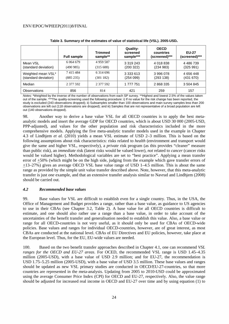
ENV/EPOC/WPIEEP(2011)8/FINAL
24
Table 3. Summary of the estimates of value of statistical life (VSL). 2005-USD.
Full sample Trimmed sample**
Quality- screened sample***
OECD countries
(screened)*** EU-27
(screened)***
Mean VSL (standard deviation)
6 064 679 (490 985)
4 959 587 (315 688)
3 319 243 (200 322)
4 018 838 (234 983)
4 486 739 (325 991)
Weighted mean VSL* (standard deviation)
7 415 484 (885 235)
6 314 696 (301 182)
3 333 613 (254 099)
3 996 078 (293 138)
4 656 448 (431 670)
Median 2 377 592 2 377 592 1 777 751 2 868 335 3 504 845
Observations 856 814 421 259 157 Notes: *Weighted by the inverse of the number of observations from each SP survey. **Highest and lowest 2.5% of the values taken out of the sample. ***The quality-screening used the following procedure: i) If no value for the risk change has been reported, the study is excluded (243 observations dropped); ii) Subsamples smaller than 100 observations and main survey samples less than 200 observations are left out (118 observations are dropped); and iii) Samples that are not representative of a broad population are left out (140 observations dropped).
98. Another way to derive a base value VSL for all OECD countries is to apply the best meta-analytic models and insert the average GDP for OECD countries, which is about USD 30 000 (2005-USD, PPP-adjusted), and values for the other population and risk characteristics included in the more comprehensive models. Applying the five meta-analytic transfer models used in the example in Chapter 4.3 of Lindhjem et al. (2010) yields a mean VSL estimate of USD 2–3 million. This is based on the following assumptions about risk characteristics: risks related to health (environment and transport would give the same and higher VSL, respectively), a private risk program (as this provides “cleaner” measure than public risk), an immediate risk (latent risks would be valued lower), not related to cancer (cancer risks would be valued higher). Methodological variables are set to “best practice”. Applying a mean transfer error of +50% (which might be on the high side, judging from the example which gave transfer errors of +13–27%) gives an average OECD VSL base value range of USD 1–4.5 million. This is about the same range as provided by the simple unit value transfer described above. Note, however, that this meta-analytic transfer is just one example, and that an extensive transfer analysis similar to Navrud and Lindhjem (2008) should be carried out.
4.2 Recommended base values
99. Base values for VSL are difficult to establish even for a single country. Thus, in the USA, the Office of Management and Budget provides a range, rather than a base value, as guidance to US agencies to use in their CBAs (see Chapter 3.2, Table 2). A base value for all OECD countries is difficult to estimate, and one should also rather use a range than a base value, in order to take account of the uncertainties of the benefit transfer and generalisation needed to establish this value. Also, a base value or range for all OECD-countries is not very useful, as it should only be used for CBAs of OECD-wide policies. Base values and ranges for individual OECD-countries, however, are of great interest, as most CBAs are conducted at the national level. CBAs of EU Directives and EU policies, however, take place at the European level. Thus, for the EU, EU-wide values are needed.
100. Based on the two benefit transfer approaches described in Chapter 4.1, one can recommend VSL ranges for the OECD and EU-27 areas. For OCED, the recommended VSL range is USD 1.45–4.35 million (2005-USD), with a base value of USD 2.9 million; and for EU-27, the recommendation is USD 1.75–5.25 million (2005-USD), with a base value of USD 3.5 million. These base values and ranges should be updated as new VSL primary studies are conducted in OECD/EU-27-countries, so that more countries are represented in the meta-analysis. Updating from 2005 to 2010-USD could be approximated using the average Consumer Price Index (CPI) for OECD and EU-27, respectively. Also, the value range should be adjusted for increased real income in OECD and EU-27 over time and by using equation (1) to

ENV/EPOC/WPIEEP(2011)8/FINAL
25
calculate the percentage change in mean GDP per capita in OCED/EU-27 to the power of the income elasticities of VSL suggested below.
101. To derive VSL base value ranges for individual countries within the OCED and EU-27, a unit value transfer with income adjustment (in terms of GDP per capita) of VSL from a study site with population characteristics as similar as possible to the policy site (we transfer to) should be undertaken, using equation (1), reproduced below.
VSLp' = VSLs (Yp / Ys)ß (1)
102. For the income elasticity of VSL, β equal to 0.7- 0.9 (found by Lindhjem et al., 2011, in most of the quality-screened models) is recommended.16 For income Yp and Ys at the policy site and the study sites, respectively; the most current GDP per capita numbers (PPP adjusted, preferably by AIC17
http://stats.oecd.org/Index.aspx
) should be used. This will yield VSLp' in 2005-USD, which should then be converted to national currencies using PPP-adjusted exchange rates for 2005 (see e.g. for GDP numbers and PPP-corrected exchange rates). To adjust VSL to 2010-prices in individual countries, the domestic Consumer Price Index should be used. To correct for increased real income in the same period, VSL should be adjusted with the percentage increase in GDP per capita (in real terms/constant prices), to the power of the income elasticities cited above. If national VSL estimates for a specific policy analysis is needed, one should rather use the 8-step procedure for benefit transfer, conduct unit value transfer from a study with risk and population characteristics as similar as possible to the policy site, add the uncertainty bounds, and then use the meta-analysis to calculate and validate the value range for VSL needed in the specific policy context. This would be the best way to adjust the base value for the factors discussed in Chapter 5.
5. Adjustments to base values – review and recommendations
5.1 Introduction
103. When should a VSL base value be used and when should we try to adjust that base value to improve the accuracy of the VSL estimate? This section addresses this important question of how the transfer of a VSL base value to another policy context should take account of differences in population and risk characteristics and other differences which could potentially determine the appropriate VSL estimate to use.
104. In her comprehensive review of RP and SP studies, Robinson (2008) provides a summary of the empirical evidence for adjustments of the VSL base value for population and risk characteristics, and the implications for Homeland Security regulatory analysis of measures to prevent terrorism attacks. This summary is reproduced in Table 4.
105. Robison (2008) argues that recent wage-risk studies (particularly Viscusi, 2004) provide the most appropriate source for VSL estimates for application in the homeland security context, as terrorists are most likely to target major urban areas with high concentrations of workers. Thus the averted mortality 16 For transfer of VSL from high-income to low-income countries, Hammitt and Robinson (2010) show that
income elasticities larger than 1 should be used. However, transfers between OECD-countries or between EU 27 countries, could apply the elasticities (below 1) found in our meta-analysis of studies from these countries. Transfers from developed to developing countries (outside the dataset in Lindhjem et al. (2010, 2011)) should, however, use income elasticities larger than 1.
17 While GDP per inhabitant is often used as an indicator of countries’ level of economic welfare, it is not necessarily a suitable indicator for households’ actual standard of living. For the latter purpose, a better indicator may be actual individual consumption (AIC) per inhabitant; for further explanations, see: http://epp.eurostat.ec.europa.eu/statistics_explained/index.php/GDP_per_capita,_consumption_per_capita_and_comparative_price_levels.
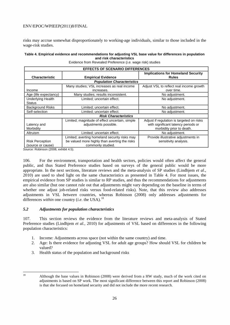
ENV/EPOC/WPIEEP(2011)8/FINAL
26
risks may accrue somewhat disproportionately to working-age individuals, similar to those included in the wage-risk studies.
Table 4. Empirical evidence and recommendations for adjusting VSL base value for differences in population and risk characteristics
Evidence from Revealed Preference (i.e. wage risk) studies
EFFECTS OF SCENARIO DIFFERENCES
Characteristic Empirical Evidence Implications for Homeland Security
Rules Population Characteristics
Income Many studies; VSL increases as real income
increases. Adjust VSL to reflect real income growth
over time. Age (life expectancy) Many studies; results inconsistent. No adjustment. Underlying Health Status
Limited; uncertain effect. No adjustment.
Background Risks Limited; uncertain effect. No adjustment. Self-selection Limited; uncertain effect. No adjustment.
Risk Characteristics
Latency and Morbidity
Limited; magnitude of effect uncertain, simple adjustments possible.
Adjust if regulation is targeted on risks with significant latency periods or
morbidity prior to death. Altruism Limited; uncertain effect. No adjustment.
Risk Perception (source or cause)
Limited; averting homeland security risks may be valued more highly than averting the risks
commonly studied.
Provide illustrative adjustments in sensitivity analysis.
Source: Robinson (2008, exhibit 4.5).
106. For the environment, transportation and health sectors, policies would often affect the general public, and thus Stated Preference studies based on surveys of the general public would be more appropriate. In the next sections, literature reviews and the meta-analysis of SP studies (Lindhjem et al., 2010) are used to shed light on the same characteristics as presented in Table 4. For most issues, the empirical evidence from SP studies is similar to RP studies, and thus the recommendations for adjustments are also similar (but one cannot rule out that adjustments might vary depending on the baseline in terms of whether one adjust job-related risks versus food-related risks). Note, that this review also addresses adjustments in VSL between countries, whereas Robinson (2008) only addresses adjustments for differences within one country (i.e. the USA).18
5.2 Adjustments for population characteristics
107. This section reviews the evidence from the literature reviews and meta-analysis of Stated Preference studies (Lindhjem et al., 2010) for adjustments of VSL based on differences in the following population characteristics:
1. Income: Adjustments across space (not within the same country) and time. 2. Age: Is there evidence for adjusting VSL for adult age groups? How should VSL for children be
valued? 3. Health status of the population and background risks
18 Although the base values in Robinson (2008) were derived from a HW study, much of the work cited on
adjustments is based on SP work. The most significant difference between this report and Robinson (2008) is that she focused on homeland security and did not include the more recent research.

ENV/EPOC/WPIEEP(2011)8/FINAL
27
Income
108. Empirical evidence as well as the meta-analysis of Lindhjem et al. (2010) show, as expected from economic theory, that people’s WTP increases with income, and thus VSL increases with income. Ethical concerns, however, could prevent the use of different VSL estimates for different income groups within a country. The same is true for a group of countries, like the European Union, when performing CBAs of new EU directives involving changes in mortality risks. Even for global environmental problems, like climate change, one can see increased use of equity-weighting in CBAs in terms of using the same VSL for poor as for rich countries (Tol, 2005; Stern, 2008; and Anthoff et al., 2009). However, for CBAs on the national level, which is the most common level for regulatory analyses, national VSL estimates should be used (to reflect the preferences of the national population). These national VSL estimates could, however, differ with respects to risk characteristics and population characteristics other than income.
109. Viscusi (2010) argues that even if meta-analyses of wage risk studies show an income elasticity of 0.5-0.6, this is just for the restricted age-spectrum covered in wage risk studies, and that it should be around 1.0 for the general public. Lindhjem et al. (2011), however, find an income elasticity of 0.7-0.9 for most of the quality-screened models of SP studies of the general public. Since this meta-analysis is based on studies of the general public, we suggest using an elasticity of 0.8 (i.e. the midpoint of 0.7 and 0.9) in the equation (1) in Chapter 2.1 when conducting a CBA at the national level, and there is a need to transfer a VSL estimate from another country. As a sensitivity analysis, we recommend using 0.4, since Lindhjem et al. (2011) also found this lower elasticity for a subset of studies in the meta-analysis that use the same high-quality survey instruments or satisfied the scope test (i.e. verifying that people are willing to pay significantly more for a larger risk reduction than a smaller one).
Age
110. The reluctance to make age adjustments in the U.S. stems from the significant controversy that erupted over the so-called “senior discount”, where the U.S. EPA used a lower VSL for older individuals in sensitivity analyses conducted for air pollution rules prior to 2004, including the Clear Skies Initiative, where benefits to senior citizens constituted the majority of the policy benefits (Robinson, 2007). Because environmental policies often reduce risks to the very young or the very old, the age differentiation with regards to VSL arose first in this sector. Aldy and Viscusi (2007) note that negative direction of the change in valuation of older people´s lives, rather than recognition of heterogeneity in VSL, may have accounted for the public uproar that the benefit assessment created. If the US EPA had instead placed a premium on the lives of children whose risks would be reduced by the policy, it is likely that few would have objected. Aldy and Viscusi op. cit. also point out that whether VSL should vary by age is not a matter of equity or political expediency, but should rather be grounded on estimates of how people’s WTP for risk reductions vary with age. As we age, our life expectancy shortens, but our economic resources vary as well, giving rise to a theoretical indeterminacy in the age-VSL relationship (see also Viscusi, 2009).
111. While there is some empirical evidence that VSL declines at older age, recent work suggest this relationship is uncertain (Hammitt, 2007; Aldy and Viscusi, 2007; Krupnick, 2007). Thus, determining the VSL at different ages requires more research. Age differentiation in VSL will facilitate better prioritisation of mortality risk reduction efforts for populations of various ages. Two US expert panels have advised against making VSL age adjustments due to inconclusive evidence (Cropper et al., 2007; National Academy of Sciences, 2008).
112. Lindhjem et al. (2010) in their meta-analysis of SP studies of adult VSL find no clear relationship between age and VSL, although for a subset of the data, indications of an inverted U-shape relationship between VSL and mean age of the sample was found (meaning that VSL increase with age to about 40-50 years of age and then decline).

ENV/EPOC/WPIEEP(2011)8/FINAL
28
113. VSL appears to be higher for children, due to parents’ altruistic concerns for their children, with results from the US and Europe indicating VSL for children being as high as a factor of 2 that of their parents/ adults (US EPA, 2003; OECD, 2010). More generally, in cases where the policy intervention particularly affects children, due to the nature/scope of policy (e.g., pesticides in school grounds) or because children are particularly vulnerable to this particular hazard (e.g., lead in drinking water), then child-specific values are likely to be particularly helpful in ensuring that resources and policy efforts are allocated efficiently. According to OECD (2010), it is likely that the introduction of a ‘premium’ for children would raise less controversy than a ‘discount’ for seniors. Since ‘children’ were not included in those studies, which are usually used to determine baseline VSLs, the ‘premium’ could be simply added to the baseline estimate. Moreover, there is a stronger political case. While the interests of children are usually defended by parents (and other caregivers), policy makers in OECD governments have always had a special role in protecting the interests of children with respect to risks in general. In some cases (i.e. negligence or abuse), this role may supersede that of their parents. As such, there is, at least, a distinct obligation with respect to children’s risks to determine whether or not a premium should be applied.
114. Based on literature reviews and the SP meta-analysis no adjustment for age is recommended. However, when the policy analysed targets children specifically (or affects mainly children), a higher VSL for children is recommended. Based on the available empirical evidence from the US and Europe (see Chapter 2.1) VSL for children should be 1.5–2.0 times higher than the mean adult VSL.
Health status of the population and background risks
115. Regarding a relationship between health status and VSL, the SP evidence is very limited and inconclusive. The principal studies that have explored this linkage are Johannesson and Johansson (1996) that found that WTP values declined with poorer health status, while Krupnick et al. (2000) found no significant evidence of such a relationship.
116. Since few SP studies contain information about health status of the population and the background/baseline risks, these variables were not included in the final version of the meta-analysis (Lindhjem et al., 2010). There were some indications that baseline risks may affect VSL in some earlier regressions, but theoretically the baseline risk is not expected to affect WTP and VSL very much, at least not for small levels of risks.
117. Based on the literature review and the SP meta-analysis no adjustment for health status of the population and background risks is recommended.
5.3 Adjustments for risk characteristics
118. This section reviews the evidence from the literature reviews and the meta-analysis of Stated Preference studies (Lindhjem et al., 2010) for adjustments of VSL based on differences in the following risk characteristics:
Timing of risks (Latency)
119. As expected from theory, there is empirical evidence that people value mortality risk where there is a time lag between the measure and the impact lower than immediate mortality risk reductions. Lindhjem et al., (2011) provide mixed evidence for latency, but studies using the same high-quality survey instrument or pass both internal and external scope tests (i.e. people have higher WTP for larger risk reductions) show latent risk reductions to lead to lower VSL estimates.

ENV/EPOC/WPIEEP(2011)8/FINAL
29
120. Based on the literature review and the SP meta-analysis, no adjustments should be made for latency in base VSL values. However, if the regulation is targeted on risks with significant latency periods; a sensitivity analysis adjusting VSL downwards should be performed, using Lindhjem et al. (2011, table VII, model 1).
Risk perception (source or cause)
121. Some research suggest that risks that are viewed as less controllable, voluntary and familiar may be valued up to twice as high as other risks (Robinson et al., 2010). Jones Lee and Loomes (1995) compare events that differ in magnitude, but found little evidence of a scale premium. They suggest that, in the case of rare catastrophic events, aversion to ambiguity may be counterbalanced by doubts about whether programmes can be designed to effectively avert such risks.
122. Lindhjem et al. (2011) finds that while in the full, unscreened dataset transport related mortality risks are valued higher than health and environmental risks, in the quality-screened models, VSL estimated from SP surveys explicitly mentioning that the mortality risk is environmentally related is valued lower than health and transport sector studies. However, as the types of risks valued within these categories seem heterogeneous, one should be cautious in interpreting these results.
123. Based on the literature review and the SP meta-analysis, VSL should not be adjusted for whether the regulatory analysis considers measures in the health, environment or transport sectors. However, sensitivity analysis for lower values in the transport and environment sectors than health should be carried out.
Cancer / Dread (Morbidity prior to death)
124. WTP to reduce the risk of cancer death may be greater than for accidental death, e.g. because of the lengthy and painful illness and treatment process that frequently precedes death from cancer. Chestnut and De Civita (2009) in their literature review points to studies indicating that this effect exists. However, they conclude that the available valuation research is not sufficient at this time to determine the direction and the magnitude of applying available VSL estimates to cancer death. On-going Stated Preferences studies in EU-projects, like EXIOPOL and HEIMTSA, will shed more light on this adjustment factor.
125. Lindhjem et al. (2010) find a cancer premium in the meta-analysis of the full, unscreened dataset, but not in the quality-screened models.
126. The literature review and the meta-regressions of Lindhjem et al. (2011) do not support adjusting VSL upwards if the regulation is targeting cancer risks. Thus, we recommend not adjusting VSL for cancer risks, but account for the costs of morbidity prior to cancer deaths separately.
5.4 Adjustments of VSL in space and time
127. VSL estimates vary in space (i.e. between countries) and over time. For transfer between countries, Purchasing Power Parity (PPP) adjusted exchange rates should be used to also correct for how differences in the costs of living affect VSL (which is not reflected in the market exchange rates for different currencies).
128. To update VSL estimates over time, the same VSL study repeated over time is needed to establish a price index for VSL. In lack of this empirical evidence and a specific price index for VSL, the Consumer Price Index (CPI) is frequently used to update VSL estimates over time. This practice assumes that how people value mortality risks over time follows the same pattern as their willingness-to-pay for the

ENV/EPOC/WPIEEP(2011)8/FINAL
30
basket of consumer goods the CPI is based on. A research programme repeating the same best practise stated preference study of mortality risk for many years in several countries would provide more reliable estimates for how the general population value mortality risks in space and time.
129. Even if the income elasticity of VSL is not used to adjust VSL for income differences within a country, it is frequently used to adjust VSL over time to take account of an increase in income (often in terms of GDP per capita) in real terms (not nominal) over time.
130. As we lack empirical evidence on how VSL estimates develop over time, the Consumer Price Index of the policy country is recommended for conversion of VSL to the current price level. An income elasticity of 0.8 is recommended for adjusting VSL for changes in real income over time within the OECD and EU-27 countries; which means that 1% increase in real GDP per capita will result in a 0.8% increase in VSL. A sensitivity analysis using an income elasticity of 0.4 should be performed (as some of the quality-screened models of Lindhjem et al. (2011) show this lower income elasticity).
“Discount factor” for hypothetical bias in Stated Preference studies?
131. Compared to meta-analysis of wage risk studies, the meta-analysis of stated preference (SP) studies (mostly Contingent Valuation studies) by Braathen et al., 2009 / Lindhjem et al., 2010 provides “conservative”, lower estimates. The issue of hypothetical bias in SP studies is still a concern, but there is no general agreement of a “discount factor” to account for this potential difference in stated and “true” willingness-to-pay. SP studies have the great advantage over wage risk studies in that they can reflect preferences of the general population for different risk contexts rather than just job related risks for workers in a restricted age group (excluding children and the older adults).
Adding other social costs of the fatality
132. Average private and public costs of dealing with a fatality (treatment, hospital, etc.) should be added to the VSL to estimate the total social value of preventing a fatality. One should, however, be aware of the possible double counting of morbidity and mortality effects when summing of all health effects in a CBA. Also, there are no widely-accepted standards for estimating these costs, and different studies might results in significantly different estimates (see e.g. Akobundu et al., 2006; Blom et al., 2001; and Yabroff et al., 2009). Since these costs are generally very small relative to VSL, ignoring these costs may not noticeably affect the analytic results.
Altruism and private vs. public risks
133. Private valuation of private risk is the most common scenario in both wage risk and SP studies. Thus, altruistic concerns need to be added for policies affected public mortality risk like e.g. air pollution policies. According to Strand (2004);
“whenever paternalistic altruism dominates (respondents attach “considerably more” weight to other persons’ survival probabilities than to their general consumption), it may be legitimate to include altruistically expressed values as part of “true” VSL. Elicitation of VSL as a purely private good may then be misleading in public policy contexts where mortality risk reductions almost always are of the public good kind”.
134. Strand (2003) argues that the altruism expressed by adults for their children does not cease to exist once children are older than 18 and are asked to value risk in SP studies. Despite lower income for young adults, their VSL is much higher due to the fact that many people have altruistic values for them. Older people typically have higher income themselves (and higher WTP for risk), but the altruistic values from others may be less strong than for young adults.

ENV/EPOC/WPIEEP(2011)8/FINAL
31
135. However, no general adjustment factor for altruism for studies valuing private risk can be found in the literature. On the contrary, several SP studies find significantly lower WTP for public risks than for private risks (Svennson and Vredin Johansson, 2007), and so does the meta-analysis of SP studies of Lindhjem et al. (2010, 2011). Svennson and Vredin Johansson op.cit., find, based on the results from a purpose-made survey, that part of the discrepancy can be explained by the individuals’ age and his/her attitudes towards privately and publicly provided goods in general. Due to differences in attitudes, they argue that public and private goods are in fact perceived as a two different goods, even if the risk reductions are of equal magnitudes. However, one cannot fully exclude that methodological issues of the SP method might have influenced their results. Thus, the difference in valuation when the risk change affects the individual or her household members versus the public at large is still unexplained. Altruism would pull in the direction of higher WTP and VSL for public risk changes. On the other hand, private risk changes are typically something the family or individual controls through buying a helmet or a product that reduces risk. In other words, the risk change is more concrete and direct when it is private compared to a public risk program. Thus, one can argue that SP studies of private risks provides “cleaner” estimates of VSL, and should be the main basis of VSL estimates until this difference can be fully explained.
6. Conclusions and recommendations
136. Regulatory practises with regards to how to establish the Value of a Statistical Life (VSL) varies widely between countries, and even between agencies within a country. The main difference between the US and Europe is the reliance of Revealed Preference (RP) methods in terms of wage risk studies in the US (where most such studies have been conducted), while Europe relies on Stated Preference methods, eliciting people’s willingness-to-pay (WTP) for changes in mortality risks. Two other countries in the forefront of mortality valuation, Canada and Australia, also increasingly rely on SP studies.
137. VSL from a SP survey can be derived in the following way: A SP survey finds an average WTP of $30 for a reduction in the annual risk of dying from air pollution from 3 in 100,000 to 2 in 100,000. This means that each individual is willing to pay $30 to have this 1 in 100,000 reduction in risk. In this example, for every 100,000 people, one death would be prevented with this risk reduction. Summing the individual WTP values of $30 over 100,000 people gives the number referred to as value of statistical life (VSL). The VSL estimate in this case is $3 million. It is the aggregate WTP for the group in which one death would be prevented. It is important to emphasize that the VSL is not the value of an identified person’s life, but rather an aggregation of individual values for small changes in risk of death.
138. The VSL is often used in cost-benefit analysis (CBA) of policies as follows. The analyst first estimates the number of deaths expected to be prevented in a given year by multiplying the annual average risk reduction by the number of people affected by the program. Then the VSL (either a single number or a range) is applied to each death prevented in that year in order to estimate the annual benefit. Annual benefits are then summed over the life time of the policy as a present value using the national social discount rate.
139. An 8-step procedure for transferring VSL estimates from existing SP studies for use in a regulatory policy analysis /CBA is outlined. A simple unit value transfer with income adjustment in terms of GDP per capita, using equation (1) (reproduced below), is recommended when transferring VSL estimates from other countries to establish a domestic VSL base value.
VSLp' = VSLs (Yp / Ys)ß (1)
140. For the income elasticity of VSL, β equal to 0.8 (found by Lindhjem et al., 2011, in most of the quality-screened models) is recommended. Since some of the quality screened models showed lower income elasticities, a sensitivity analysis of β equal to 0.4 should be performed. For income Yp and Ys at

ENV/EPOC/WPIEEP(2011)8/FINAL
32
the policy site and the study sites, respectively; the most current GDP per capita numbers (PPP adjusted, preferably by AIC) should be used. This will yield VSLp' in 2005-USD, which should then be converted to national currencies using PPP-adjusted exchange rates for 2005 (see e.g. http://stats.oecd.org/Index.aspx for GDP numbers and PPP-corrected exchange rates). To adjust VSL to 2010-prices in individual countries, the domestic Consumer Price Index should be used. To correct for increased real income in the same period, VSL should be adjusted with the percentage increase in GDP per capita (in real terms/constant prices) to the power of the income elasticities cited above
141. The OECD database for SP studies of VSL19
142. Literature reviews and the most comprehensive meta-analysis of stated preference (SP) studies worldwide (Lindhjem et al., 2010, 2011) are used to establish a base range for the average VSL for OECD countries of USD 1.45–4.35 million (2005-USD), with a base value of USD 2.9 million. For EU-27, the corresponding base range is USD 1.75–5.25 million (2005-USD), with a base value of USD 3.5 million. Table 5 summarizes the recommendation for when the base value range for a country (or group of countries) should be adjusted or not.
should be used to identify SP studies that are as similar as possible with respect to the population and risk characteristics listed in Table 4. An uncertainty (transfer error) of + 20-100% should be added to the VSL base value dependent on the similarity between the study transferred from (termed study context) and the policy analyzed (termed policy context). The quality-adjusted/screened meta-analysis results should be used to increase the validity of the unit transfer. When there is no similar study to transfer VSL estimates from, meta-analysis is the only possibility, but then a transfer error of +100% should be added according to the 8-step guidelines. However, the empirical evidence from the meta-analysis of SP studies (Lindhjem et al., 2010, 2011) shows that adding an error bound of +50% to the calculated mean value would cover the uncertainty of the transfer.
Table 5. Recommendations for adjusting VSL base values Based on Stated Preference studies for differences in population and risk characteristics and other differences.
Adjustment factor Recommendation Population Characteristics
Income
No adjustment within a country or group of countries the policy analysis is conducted for (due to equity concerns). For transfers between countries VSL should be adjusted with the difference in
Gross Domestic Product (GDP) per capita to the power of an income elasticity of VSL of 0.8, with a sensitivity analysis using 0.4 (see
equation (1) in chapter 2.1.)
Age
No adjustment for adults due to inconclusive evidence. Adjust if regulation is targeted on reducing children´s risk. VSL for children
should be a factor of 1.5 – 2.0 higher than adult VSL. Health Status of population and
background risk No adjustment (due to limited evidence) Risk Characteristics
Timing of risk (Latency)
No adjustment. As a sensitivity analysis, adjust downwards using Lindhjem et al. (2011, table VII model 1) if the regulation is targeted
on risks with significant latency periods.
Risk Perception (source or cause) No adjustment (due to inconclusive evidence). Sensitivity analysis for
lower values in the environment sector than in health and traffic.
Cancer or Dread (Morbidity prior to death)
No adjustment if regulation is targeted on cancer risks and/or risks that are dreaded due to morbidity prior to death. Morbidity costs prior
to death should be added separately.
Magnitude of risk change
No adjustment. However, since the magnitude of the risk change clearly affects the VSL, a sensitivity analysis based on VSL calculated
from a risk change similar in magnitude to the policy context should be conducted. A risk change of 1 in 10,000 annually is suggested for
19 See www.oecd.org/env/policies/vsl.

ENV/EPOC/WPIEEP(2011)8/FINAL
33
calculating a VSL base value. Other adjustments
Altruism and Public vs. Private risk
No adjustment (due to limited evidence and unresolved issues). Use “Private risk” to calculate a VSL base value. Provide illustrative
adjustments in sensitivity analysis. Discount for hypothetical bias in SP
studies No adjustment (due to limited evidence) Correction for inflation Adjustment based on the national Consumer Price Index (CPI)
Correction for increased real income over time
Adjust VSL with same percentage as the percentage increase in GDP per capita
143. Robinson and Hammitt (2010) recommend extending the US EPA approach of extensive use of independent experts to revision of VSL estimates across all US regulatory agencies in order to get more comparable analytical results and allow decision makers to understand why different VSL estimates are used, and avoid duplications in efforts across agencies. The US EPA approach involves funding new primary research, periodically evaluating the available evidence, and submitting recommendations to its Science Advisory Board for review. This approach to co-ordination and continuous revision of VSL base ranges and values and adjustments should be extended also outside the US to EU-27 and all OECD-countries, and include continuous updating of the OECD data base and meta analysis for SP surveys (Lindhjem et al., 2010, 2011).

ENV/EPOC/WPIEEP(2011)8/FINAL
34
ANNEX: EXAMPLES OF VSL APPLICATIONS
144. An example of how to use VSL in different contexts is presented below; for use in a workshop with policy-makers.
145. In its guidelines for the estimation of the benefits of environmental policies (US EPA, 2000), the US Environmental Protection Agency recommends using a VSL of USD 6.1 million (1999 dollars). To arrive at this figure, the Agency compiled VSL values from 26 studies, mostly compensating wage studies. The US EPA does not adjust the VSL for age, futurity of the risk, and cancer, but it does adjust it for growth in income.
146. The European Commission used a working group set up by EC DG ENV (2000) to debate valuation of mortality end-points and define “interim” values. The Working Group’s firm preference was for estimates based on the VSL, given the absence of direct empirical estimates of VOLYs. The working group considered evidence on the VSL from wage-risk studies and contingent valuation studies, and considered the latter to be the more robust for defining society’s willingness to pay to reduce risk. The group agreed on an upper limit defined by the VSL identified in the ExternE research (www.externe.info) – EUR 4.1 million in 2005 prices. The group was, however, persuaded that recent methodological advances in non-market valuation should be taken into account in establishing a VSL for DG ENV use. On this basis, the value of EUR 1.5 million (2005 prices) was identified as a baseline figure. This provided a best estimate of EUR 1.1 million for the VSL after adjusting down to account for the age of those likely to be affected using a factor of 0.7. A lower estimate of EUR 0.75 million was based on research by Krupnick et al. (2002) in North America. A number of other adjustments relating to potential air pollution-specific valuation issues were considered, but not adopted. Table A.1 presents a summary of adjustments made by DG ENV.
Table A.1: EC Policy guidance on unit values in 2000 (2005 prices)
Adjustment factor EC Guideline Baseline VSL Central: €1.5m; Range: €0.75 - €3.75m Context 50% premium for cancer Age Multiplier of 0.7 (applies to central value only) Health No adjustment Cultural No adjustment Income No adjustment Final Unit Values Central: €1.1m; Range: €0.75 - €3.75m Futurity Discount rate: 4%
147. Subsequently, however, the European Commission funded a new empirical study of mortality risk valuation. This study, reported in Markandya et al. (2004), later published as Alberini et al. (2006), had as its objective the derivation of unit values to account in monetary terms for the incidence of premature death estimated to result from air pollution in Europe. Values were derived from three surveys undertaken simultaneously in UK, France and Italy, using a common survey instrument previously developed in North America (Krupnick et al., 2002).
148. The Clean Air for Europe (CAFE) CBA, undertaken by DG Environment as part of the Air Quality Thematic Strategy, on behalf of the European Commission, (Watkiss et al., 2005), applied the results of Markandya et al. (2004). Emphasis was given to the results of this study over the study

ENV/EPOC/WPIEEP(2011)8/FINAL
35
undertaken in the UK by DEFRA that valued extensions in life expectancy (and so, VOLY) directly (Chilton et al., 2004). This preference was a) on the basis that Markandya et al. was more representative of the EU population, covering three EU Member States compared to one, and b) that it had a much larger sample size. On the basis of Rabl (2002), the study derived the changes in remaining life expectancy, and therefore the corresponding VOLY, associated with the 5 in 1,000 risk change over the next 10 years (i.e. an annual risk reduction of 5 in 10,000) using empirical life-tables. Thus, both VSL and VOLY could be used in the health impact assessment.
149. The CAFE CBA considered an adjustment for the quality of the life lost. The Markandya et al. study found that the fact that a respondent has a chronic heart or lung condition does not influence WTP per se. However, those persons who have been hospitalized for cardiovascular or respiratory illnesses over the last 5 years had WTP amounts that were, everything else being the same, roughly twice as large as those of all others. Therefore, as a sensitivity test, a multiplier of two was applied. The WTP was not found to be age-dependent, so no adjustment was made for age.
Table A2. Values for use in CAFE CBA: Effects of chronic exposure on mortality. (EUR, 2005 prices)
VSL VOLY Derived from: Median (NewExt) 1 109 000 59 200 Median WTP for an annual risk reduction of 5:10,000 Mean (NewExt) 2 280 000 143 000 Mean WTP for an annual risk reduction of 5:10,000 Source: Watkiss et al. (2005).

ENV/EPOC/WPIEEP(2011)8/FINAL
36
REFERENCES
Akobundu, E., J. Ju, L. Blatt and C.D. Mullins. (2006), “Cost-of-Illness Studies: A Review of Current Methods”, Pharmacoeconomics. 24(9), 869-890.
Alberini, A., et al. (2004), “Does the Value of a Statistical Life Vary with Age and Health Status? Evidence from the US and Canada”. Journal of Environmental Economics and Management, no. 48: 769-792.
Alberini, A., A. Hunt, and A. Markandya (2006), “Willingness to Pay to Reduce Mortality Risks: Evidence from a Three-Country Contingent Valuation Study”. Environmental and Resource Economics, 33, no. 2: 251-264.
Aldy, J. and W. Kip Viscusi (2007), “Age Differences in the Value of Statistical Life: Revealed Preference Evidence”, in Review of Environmental Economics and Policy 2007 1(2):241-260.
Anthoff , D., C. Hepburn and R.S.J. Tol (2009): Equity weighting and the marginal damage costs of climate change. Ecological Economics 68; 836-849.
Australian Government (2008), The health of nations: The value of a statistical life. July 2008.
Australian Government (2008), Best Practice Regulation Guidance Note: Value of statistical life. Office of Best Practice Regulation, Department of Finance and Deregulation.
Baker, R., S. Chilton, M. Jones-Lee, and H. Metcalf. (2008), “Valuing Lives Equally: Defensible Premise or Unwarranted Compromise?” Journal of Risk and Uncertainty. 36, 125–138.
Bateman, I., et al. (2009), Valuing Environmental Impacts: Practical Guidelines for the Use of Value Transfer in Policy and Project Appraisal. Value Transfer Guidelines. Eftec, London. Submitted to Department for Environment, Food and Rural Affairs (Defra), Dec. 2009. www.defra.gov.uk/environment/policy/natural-environ/using/valuation/index.htm.
Biausque, V. (2010), The Value of Statistical Life: A Meta-Analysis, OECD, Paris. See www.oecd.org/env/policies/vsl.
Blomquist, G. (2004), “Self-Protection and Averting Behaviour, Values of Statistical Lives, and Benefit-Cost Analysis of Environmental Policy”. Review of Economics of the Household 2; 89-110.
Bloom, B.S., D.J. Bruno, D.Y. Maman and R. Jayadevappa. (2001), “Usefulness of U.S. Cost of Illness Studies in Healthcare Decision Making”, Pharmacoeconomics. 19(2), pp. 207-213.
Braathen, N. A, H. Lindhjem and S. Navrud (2009), Valuing Lives Saved from Environmental, Transport and Health Policies: A Meta-analysis of Stated Preference Studies. OECD, Paris. See www.oecd.org/env/policies/vsl.
Cameron, T.A. (2010), “Euthanizing the Value of a Statistical Life.” Review of Environmental Economics and Policy. 4(2), 161-178.
ENV/EPOC/WPIEEP(2011)8/FINAL
37
Chestnut, L. G. And P. De Civita (2009), Economic valuation of mortality risk reduction: Review and recommendations for policy and regulatory analysis. Research paper. Government of Canada.
Chilton, S., et al. (2004), Valuation of Health Benefits Associated with Reductions in Air Pollution: Final Report, Defra. London.
Cropper, M. et al. (2007), SAB Advisory on EPA’s “Issues in Valuing Mortality Risk Reduction”. Memorandum from the Chair, Science Advisory Board, and the Chair, Environmental Economics Advisory Committee, to EPA Administrator Stephen L. Johnson. EPA-SAB-08-001.
Desaigues, B. et al. (2011), “Economic valuation of air pollutants”, Ecological Indicators 11 (3); 902 – 910.
European Commission DG Environment (2001), Recommended interim values for the value of preventing a fatality in DG Environment cost benefit analysis. See http://ec.europa.eu/environment/enveco/others/pdf/recommended_interim_values.pdf.
European Commission (2009), Impact Assessment Guidelines, SEC(2009) 92.
Hammitt, J.K. (2007), “Valuing changes in mortality risk: Lives saved versus life years saved”, Review of Environmental Economics and Policy, 1(2), 228-240.
Hammitt, J.K. and L. Robinson (2010): “The Income Elasticity of the Value per Statistical Life: Transferring Estimates Between High and Low Income Populations”, Journal of Cost Benefit Analysis. Manuscript 1009. Berkeley Electronic Press.
IGCB (2007), An Economic Analysis to inform the Air Quality Strategy. Updated third report of the Interdepartmental Group on Costs and Benefits (IGCB). Volume 3. Annex 2 – Valuing the health benefits associated with reductions in air pollution – recommendations for valuation. Department of Environmental, Food and Rural affairs (Defra). July 2007.
Johannesson, M., and P-O. Johansson (1996), “To Be, or Not to Be, That Is the Question: An Empirical Study of the WTP for an Increased Life Expectancy at an Advanced Age”, Journal of Risk and Uncertainty, 13, 163-174.
Jones-Lee, M.W. and G. Loomes (1995), “Scale and Context Effects in the Valuation of Transport Safety”,Journal of Risk and Uncertainty, 11(3); 183-203.
Kochi, I. et al. (2006), “An Empirical Bayes Approach to Combining and Comparing Estimates of the Value of a Statistical Life for Environmental Policy Analysis”, Environmental and Resource Economics. 34, 385-406.
Krupnick, A. (2007), “Mortality-risk valuation and age: Stated preference evidence”, Review of Environmental Economics and Policy, 1 (2), 261-282.
Krupnick A. et al. (2000), What Are Older People Willing to Pay to Reduce Their Risk of Dying?, Resources For the Future, Washington DC.
Krupnick, A. et al. (2002), “Age, Health and the Willingness to Pay for Mortality Risk Reductions: A Contingent Valuation Survey of Ontario Residents”, Journal of Risk and Uncertainty, 24 (2), pp. 161-186.

ENV/EPOC/WPIEEP(2011)8/FINAL
38
Kristofersson , D. and S. Navrud (2007), “Can Use and Non-Use Values be Transferred Across Countries?”. In: S. Navrud and R. Ready (2007) (ed.), Environmental Value Transfer: Issues and Methods, Springer, Dordrecht, The Netherlands.
Lindhjem, H. et al. (2010), Meta-analysis of stated preference VSL studies: Further model sensitivity and benefit transfer issues. OECD, Paris. See www.oecd.org/env/policies/vsl.
Lindhjem, H. et al. (2011), “Valuing mortality risk reductions from environmental, transport and health policies: A global meta-analysis of stated preference studies”. Submitted to Risk Analysis.
Lindhjem, H. and S. Navrud (2008), “How Reliable are Meta-Analyses for International Benefit Transfer?”, Ecological Economics, 66(2-3); 425-435.
Markandya, A., et al. (2004), EC NewExt Research Project: Mortality Risk Valuation, Final Report, European Commission, Brussels.
Mrozek J R and Taylor L O (2002), “What determines the value of life? A Meta-analysis”. Journal of Policy Analysis and Management, 21(2): 253-270
National Academy of Sciences (2008), Estimating Mortality Risk Reduction and Economic Benefits from Controlling Ozone Air Pollution. Committee on Estimating Mortality Risk Reduction Benefits from Decreasing Tropospheric Ozone Exposure. Washington D.C.: National Academies Press.
Navrud, S. (2004), “Value transfer and environmental policy”, in Tietenberg, T. and H. Folmer (eds.) (2004), The International Yearbook of Environmental and Resource Economics 2004/2005. A survey of Current Issues. Edward Elgar Publishing, Cheltenham, UK and Northampton, MA, USA.
Navrud, S. (2007), Practical tools for value transfer in Denmark – guidelines and an example. Working Report No. 28, 2007, Miljøstyrelsen (Danish Environmental Protection Agency), Copenhagen http://www2.mst.dk/common/Udgivramme/Frame.asp?pg=http://www2.mst.dk/Udgiv/publications/2007/978-87-7052-656-2/html/kap06_eng.htm.
Norwegian Directorate for Public Roads (2006), Impact Analysis (In Norwegian; “Konsekvensanalyser”). Handbook 140. Directorate for Public Roads, Oslo.
Norwegian Ministry of Finance (2005), A Guide to Economic Regulatory Analysis (In Norwegian; ”En veileder til Samfunnsøkonomiske Analyser”). Norwegian Ministry of Finance, Oslo, Norway. www.regjeringen.no/upload/kilde/fin/reg/2005/0029/ddd/pdfv/266324-veileder_i_samfunnsok_analyse_trykket.pdf.
OECD (2010), Valuing Environment-Related Health Impacts - with special emphasis on children (VERHI-Children). Final report. OECD, Paris.
Rabl, Ari (2002), Relation Between Life Expectancy and Probability of Dying. Report Centre d’Energétique, Ecole des Mines, 60 boul. St.-Michel, F-75272 Paris.
Ready, R.C. et al. (2004), “Benefit Transfer in Europe. How Reliable Are Transfers Between Countries?” Environmental and Resource Economics 29; 67-82.
Robinson, L.A. (2007), “How U.S: government agencies value mortality risk reductions”. Review of Environmental Economics and Policy, 1 (2); 289-299.

ENV/EPOC/WPIEEP(2011)8/FINAL
39
Robinson, L. (2008), Valuing mortality risk reductions in homeland security regulatory analyses. Final report. June 2008. Available from http://regulatory-analysis.com/pub.htm.
Robinson, L. A. and J. K. Hammitt (2010), “Valuing health and longevity in regulatory analysis: Current issues and challenges”. Jerusalem papers in regulation & governance. Working paper No 4.
Robinson, L. A. et al. (2010), “Valuing the Risk of Death from Terrorist Attacks”, Journal of Homeland Security and Emergency Management 7(1), Article 14; 1-25.
Scotton, C. R. and L. O. Taylor (2010), “Valuing risk reductions: Incorporating risk heterogeneity into a revealed preference framework”, Resource and Energy Economics, Vol. 33, pp. 381-397
Smith, V.K. et al. (2006), “Structural Benefit Transfer: An Application Using VSL Estimates”, Ecological Economics. 60, 361-371.
Söderqvist, T. and Å. Soutukorva (2006), An instrument for assessing the quality of environmental valuation studies. Report. Swedish Environmental Protection Agency (Naturvårdsverket) www.naturvardsverket.se/bokhandeln/pdf/620-1252-5.pdf.
Stern, N. (2005), “The economics of climate change”. Richard T. Ely Lecture, American Economic Review: Papers & Proceedings 2008, 98; 2–37.
Strand, J. (2003), Interpersonal factors in the valuation of statistical lives. Department of Economics, University of Oslo, Norway, august 2003. http://folk.uio.no/jostrand/interpersonalpaper.pdf.
Strand, J. (2004), Public- and private-good values of statistical lives: Results from a combined choice-experiment and contingent-valuation survey. May 2004. Department of Economics, University of Oslo, Norway, http://folk.uio.no/jostrand/lifepaper02.pdf.
Svensson M. and M. Vredin-Johansson (2010), “Willingness to Pay for Private and Public Safety: Why the Difference?” Accident Analysis & Prevention, 42: 1205-1212.Tol, R. S. J. (2005), “The marginal costs of carbon dioxide emissions: An assessment of the uncertainties”, Energy Policy 33; 2064-2074.
Treasury Board of Canada, Secretariat (2007), Canadian Cost-Benefit Analysis Guide: Regulatory Proposals (Interim).
US EPA (2000), Guidelines for preparing economic analyses.Washington D.C., US. EPA http://yosemite.epa.gov/EE/epa/eed.nsf/Webpages/Guidelines.html.
US EPA (2003), Children‘s Health Valuation Handbook. Washington D.C., US. EPA http://yosemite1.epa.gov/ee/epa/eed.nsf/3cdbd09d7c867d9785256c9200548b12/6ed3736d44c87a4a85256dc1004da4ac/$FILE/handbook1030.pdf .
US EPA (2006), Report of the EPA Work Group on VSL Meta-Analysis, Report NCEE-0494, National Center for Environmental Economics, US EPA. http://yosemite.epa.gov/ee/epa/eerm.nsf/vwRepNumLookup/EE-0494?OpenDocument.
US EPA (2008), Guidelines for preparing economic analyses. External review draft. US EPA http://yosemite.epa.gov/EE/epa/eerm.nsf/vwRepNumLookup/EE-0516?OpenDocument.

ENV/EPOC/WPIEEP(2011)8/FINAL
40
UK DfT (2009), Guidance Document – Expert. TAG unit 3.4.1: The Accidents Sub-Objective. UK Department of Transport (DfT), London, July 2009 . www.dft.gov.uk/webtag/documents/expert/unit3.4.php#2_2.
Viscusi, W.K. (2004), “The Value of Life: Estimates with Risks by Occupation and Industry”, Economic Inquiry. Vol. 42, No. 1, pp. 29-48.
Viscusi, W.K. (2009), “The devaluation of life”, Regulation & Governance 3; 103-127.
Viscusi, W.K. (2010), “The heterogeneity of the value of statistical life: Introduction and overview”, Journal of Risk and Uncertainty 40(1); 1-13.
Viscusi, W.K. and J.E. Aldy (2003), “The Value of a Statistical Life: A Critical Review of Market Estimates throughout the World”, Journal of Risk and Uncertainty, 27(1), p. 5-76.
Viscusi, W. Kip and Joseph E. Aldy (2007), “Labor Market Estimates of the Senior Discount for the Value of a Statistical Life,” Journal of Environmental Economics and Management, 53(3), 377-392.
Watkiss, P., et al. (2005), Final Methodology Paper (Volume 1) for Service Contract for carrying out cost-benefit analysis of air quality related issues, in particular in the clean air for Europe (CAFE) programme, http:\\ac.europa.eu\environment\archives\air\cafe\pdf\cba_methodology_vol1.pdf
Yabroff, K.R. et al. (eds.) (2009), “Health care costing: data, methods, future directions”, Medical Care, 47(7), Supplement 1.