validation of turbulence models for simulation of axial flow …phoenics/em974/projetos/temas... ·...

Proceedings of COBEM 2009Copyright c© 2009 by ABCM

20th International Congress of Mechanical EngineeringNovember 15-20, 2009, Gramado, RS, Brazil

VALIDATION OF TURBULENCE MODELS FOR SIMULATION OFAXIAL FLOW COMPRESSOR

Marcelo R. Simões, [email protected]/CENPES/Basic Engineering

Bruno G. Montojos, [email protected] de Engenharia Nuclear, COPPE/UFRJ, Brazil

Newton R. Moura, [email protected]/CENPES/Gas and Energy

Jian Su, [email protected] de Engenharia Nuclear, COPPE/UFRJ, Brazil

Abstract. The aim of this work is to show the use of different turbulence models applied to CFD simulation of turbulentflow inside a rotor of an axial flow compressor of which flow field has been obtained experimentally in laboratory test.Turbulence models that provide the simulation results in good agreement with experimental data may be used in the designof new axial flow compressors. The turbulence models that were chosen areκ− ε, κ− ω, and SST. The results that camecloser to the experimental data were the SST results, which allows us to conclude that this model is the most appropriatefor the simulation of an axial flow compressor rotor.Keywords:turbomachinery; CFD; turbulence models; axial flow compressor; SST; eddy-viscosity

1. Introduction

The axial compressors are usually found in two applications: medium and large size gas turbine air compressor, andair compressor in the fluid cat craker units (FCC) in the oil industry and even in air blower in the iron and steel industry.For their inventive characteristics, they operate with high volume flow and moderate compression ratios. Their purchaseprice is higher than a centrifugal compressor’s. Nevertheless, they have more thermodynamic efficiency which results inan energetic operational cost considerably inferior, thus we do not have to wait long to have the invested capital back.

According to Denton e Dawes (1999), the computational fluid dynamics probably have the most important role in aturbomachinery project than in any other application in engineering. For many years the project of a turbine or a moderncompressor would be unimaginable without the help of CFD, and its reliance on CFD has been increasing, because moreand more flow numerical predictability becomes propitious. Simulations in CFD are conducted during the project phasesin order to obtain a qualitative analysis of the aerothermodynamic project. However, Marini et al. (2002) brings out thatthe use of CFD is strongly affected by the numerical methodology applied and the computational resources, since bothinteract between themselves.

The report presented by Dunham (1998) shows a study in which several specialists performed a blind test with theRotor 37. In this test, several turbulence models were going to be analyzed, as well as different quantities of elements inthe grid generated in order to trace a relation among them. However, the authors did not have access to the experimentaldata for comparison. Also, other specialists performed similar works, for instance Yamada et al. (2003), Ito et al. (2008),Benini e Biollo (2007), Calvert e Ginder (1999), Denton (1997), among others, but focusing in variants of the originalwork: flow on the blade edge, changes in the blade geometry, among others. Bardina et al. (1997) performed a researchto evaluate and validate four known turbulence models: Wilcox two-equationκ − ω model, Launder and Sharma two-equationκ− ε model, Menter two-equationκ− ω/κ− ε SST model, and Spalart and Allmaras one-equation model.

This work presents the application of a computational fluid dynamics tool (CFD) in the evaluation of the turbulentflow inside a transonic axial compressor rotor named NASA 37. The major objective of this work was to provide accuratenumerical solution for the proposed problem and to compare the numerical results with available experimental data inthe literature. Three available turbulence models were tested and validated against experimental data. The turbulencemodels selected, all being two-equation type, are standardκ− ε, κ− ω, and SST. The steps and details for the simulationpreparation are presented. The compressor rotor performance curves obtained for each turbulence model and numericalresults were compared with experimental data.

2. Mathematical Modeling

For the mathematical model, it was considered three dimensional, transient, turbulent flow of a Newtonian fluid withconstant thermophysical properties. The continuity equation is:

∇ • U = 0 (1)



whereρ is the specific mass,U is the velocity vector andt is the time. The Reynolds averaged Navier-Stokes (RANS)equations are given by:

∂ρU∂t

+∇ • (ρU⊗ U)−∇ • (µeff∇U) = ∇p′ +∇ • (µeff∇U)T + B (2)

whereB is the body force vector, that is null in this study,µeff is the effective viscosity andp′ is the turbulent modifiedpressure.

The turbulent modified pressure is defined by:

p′ = p +23ρk (3)

wherep is pressure,k is the turbulence kinetic energy.The effective viscosity is given by:

µeff = µ + µt (4)

whereµt is the turbulent eddy viscosity andµ is the molecular viscosity of the fluid.In this work, it was employed the SST turbulence model -Shear Stress Transport(Menter, 1997, Menter et al., 2003)

which was indicated for calculation of skin friction and heat flow at solid surface. This model used thek − ω near thewall and uses thek − ε far from the wall, where each one gives the better results.

The transformed equations for thek − ε and thek − ω for SST turbulence model are:

∂(ρk)∂t

+∇ • (ρUk) = ∇ • µ + µtσk∇k + P̃k − β∗ρωk (5)

∂ρω

∂t+∇ • ρUω = ∇ • µ + µtσω∇ω + 2(1− F1)ρσω2

1ω∇k • ∇ω +

α

νtPk − βρω2 (6)

whereω is the turbulence frequency andνt = µt/ρ.Pk is the shear production of turbulence and its limits are defined by:

Pk = τ : ∇U → P̃k = min(Pk, 10β∗ρkω) (7)

where the Reynolds stress tensor is given byτ = 2µtD− 23ρkδ, whereD = 1

2∇U +∇UT .All the model constants are obtained by combination of the corresponding constants of thek − ε andk − ω model

using a blending functionF1 by α = α1F1 + α2(1 − F1), whereα1 e α2 are constants of the modelsk − ω andk − εrespectively.

The constants for this model are:β∗ = 0, 09, α1 = 5/9, β1 = 3/40, σkl = 0, 85, σωl = 0, 5, α2 = 0, 44,β2 = 0, 0828, σk2 = 1 eσω2 = 0, 856.

The first blending functionF1 is defined by:

F1 = tanh

{{min

[max

( √k

β∗ωy,500ν

y2ω

),

4ρσω2k

CDkωy2

]}4}(8)

whereCDkω is

CDkω = max(2ρσω2

1ω∇k • ∇ω, 10−10

)(9)

whichy is the distance to the nearest wall.F1 is equal to zero away from the surface (k− ε model), and switches to one inside the boundary layer (k−ω model).

The turbulent eddy viscosity is defined as:

νt =a1k

max( a1ω, SF2)(10)

wherea1 = 0, 31, S is the invariant measure of strain rate given by√

2D : D andF2 is a second blending function definedby:

F2 = tanh

[[max

(2√

k

β∗ωy,500ν

y2ω

)]2](11)

This model requires the knowledge of the distance between the nodes and the nearest wall. So, it is obtained a betterinteraction between thek − ω andk − ε. The wall scale equation is solved to get these wall distances:

∇2φ = −1 (12)



Table 1. Rotor 37 main parameters

Parameter ValueRotor inlet hub-to-tip diameter ratio 0.7Inlet blade tip diamenter 0.5074 mRotor blade aspect ratio 1.19Rotor tip relative inlet Mach number 1.48Rotor hub relative inlet Mach number 1.13Rotor tip speed 454 m/sRotor tip solidity 1.29Blade airfoil sections Multiple Circular Arc (MCA)Number of rotor blades 36

whereφ is the value of the wall scale. The wall distance can be calculated from the wall through:

WD =√|∇φ|2 + 2φ− |∇φ| (13)

The mathematical model was solved numerically by using the commercial CFD packageANSYS CFX-11.0. Thisprogram uses numerical method of finite volume as solution (Element Based Finite Volume Method - EBFVM), whichallows the solution of problems by blending of unstructured grids. Then, it is possible to obtain a numerical solution ofdiscretized momentum and mass balance equations.

3. Experimental Validation

The compressor used in this work is known as NASA rotor 37, and the decision to use it was due to the great number ofexperimental test data information available, and also for the convenience of the compressor geometry availability in theCFX program examples package. This rotor was designed by the NASA and initially tested as part of a research programinvolving a four-stage axial compressor. These stages had the intention to shroud one zone of project parameters typicallyfrom an aero-derived gas turbine compressor.

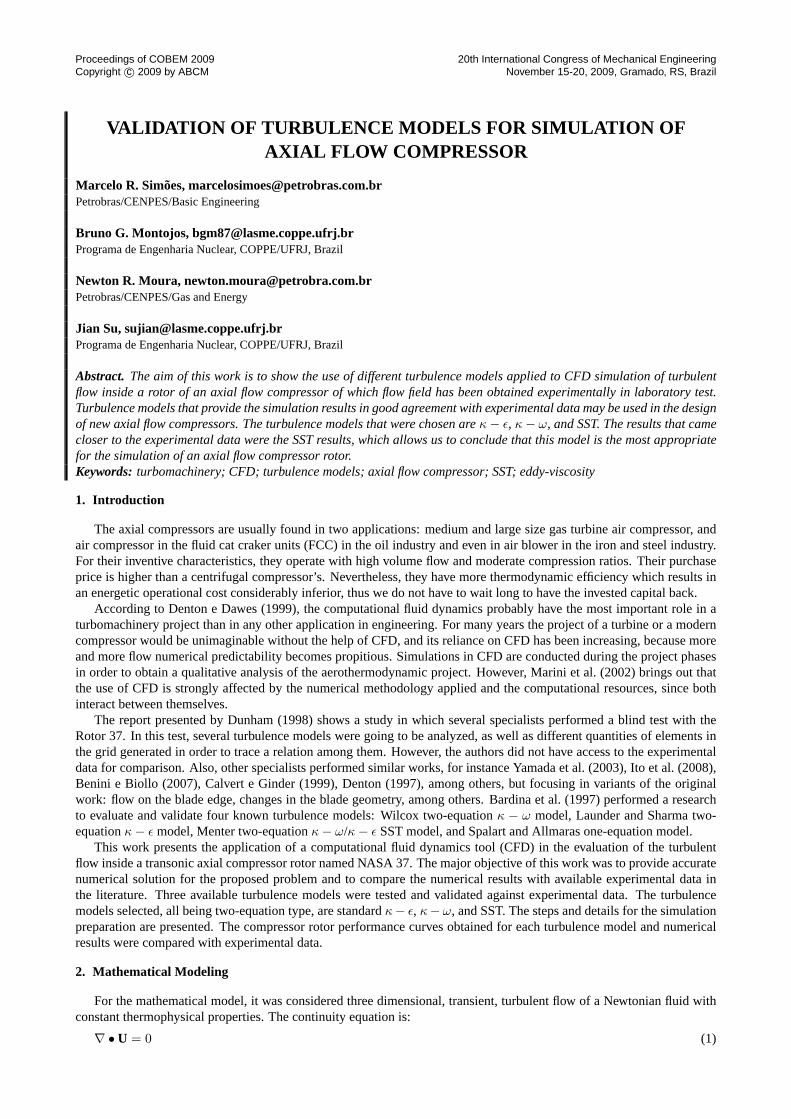
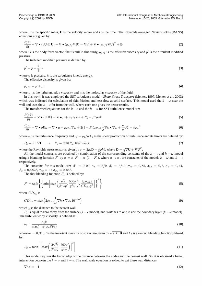
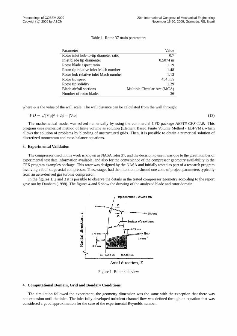
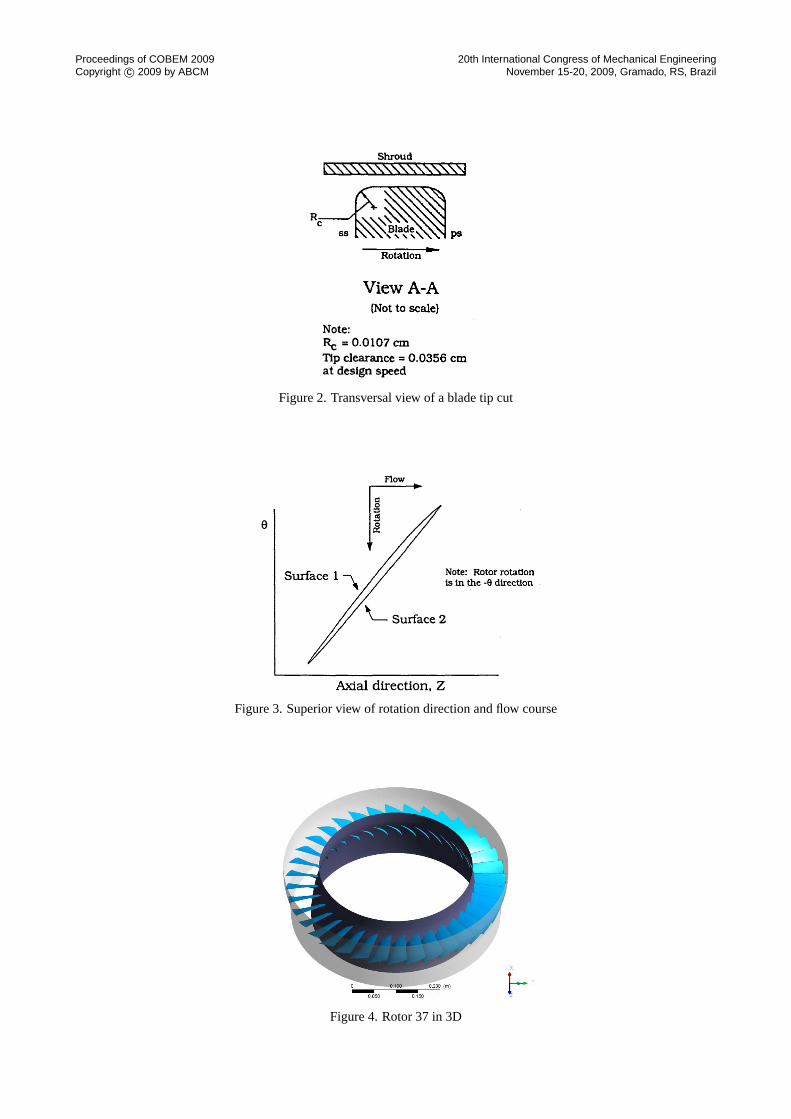
In the figures 1, 2 and 3 it is possible to observe the details in the tested compressor geometry according to the reportgave out by Dunham (1998). The figures 4 and 5 show the drawing of the analyzed blade and rotor domain.

Figure 1. Rotor side view

4. Computational Domain, Grid and Bondary Conditions

The simulation followed the experiment, the geometry dimension was the same with the exception that there wasnot extension until the inlet. The inlet fully developed turbulent channel flow was defined through an equation that wasconsidered a good approximation for the case of the experimental Reynolds number.



Figure 2. Transversal view of a blade tip cut

Figure 3. Superior view of rotation direction and flow course

Figure 4. Rotor 37 in 3D



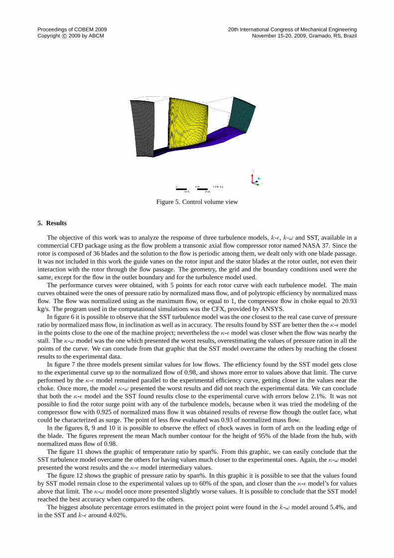
Figure 5. Control volume view

5. Results

The objective of this work was to analyze the response of three turbulence models,k-ε, k-ω and SST, available in acommercial CFD package using as the flow problem a transonic axial flow compressor rotor named NASA 37. Since therotor is composed of 36 blades and the solution to the flow is periodic among them, we dealt only with one blade passage.It was not included in this work the guide vanes on the rotor input and the stator blades at the rotor outlet, not even theirinteraction with the rotor through the flow passage. The geometry, the grid and the boundary conditions used were thesame, except for the flow in the outlet boundary and for the turbulence model used.

The performance curves were obtained, with 5 points for each rotor curve with each turbulence model. The maincurves obtained were the ones of pressure ratio by normalized mass flow, and of polytropic efficiency by normalized massflow. The flow was normalized using as the maximum flow, or equal to 1, the compressor flow in choke equal to 20.93kg/s. The program used in the computational simulations was the CFX, provided by ANSYS.

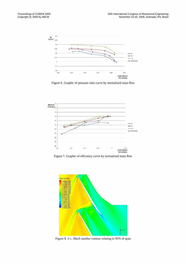
In figure 6 it is possible to observe that the SST turbulence model was the one closest to the real case curve of pressureratio by normalized mass flow, in inclination as well as in accuracy. The results found by SST are better then theκ-ε modelin the points close to the one of the machine project; nevertheless theκ-ε model was closer when the flow was nearby thestall. Theκ-ω model was the one which presented the worst results, overestimating the values of pressure ration in all thepoints of the curve. We can conclude from that graphic that the SST model overcame the others by reaching the closestresults to the experimental data.

In figure 7 the three models present similar values for low flows. The efficiency found by the SST model gets closeto the experimental curve up to the normalized flow of 0.98, and shows more error to values above that limit. The curveperformed by theκ-ε model remained parallel to the experimental efficiency curve, getting closer in the values near thechoke. Once more, the modelκ-ω presented the worst results and did not reach the experimental data. We can concludethat both theκ-ε model and the SST found results close to the experimental curve with errors below 2.1%. It was notpossible to find the rotor surge point with any of the turbulence models, because when it was tried the modeling of thecompressor flow with 0.925 of normalized mass flow it was obtained results of reverse flow though the outlet face, whatcould be characterized as surge. The point of less flow evaluated was 0.93 of normalized mass flow.

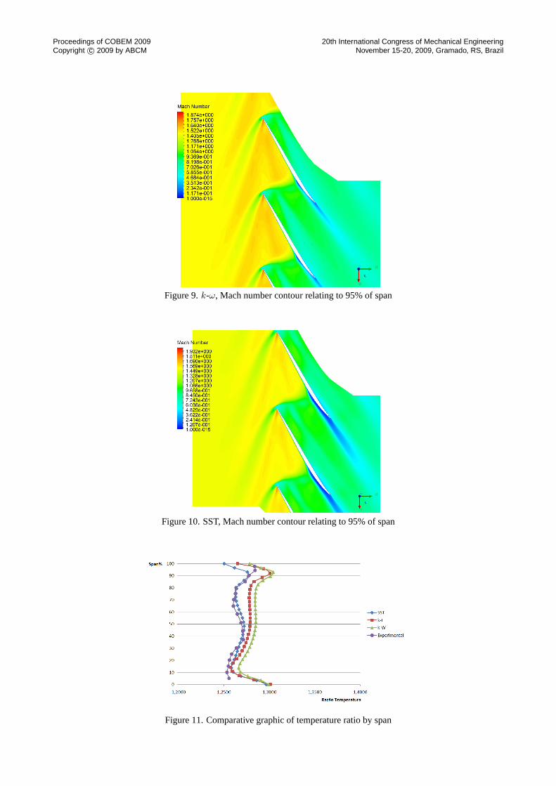
In the figures 8, 9 and 10 it is possible to observe the effect of chock waves in form of arch on the leading edge ofthe blade. The figures represent the mean Mach number contour for the height of 95% of the blade from the hub, withnormalized mass flow of 0.98.

The figure 11 shows the graphic of temperature ratio by span%. From this graphic, we can easily conclude that theSST turbulence model overcame the others for having values much closer to the experimental ones. Again, theκ-ω modelpresented the worst results and theκ-ε model intermediary values.

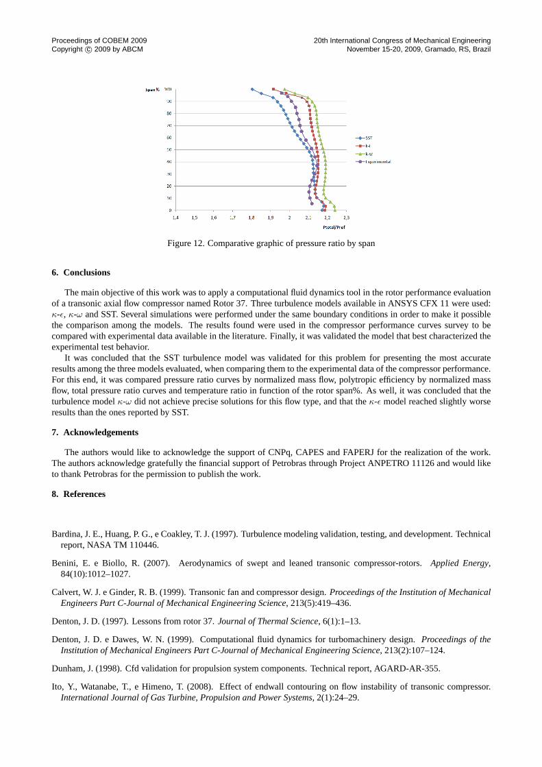
The figure 12 shows the graphic of pressure ratio by span%. In this graphic it is possible to see that the values foundby SST model remain close to the experimental values up to 60% of the span, and closer than theκ-ε model’s for valuesabove that limit. Theκ-ω model once more presented slightly worse values. It is possible to conclude that the SST modelreached the best accuracy when compared to the others.

The biggest absolute percentage errors estimated in the project point were found in thek-ω model around 5.4%, andin the SST andk-ε around 4.02%.



Figure 6. Graphic of pressure ratio curve by normalized mass flow

Figure 7. Graphic of efficiency curve by normalized mass flow

Figure 8.k-ε, Mach number contour relating to 95% of span



Figure 9.k-ω, Mach number contour relating to 95% of span

Figure 10. SST, Mach number contour relating to 95% of span

Figure 11. Comparative graphic of temperature ratio by span



Figure 12. Comparative graphic of pressure ratio by span

6. Conclusions

The main objective of this work was to apply a computational fluid dynamics tool in the rotor performance evaluationof a transonic axial flow compressor named Rotor 37. Three turbulence models available in ANSYS CFX 11 were used:κ-ε, κ-ω and SST. Several simulations were performed under the same boundary conditions in order to make it possiblethe comparison among the models. The results found were used in the compressor performance curves survey to becompared with experimental data available in the literature. Finally, it was validated the model that best characterized theexperimental test behavior.

It was concluded that the SST turbulence model was validated for this problem for presenting the most accurateresults among the three models evaluated, when comparing them to the experimental data of the compressor performance.For this end, it was compared pressure ratio curves by normalized mass flow, polytropic efficiency by normalized massflow, total pressure ratio curves and temperature ratio in function of the rotor span%. As well, it was concluded that theturbulence modelκ-ω did not achieve precise solutions for this flow type, and that theκ-ε model reached slightly worseresults than the ones reported by SST.

7. Acknowledgements

The authors would like to acknowledge the support of CNPq, CAPES and FAPERJ for the realization of the work.The authors acknowledge gratefully the financial support of Petrobras through Project ANPETRO 11126 and would liketo thank Petrobras for the permission to publish the work.

8. References

Bardina, J. E., Huang, P. G., e Coakley, T. J. (1997). Turbulence modeling validation, testing, and development. Technicalreport, NASA TM 110446.

Benini, E. e Biollo, R. (2007). Aerodynamics of swept and leaned transonic compressor-rotors.Applied Energy,84(10):1012–1027.

Calvert, W. J. e Ginder, R. B. (1999). Transonic fan and compressor design.Proceedings of the Institution of MechanicalEngineers Part C-Journal of Mechanical Engineering Science, 213(5):419–436.

Denton, J. D. (1997). Lessons from rotor 37.Journal of Thermal Science, 6(1):1–13.

Denton, J. D. e Dawes, W. N. (1999). Computational fluid dynamics for turbomachinery design.Proceedings of theInstitution of Mechanical Engineers Part C-Journal of Mechanical Engineering Science, 213(2):107–124.

Dunham, J. (1998). Cfd validation for propulsion system components. Technical report, AGARD-AR-355.

Ito, Y., Watanabe, T., e Himeno, T. (2008). Effect of endwall contouring on flow instability of transonic compressor.International Journal of Gas Turbine, Propulsion and Power Systems, 2(1):24–29.



Marini, M., Paoli, R., Grasso, F., Periaux, J., e Desideri, J. A. (2002). Verification and validation in computational fluiddynamics: the flownet database experience.Jsme International Journal Series B-Fluids and Thermal Engineering,45(1):15–22.

Menter, F. R. (1997). Eddy viscosity transport equations and their relation to thek-ε model.Journal of Fluid Engineering,119(3):876–884.

Menter, F. R., Kuntz, M., e Langtry, R. (2003). Ten years of industrial experience with the sst turbulence model. in K.Hanjalic, Y. Nagano e M. Tummers (eds.),Turbulence, Heat and Mass Transfer 4, Begell House, Inc.

Yamada, K., Furukawa, M., Inoue, M., e Funazaki, K.-I. (2003). Numerical analysis of tip leakage flow field ina atransonic axial compressor rotor. InProceedings of the International Gas Turbine Congress, Tokyo.

9. Responsibility notice

The authors are the only responsible for the printed material included in this paper

validation of turbulence models for simulation of axial flow …phoenics/em974/projetos/temas... ·...

Documents