v784 ophiuchi: an rr lyrae star with multiple blazhko ... · 214 de ponthiere et al., jaavso volume...

de Ponthiere et al., JAAVSO Volume 41, 2013214

V784 Ophiuchi: an RR Lyrae Star With Multiple Blazhko Modulations

Pierre de Ponthière15 Rue Pré Mathy, Lesve, Profondeville 5170, Belgium; address email correspondence to [email protected]

Franz-Josef Hambsch12 Oude Bleken, Mol, 2400, Belgium

Tom KrajciP.O. Box 1351, Cloudcroft, NM 88317

Kenneth Menzies318A Potter Road, Framingham, MA 01701

Received May 15, 2013; revised June 14, 2013; accepted June 24, 2013

Abstract The results of an observation campaign of V784 Ophiuchi over a time span of two years have revealed a multi-periodic Blazhko effect. A Blazhko effect for V784 Oph has not been reported previously. From the observed light curves, 60 pulsation maxima have been measured. The Fourier analyses of the (O–C) values and of magnitudes at maximum light (Mmax) have revealed a main Blazhko period of 24.51 days but also two other secondary Blazhko modulations with periods of 34.29 and 31.07 days. A complete light curve Fourier analysis with period04 has shown triplet structures based on main and secondary Blazhko frequencies close to the reciprocal of Blazhko periods measured from the 60 pulsation maxima.

1. Introduction

In the General Catalogue of Variable Stars (GCVS; Samus et al. 2011) V784 Ophiuchi is correctly classified as an RR Lyr (RRab) variable star but with an incorrect period of 0.3762746 day as pointed out by Wils et al. (2006). They corrected the period to 0.60336 day but did not detect a Blazhko effect from the Northern Sky Variability Survey data (Wozniak et al. 2004) due to the paucity of available datasets. The current data were gathered during 238 nights between June 2011 and October 2012. During this period of 488 days, a total of 15,223 magnitude measurements covering 18 Blazhko cycles were collected. The observations were made by Krajci and Hambsch using 30- and 40-cm telescopes located in Cloudcroft (New Mexico), Mol (Belgium), and mainly in San Pedro de Atacama (Chile). The numbers of observations for the different locations are 1,986 for Cloudcroft, 470 for Mol, and 12,767 for San Pedro de Atacama.

de Ponthiere et al., JAAVSO Volume 41, 2013 215

The comparison stars are given in Table 1. The star coordinates and magnitudes in B and V bands were obtained from the NOMAD catalogue (Zacharias et al. 2011). C1 was used as a magnitude reference and C2 as a check star. The Johnson V magnitudes from different instruments have not been transformed to the standard system since measurements were performed with a V filter only. However, two simultaneous maximum measurements from the instruments in Cloudcroft and San Pedro de Atacama were observed to differ by only 0.034 and 0.042 mag. Dark and flat field corrections were performed with maximdl software (Diffraction Limited 2004), and aperture photometry was performed using lesvephotometry (de Ponthière 2010), a custom software which also evaluates the SNR and estimates magnitude errors.

2. Light curve maxima analysis

The times of maxima of the light curves have been evaluated with custom software (de Ponthiere 2010) fitting the light curve with a smoothing spline function (Reinsch 1967). Table 2 provides the list of 60 observed maxima and Figures 1a and 1b show the (O–C) and Mmax (Magnitude at Maximum) values. For clarity only the most intensive part of the observation campaign is included in Figures 1a and 1b. From a simple inspection of the Mmax graph the Blazhko effect is obvious as well as the presence of a second modulation frequency. The Blazhko effect is itself apparently modulated by a lower frequency component. A linear regression of all available (O–C) values has provided a pulsation period of 0.6033557 d (1.657397 d–1). The (O–C) values have been re-evaluated with this new pulsation period and the pulsation ephemeris origin has been set to the highest recorded maximum: HJD 2456047.7942. The new derived pulsation elements are:

HJDPulsation = (2456047.7942 ± 0.0015) + (0.6033557 ± 0.0000078) EPulsation (1)

The derived pulsation period is in good agreement with the value of 0.60336 d published by Wils et al. (2006). The folded light curve on this pulsation period is shown in Figure 2. To determine the Blazhko effect, Fourier analyses and sine-wave fittings of the (O–C) values and Mmax (Magnitude at Maximum) values were performed with period04 (Lenz and Breger 2005). These analyses were limited to the first two frequency components and are tabulated in Table 3. The frequency uncertainties have been evaluated from the Least-Square fittings. The obtained periods (24.56 and 24.51 days) for the first Blazhko effect agree within the errors. However, the periods (34.29 and 31.07 days) of the second Blazhko modulation are statistically different and in the next section it will be shown that they are also found in the complete light curve Fourier analysis. To dismiss the possible effect of minor amplitude differences between


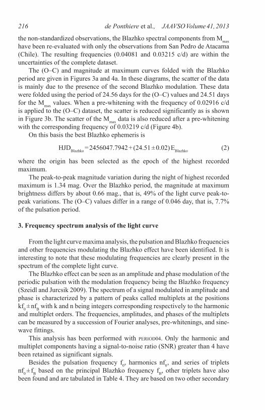
the non-standardized observations, the Blazhko spectral components from Mmax have been re-evaluated with only the observations from San Pedro de Atacama (Chile). The resulting frequencies (0.04081 and 0.03215 c/d) are within the uncertainties of the complete dataset. The (O–C) and magnitude at maximum curves folded with the Blazhko period are given in Figures 3a and 4a. In these diagrams, the scatter of the data is mainly due to the presence of the second Blazhko modulation. These data were folded using the period of 24.56 days for the (O–C) values and 24.51 days for the Mmax values. When a pre-whitening with the frequency of 0.02916 c/d is applied to the (O–C) dataset, the scatter is reduced significantly as is shown in Figure 3b. The scatter of the Mmax data is also reduced after a pre-whitening with the corresponding frequency of 0.03219 c/d (Figure 4b). On this basis the best Blazhko ephemeris is

HJDBlazhko = 2456047.7942 + (24.51 ± 0.02) EBlazhko (2)

where the origin has been selected as the epoch of the highest recorded maximum. The peak-to-peak magnitude variation during the night of highest recorded maximum is 1.34 mag. Over the Blazhko period, the magnitude at maximum brightness differs by about 0.66 mag., that is, 49% of the light curve peak-to-peak variations. The (O–C) values differ in a range of 0.046 day, that is, 7.7% of the pulsation period.

3. Frequency spectrum analysis of the light curve

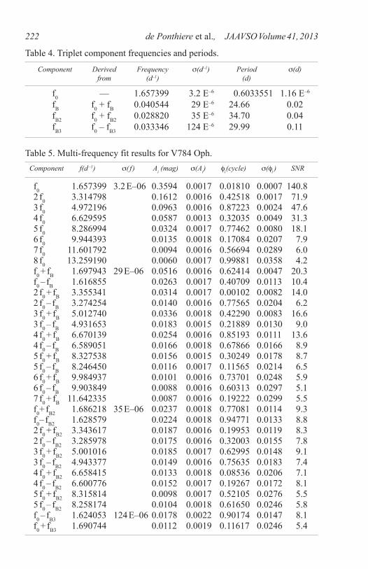
From the light curve maxima analysis, the pulsation and Blazhko frequencies and other frequencies modulating the Blazhko effect have been identified. It is interesting to note that these modulating frequencies are clearly present in the spectrum of the complete light curve. The Blazhko effect can be seen as an amplitude and phase modulation of the periodic pulsation with the modulation frequency being the Blazhko frequency (Szeidl and Jurcsik 2009). The spectrum of a signal modulated in amplitude and phase is characterized by a pattern of peaks called multiplets at the positions kf0 ± nfB with k and n being integers corresponding respectively to the harmonic and multiplet orders. The frequencies, amplitudes, and phases of the multiplets can be measured by a succession of Fourier analyses, pre-whitenings, and sine-wave fittings. This analysis has been performed with period04. Only the harmonic and multiplet components having a signal-to-noise ratio (SNR) greater than 4 have been retained as significant signals. Besides the pulsation frequency f0, harmonics nf0, and series of triplets nf0 ± fB based on the principal Blazhko frequency fB, other triplets have also been found and are tabulated in Table 4. They are based on two other secondary


modulation frequencies, fB2 and fB3, which are close to the secondary modulation components identified in the (O–C) and Mmax analyses. It is interesting to note that the period (1/fB2) of 34.70 days is close to the second period 34.29 days found in the (O–C) analysis. The period (1/fB3) of 29.99 days can be compared to the second period 31.07 days found in the magnitude at maximum (Mmax) analysis. Table 5 provides the complete list of Fourier components with their amplitudes, phases, and uncertainties. During the sine-wave fitting, the fundamental frequency f0 and largest triplets f0 + fB, f0 + fB2, and f0 – fB3 have been left unconstrained and the other frequencies have been entered as combinations of these four frequencies. The uncertainties of frequencies, amplitudes, and phases have been estimated by Monte Carlo simulations. The amplitude and phase uncertainties have been multiplied by a factor of two as it is known that the Monte Carlo simulations underestimate these uncertainties (Kolenberg et al. 2009). The two Blazhko modulation frequencies, fB (0.040544) and fB2 (0.028820), are close to a 7:5 resonance ratio and the corresponding beat period is around 173 days. Calculations based on Blazhko periods (24.56 and 34.29 days) obtained with the (O–C) analysis provide the same resonance ratio. The other pair of frequencies, fB (0.040544) and fB3 (0.033346), is close to a 5:6 resonance ratio with a beat period around 149 days, but a different resonance ratio of 5:4 with a beat period of 123 days is obtained from the periods (24.51 and 31.07 days) found in the Mmax analysis. This discrepancy is probably due to the greater uncertainty (124 E–6) of the fB3 side lobes. In CZ Lacertae, Sódor et al. (2011) have also detected two modulation components with a resonance ratio of 5:4 during a first observing season but a different resonance ratio of 4:3 during the next season. Table 6 lists for each harmonic the amplitude ratios Ai/A1 and the ratios usually used to characterize the Blazhko effect, that is, Ai

+/A1 ; Ai–/A1 ; Ri = A+

i1 / A–

i1; and asymmetries Qi = (A+i1 – A–

i1) / (A+i1 + A–

i1). Szeidl and Jurcsik (2009) have shown that the asymmetry of the side lobe amplitudes depends on the phase difference between the amplitude and the phase modulation. If the Blazhko effect is limited to amplitude or phase modulation the asymmetry vanishes. In the present case the side lobe A+

i1 is the strongest one, which is generally the case for stars showing a Blazhko effect. The asymmetry ratios Qi around 0.32 are a sign of both strong amplitude and phase modulations. The Ri and Qi ratios for triplets around the secondary Blazhko frequency fB2 are also given in Table 6. The fB2 frequency is close to the secondary frequency detected in the (O–C) analysis and thus likely related to a phase modulation effect. The fB2 frequency seems to act only on phase modulation, and this could explain the low asymmetry values (0.03) of the fB2 side lobes.

4. Light curve variations over Blazhko cycle

Subdividing the data set into temporal subsets is a classical method to


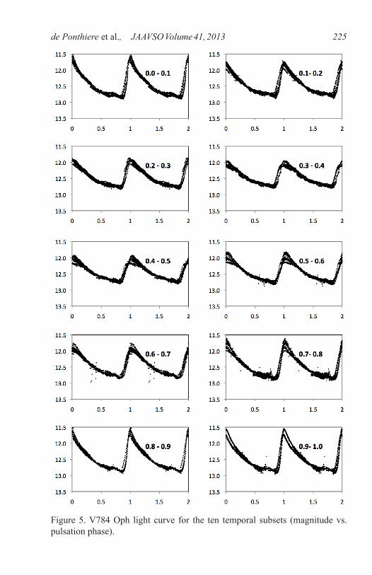
analyze the light curve variations over the Blazhko cycle. Ten temporal subsets corresponding to the different Blazhko phase intervals Yi (i = 0 , 9) have been created using the epoch of the highest recorded maximum (2456047.7942) as the origin of the first subset. Fortunately, the data points are relatively well distributed over the subsets with the number of data points varying between 1,126 and 1,715. Figure 5 presents the folded light curve for the ten subsets. Despite the subdivision over the Blazhko cycle, a scatter still remains in the light curves. The light curves are folded with the primary Blazhko frequency, and the secondary Blazhko frequencies are creating the observed scatter. Fourier analyses and Least-Square fittings have been performed on the different temporal subsets. For the fundamental and the first four harmonics the amplitude Ai and the epoch-independent phase differences (Fk1 = Fk – kF1) are given in Table 7 and plotted in Figure 6. The number of data points belonging to each subset is also given in this table. The amplitudes of the fundamental and harmonics show smooth sinusoidal variations with the minima occurring around Blazhko phase 0.5, that is, when the light curve amplitude variation on the pulsation is weaker. The ratio of harmonic A4 to fundamental A1 is at maximum at Blazhko phase 1.0, when the ascending branch of the light curve is steeper. The difference between maximum and minimum F1 phases is a measure of the phase modulation strength and is equal to 0.453 radian, or 0.072 cycle, which corresponds roughly to the value of 7.7% noted for the peak-to-peak deviation of (O–C). The epoch-independent phase differences F

31 and F

41 vary as smooth sinusoids, with the maximum phase differences occurring at Blazhko phase 0.5. However, F

21 variations, if any, are small. This weak F21

variation has been also noted for MW Lyr (Jurcsik et al. 2008) and V1820 Ori (de Ponthiere et al. 2013).

5. Conclusions

The effects of three Blazhko modulations have been detected by measurements of (O–C) values and amplitude of light curve maxima and confirmed by complete light curve Fourier analysis. The main Blazhko period (1 / fB) is 24.51 days. The secondary Blazhko period (1 / fB2) of 34.70 days is apparently related to phase modulation, as it is detected in the (O–C) analysis, and fB and fB2 are close to a 7:5 resonance ratio. The tertiary modulation (1 / fB3) is weaker in the Fourier analysis and the period values are slightly different from magnitude at maximum and light curve Fourier analysis (31.07 and 29.99 days, respectively). The resonance ratios of fB and fB3 are approximately 5:4 or 5:6 in function of the analysis method. This discrepancy is probably due to the weakness of the corresponding Fourier multiplet values and their larger uncertainties.


6. Acknowledgements

AAVSO Director Dr. Arne A. Henden and the AAVSO are acknowledged for the use of AAVSOnet telescopes at Cloudcroft (New Mexico). The authors thank the referee for constructive comments which have helped to clarify and improve the paper. This work has made use of The International Variable Star Index (VSX) maintained by the AAVSO and of the SIMBAD astronomical database (http://simbad.u-strasbg.fr)

References

de Ponthière, P. 2010, lesvephotometry, automatic photometry software (http://www.dppobservatory.net).

de Ponthière, P. , Hambsch, F.-J., Krajci, T., Menzies, K., and Wils, P. 2013, J. Amer. Assoc. Var. Star Obs., 41, 58.

Diffraction Limited. 2004, maximdl image processing software (http://www.cyanogen.com).

Jurcsik, J., et al. 2008, Mon. Not. Roy. Astron. Soc., 391, 164.Kolenberg, K., et al. 2009, Mon. Not. Roy. Astron. Soc., 396, 263.Lenz, P., and Breger, M. 2005, Commun. Asteroseismology, 146, 53.Reinsch, C. H. 1967, Numer. Math., 10, 177.Samus, N. N., et al. 2011, General Catalogue of Variable Stars (GCVS database,

Version 2011 January, http://www.sai.msu.su/gcvs/gcvs/index.htm).Sódor, Á., et al. 2011, Mon. Not. Roy. Astron. Soc., 411, 1585.Szeidl, B., and Jurcsik, J. 2009, Commun. Asteroseismology, 160, 17.Wils, P., Lloyd, C., and Bernhard, K. 2006, Mon. Not. Roy. Astron. Soc., 368, 1757.Wozniak, P., et al. 2004, Astron. J., 127, 2436.Zacharias, N., Monet, D., Levine, S., Urban, S., Gaume, R., and Wycoff, G.

2011, The Naval Observatory Merged Astrometric Dataset (NOMAD, http://www.usno.navy.mil/USNO/astrometry/optical-IR-prod/nomad/the-nomad1-catalogue).

Table 1. Comparison stars for V784 Oph. Identification R. A. (2000) Dec. (2000) B V B–V h m s ° ' "

GSC 992-1617 17 35 18.037 +07 40 58.97 13.24 12.32 0.92 C1 TYC 992-1203 17 35 35.883 +07 41 29.21 11.491 10.442 1.049 C2


Table 2. List of measured maxima of V784 Oph.

Maximum HJD Error O–C (day) E Magnitude Error Location*

2455778.6910 0.0014 –0.0066 –446 11.692 0.004 1 2455780.5024 0.0021 –0.0052 –443 11.841 0.004 1 2455783.5146 0.0035 –0.0098 –438 12.043 0.005 1 2455792.5913 0.0055 0.0166 –423 11.952 0.022 1 2455795.6064 0.0023 0.0149 –418 11.757 0.005 1 2455798.6121 0.0022 0.0038 –413 11.581 0.004 1 2455801.6283 0.0012 0.0032 –408 11.580 0.004 1 2455804.6413 0.0018 –0.0006 –403 11.747 0.004 1 2455815.5203 0.0062 0.0180 –385 12.139 0.005 1 2455818.5302 0.0040 0.0112 –380 11.998 0.005 1 2455989.8824 0.0030 0.0103 –96 11.897 0.006 1 2455992.8923 0.0021 0.0035 –91 11.762 0.007 1 2456009.8043 0.0036 0.0215 –63 11.971 0.008 1 2456012.8109 0.0027 0.01133 –58 11.830 0.007 1 2456015.8195 0.0018 0.00315 –53 11.683 0.006 1 2456018.8292 0.0015 –0.00393 –48 11.569 0.006 1 2456024.8557 0.0014 –0.01098 –38 11.751 0.009 1 2456027.8774 0.0026 –0.00606 –33 11.965 0.009 1 2456035.7338 0.0025 0.00671 –20 12.028 0.007 1 2456038.7570 0.0033 0.01314 –15 11.898 0.007 1 2456038.7570 0.0033 0.01314 –15 11.898 0.007 1 2456047.7942 0.0019 0.00000 0 11.512 0.006 1 2456050.8100 0.0019 –0.00098 5 11.753 0.007 1 2456053.8208 0.0025 –0.00696 10 11.931 0.010 1 2456056.8352 0.0041 –0.00934 15 12.120 0.008 1 2456059.8458 0.0071 –0.01551 20 12.172 0.011 1 2456062.8785 0.0082 0.00041 25 12.091 0.007 1 2456064.6946 0.0034 0.00644 28 11.939 0.007 1 2456065.8972 0.0029 0.00233 30 11.856 0.008 1 2456067.7028 0.0019 –0.00214 33 11.709 0.007 1 2456068.9082 0.0009 –0.00345 35 11.624 0.008 1 2456070.7195 0.0016 –0.00222 38 11.555 0.006 1 2456073.7360 0.0014 –0.00249 43 11.563 0.007 1 2456076.7611 0.0021 0.00583 48 11.764 0.007 1 2456076.7625 0.0032 0.00723 48 11.806 0.015 2 2456079.7870 0.0026 0.01495 53 11.922 0.008 1 2456081.6018 0.0037 0.01968 56 11.980 0.010 1 2456082.8111 0.0090 0.02227 58 12.060 0.013 1 2456084.6218 0.0046 0.02290 61 12.036 0.010 1

Table continued on next page


Table 2. List of measured maxima of V784 Oph, cont.

Maximum HJD Error O–C (day) E Magnitude Error Location*

2456085.8238 0.0052 0.01819 63 12.044 0.009 1 2456087.6345 0.0045 0.01882 66 11.997 0.008 1 2456088.8314 0.0043 0.00901 68 11.966 0.008 1 2456088.8321 0.0045 0.00971 68 12.000 0.012 2 2456091.8378 0.0024 –0.00137 73 11.906 0.013 2 2456093.6474 0.0026 –0.00183 76 11.771 0.007 1 2456096.6554 0.0015 –0.01061 81 11.712 0.007 1 2456102.6891 0.0051 –0.01047 91 11.870 0.012 2 2456105.7166 0.0036 0.00025 96 11.961 0.010 2 2456108.7536 0.0033 0.02048 101 11.932 0.009 1 2456110.5743 0.0040 0.03111 104 11.895 0.010 1 2456111.7694 0.0030 0.01950 106 11.824 0.012 1 2456113.5785 0.0027 0.01853 109 11.783 0.010 1 2456114.7832 0.0024 0.01652 111 11.727 0.009 1 2456116.5854 0.0012 0.00865 114 11.631 0.007 1 2456122.6012 0.0018 –0.00911 124 11.673 0.006 1 2456125.6160 0.0028 –0.01108 129 11.821 0.007 1 2456131.6492 0.0068 –0.01144 139 12.059 0.008 1 2456134.6806 0.0037 0.00318 144 11.988 0.008 1 2456145.5391 0.0008 0.00128 162 11.572 0.007 1 2456227.5864 0.0027 –0.00780 298 11.955 0.006 2* Locations : 1—San Pedro de Atacama (Chile); 2—Cloudcroft (New Mexico).

Table 3. Blazhko spectral components.

From (O–C) values

Frequency s(d–1) Period s(d) Amplitude f (cycle/days) (days) (days) (cycle)

0.04071 13 E–5 24.56 0.08 0.0098 0.502 0.02916 14 E–5 34.29 0.17 0.0091 0.195

From Mmax

Frequency s(d–1) Period s(d) Amplitude f (cycle/days) (days) (mag.) (cycle)

0.04080 4 E–5 24.51 0.02 0.229 0.622 0.03219 8 E–5 31.07 0.08 0.112 0.620


Table 4. Triplet component frequencies and periods.

Component Derived Frequency s(d–1) Period s(d) from (d–1) (d)

f0 — 1.657399 3.2 E–6 0.6033551 1.16 E–6

fB f0 + fB 0.040544 29 E–6 24.66 0.02 fB2 f0 + fB2 0.028820 35 E–6 34.70 0.04 fB3 f0 – fB3 0.033346 124 E–6 29.99 0.11

f0 1.657399 3.2 E–06 0.3594 0.0017 0.01810 0.0007 140.8 2 f0 3.314798 0.1612 0.0016 0.42518 0.0017 71.9 3 f0 4.972196 0.0963 0.0016 0.87223 0.0024 47.6 4 f0 6.629595 0.0587 0.0013 0.32035 0.0049 31.3 5 f0 8.286994 0.0324 0.0017 0.77462 0.0080 18.1 6 f0 9.944393 0.0135 0.0018 0.17084 0.0207 7.9 7 f0 11.601792 0.0094 0.0016 0.56694 0.0289 6.0 8 f0 13.259190 0.0060 0.0017 0.99881 0.0358 4.2 f0 + fB 1.697943 29 E–06 0.0516 0.0016 0.62414 0.0047 20.3 f0 – fB 1.616855 0.0263 0.0017 0.40709 0.0113 10.4 2 f0 + fB 3.355341 0.0314 0.0017 0.00102 0.0082 14.0 2 f0 – fB 3.274254 0.0140 0.0016 0.77565 0.0204 6.2 3 f0 + fB 5.012740 0.0336 0.0018 0.42290 0.0083 16.6 3 f0 – fB 4.931653 0.0183 0.0015 0.21889 0.0130 9.0 4 f0 + fB 6.670139 0.0254 0.0016 0.85193 0.0111 13.6 4 f0 – fB 6.589051 0.0166 0.0018 0.67866 0.0166 8.9 5 f0 + fB 8.327538 0.0156 0.0015 0.30249 0.0178 8.7 5 f0 – fB 8.246450 0.0116 0.0017 0.11565 0.0214 6.5 6 f0 + fB 9.984937 0.0101 0.0016 0.73701 0.0248 5.9 6 f0 – fB 9.903849 0.0088 0.0016 0.60313 0.0297 5.1 7 f0 + fB 11.642335 0.0087 0.0016 0.19222 0.0299 5.5 f0+ fB2 1.686218 35 E–06 0.0237 0.0018 0.77081 0.0114 9.3 f0– fB2 1.628579 0.0224 0.0018 0.94771 0.0133 8.8 2 f0 + fB2 3.343617 0.0187 0.0016 0.19953 0.0119 8.3 2 f0 – fB2 3.285978 0.0175 0.0016 0.32003 0.0155 7.8 3 f0 + fB2 5.001016 0.0185 0.0017 0.62995 0.0148 9.1 3 f0 – fB2 4.943377 0.0149 0.0016 0.75635 0.0183 7.4 4 f0 + fB2 6.658415 0.0133 0.0018 0.08536 0.0206 7.1 4 f0 – fB2 6.600776 0.0152 0.0017 0.19267 0.0172 8.1 5 f0 + fB2 8.315814 0.0098 0.0017 0.52105 0.0276 5.5 5 f0 – fB2 8.258174 0.0104 0.0018 0.61650 0.0246 5.8 f0 – fB3 1.624053 124 E–06 0.0178 0.0022 0.90174 0.0147 8.1 f0 + fB3 1.690744 0.0112 0.0019 0.11617 0.0246 5.4

Table 5. Multi-frequency fit results for V784 Oph. Component f(d –1) s( f ) Ai (mag) s(Ai) fi(cycle) s(fi ) SNR


1 1.00 0.14 0.07 1.96 0.32 1.06 0.03 2 0.45 0.09 0.04 2.24 0.38 1.07 0.03 3 0.27 0.09 0.05 1.84 0.30 1.24 0.11 4 0.16 0.07 0.05 1.53 0.21 0.88 –0.07 5 0.09 0.04 0.03 1.35 0.15 0.94 –0.03 6 0.04 0.03 0.02 1.15 0.07 — — 7 0.03 0.02 — — — — — 8 0.02 — — — — — —

Table 6. V784 Oph harmonic, triplet amplitudes, ratios, and asymmetry parameters. i Ai/A1 Ai

+/A1 Ai–/A1 Ri Qi Ri (fB2) Qi (fB2)

0.0–0.1 0.423 0.191 0.137 0.093 0.220 0.161 2.406 5.024 1.357 0.1–0.2 0.363 0.162 0.102 0.064 0.176 0.025 2.392 5.126 1.432 0.2–0.3 0.324 0.144 0.085 0.055 0.170 0.383 2.458 5.300 1.724 0.3–0.4 0.293 0.123 0.059 0.042 0.145 0.399 2.533 5.417 2.140 0.4–0.5 0.288 0.114 0.050 0.027 0.094 0.248 2.533 5.631 2.338 0.5–0.6 0.322 0.133 0.066 0.036 0.111 0.287 2.536 5.411 2.010 0.6–0.7 0.354 0.154 0.077 0.041 0.117 0.168 2.477 5.276 1.949 0.7–0.8 0.394 0.174 0.119 0.072 0.182 0.067 2.457 5.166 1.518 0.8–0.9 0.408 0.197 0.138 0.101 0.246 0.202 2.415 5.121 1.466 0.9–1.0 0.431 0.196 0.149 0.096 0.223 -0.054 2.234 4.797 1.127

Table 7. V784 Oph Fourier coefficients over Blazhko cycles. Y A1 A2 A3 A4 A4 / A1 F1 F21 F31 F41 (cycle) (mag) (mag) (mag) (mag) (rad) (rad) (rad) (rad)

Figure 1a, b. V784 Oph O–C (days) and magnitude at maximum.


Figure 2. V784 Oph light curve folded with pulsation period.

Figure 3a. O–C without pre-whitening.

Figure 3b. O–C after pre-whitening.

Figure 4a. Magnitude at maximum without pre-whitening.

Figure 4b. Magnitude at maximum after pre-whitening.


Figure 5. V784 Oph light curve for the ten temporal subsets (magnitude vs. pulsation phase).


Figure 6a. V784 Oph Fourier Ai amplitude (mag.) for the ten temporal subsets.

Figure 6b. V784 Oph Fourier Fi and Fki phase (rad.) for the ten temporal subsets.

v784 ophiuchi: an rr lyrae star with multiple blazhko ... · 214 de ponthiere et al., jaavso volume...

Documents