v. 10 - aquaveogmstutorials-10.0.aquaveo.com/seep2d-sheetpile.pdf · gms 10.0 tutorial seep2d –...
TRANSCRIPT

Page 1 of 13 © Aquaveo 2015
GMS 10.0 Tutorial
SEEP2D – Sheet Pile Use SEEP2D to create a flow net around a sheet pile
Objectives Learn how to set up and solve a seepage problem involving flow around a sheet pile using the SEEP2D
interface in GMS.
Prerequisite Tutorials Feature Objects
Required Components GIS
Map Module
Mesh Module
SEEP2D
Time 30–45 minutes
v. 10.0
Page 2 of 13 © Aquaveo 2015
1 Introduction ......................................................................................................................... 2 1.1 Outline .......................................................................................................................... 2
2 Description of Problem ....................................................................................................... 2 3 Program Mode..................................................................................................................... 3 4 Getting Started .................................................................................................................... 4 5 Setting the Units .................................................................................................................. 4 6 Saving the Project ............................................................................................................... 5 7 Creating the Conceptual Model Features ......................................................................... 5
7.1 Defining a Coordinate System ...................................................................................... 5 7.2 Creating the Corner Points ........................................................................................... 6 7.3 Creating the Arcs .......................................................................................................... 7 7.4 Creating the Polygons .................................................................................................. 9 7.5 Assigning the Material Properties and Zones ............................................................. 10
8 Assigning Boundary Conditions ...................................................................................... 11 8.1 Constant Head Boundaries ......................................................................................... 11 8.2 Building the Finite Element Mesh .............................................................................. 12
9 Running SEEP2D .............................................................................................................. 13 10 Conclusion.......................................................................................................................... 13
1 Introduction
SEEP2D is a 2D, finite-element, steady-state flow model. It is typically used for profile
models (i.e., cross-section models representing a vertical slice through a flow system that
is symmetric in the third dimension). Examples include earth dams, levees, sheet piles,
etc.
1.1 Outline
Follow these steps to complete this tutorial:
1. Create a SEEP2D conceptual model.
2. Map the model to a 2D mesh.
3. Run SEEP2D.
4. View the solution.
2 Description of Problem
The problem in this tutorial is shown in Figure 1

GMS Tutorials SEEP2D – Sheet Pile
Page 3 of 13 © Aquaveo 2015
Kx = Ky = 30 m/yr10 m
30 m 20 m
3 m10 m
3 m
Figure 1 Confined flow problem
The problem involves a partially penetrating sheet pile wall with an impervious clay
blanket on the upstream side. The sheet pile is driven into a silty sand deposit underlain
by bedrock at a depth of 10 m.
From a SEEP2D viewpoint, this problem is a “confined” problem. For SEEP2D, a
problem is confined if it is completely saturated. A problem is unconfined if it is partially
saturated.
3 Program Mode
The GMS interface can be modified by selecting a Program Mode. When the user first
installs and runs GMS, it is in the standard or “GMS” mode, which provides access to
the complete GMS interface, including all of the MODFLOW tools. The “GMS 2D”
mode provides a greatly simplified interface to the SEEP2D and UTEXAS codes. This
mode hides all of the tools and menu commands not related to SEEP2D and UTEXAS.
This tutorial assumes that the user is operating in the GMS 2D mode. Once the mode is
changed, the user can exit and restart GMS repeatedly and the interface stays in the same
mode until the user changes it back. Thus, the user only needs to change the mode once
if the user intends to repeatedly solve SEEP2D/UTEXAS problems. If the user is already
in GMS 2D mode, skip ahead to the next section. If the user is not already in GMS 2D
mode, do the following:
1. Launch GMS.
2. Select the Edit | Preferences command.
3. Select the Program Mode option on the left side of the dialog.
4. On the right side of the dialog, change the mode to “GMS 2D.”
5. Click on the OK button.

GMS Tutorials SEEP2D – Sheet Pile
Page 4 of 13 © Aquaveo 2015
6. Click Yes in response to the warning.
7. Click OK to get rid of the New Project dialog.
8. Then select the File | Exit command to exit GMS.
4 Getting Started
Do the following to get started:
1. If necessary, launch GMS.
2. If GMS is already running, select the File | New command to ensure that the
program settings are restored to their default state.
At this point, the user should see the New Project dialog. This dialog is used to set up a
GMS conceptual model. A conceptual model is a set of GIS features (points, lines, and
polygons) that are used to define the model input. The data in the conceptual model are
organized into a set of layers or groups called “coverages.” Each coverage is used to
define a portion of the input, and the properties that are assigned to the features in a
coverage are dependent on the coverage type. GMS 2D allows the user to quickly and
easily define all of the coverages needed for the conceptual model using the New Project
dialog. Most of the options the user sees in the window are related to UTEXAS. For
SEEP2D models, the only necessary coverage is the Profile lines coverage. This allows
the user to define the geometry of the mesh, the boundary conditions, and the material
zones.
3. Change the Conceptual model name to “Sheetpile Model.”
4. Turn off the UTEXAS option in the Numerical models section.
5. Make sure the Profile lines option is still selected.
6. Click OK.
The user should see a new conceptual model object appear in the Project Explorer.
5 Setting the Units
Before continuing, the user will establish the units to be used. GMS will display the
appropriate units label next to each of the input fields to remind the user to be sure to use
consistent units.
1. Select the Edit | Units command.
2. For the length select the “…” button.
3. Change the units for both horizontal and vertical to “meters.”

GMS Tutorials SEEP2D – Sheet Pile
Page 5 of 13 © Aquaveo 2015
4. Select “yr” for the Time units.
5. Select “kg” for the Mass units.
6. Select the OK button.
6 Saving the Project
Before continuing, save the project as a GMS project file.
1. Select the File | Save As command.
2. Navigate to the \Tutorials\SEEP2D directory.
3. Change the name of the project file to “s2con.”
4. Click on the Save button.
Click on the Save macro frequently to save all changes.
7 Creating the Conceptual Model Features
The first step in setting up the problem is to create the GIS features defining the problem
geometry. The user will begin by entering a set of points corresponding to the key
locations in the geometry. The user will then connect the points with lines called “arcs”
to define the outline of the problem. The user will next convert the arcs to a closed
polygon defining the problem domain. Once this is complete, the arcs and the polygon
will be used to build the finite element mesh and define the boundary conditions to the
problem.
7.1 Defining a Coordinate System
Before constructing the conceptual model features, the user must first establish a
coordinate system. The user will use a coordinate system with the origin 30 meters
upstream of the sheet pile at the top of the bedrock as shown in Figure 2.

GMS Tutorials SEEP2D – Sheet Pile
Page 6 of 13 © Aquaveo 2015
(0, 10)
(0, 0)
(20, 10)
(30, 10)
(30, 7)
(50, 10)
(50, 0)
Figure 2 Coordinate system
7.2 Creating the Corner Points
It is now possible to create some points at key corner locations. These points will then be
used to guide the construction of a set of arcs defining the model boundary.
1. Right-click on the “Profile lines” coverage in the Project Explorer.
2. Select the Attribute Table command to open the Attribute Table dialog.
3. Enter the following coordinates in the spreadsheet.
X Y
0 0
0 10
20 10
30 10
30 7
30.3 10
30.3 7
50 10
50 0
4. Click OK to exit the dialog.
5. Now select the Frame macro to center the view on the new points.
If the user needs to edit the node coordinates, this can be done by using the Select
Points/Nodes tool. When this tool is active, the user can select points and change the
coordinates using the edit fields at the top of the GMS window. The user can also select
points and delete them using the Delete key on the keyboard or the Delete command in
the Edit menu.
The user has entered points at 30, 10 and at 30.3, 10. The user has done this to model the
sheet pile which is about 0.3 m thick.
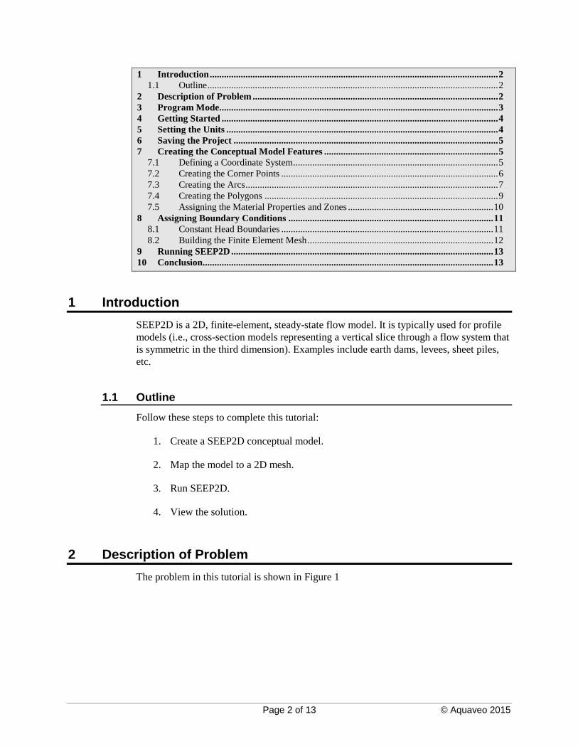
The nodes that were created should resemble the nodes shown in Figure 3.
GMS Tutorials SEEP2D – Sheet Pile
Page 7 of 13 © Aquaveo 2015
Figure 3. Points created in the profile lines coverage.
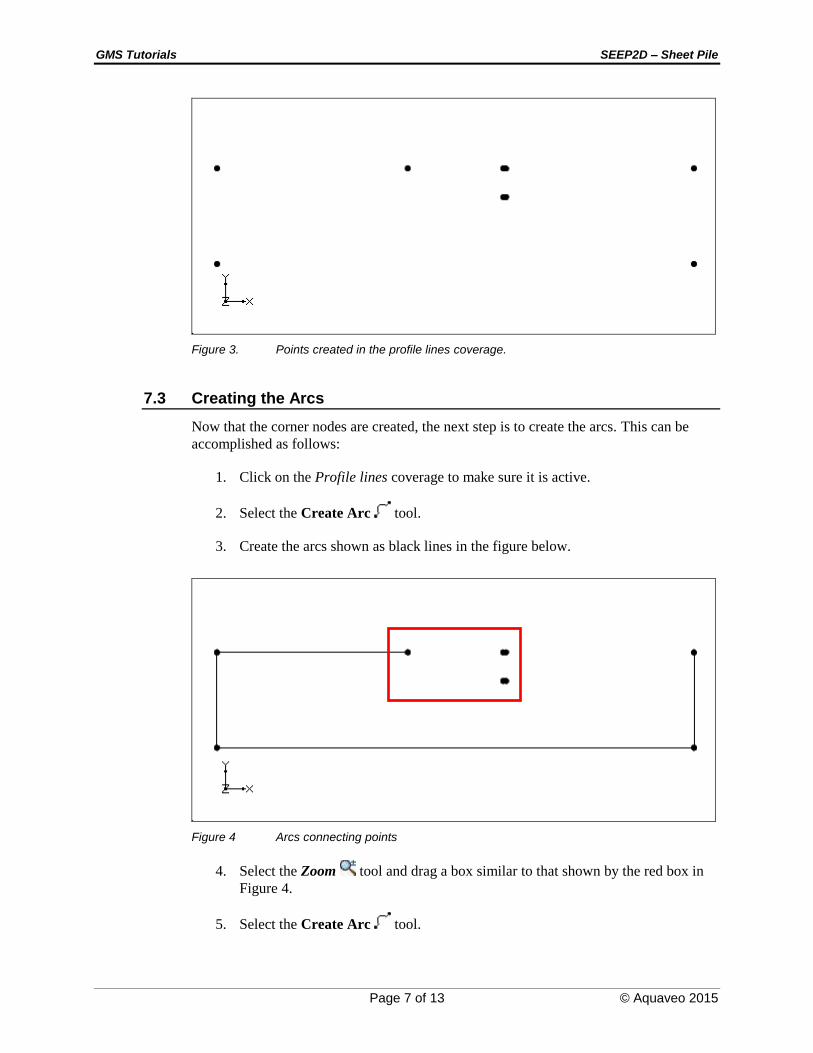
7.3 Creating the Arcs
Now that the corner nodes are created, the next step is to create the arcs. This can be
accomplished as follows:
1. Click on the Profile lines coverage to make sure it is active.
2. Select the Create Arc tool.
3. Create the arcs shown as black lines in the figure below.
Figure 4 Arcs connecting points
4. Select the Zoom tool and drag a box similar to that shown by the red box in
Figure 4.
5. Select the Create Arc tool.
GMS Tutorials SEEP2D – Sheet Pile
Page 8 of 13 © Aquaveo 2015
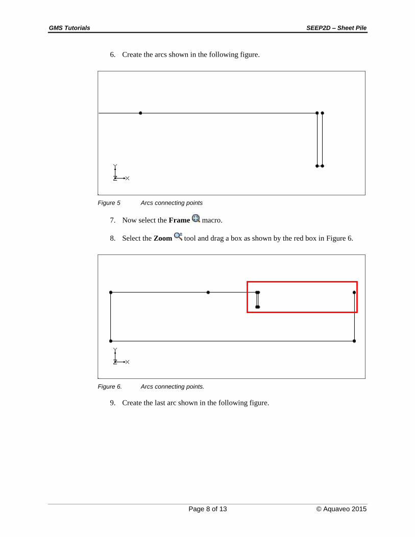
6. Create the arcs shown in the following figure.
Figure 5 Arcs connecting points
7. Now select the Frame macro.
8. Select the Zoom tool and drag a box as shown by the red box in Figure 6.
Figure 6. Arcs connecting points.
9. Create the last arc shown in the following figure.

GMS Tutorials SEEP2D – Sheet Pile
Page 9 of 13 © Aquaveo 2015
Figure 7 Arcs connecting points
10. Now select the Frame macro.
11. The model should now look like Figure 8.
Figure 8 Arcs connecting points
7.4 Creating the Polygons
Now that the arcs are created, the user can use the arcs to build a polygon representing
the region enclosed by the arcs. For problems with multiple materials, use the polygons
to assign the material zones. The user only has one material in this case, but it is still
necessary to create a polygon. To build the polygon, do the following:
1. Select the Feature Objects | Build Polygons command.
The user should see a polygon appear in the background.

GMS Tutorials SEEP2D – Sheet Pile
Page 10 of 13 © Aquaveo 2015
7.5 Assigning the Material Properties and Zones
Next, the user will assign the material properties and zones. To edit the material
properties, do the following:
1. Click on the Materials icon at the top of the GMS window.
2. Make sure the SEEP2D tab is selected.
At this point, the user would normally create a material for each of the zones in the
problem and give each material a unique name and color. But since the user has only one
material, the user can use the default name and color and simply edit the properties. The
material properties are k1, k2, and an angle. The values k1 and k2 represent the two
principal hydraulic conductivities and the angle is the angle from the x-axis to the
direction of the major principle hydraulic conductivity measured counter-clockwise as
shown in Figure 9.
y
x
a
k2
k1
Figure 9 Definition of hydraulic conductivity angle
With most natural soil deposits, the major principal hydraulic conductivity is in the x
direction, the minor principal hydraulic conductivity is in the y direction, and the angle is
zero. The units for hydraulic conductivity are L/T (length/time). The length units should
always be consistent with the units used in defining the mesh geometry. Time units can
be used in any format. However, small time units (such as seconds) will result in very
small velocity values and may make it difficult to display velocity vectors. It is
recommended that time units of days or years be used.
3. Enter a value of “30” for both k1 and k2 (assume that the material is isotropic).
4. Select the OK button.
For problems with multiple materials, the user would double-click on the polygons at this
point and assign the material zones. But since the user has only one material, the polygon
inherits the zone by default. So the user can continue to the next section.

GMS Tutorials SEEP2D – Sheet Pile
Page 11 of 13 © Aquaveo 2015
8 Assigning Boundary Conditions
The next step in defining the model is to assign boundary conditions to the conceptual
model. For the problem being modeled, there are two types of boundary conditions:
constant head and no flow (flow is parallel to the boundary). With the finite element
method, not assigning a boundary condition is equivalent to assigning a no-flow
boundary condition. Therefore, all of the boundaries have a no-flow boundary condition
by default and all that is necessary in this case is to assign the constant-head boundary
conditions.
8.1 Constant-Head Boundaries
The constant-head boundary conditions for the problem are shown in Figure 10.
Figure 10 Constant-head boundary conditions
The region on the left in Figure 10 represents the top of the mesh on the upstream side
that is not covered with the clay blanket. The region on the right represents the
downstream side of the mesh. Using a datum of zero, the total head in either case is
simply the elevation of the water. As mentioned above, all other boundaries have a no-
flow boundary condition by default.
Do the following to enter the constant-head boundary conditions for the region on the
left:
1. Make sure the Profile lines coverage is selected in the Project Explorer.
2. Choose the Select Arcs tool.
3. Double-click on the arc on the top-left of the model to open the Attribute Table
dialog.
4. Change the Type to “head.”
5. Enter “13.0” in the Head field.
H = 13 m H = 10 m
20 m

GMS Tutorials SEEP2D – Sheet Pile
Page 12 of 13 © Aquaveo 2015
6. Select OK to exit the dialog.
Do the following to enter the constant-head boundary conditions for the region on
the right:
7. Double-click on the arc on the top-right of the model to open the Attribute Table
dialog.
8. Change the Type to “head.”
9. Enter “10.0” in the Head field.
10. Select OK to exit the dialog.
8.2 Building the Finite-Element Mesh
It is now possible to build the finite-element mesh used by SEEP2D. The mesh is
automatically constructed from the conceptual model. The size of the elements in the
mesh is controlled by the spacing of vertices along the length of the arcs making up the
boundary of the model domain. Arcs are composed of both nodes and vertices. The
nodes are the two end points of the arc. The vertices are intermediate points between the
nodes. The gaps between vertices are called edges. At this point, all of the arcs have one
edge and zero vertices. Thus, the user will subdivide the arcs to create appropriately
sized edges.
1. Choose the Select Arcs tool.
2. Select the Edit | Select All command.
3. Select the Feature Objects | Redistribute Vertices command.
4. Select the Specified Spacing option.
5. Enter a value of “1.2” for the Average spacing.
6. Select the OK button.
7. To see the vertices, switch to the Select Vertices tool.
At this point, the user is ready to construct the mesh.
8. Select the Map 2D Mesh macro at the top of the GMS window (or select
the Feature Objects | Map 2D Mesh command).
The user should now see a 2D mesh.
Finally, the user will convert the conceptual model to the SEEP2D numerical model.
This will assign all of the boundary conditions defined on the feature objects to the node-
based boundary conditions required by SEEP2D.

GMS Tutorials SEEP2D – Sheet Pile
Page 13 of 13 © Aquaveo 2015
9. Select the Map SEEP2D macro at the top of the GMS window (or select
the Feature Objects | Map SEEP2D command)
A set of blue symbols should appear indicating that the boundary conditions have been
assigned.
9 Running SEEP2D
The user is now ready to save the changes and run SEEP2D.
1. Select the Save macro at the top of the GMS window (or select the File |
Save command).
2. Select the Run SEEP2D macro (or select the SEEP2D | Run SEEP2D
command). At this point, SEEP2D is launched in a new window.
3. When the solution is finished, select the Close button.
GMS automatically reads in the SEEP2D solution. The user should see the solution as a
flow net. The flow net consists of equipotential lines (total head contours) and flow lines.
The user can also view the total flow through the cross section. To turn on the display of
the total flow through the cross section, do the following:
4. Select the Display Options button.
5. Select 2D Mesh Data from the list on the left of the dialog.
6. Turn off the Nodes and Element Edges options.
7. Turn on the Mesh Boundary option.
8. Select the SEEP2D tab.
9. Turn on the Title and Total flow rate options.
10. Select the OK button.
10 Conclusion
This concludes the tutorial. Here are the key concepts in this tutorial:
SEEP2D is a 2D, finite-element seepage model.
It is possible to use a conceptual model to create a 2D mesh.