v. 10 - aquaveogmstutorials-10.0.aquaveo.com/utexas-reinforcedslope.pdf · gms 10.0 tutorial utexas...

of 16 © Aquaveo 2015

GMS 10.0 Tutorial

UTEXAS – Reinforced Slope Build a UTEXAS model that uses soil reinforcement to strengthen a slope

Objectives Learn how to build a UTEXAS model in GMS that uses soil reinforcement to stabilize a slope. This

tutorial is similar to tutorial number five in the UTEXAS tutorial manual. (Wright, Stephen G.

“UTEXPREP4 Preprocessor for UTEXAS4 Slope Stability Software,” Shinoak Software, Austin, Texas:

2003.)

Prerequisite Tutorials UTEXAS – Natural Slope

Required Components GIS Module

Map Module

UTEXAS

Time 25–40 minutes

v. 10.0


1 Introduction ......................................................................................................................... 2 1.1 Outline .......................................................................................................................... 2

2 Program Mode..................................................................................................................... 3 3 Getting Started .................................................................................................................... 3 4 Set the Units ......................................................................................................................... 4 5 Save the GMS Project File ................................................................................................. 4 6 Create the Slope .................................................................................................................. 5

6.1 Create the Profile Geometry ......................................................................................... 5 7 Material Properties ............................................................................................................. 6

7.1 Create the Materials ..................................................................................................... 6 7.2 Assign Materials to Polygons ....................................................................................... 7

8 Assign the Distributed Load ............................................................................................... 7 8.1 Create the Points .......................................................................................................... 8 8.2 Connect the Points to Create Arcs ................................................................................ 8

9 Create Reinforcement Lines ............................................................................................... 9 9.1 Enter the Points .......................................................................................................... 10 9.2 Connect the Points to Create Arcs .............................................................................. 11 9.3 Assign the Forces at the Nodes .................................................................................. 12

10 Analysis Options ................................................................................................................ 13 11 Save the GMS file .............................................................................................................. 15 12 Run UTEXAS .................................................................................................................... 15

12.1 Export the Model........................................................................................................ 15 12.2 Run UTEXAS ............................................................................................................ 15 12.3 Read the Solution ....................................................................................................... 16

13 Conclusion.......................................................................................................................... 16

1 Introduction

This tutorial illustrates how to build a UTEXAS model in GMS that uses soil

reinforcement to stabilize a slope. This tutorial is similar to tutorial number five in the

UTEXAS tutorial manual.1

A fairly steep embankment is subjected to loading. The slope has several reinforcement

elements to help strengthen it against failure. Reinforcement elements include

geotextiles, nails, piers etc.

The “UTEXAS – Embankment on Soft Clay” tutorial explains more about UTEXAS and

provides a good introduction to the GMS/UTEXAS interface. The user may wish to

complete it before attempting this tutorial.

1.1 Outline

In this tutorial, the user will be examining a reinforced embankment problem that looks

like the one shown in on page 1.2 Here are the steps to this tutorial:

1. Wright, S.G. (2003). UTEXPREP4 Preprocessor for UTEXAS4 Slope Stability

Software. (Shinoak Software, Austin, Texas.), p. 1.

2. Ibid.

GMS Tutorials UTEXAS – Reinforced Slope


1. Create the slope.

2. Create material properties and assign materials to polygons.

3. Assign the distributed load.

4. Create the reinforcement lines.

5. Set the analysis options.

6. Export the UTEXAS input file, run UTEXAS, and view the solution in GMS.

2 Program Mode

This tutorial assumes that the user is operating in the GMS 2D mode. If the user is

already in GMS 2D mode, skip ahead to the next section. If the user is not already in

GMS 2D mode, do the following.

1. Launch GMS.

2. Select the Edit | Preferences command.

3. Select the Program Mode option on the left side of the dialog.

4. On the right side of the dialog, change the mode to “GMS 2D.”

5. Click on the OK button.

6. Click Yes in response to the warning.

7. Click OK to get rid of the New Project dialog.

8. Select the File | Exit command to exit GMS.

3 Getting Started

Do the following to get started:

1. If necessary, launch GMS.

2. If GMS is already running, select the File | New command to ensure that the

program settings are restored to their default state.

At this point, the user should see the New Project dialog. This dialog is used to set up a

GMS conceptual model. A conceptual model is a set of GIS features (points, lines, and

polygons) that are used to define the model input. The data in the conceptual model are

organized into a set of layers or groups called “coverages.” Each coverage is used to

define a portion of the input, and the properties that are assigned to the features in a



coverage are dependent on the coverage type. GMS 2D allows the user to quickly and

easily define all of the coverages needed for the conceptual model using the New Project

dialog.

3. Change the Conceptual model name to “Reinforced Slope.”

4. Turn off the SEEP2D option in the Numerical models section.

5. Select the following coverage options:

Profile lines

Distributed loads

Reinforcement

6. Select the OK button.

The user should see a new conceptual model object appear in the Project Explorer.

4 Set the Units

Before continuing, the user will establish the units to be used. GMS will display the

appropriate units label next to each of the input fields to remind the user to be sure to use

consistent units.

1. Select the Edit | Units command.

2. If necessary, select “ft” for the Length units.

3. If necessary, select “lb” for the Force units.

4. Select the OK button.

5 Save the GMS Project File

Before continuing, save that project as a GMS project file.

1. Select the File | Save As command.

2. Locate and open the directory entitled Tutorials\UTEXAS\reinforcement.

3. Enter a name for the project file (e.g., “reinforced.slope.gpr”).

4. Select the Save button.

Click on the Save macro frequently to save all changes.



6 Create the Slope

The first step is to create the GIS features defining the embankment geometry. The user

will begin by entering a set of points corresponding to the key locations in the geometry.

The user will then connect the points with lines called “arcs” to define the outline of the

embankment. Next, the user will convert the arcs to a closed polygon defining the

problem domain.

6.1 Create the Profile Geometry

First, the user will create the profile lines defining the slope.

Create the Points

The locations of the points defining the slope were determined beforehand. The user will

simply enter the points and then connect them with arcs.

1. Click on the “Profile lines” coverage to make it active.

2. Right-click on the “Profile lines” coverage.

3. Select the Attribute Table command from the pop-up menu. This brings up the

coverage Attribute Table dialog.

4. Make sure the Feature type is “Points.”

5. Make sure the Show coordinates option is turned on.

6. Enter the X and Y coordinates shown in the table below. If the user is viewing

this tutorial electronically, he or she can copy and paste these values into the

GMS spreadsheet.

X Y

-10 0

90 0

0 0

38 38

90 38

-10 -10

90 -10

7. Click OK to exit the dialog.

8. Click the Frame button to center the view on the new points.

The user should now see the seven points defining the corners of the slope.

Connect the Points to Create Arcs

Next, the user will connect the points to form arcs:



9. Select the Create Arcs tool.

10. Hold down the Shift key. This makes it so that you can create multiple arcs

continuously without having to stop and restart at each point. Double-click to

stop creating an arc.

11. Using Figure 1 as a guide, click on the points to connect them with arcs to create

the slope.

Create the Polygons

Now that the arcs are created, the user can use the arcs to build polygons representing the

regions enclosed by the arcs. Later in this tutorial, the user will use the polygons to

assign material properties. Do the following to build the polygons:

12. Select the Build Polygons macro at the top of the GMS window (or select

the Feature Objects | Build Polygons command).

At this point, the user should see something like Figure 1 below.

Figure 1 The basic slope

7 Material Properties

The next step is to define the properties associated with the soil materials.

7.1 Create the Materials

1. Select the Materials macro (or select the Edit | Materials menu command).

This will open the Materials dialog.

2. Select the UTEXAS tab.

3. Click on the material named “material_1” and rename it “Bedrock.”



4. Click on the Color/Pattern button and change the color to Yellow.

5. Create a new material by entering “Sand” in the Name column of the blank row

at the bottom of the spreadsheet.

6. Change the material color to Light orange.

7. Change the material properties to those shown in the following table:

Category Unit Weight

Stage 1

Shear Strength

Method

Stage 1

Cohesion

Stage 1

Angle of Internal

Friction Phi

Stage 1

Bedrock 160 Very Strong material N/A N/A

Sand 120 Conventional 0 32

8. Make sure the Pore Water Pressure Method Stage 1 is set to “No Pore Pressure”

for the second material (Sand). The user may have to scroll the spreadsheet to

the right to see this column.

9. Leave the other settings at the defaults.


7.2 Assign Materials to Polygons

Next, the user will associate the materials with the polygons defining the soil zones in

the profile:

1. Switch to the Select tool.

2. Double-click on the upper polygon (the big one) to open the Attribute Table

dialog.

3. Change the Material to “Sand.”


5. Double-click on the lower polygon.

6. Change the Material to “Bedrock” (it may already be set to this).


8 Assign the Distributed Load

Now the user will set up the distributed load.



8.1 Create the Points

The user will simply enter the points and then connect them with an arc.

1. Turn off the “Profile lines” coverage by unselecting its toggle.

2. Click on the “Distributed loads” coverage to make it active.

3. Right-click on the “Distributed loads” coverage.

4. Select the Attribute Table command from the pop-up menu. This brings up the

Attribute Table dialog.

5. Make sure the Feature type is “Points.”



this tutorial electronically, he or she can copy and paste these values into the

GMS spreadsheet.

X Y

38 38

90 38


8.2 Connect the Points to Create Arcs

Next, the user will connect points to form an arc representing a distributed load:


10. Click on the two points representing the top of the sand embankment to connect

them with an arc. This will create an arc representing a distributed load as

shown below in Figure 2.



Figure 2 Selecting the distributed load arc

11. Switch to the Select tool.

12. Double-click on the distributed load arc that was just created. This will open the

Attribute Table dialog.

13. Change Beg. Load Stage 1 to “240.0.”

14. Change End Load Stage 1 to “240.0.”

15. Leave the other values alone.


17. Turn on the display toggle for the “Profile lines” coverage.

The user should now see the arrow heads indicating there is a distributed load.

9 Create Reinforcement Lines

Now the user needs to create the arcs for the reinforcement. The following diagram from

the UTEXAS tutorials shows the location of the reinforcement:

Figure 3 Reinforcement layout diagram3

3. Wright, S.G. (2003). UTEXPREP4 Preprocessor for UTEXAS4 Slope Stability

Software. (Shinoak Software, Austin, Texas.)



9.1 Enter the Points

The XY coordinates of the reinforcement lines have been computed and are provided

below. The user simply needs to enter them in to GMS.

1. Click on the “Reinforcement lines” coverage to make it active.

2. Right-click on the “Reinforcement lines” coverage.

3. Select the Attribute Table command from the pop-up menu.

4. In the dialog, make sure the Feature type is set to “Points.”



this tutorial electronically, the user can copy and paste these values into the

GMS spreadsheet.

X Y

1.33 1.33

5.33 1.33

31.33 1.33

33.33 1.33

6.67 6.67

10.67 6.67

36.67 6.67

38.67 6.67

13.33 13.33

17.33 13.33

43.33 13.33

45.33 13.33

17.33 17.33

21.33 17.33

47.33 17.33

49.33 17.33

21.33 21.33

25.33 21.33

51.33 21.33

53.33 21.33

25.33 25.33

29.33 25.33

55.33 25.33

57.33 25.33

29.33 29.33

33.33 29.33

54.33 29.33

56.33 29.33

33.33 33.33



37.33 33.33

58.33 33.33

60.33 33.33

4 4

8 4

34 4

36 4

10 10

14 10

40 10

42 10


9.2 Connect the Points to Create Arcs

Now the user will connect the points to create arcs.


2. Hold down the Shift key. This makes it so that you can create multiple arcs

continuously without having to stop and restart at each point. Double-click to

stop creating an arc.

3. Using Figure 4 (below) as a guide, click on the points to connect them with arcs

to create the slope.

At this point, the user should see something like Figure 4 below.

Figure 4 After adding reinforcement lines



9.3 Assign the Forces at the Nodes

At each point along the reinforcement line, UTEXAS requires the user to specify a

longitudinal force and a transverse force. The user will assign those now.

Nodes along the Slope

1. Switch to the Select Points/Nodes tool.

2. Hold down the shift key and select all the reinforcement nodes on the left ends of

the reinforcement arcs – the nodes that intersect the slope – as shown in Figure 5

below.

Figure 5 Selecting the reinforcement nodes along the slope

3. Select the Properties button to open the Attribute Table dialog.

4. In the All row at the top of the spreadsheet, change the Long. Force to “500” and

hit the tab key. This should change the Long. Force to 500 in all the rows.

5. Leave the Trans. Force at “0.0.”


7. Click anywhere not on the model to unselect the nodes.

Nodes Just to the Right of the Slope

1. Repeat the above procedure to assign a Long. Force of “1000” to all the nodes

just inside the slope—all the nodes just to the right of the ones the user just

selected.

Select the nodes along the slope



2. Again repeat the above procedure to assign a Long. Force of “1000” to the nodes

to the right of the ones that the user just assigned—not the nodes on the right

ends of the arcs but the nodes just to the left of those.

The nodes on the right ends of the reinforcement arcs are supposed to have both forces at

0.0. That is the default, so those nodes don’t need to be changed.

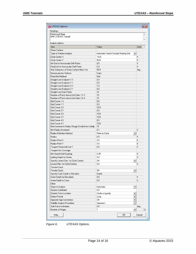
10 Analysis Options

The only thing left to do before saving and running the model is to set the UTEXAS

analysis options. The user will select an automated search for the critical factor of safety

via circular surfaces using Spencer’s Method.

1. In the Project Explorer, right-click on the “UTEXAS” model.

2. Select the Analysis Options command from the pop-up menu.

3. Set Circle Center X to “-10.0.”

4. Set Circle Center Y to “80.0.”

5. Set the Radius Definition Method to “Point on Circle.”

6. Set the Min Search Grid Spacing to “0.25.”

7. Set the Limiting Depth for Circles to “0.0.”

8. The settings should match those shown in the following figure.



Figure 6. UTEXAS Options.



9. When finished, click OK.

At this point, the user should see the starting circle displayed.

11 Save the GMS file

Before continuing, save the GMS project file.

1. Select the File | Save command.

12 Run UTEXAS

Now it is possible to export and run the model in UTEXAS.

12.1 Export the Model

Do the following to export the model:


2. Select the Export command from the pop-up menu.

3. If necessary, locate and open the directory entitled

Tutorials\UTEXAS\reinforcement.

4. Change the File name to “reinforced slope.”

5. Click Save.

12.2 Run UTEXAS

Now that the user has saved the UTEXAS input file, it’s possible to run UTEXAS.


2. Select the Launch UTEXAS4 command from the pop-up menu. This should

bring up the UTEXAS4 program.

3. In UTEXAS4, select the Open File button.

4. Change the Files of type to “All Files (*.*).”

5. Locate the “reinforced slope.utx” file that was just saved (in the

Tutorials\UTEXAS\reinforcement folder).

6. Click Open.



7. Press Save in the Open file for graphics output dialog box. This will save a

TexGraf4 output file.

8. Look at the things mentioned in the Errors, Warnings window, then close the

window.

9. Close the UTEXAS window as well.

12.3 Read the Solution

Now the user needs to read in the UTEXAS solution.


2. Select the Read Solution command from the pop-up menu.

3. Locate the file named “reinforced slope.OUT.”

4. Click Open.

The user should now see a line representing the critical failure surface, and the factor of

safety.

13 Conclusion

This concludes the tutorial. Here are some of the key concepts in this tutorial:

It is possible to use GMS to build reinforced slopes for analysis by UTEXAS.

Reinforcement lines can be placed alone in a separate coverage or included in an

existing coverage.

In GMS, the forces applied along the length of the reinforcement lines are

specified at the nodes.

v. 10 - aquaveogmstutorials-10.0.aquaveo.com/utexas-reinforcedslope.pdf · gms 10.0 tutorial utexas...

Documents