1utdallas.edu/~metin

Planning Demand and Supply in a Supply Chain

Forecasting and Aggregate PlanningChapters 8 and 9

2

utdallas.edu/~metin

Learning Objectives

Overview of forecasting Forecast errors

Aggregate planning in the supply chain Managing demand Managing capacity

3

utdallas.edu/~metin

Phases of Supply Chain Decisions

Strategy or design: Forecast Planning: Forecast Operation/Execution Actual demand

Since actual demands differ from the forecasts, …

so does the execution from the plans. – E.g. Supply Chain degree plans for 40 students per year

whereas the actual is ??

4

utdallas.edu/~metin

Characteristics of forecasts Forecasts are always wrong. Include expected value and measure of error. Long-term forecasts are less accurate than short-term forecasts.

Too long term forecasts are useless: Forecast horizon– Forecasting to determine

» Raw material purchases for the next week; Ericsson» Annual electricity generation capacity in TX for the next 30 years; Texas Utilities » Boat traffic intensity in the upper Mississippi until year 2100; Army Corps of Engineers

Aggregate forecasts are more accurate than disaggregate forecasts– Variance of aggregate is smaller because extremes cancel out

» Two samples: {3,5} and {2,6}. Averages: 4 and 4.

Totals : 8 and 8.» Variance of sample averages/totals=0» Variance of {3,5,2,6}=5/2

– Several ways to aggregate» Products into product groups; Telecom switch boxes» Demand by location; Texas region » Demand by time; April demand

5

utdallas.edu/~metin

Forecasting Methods

Qualitative– Expert opinion

» E.g. Why do you listen to Wall Street stock analysts?

– What if we all listen to the same analyst? S/He becomes right!

Time Series– Static

– Adaptive

Causal: Linear regression Forecast Simulation for planning purposes

9

utdallas.edu/~metin

Master Production Schedule (MPS)

MPS is a schedule of future deliveries. A combination of forecasts and firm orders.

Volume

Time

Firm Orders Forecasts

Frozen Zone Flexible Zone

10utdallas.edu/~metin

Aggregate PlanningChapter 8

11

utdallas.edu/~metin

Aggregate Planning (Ag-gregate: Past part. of Ad-gregare: Totaled)

If the actual is different than the plan, why bother sweating over detailed plans

Aggregate planning: General plan for our frequency decomposition

– Combined products = aggregate product» Short and long sleeve shirts = shirt

Single product

» AC and Heating unit pipes = pipes at Lennox Iowa plant

– Pooled capacities = aggregated capacity» Dedicated machine and general machine = machine

Single capacity– E.g. SOM has 100 instructors

– Time periods = time buckets» Consider all the demand and production of a given month together

When does the demand or production take place in a time bucket? Increase the number of time buckets; decrease the bucket length.

12

utdallas.edu/~metin

Fundamental tradeoffs in Aggregate Planning

Capacity: Regular time, Over time, Subcontract?Inventory: Backlog / lost sales, combination: Customer patience?

Basic Strategies

Chase (the demand) strategy; produce at the instantaneous demand rate

– fast food restaurants

Level strategy; produce at the rate of long run average demand

– swim wear

Time flexibility; high levels of workforce or capacity

– machining shops, army

Deliver late strategy

– spare parts for your Jaguar

13

utdallas.edu/~metin

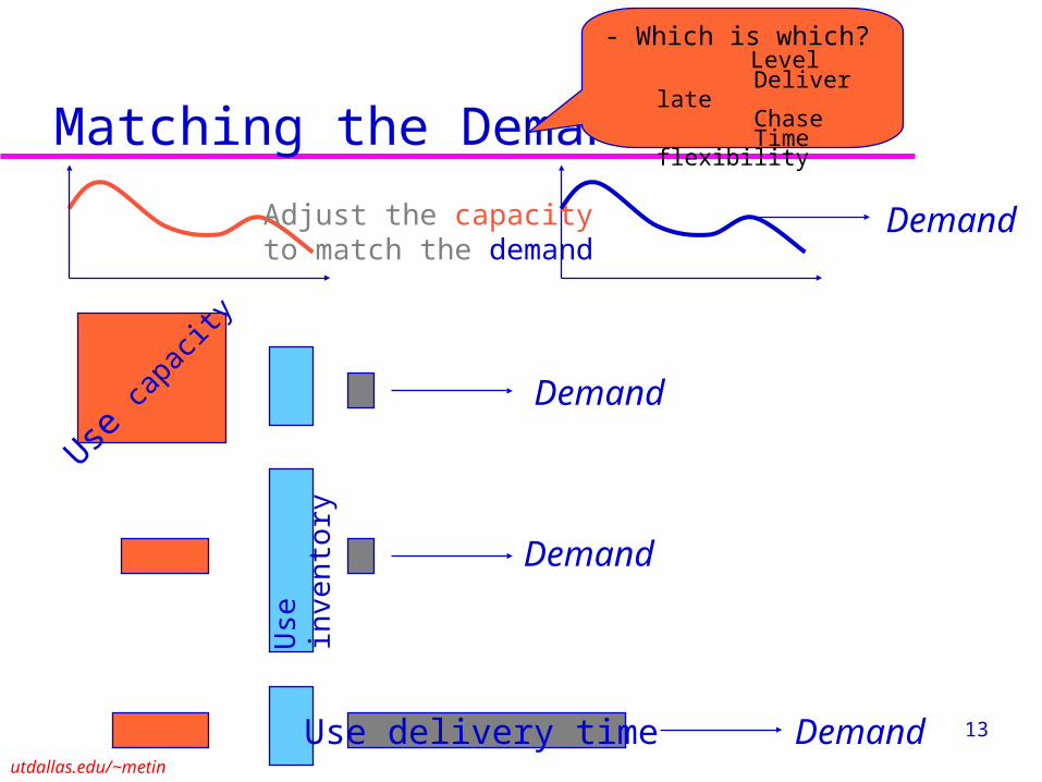
Matching the Demand

Use

inve

ntor

y

Use delivery time

Use ca

pacit

y

Demand

Demand

Demand

Adjust the capacity to match the demand

Demand

- Which is which? Level Deliver late Chase Time flexibility

14

utdallas.edu/~metin

Capacity Demand Matching Inventory/Capacity tradeoff

Level strategy: Leveling capacity forces inventory to build up in anticipation of seasonal variation in demand

Chase strategy: Carrying low levels of inventory requires capacity to vary with seasonal variation in demand or enough capacity to cover peak demand during season

15

utdallas.edu/~metin

Case Study: Aggregate planning at Red Tomato

Farm tools:

Shovels

Spades

Forks

Aggregate by similar characteristics

Generic tool, call it Shovel

Same characteristics?

16

utdallas.edu/~metin

Aggregate Planning at Red Tomato Tools

Month Demand Forecast

January 1,600 February 3,000 March 3,200 April 3,800 May 2,200 June 2,200 Total 16,000

17

utdallas.edu/~metin

Aggregate Planning

Item Cost Materials $10/unit Inventory holding cost $2/unit/month Marginal cost of a backorder $5/unit/month Hiring and training costs $300/worker Layoff cost $500/worker Labor hours required 4hours/unit Regular time cost $4/hour Over time cost $6/hour Max overtime hrs per employee per month 10hours Cost of subcontracting $30/unit Revenue $40/unit

What is the cost of production per tool? That is materials plus labor. Overtime production is more expensive than subcontracting.

What is the saving achieved by producing a tool in house rather than subcontracting?

18

utdallas.edu/~metin

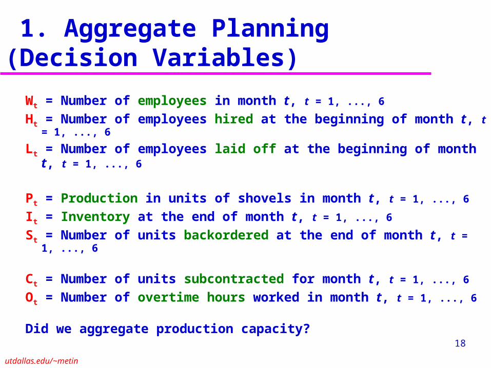
1. Aggregate Planning (Decision Variables)

Wt = Number of employees in month t, t = 1, ..., 6

Ht = Number of employees hired at the beginning of month t, t = 1, ..., 6

Lt = Number of employees laid off at the beginning of month t, t = 1, ..., 6

Pt = Production in units of shovels in month t, t = 1, ..., 6

It = Inventory at the end of month t, t = 1, ..., 6

St = Number of units backordered at the end of month t, t = 1, ..., 6

Ct = Number of units subcontracted for month t, t = 1, ..., 6

Ot = Number of overtime hours worked in month t, t = 1, ..., 6

Did we aggregate production capacity?

19

utdallas.edu/~metin

2. Objective Function:

.80 0 ,6,...,1 01

,1

WwheretforLtH tW tW t

orLtH tW tW t

6

130

6

110

6

15

6

12

6

16

6

1500

6

1300

6

12084

tCt

tPt

tS t

tI t

tOt

tLt

tH t

tW tMin

3. ConstraintsWorkforce size for each month is based on hiring and layoffs

Production (in hours) for each month cannot exceed capacity (in hours)

.6,...,1 ,0440

or 2084

tforPtOtW t

OtW tPt

20

utdallas.edu/~metin

3. Constraints Inventory balance for each month

tP

.500 and 01,000, where1,...,6,for t

0,

,

IS I SISDCPIISDSCPI

600

tt1tttt1t

t1ttttt1t

Periodt

Periodt+1

Periodt-1

1tI tI

tD1tS

tC

tS

21

utdallas.edu/~metin

3. Constraints

Overtime for each month

1,...,6.for t 010

or 10

OWWO

tt

tt

22

utdallas.edu/~metin

Execution

Solve the formulation, see Table 8.3– Total cost=$422.275K, total revenue=$640K

Apply the first month of the plan Delay applying the remaining part of the plan until the next

month Rerun the model with new data next month

This is called rolling horizon execution

23

utdallas.edu/~metin

Aggregate Planning at Red Tomato Tools

Month Demand Forecast January 1,600 February 3,000

March 3,200 April 3,800 May 2,200 June 2,200 Total 16,000

This solution was for the following demand numbers:

What if demand fluctuates more?

24

utdallas.edu/~metin

Increased Demand Fluctuation

Month Demand Forecast January 1,000

February 3,000 March 3,800 April 4,800 May 2,000 June 1,400 Total 16,000

Total costs=$432.858K.16000 units of total production as before why extra cost?

With respect to $422.275K of before.

25utdallas.edu/~metin

Manipulating the DemandChapter 9

26

utdallas.edu/~metin

Matching Demand and Supply

Supply = Demand Supply < Demand => Lost revenue opportunity Supply > Demand => Inventory Manage Supply – Productions Management Manage Demand – Marketing

27

utdallas.edu/~metin

Managing Predictable Variability with SupplyManage capacity

» Time flexibility from workforce (OT and otherwise)» Seasonal workforce, agriculture workers

» Subcontracting

» Counter cyclical products: complementary products Similar products with negatively correlated demands

– Snow blowers and Lawn Mowers

– AC pumps and Heater pumps

» Flexible capacities/processes: Dedicated vs. flexible

a,b,c,d

Similar capabilities One super facility

a

bc

d a

bc

d

28

utdallas.edu/~metin

Managing Predictable Variability with Inventory

Component commonality– Remember fast food restaurant menus

– Component commonality increase the benefit of postponement. » More on this later

Build seasonal inventory of predictable products in preseason– Nothing can be learnt by procrastinating

Keep inventory of predictable products in the downstream supply chain

29

utdallas.edu/~metin

Managing Predictable Variability with PricingRevisit Red Tomato Tools

Manage demand with pricing– Original pricing:

» Cost = $422,275, Revenue = $640,000, Profit=$217,725

Demand increases from discounting– Market growth– Stealing market share from competitors– Forward buying

» stealing your own market share from the future

Discount of $1 in a period increases that period’s demand by 10% (market and market share growth) and moves 20% of next two months demand forward

Can you gather this information –price sensitivity of the demand- easily? Does your company have this information?

30

utdallas.edu/~metin

Off-Peak (January) Discount from $40 to $39

Month Demand Forecast January 3,000=1600(1.1)+0.2(3000+3200) February 2,400=3000(0.8)

March 2,560=3200(0.8) April 3,800 May 2,200 June 2,200

Cost = $421,915, Revenue = $643,400, Profit = $221,485

31

utdallas.edu/~metin

Peak (April) Discount from $40 to $39

Month Demand Forecast January 1,600 February 3,000

March 3,200 April 5,060=3800(1.1)+0.2(2200+2200) May 1,760=2200(0.8) June 1,760=2200(0.8)

Cost = $438,857, Revenue = $650,140, Profit = $211,283Discounting during peak increases the revenue but decreases the profit!

32

utdallas.edu/~metin

Demand Management

Pricing and Aggregate Planning must be done jointly Factors affecting discount timing and their new values

– Consumption: 100% increase in consumption instead of 10% increase

– Forward buy, still 20% of the next two months

– Product Margin: Impact of higher margin. What if discount from $31 to $30 instead of from $40 to $39.)

33

utdallas.edu/~metin

January Discount: 100% increase in consumption, sale price = $40 ($39)

Month Demand Forecast January 4,440=1600(2)+0.2(3000+3200)

February 2,400=0.8(3000) March 2,560=0.8(3200) April 3,800 May 2,200 June 2,200

Off peak discount: Cost = $456,750, Revenue = $699,560Profit=$242,810

34

utdallas.edu/~metin

Peak (April) Discount: 100% increase in consumption, sale price = $40 ($39)

Month Demand Forecast January 1,600 February 3,000 March 3,200 April 8,480=3800(2)+(0.2)(2200+2200) May 1,760=(0.8)2200 June 1,760=(0.8)2200

Peak discount: Cost = $536,200, Revenue = $783,520Profit=$247,320

35

utdallas.edu/~metin

Performance Under Different ScenariosRegular Price

Promotion Price

Promotion Period

% increase in demand

% forward buy

Profit Average Inventory

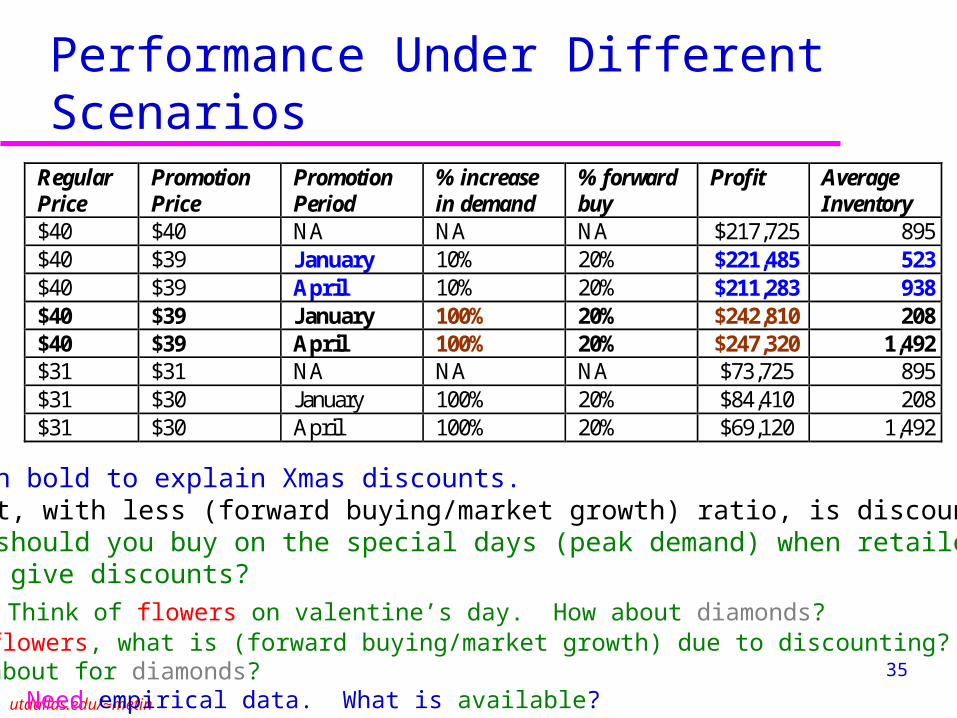
$40 $40 NA NA NA $217,725 895 $40 $39 January 10% 20% $221,485 523 $40 $39 April 10% 20% $211,283 938 $40 $39 January 100% 20% $242,810 208 $40 $39 April 100% 20% $247,320 1,492 $31 $31 NA NA NA $73,725 895 $31 $30 January 100% 20% $84,410 208 $31 $30 April 100% 20% $69,120 1,492 Use rows in bold to explain Xmas discounts. The product, with less (forward buying/market growth) ratio, is discounted more.What gift should you buy on the special days (peak demand) when retailers supposedly give discounts?

E.g. Think of flowers on valentine’s day. How about diamonds?For flowers, what is (forward buying/market growth) due to discounting?How about for diamonds?

Need empirical data. What is available?

36

utdallas.edu/~metin

Empirical Data: Who spends / How much on Valentine’s day

The average consumer spends $122.98 on 2008 Valentine’s Day, similar to $119.67 of 2007. Total US spending on Valentine’s Day is $17.02 B by 18+.

Spending – by gender

» Men again dishes out the most in 2008, spending an average of $163.37 on gifts and cards, compared to an average of $84.72 spent by women.

– by age » Adults: 25-34 spend $160.37.» Young adults: 18-24 spend $145.59.» Upper Middle age: 45-54 spend $117.91. » Lower Middle age: 35-44 spend $116.35.» Elderly: 55-64 spend $110.97.

Gifts» 56.8% of all consumers give a greeting card. » 48.2% plan a special night out. » 48.0% buy candy.» 35.9% buy flowers.» 12.3% give a gift card.» 11.8% buy clothing. » ??.?% buy diamonds

– Source: National Retail Federation www.nrf.com

Where

is forw

ard buy or m

arket

growth

due to disc

ounting?

37

utdallas.edu/~metin

Factors Affecting Promotion Timing

Factor Favored timing High forward buying Low demand period High stealing share High demand period High growth of market High demand period High margin High demand period Low margin Low demand period High holding cost Low demand period Low capacity volume flexibility

Low demand period

38

utdallas.edu/~metin

Aside: Continuous Compounding If my $1investment earns an interest of r per year, what is my

interest+investment at the end of the year? Answer: (1+r) If I earn an interest of r/2 per six months, what is my interest+ investment at the

end of the year? Answer: (1+r/2)2

If I earn an interest of (r/m) per (12/m) months, what is my interest+investment? Answer: (1+r/m)m

Think of continuous compounding as the special case of discrete-time compounding when m approaches infinity.

What if I earn an interest of (r/infinity) per (12/infinity) months?

120

1

24

1

6

1

2

1

1

1

1

11

where1lim :Answer

0

m

n

rm

n!e

em

r

See the appendix of scaggregate.pdf for more on continuous compounding.

39

utdallas.edu/~metin

Deterministic Capacity Expansion Issues Single vs. Multiple Facilities

– Dallas and Atlanta plants of Lockheed Martin Single vs. Multiple Resources

– Machines and workforce; or aggregated capacity Single vs. Multiple Product Demands

– Have you aggregated your demand when studying the capacity? Expansion only or with Contraction

– Is there a second-hand machine market? Discrete vs. Continuous Expansion Times

– Can you expand SOM building capacity during the spring term? Discrete vs. Continuous Capacity Increments

– Can you buy capacity in units of 2.313832? Resource costs, economies of scale Penalty for demand-capacity mismatch

– Recallable capacity: Electricity block outs vs Electricity buy outs» Happens in Wisconsin Electricity market» What if American Airlines recalls my ticket

Single vs. Multiple decision makers

40

utdallas.edu/~metin

A Simple Model

No stock outs. x is the size of the capacity increments.δ is the increase rate of the demand.

D(t)= t

x

Demand

Capacity

Units

Time (t)x/

x

41

utdallas.edu/~metin

Infinite Horizon Total Discounted Cost

f(x) is expansion cost of capacity increment of size x

)/exp(1

)())/(exp()()()(exp)(

00

rx

xfrxxfxf

xkrxC

k

k

k

.1 %;5 ;)( 5.0 rxxf

C(x) is the long run (infinite horizon) total discounted expansion cost

42

utdallas.edu/~metin

Solution of the Simple Model

0

5

10

15

20

25

1 10 20 30 40 50 60 70 80 90 100

Expansion Size

Dis

co

un

ted

Ex

pa

ns

ion

Co

st

Solution can be: Each time expand capacity by an amount that is equal to 30-week demand.

43

utdallas.edu/~metin

Shortages, Inventory Holding, Subcontracting

Use of Inventory and subcontracting to delay capacity expansions

Demand

Units

Time

Capacity

Surpluscapacity

Inventorybuild up

Inventorydepletion

Subcontracting

44

utdallas.edu/~metin

Stochastic Capacity Planning: The case of flexible capacity

Plant 1 and 2 are tooled to produce product A Plant 3 is tooled to produce product B A and B are substitute products

– with random demands DA + DB = Constant

1

2

3

A

B

Plants Products

y1A=1, y2A=1, y3A=0

y1B=0, y2B=0, y3B=1

45

utdallas.edu/~metin

Capacity allocation

Say capacities are r1=r2= r3=100

Suppose that DA + DB = 300 and DA >100 and DB >100

Scenario DA DB X1A X2A X3A X1B X2B X3B Shortage

1 200 100 100 100 100 0

2 150 150 100 50 100 50 B

3 100 200 100 0 100 100 B

With plant flexibility y1A=1, y2A=1, y3A=0, y1B=0, y2B=0, y3B=1.

If the scenarios are equally likely, expected shortage is 50.

46

utdallas.edu/~metin

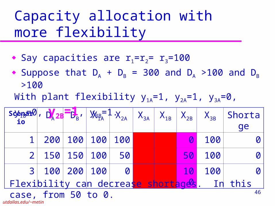
Capacity allocation with more flexibility

Say capacities are r1=r2= r3=100

Suppose that DA + DB = 300 and DA >100 and DB >100

Scenario DA DB X1A X2A X3A X1B X2B X3B Shortage

1 200 100 100 100 0 100 0

2 150 150 100 50 50 100 0

3 100 200 100 0 100 100 0

With plant flexibility y1A=1, y2A=1, y3A=0, y1B=0, y2B=1, y3B=1.

Flexibility can decrease shortages. In this case, from 50 to 0.

47

utdallas.edu/~metin

A Formulation with Known Demands: Dj=dj

i denotes plants j denotes products, not necessarily substitutes

cij tooling cost to configure plant i to produce j

mj contribution to margin of producing/selling a unit of j

ri capacity at plant i Dj=dj product j demand

yij=1 if plant i can produce product j, 0 o.w.

xij=units of j produced at plant i}1,0{y , 0x

dx

rx

rx

Subject to

xm c-Max

ijij

ji

ij

ijiij

jiij

ji,ijjij

ji,ij

jproduct each for

jproduct and iplant each for

iplant each for

y

y

- If DA=200 and DB=100, then y1A=y2A=y3B=1.- If DA=100 and DB=200, then y1A=y2B=y3B=1.

Solutions depend on scenarios:

48

utdallas.edu/~metin

Unknown Demands: Dj=djk with probability pk

Dj=djk product j demand

under scenario k xij

k= units of j produced at plant i if scenario k happens

yij=1 if plant i can produce product j, 0 o.w. Does yij differ under different scenarios?

Should my variable depend on scenarios? (Yes / No)Anticipatory variable and Nonanticapatory variable }1,0{y , 0x

dx

rx

rx

Subject to

xmp c-Max

ijkij

kj

i

kij

ijikij

ji

kij

k ji,

kijj

kij

ji,ij

k scenario and

iproduct each for

k scenario and

jproduct i,plant each for

k scenario and

iplant each for

y

y

49

utdallas.edu/~metin

Reality Check: How do car manufacturers assign products to plants?

With the last formulation, we treated the problem of assigning products to plants.

This type of assignment called for tooling/preparation of each plant appropriately so that it can produce the car type it is assigned to.

These tooling (nonanticipatory) decisions are made at most once a year and manufacturers work with the current assignments to meet the demand.

When market conditions change, the product-to-plant assignment is revisited. – Almost all car manufacturers in North America are retooling their previously truck

manufacturing plants to manufacture compact cars as consumer demand basically disappeared for trucks with high gas prices.

– Also note that the profit margin made from a truck sale is 2-5 times more than the margin made from a car sale. No wonder why manufacturers prefer to sell trucks!

In the following pages, you will find the product to plant assignment of major car manufacturers in the North America. These assignments were updated in the summer of 2008 just about the time when manufacturers started talking about retooling plants to produce compact cars.

50

utdallas.edu/~metin

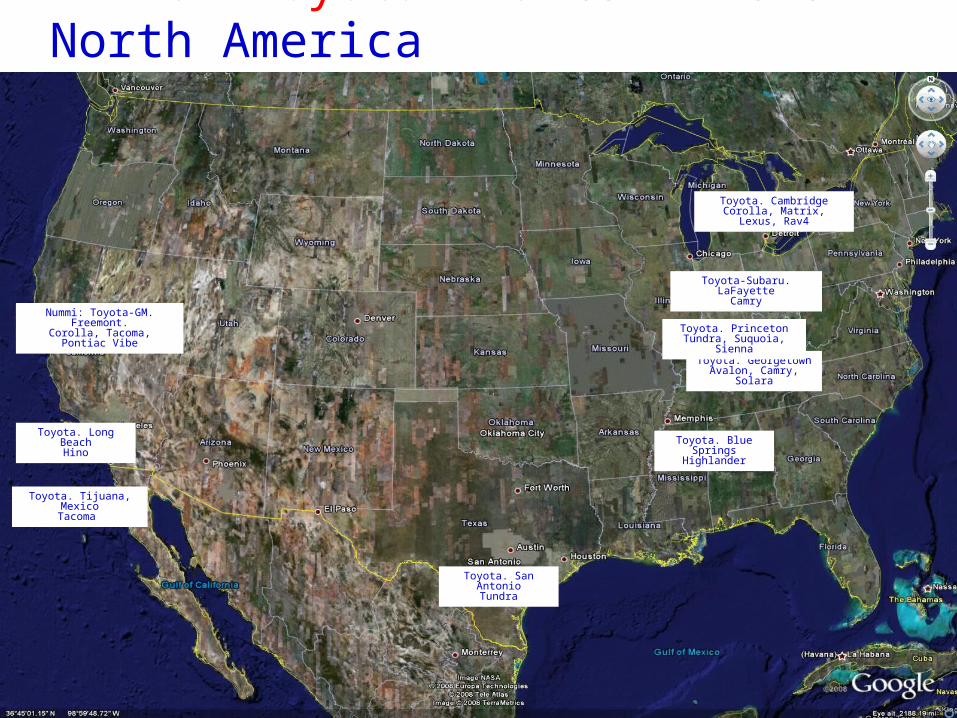
All of Toyota Plants in the North America

Toyota. Tijuana, MexicoTacoma

Toyota. Long BeachHino

Nummi: Toyota-GM. Freemont.Corolla, Tacoma, Pontiac Vibe

Toyota. San AntonioTundra

Toyota. Blue SpringsHighlander

Toyota. GeorgetownAvalon, Camry, Solara

Toyota. PrincetonTundra, Suquoia, Sienna

Toyota-Subaru. LaFayetteCamry

Toyota. CambridgeCorolla, Matrix, Lexus, Rav4

51

utdallas.edu/~metin

All of Honda Plants in the North America

Honda. El Salto, MeAccord

Honda. LincolnOdyssey, Pilot

Honda. MarysvilleAccord, Acura

Honda. DecaturTBO in 2008

Honda. Alliston, Ca.Civic, Acura, Odyssey,

Pilot, Ridgeline

52

utdallas.edu/~metin

All of Nissan Plants in the North America

Nissan. CantonQuest, Armada,

Titan, Infiniti, Altima

Nissan. SmyrnaFrontier, Xterra, Altima,

Maxima, Pathfinder

53

utdallas.edu/~metin

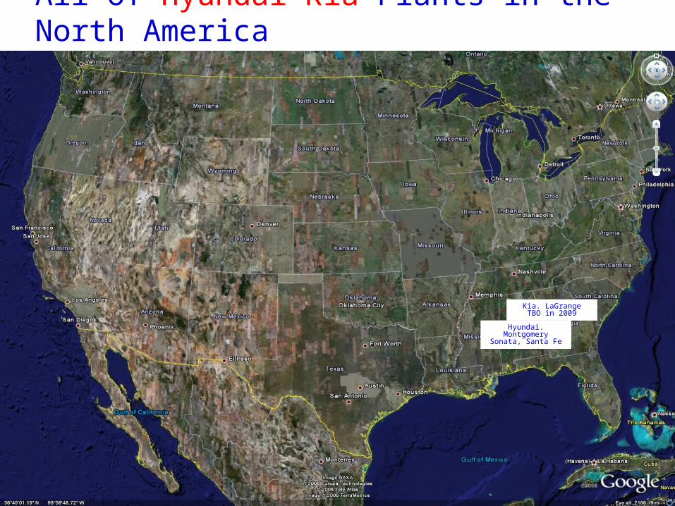
All of Hyundai-Kia Plants in the North America

Hyundai. MontgomerySonata, Santa Fe

Kia. LaGrangeTBO in 2009

54

utdallas.edu/~metin

All of Mercedes and BMW Plants in the North America

Mercedes. TuscaloosaM, R classes

BMW. SpartanburgZ4, X5, X6

M roadster, coupes

55

utdallas.edu/~metin

All of Ford Plants in the North America

Ford. Hermosillo, Mex. Ford Fusion, Lincoln MKZ, Mercury Milan

Ford. Kansas CityEscape, Escape Hybrid,

Mazda Tribute, Mercury Mariner, F-150

Ford. Cuatitlan, Mex. F-150, 250, 350, 450, 550,Ikon

Ford. Saint PaulRanger, Mazda B series

Ford. LouisvilleF-250, F-550, Explorer,Mercury Mountaineer

Ford. ChicagoTaurus, Mercury Sable

Ford. Avon LakeE Series

Ford. Saint Thomas, Ca.Crown Victoria, Grand Marquis

Ford. Oakville, Ca.Edge, Lincoln MKX

Ford. WayneFocus, Expedition, Lincoln Navigator

Ford. Flat RockMustang, Mazda 6

Ford. DearbornF-150, Lincoln Mark LT

Ontario, Michigan, Illinois, Indiana, Ohio in Focus

56

utdallas.edu/~metin

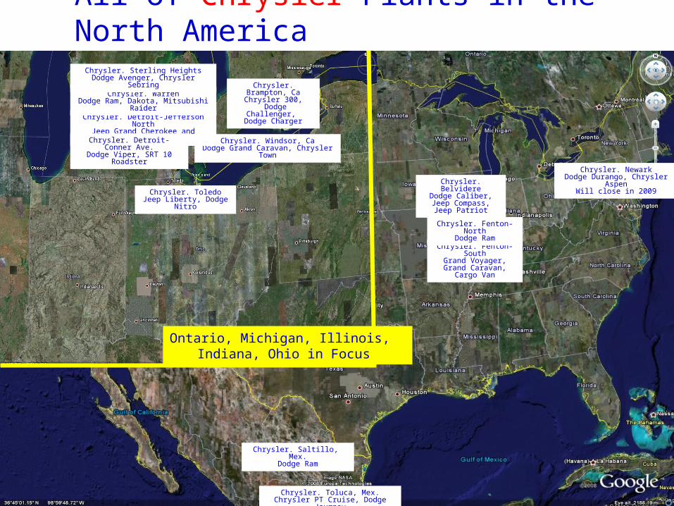
All of Chrysler Plants in the North America

Chrysler. Toluca, Mex.Chrysler PT Cruise, Dodge Journey

Ontario, Michigan, Illinois, Indiana, Ohio in Focus

Chrysler. Saltillo, Mex.Dodge Ram

Chrysler. NewarkDodge Durango, Chrysler Aspen

Will close in 2009

Chrysler. Fenton-SouthGrand Voyager, Grand Caravan, Cargo Van

Chrysler. Fenton-NorthDodge Ram

Chrysler. BelvidereDodge Caliber, Jeep

Compass, Jeep PatriotChrysler. ToledoJeep Liberty, Dodge Nitro

Chrysler. Brampton, CaChrysler 300,

Dodge Challenger, Dodge Charger

Chrysler. Windsor, CaDodge Grand Caravan, Chrysler Town

Chrysler. Detroit-Jefferson NorthJeep Grand Cherokee and Commander

Chrysler. Detroit-Conner Ave.Dodge Viper, SRT 10 Roadster

Chrysler. WarrenDodge Ram, Dakota, Mitsubishi Raider

Chrysler. Sterling HeightsDodge Avenger, Chrysler Sebring

57

utdallas.edu/~metin

All of GM Plants in the North America

GM. Ramos Arizpe, Mex.Pontiac Aztek, Chevy Cavalier, Chevrolet

Checy, Pontiac Sunfire, Buick Rendezvous

Ontario, Michigan, Illinois, Indiana, Ohio in Focus

GM. Silao, Mex.Chevrolet Suburban, Chevrolet Avalanche,

GMC Yukon, Cadillac Escalade

GM. Toluca, Mex.Chevrolet Kodiak Truck

Stopping in 2008

GM. ArlingtonChevy Tahoe,

Suburban, GMC Yukon,

Cadillac Escalade

GM. ShreveportChevy Colorado,

GMC Canyon, Isuzu brands, Hummer H3

GM. FairfaxChevy Malibu, Malibu Maxx, Saturn Aura

GM. WentzvilleChevy Express, GMC Savana

GM. DoravilleChevy Uplander, Pontiac Montana

GM. Spring HillSaturn Ion and Vue

Currently down

GM. Bowling GreenCadillac XLR, Chevy Corvette

GM. WilmingtonSaturn L series, Pontiac Solstice

GM. LordstownChevy Cobalt, Pontiac

Pursuit, G4, G5

GM. MoraineChevy Trailblazer, GMC

Envoy, Oldsmobile Bravada, Isuzu Ascender, Saab 9-7X

Will stop in 2010

GM. Fort WayneChevy Silverado,

GMC Sierra

GM. JanisvilleChevy Tahoe,

Suburban, GMC YukonWill stop in 2010

GM. Oshawa, CaChevy Impala, Buick Allure,

Chevy Silverado, GMC Sierra.Trucks will stop in 2009. GM. Lansing-Grand River

Cadillac E-SRX

GM. Lansing-Delta TownshipBuick Enclave, Saturn Outlook, GMC Acadia

GM. FlintGMC Sierra, Chevy Silverado, Chevy - GMC medium trucks.

GM. PontiacChevy Silverado, GMC Sierra

GM. DetroitBuick Lucerne, Cadillac DTS

GM. OrionPontiac G6,

Chevrolet Malibu

58

utdallas.edu/~metin

Summary of Learning Objectives

Forecasting Aggregate planning Supply and demand management during

aggregate planning with predictable demand variation– Supply management levers

– Demand management levers

Capacity Planning

59

utdallas.edu/~metin

Material Requirements Planning

Master Production Schedule (MPS) Bill of Materials (BOM) MRP explosion Advantages

– Disciplined database– Component commonality

Shortcomings– Rigid lead times– No capacity consideration

60

utdallas.edu/~metin

Optimized Production Technology

Focus on bottleneck resources to simplify planning

Product mix defines the bottleneck(s) ? Provide plenty of non-bottleneck resources. Shifting bottlenecks

61

utdallas.edu/~metin

Just in Time production

Focus on timing Advocates pull system, use Kanban Design improvements encouraged Lower inventories / set up time / cycle time Quality improvements Supplier relations, fewer closer suppliers, Toyota city

JIT philosophically different than OPT or MRP, it is not only a planning tool but a continuous improvement scheme