Computer Science Department

Using Wavelets for Monophonic PitchDetection

John McCulloughHarvey Mudd College

September, 2005

HMC-CS-2005-01

Abstract

Wavelets are an emerging method in the field of signal processing andfrequency estimation. Compared to Fourier and autocorrelation methods,wavelets have a number of advantages. Wavelets based on the derivative ofa smoothing function emphasize points of change in a signal. Positive resultswere achieved when applying such a wavelet to estimate the fundamental fre-quency and corresponding pitch on the equal-temperament harmonic scale.

Keywords: Wavelets, Pitch Detection, Pitch Estimation, Fundamental Fre-quency Estimation

1 Introduction

At the start of the semester I was fascinated with the idea of automatically ex-tracting structural information from music. I had recently seen a presentationon the use of machine learning methods to track individuals in the video fromsecurity cameras to assist in identifying deviant behavior (Jones). The algo-rithms they were using seemed promising and they were making good progressin addressing issues that arose in tracking an object in a scene and, at a sym-bolic level, could do very well. The major issues that exist in computer visioninclude: Identifying objects in the scene, identifying a moving object as thesame between frames, identifying occluding objects within a scene, as well asissues with poor video quality.

During my initial fascination with structure in music, I ignored the issuesassociated with frequency estimation in real signals and superficially thoughtabout the issues of pattern and movement in music at the symbolic level, in amanner similar to the surveillance video. Within machine learning, there aremethods, such as n-grams, that can be applied to sequence prediction althoughnone are able to solve the problem entirely. Then I began to wonder how wemight extract the symbols from a real signal. This, like any type of machineperception, often seems straight-forward at first. We, as humans, are often verygood at it. Unfortunately, transferring our abilities to a machine is very difficult,in part justifying the existence of the machine learning field.

2 Fundamental Frequency Transcription Techniques

A lot of work has been done in the field of musical transcription and com-puter music in general. A variety of methods have been devised to approacha number of them. I hope to address the fundamental ideas of a few that areapplicable to monophonic pitch detection to further my own knowledge and tofacilitate further research. There are several works that cover additional meth-ods in significant detail, (1), and others that focus on more specific methods,(2).

2.1 Fourier

One of the most basic and ubiquitous methods in signal processing is the FourierTransform (FT). It transforms a signal from time space into frequency space.For example, we could decompose a square wave (Figure 1) into its componentparts. There are some assumptions inherent in the way the transform operatesthat are detrimental to identifying frequencies in time: if a frequency is presentin a signal then it is present for the entire duration of that signal and that sig-nal uniformly repeats from −∞ to +∞. The Discrete Fourier Transform (DFT)takes a signal, z, with N samples and calculates the coefficients, Z, correspond-ing to equally spaced frequencies starting with period equal to the length of the

4 2 FUNDAMENTAL FREQUENCY TRANSCRIPTION TECHNIQUES

signal and ending with the sampling frequency, fs:

Z(m) =N∑

n=0

z(n)e(−2πi)(m)(n)

N (1)

where N ∈ Z+ and m,n ∈ {0, 1, 2, . . . , N}. The Z(m) coefficient corresponds tothe frequency (m · fs) (4).

0 0.1 0.2 0.3 0.4 0.5 0.6 0.7 0.8 0.9 1−1

−0.5

0

0.5

1

t (secs)

z(t)

0 5 10 15 20 250

0.5

1

1.5

Hz

Z(m

)

a=0

a=1a=2 a=3 a=4 a=5 a=6 a=7

Summed Square wave

Figure 1: A Square wave is made by the sequence f(t) = sin(2πt) + 13sin(2π3t) +

15sin(2π5t) + 1

2a+1sin(2π(2a + 1)t), a ∈ N. In this example the first seven elements ofthis sum are included (Top). The first twenty-five DFT coefficients of this square waveare also shown (Bottom).

In the example square wave, we can look at the coefficients of the DFT andsee that the appropriate frequencies are in the signal. However, this is onlyeffective when the frequencies are evenly distributed across the signal. If welook at an example that is un-evenly distributed in time and frequency (Figure2), we can see that there are peaks for the the frequency components of thesignal at ±16Hz and ±3Hz, but they are not isolated. The presence of the otherfrequencies in this spectrum are necessary to flatten out the quiet parts. If weconstructed a signal based on these coefficients on the interval 0s to 12s, therewould be two exact repetitions of the signal shown at the top of Figure 2. If welook at the highest peaks we can identify what the fundamental componentsare, though this is not always the case. Because we are in the frequency domain,we cannot identify where in time these frequencies are present based solely onthe spectrum. If we could pick out the frequencies in a signal, it would not dous much good just to know that they existed at some point in a long signal. Itwould be more useful if we looked at shorter sections of a long signal, because

2.1 Fourier 5

using a FT on the shorter sections, we can identify which frequencies exist atthe time and for the duration of each short section.

0 1 2 3 4 5 6−1

−0.5

0

0.5

1

t (secs)

z(t)

−30 −20 −10 0 10 20 300

0.2

0.4

0.6

0.8

Hz

Z

Figure 2: A 16Hz sine wave on the interval 2-3s and a 3Hz sine wave on the interval4-5s (Top). The FT Spectrum (Bottom) of the signal indicates the presence of these twofrequencies as well as a number of others.

The Gabor Transform, also known as the Short Time Fourier Transform(STFT), uses a windowed method. By sliding a window of a given size alongthe signal, we can use the FT to try to identify the frequencies present in eachwindow. The temporal position of each window gives the temporal position ofthe frequencies in that window of the signal. By the nature of the FT, the lengthof the window determines the lowest detectable frequency and is the inverse ofthe window length (Figure 3). A longer window length lowers the detectablefrequency range, but it also lowers the time resolution of the transform (5, 24).Thus, if we want to identify lower frequencies in a signal we reduce our abilityto accurately pick out where any frequency occurs within the signal.

0 0.2 0.4 0.6 0.8 1 1.2 1.4 1.6 1.8 2−1

−0.8

−0.6

−0.4

−0.2

0

0.2

0.4

0.6

0.8

1

t (secs)

f(t)

10Hz Window

10 Hz Period

Figure 3: A sine wave with increasing frequency split into 10Hz windows. A singleperiod of the wave does not fit into the window until the frequency passes above 10Hz.

6 2 FUNDAMENTAL FREQUENCY TRANSCRIPTION TECHNIQUES

2.2 Autocorrelation

Although, for frequency estimation the STFT has many advantages over theregular FT, other methods have also been applied to pitch detection. One suchmethod is autocorrelation, which is achieved by convolving the complex con-jugate1 of a signal with itself. In the continuous case, this can be computed by(1):

Rx(τ) =∫ ∞

−∞x∗(t)x(t + τ)dt (2)

If the R values are computed over the length of the signal and the signal issufficiently self similar, they should exhibit the same fundamental frequency asthe signal (3) (Figure 4). In cases when the signal is not particularly self similarover its entire length (Figure 5) windowing methods can be used, althoughthis can introduce significant computational costs if the windowing function ismore involved than simply analyzing a fixed number of samples (3).

0 0.5 1 1.5 2 2.5 3 3.5 4−3

−2

−1

0

1

2

3

τ, t (secs)

x(t)

, Rx

Autocorrelation Period

Autocorrelation Period

Figure 4: A signal (blue) composed of mixed cosines and the coefficients (red) fromthe autocorrelation values scaled to the range (1,-1). The largest peaks are periodicwith the same frequency as the original signal. The lowest frequencies in the signal aremarked as autocorrelation points for the signal (Above) and the coefficients (Below).

2.3 Wavelets

A.T. Cemgil outlines a number of other methods that can be applied to pitchestimation including FIR and IIR filter banks, which can be viewed as variationson the STFT (1). He also outlined wavelets as a method for signal processing.

Wavelet analysis has fairly diverse and disconnected origins. Morlet, oneoriginator, developed what he called Gabor wavelets using STFT with win-dows of a constant number of oscillations, to look for a particular frequency in

1The complex conjugate is denoted as x∗ and is the negation of the complex component ofa complex number. In Cartesian form ax + bi becomes ax − bi and in polar form aeib becomesae−ib.

2.3 Wavelets 7

0 1 2 3 4 5 6−1

−0.5

0

0.5

1

t (secs)

x(t)

0 0.2 0.4 0.6 0.8 1 1.2 1.4 1.6−1

−0.5

0

0.5

1

τ (secs)

Rx

13Hz 16Hz 3Hz

4Hz

15.9Hz

14.3Hz

Figure 5: A graph of some of the initial autocorrelation Rx values for the mixed 3Hzand 16Hz signal, as in Figure 2, but with a 13Hz sine added on the interval 1.5-1.75s.With the original signal it was possible to find the 3Hz and the 16Hz peaks. However,when the 13Hz portion is introduced the major periodicity in the Rx values is 4Hz (not3Hz) and a 16Hz period is present and no peaks corresponding to 13Hz are visible.

a signal. The window length is determined to be some constant number of pe-riods at that frequency (5). This approach is very similar to what is now knownas the Continuous Wavelet Transform (CWT):

c(a, b) =∫

f(t)Ψ(at + b)dt (3)

The value c(a, b) is the CWT coefficient calculated by convolving the signal,f(t), with a wavelet, Ψ, of scale a at offset b in time. The CWT often refers toa vector of all coefficients for a given scale. The continuous wavelet functionmust have an integral of zero; otherwise the scaling would introduce a bias onthe imbalanced side of the function. Different wavelets at different scales canemphasize different properties in the signal (See Figure 7(a) for a specific exam-ple). A large amount of redundant information is encoded in the CWT becausethe coefficients do not change significantly over small changes in the offset orscale (5). Thus, information is usually extracted solely from the maxima of theCWT coefficients.

When processing large signals or multidimensional signals, calculating theredundant data can make the process computationally infeasible. The FastWavelet Transform (FWT), which was inspired by the pyramid algorithm (5),eliminates redundancy through orthogonality. A pair of functions are orthog-onal if their inner product is zero. This implies that any information encodedby the first wavelet is not encoded by the second and vice-versa; therefore, notime is spent encoding redundant data. The FWT operates using a dyadic scale,

8 3 APPLYING WAVELETS TO PITCH TRANSCRIPTION

progressing in powers of two. These FWT wavelets must satisfy:∫ ∞

−∞Ψ(2it)Ψ(2i+1t)dt = 0, ∀i ≥ 0 (4)

The general idea behind the FWT algorithm is as follows:

A0 ← SignalFor n = 1 until done

Dn ← CWT (An−1, Ψ)An ← Downsample An−1 −Dn by 2

This procedure can continue until a desired level or until there is no addi-tional information to extract. The depth of the algorithm is bounded by n ≤log2(samples) because of the downsampling. To perform noise reduction, itmay only be necessary to compute A1 and then discard D1. The down-samplingreduces the size of the approximation at each level by two. To fully reconstructthe signal, each Ai is needed, along with the final Dn; All intermediate Di maybe discarded. Figure 6 shows a decomposition to n = 5.

Since we have extracted the high frequency information and because of theHeisenberg Uncertainty Principle, no information is lost in the downsampling.The Heisenberg Uncertainty Principle puts a lower bound on the product ∆t ·∆f , which limits the time resolution of lower frequencies (5). There is a morethorough explanation of this behavior in (1).

In practice, both the CWT and down-sampling are performed using specialfilters associated with the wavelet and the associated scaling function, as digitalfilter calculations are much faster than all of the convolutions required for asingle scale of wavelet coefficients. The signal can be reconstructed using thelowest level approximation and the levels of detail above it (Figure 6).

3 Applying Wavelets to Pitch Transcription

3.1 Foundation

A certain type of wavelet is useful for pitch detection with the CWT. Mallatproved that an analysis using a wavelet that is the first derivative of a smooth-ing function will exhibit maxima at points of change in the signal (1). Intu-itively, this makes sense. A smoothing function, such as the gaussian (shownin Figure 7(a)), exhibits the property that, when convolved with a function, willpreserve values closest to a single point in the domain while increasingly de-creasing the values at further points in the domain. As shown in Figure 7(b),the first derivative of a smoothing function will be positive on the left side ofthe center and negative on the right. Thus, a CWT with a wavelet of this shapeemphasizes zero crossings in signals (Figure 8). We can then use the maxima in

3.2 Estimating the Fundamental Frequency 9

200 400 600 800 1000

−5

0

5

a1

−5

0

5

a2

−5

0

5

a3

−5

0

5

a4

−5

0

5

a5

−5

0

5

s

Signal and Approximation(s)

−5

0

5

s

cfs

Coefs, Signal and Detail(s)

54321

−4−2

02

d5

−5

0

5

d4

−202 d

3

−2

0

2d

2

200 400 600 800 1000−2

0

2d

1

(a) An example decomposition from Matlab

etc.

D1

A1

D2

A2

S

(b) A diagram ofthe decomposi-tion.

Figure 6: An example in Matlab of a noisy doppler signal decomposed using a symlet.The s at the top of the right column is the original signal. The decomposition of thesignal is shown from the bottom upward. The s in the right column is the reconstructedsignal, identical to the original, and cfs is a visualization of the coefficients, the scale onthe vertical axis and the offset on the horizontal axis. The coefficients correspond to thecontribution of the 2i scales of wavelets which can be visualized in the detail di. Eachai is the approximation of the signal without the dj ∀j ≤ i.

the coefficients of the CWT to identify zero-crossings in the original signal andcalculate the corresponding frequencies. It is more useful to pick maxima in theCWT coefficients than zero-crossings in the original signal as different scales ofwavelet emphasize different ranges of frequencies, and the original signal oftencontains more frequencies than just the fundamental frequency that we wish toextract.

3.2 Estimating the Fundamental Frequency

Using these wavelet methods I was able to construct a monophonic pitch esti-mator. The general steps in the process are to:

1. Perform the CWT at a single scale, yielding coefficients for each offset.

2. Identify the maxima in the coefficients.

3. Estimate the frequency between each pair of maxima.

10 3 APPLYING WAVELETS TO PITCH TRANSCRIPTION

0 0.1 0.2 0.3 0.4 0.5 0.6 0.7 0.8 0.9 10

0.1

0.2

0.3

0.4

0.5

0.6

0.7

0.8

0.9

1

t (secs)

f(t)

(a) A gaussian with µ = 0.5and σ2 = 0.15

0 0.1 0.2 0.3 0.4 0.5 0.6 0.7 0.8 0.9 1−5

−4

−3

−2

−1

0

1

2

3

4

5x 10

−3

t (secs)

d/dt

f(t)

(b) The first derivative of thegaussian.

Figure 7: The gaussian is an example of a smoothing function whose first derivativecan be used as a wavelet for pitch detection. The quadratic spline is another smoothingfunction that can be used (3).

4. Smooth the frequencies with a running average and clamp them to actualnote frequencies.

5. Group the frequencies into notes with time and duration.

In principle, the analysis should be performed with a wavelet over all of thedyadic scales – because the different scales emphasize different frequencies –and we want to identify notes whose pitches span a wide variety of frequen-cies. Fitch and Shabana (3) suggest that evaluating over three adjacent scaleswas experimentally sufficient to estimate the pitch in the decaying section of aguitar-pluck. In the interest of simplicity and because the papers I read wereopaque on the subject of combining the results from multiple scales, I used asingle scale which was experimentally determined.

After using the first derivative of the gaussian to calculate the coefficients,the maxima are accepted if:

1. they lie above a minimum energy bound which was introduced to suppressthe noise in ‘silent’ areas, and

2. if they are within a certain frequency bound (100Hz to 3000Hz).

The energy of a signal is the squared value of its samples – in this case I am refer-ring to the sum of the squared value of the coefficients between zero-crossings.

Once the maxima in the coefficients are identified, the period between eachadjacent pair is used to compute the frequency at that point in time. In someinstances, when other harmonics or sounds are present, smaller maxima mayappear in between the maxima of the fundamental frequency (6) (Figure 9). Tocompensate for this, the algorithm implements a crude proportion bound: adja-cent maxima are only counted if they are:

3.3 Estimating Pitch 11

0 0.2 0.4 0.6 0.8 1 1.2 1.4 1.6 1.8 2−1

−0.5

0

0.5

1

secs

f(t)

0 0.2 0.4 0.6 0.8 1 1.2 1.4 1.6 1.8 2−1

−0.5

0

0.5

1

secs

f(t)

(a) The wavelet (green) is superim-posed on a 2Hz sine wave offset toalign with a peak of the signal (Top),and to align with a zero-crossing ofthe signal (Bottom).

0 0.2 0.4 0.6 0.8 1 1.2 1.4 1.6 1.8 2−1

−0.8

−0.6

−0.4

−0.2

0

0.2

0.4

0.6

0.8

1

t, offset (secs)

f(t)

, c(t

)

(b) The resulting CWT coefficients(red) scaled to the range (-0.5, 0.5).

Figure 8: A visual example of the CWT using the first derivative of a gaussian asa wavelet. When the wavelet is aligned with a peak in the signal, the positive andnegative portions of the wavelet will cancel, whereas when it is aligned with a zero-crossing in the signal, all portions are positively maximized.

1. within certain proportions of each other or

2. the adjacent maxima are of monatomic ascending or descending magni-tude.i

If those conditions are not met and the next maxima beyond is within the pro-portion bound, it is used to compute the frequency. In an instance when thetwo maxima are farther apart than the period of the minimum frequency, a restfrequency is assigned at the time of both maxima.

3.3 Estimating Pitch

The frequencies are then adjusted to the nearest value on the equal temper-ament harmonic scale. In this scale, developed by Bach, the notes C, C], D,D], E, F, . . . are half steps (multiples of 2

112 ) apart, and the same note one oc-

tave above has twice the frequency (Petersen). After this adjustment, to extractnote start time and duration information, individual time-pitch data-points thathave the same pitch and are adjacent to each other are grouped together. Insome cases, the pitch estimate in a note may deviate for a short period of time.This phenomenon is particularly common in the attack – i.e. the start – of anote as shown in Figure 10. To adjust for this, any note with a duration lessthan a specifiable parameter is merged with the harmonically closest adjacent

12 4 RESULTS

5.73 5.735 5.74 5.745 5.75 5.755 5.760

0.1

0.2

0.3

0.4

0.5

offset (secs)

c

Fundamental F

Smaller Maximum

Unselected due to minimum energy threshold.

tm

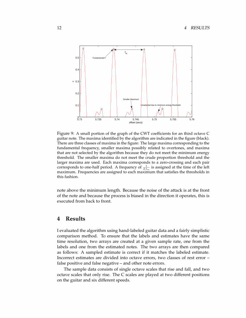
Figure 9: A small portion of the graph of the CWT coefficients for an third octave Cguitar note. The maxima identified by the algorithm are indicated in the figure (black).There are three classes of maxima in the figure: The large maxima corresponding to thefundamental frequency, smaller maxima possibly related to overtones, and maximathat are not selected by the algorithm because they do not meet the minimum energythreshold. The smaller maxima do not meet the crude proportion threshold and thelarger maxima are used. Each maxima corresponds to a zero-crossing and each paircorresponds to one-half period. A frequency of 1

2·tmis assigned at the time of the left

maximum. Frequencies are assigned to each maximum that satisfies the thresholds inthis fashion.

note above the minimum length. Because the noise of the attack is at the frontof the note and because the process is biased in the direction it operates, this isexecuted from back to front.

4 Results

I evaluated the algorithm using hand-labeled guitar data and a fairly simplisticcomparison method. To ensure that the labels and estimates have the sametime resolution, two arrays are created at a given sample rate, one from thelabels and one from the estimated notes. The two arrays are then comparedas follows: A sampled estimate is correct if it matches the labeled estimate.Incorrect estimates are divided into octave errors, two classes of rest error –false positive and false negative – and other note errors.

The sample data consists of single octave scales that rise and fall, and twooctave scales that only rise. The C scales are played at two different positionson the guitar and six different speeds.

13

Nam

eSa

mpl

es%

Cor

rect

%In

corr

ect

%In

cR

est

FP%

Inc

Res

tFN

%In

cN

ote

%In

cO

c-ta

vea3

-a5

2530

097

.64

2.36

15.3

853

.68

0.00

30.9

4b4

-b6

2531

094

.06

5.94

1.33

98.6

70.

000.

00c4

-c5

maj

11

8120

95.3

84.

629.

6057

.87

0.00

32.5

3c4

-c5

maj

12

8219

95.4

64.

5466

.76

33.2

40.

000.

00c4

-c5

maj

21

4365

96.4

03.

6016

.56

83.4

40.

000.

00c4

-c5

maj

22

4533

95.5

24.

4838

.92

61.0

80.

000.

00c4

-c5

maj

31

3515

96.0

53.

9512

.23

87.7

70.

000.

00c4

-c5

maj

32

3011

93.8

26.

1815

.05

84.9

50.

000.

00c4

-c5

maj

41

2601

92.5

87.

429.

8490

.16

0.00

0.00

c4-c

5m

aj4

223

8490

.31

9.69

21.6

567

.10

11.2

60.

00c4

-c5

maj

51

1783

88.2

211

.78

16.6

781

.90

1.43

0.00

c4-c

5m

aj5

217

1588

.28

11.7

28.

4691

.54

0.00

0.00

c4-c

5m

aj6

113

7087

.59

12.4

113

.53

81.7

64.

710.

00c4

-c5

maj

62

1456

83.4

516

.55

45.6

442

.74

11.6

20.

00c5

-c6

maj

181

0098

.80

1.20

25.7

774

.23

0.00

0.00

c5-c

6m

aj2

4170

96.4

33.

5720

.13

75.1

74.

700.

00c5

-c6

maj

329

5095

.32

4.68

0.72

99.2

80.

000.

00c5

-c6

maj

423

6088

.39

11.6

113

.50

82.8

53.

650.

00c5

-c6

maj

518

2093

.41

6.59

5.00

95.0

00.

000.

00c5

-c6

maj

614

4585

.12

14.8

80.

0093

.95

6.05

0.00

d4-d

625

365

98.1

41.

860.

0010

0.00

0.00

0.00

e3-e

525

010

95.1

64.

841.

2498

.76

0.00

0.00

e5-e

725

260

85.3

414

.66

0.05

99.9

50.

000.

00g4

-g6

2540

097

.63

2.37

2.32

97.6

80.

000.

00

Table 1: Performance statistics on guitar data. %Correct and %Incorrect are measuredwith respect to the total number of samples in a comparison performed with a sam-pling frequency of 500Hz. The %Inc values are calculated relative to the number ofincorrect samples. The sample names take the form an-bm-maj s f where a and b arenotes, n and m are octaves, s is the speed (higher is faster), and f is the fret position.

14 4 RESULTS

3.4 3.45 3.5 3.55 3.6 3.65 3.70

20

40

60

80

100

120

140

t (secs)

Hz

(a) Guitar note, sampled at 44.1kHz

0.75 0.8 0.85 0.9 0.95 1 1.05 1.1 1.150

50

100

150

200

250

300

350

400

450

t (secs)

Hz

(b) Violin note, sampled at 22.05kHz

Figure 10: The estimated frequencies (green) after maxima picking – step 3 from 3.2 –at the attack of a guitar note (a) and a violin note (b).

4.1 Error Analysis

In general, the algorithm seems to perform well, as shown in Table 1. The oc-tave errors in the two data-files (a3-a5 and c4-c5 maj 1 1) exhibiting them arerelated to the smaller maxima, potentially related to overtones, in the coeffi-cients (Figure 11). In no instances is an entire note estimated as a different note;the only incidents occur at poorly separated note boundaries (Figure 12). Falsepositives occur primarily at note boundaries. When evaluating the correctnessof the pitch estimates relative to the labeled data, it is important to note that itis unclear whether the hand-labeled “truth” corresponds to precise boundariesin the audio (Figure 13).

Raising the minimum energy threshold can assist in shortening the amountof the decay that is included in the notes’ duration. However, this has a strongeffect of the detection of high frequencies, especially since only a single waveletis being used, which tends to be most selective in a certain range of frequen-cies. At frequencies on the outside of this range, the coefficients tend to bemuch smaller and are therefore more likely to be cut off by the minimum en-ergy threshold (Figure 14). This is exacerbated by the rapid decay of highpitched notes on the guitar. High-frequency errors account for a majority offalse-negative rest errors and there is a strong sensitive dependence amongstthe ability to detect a broad range of frequencies with a single wavelet andthe need to find rests between adjacent notes using only the minimum-energythreshold.

4.2 Conclusions & Future Work 15

9.4 9.6 9.8 10 10.2 10.4 10.6−0.5

0

0.5

1

offset (secs)

C

9.4 9.6 9.8 10 10.2 10.4 10.60

100

200

300

400

secs

Hz

Increasing Proportion

Correct Pitch

Octave Error

Figure 11: An example of an octave error from the a3-a5 scale sample. When the max-ima from the overtones begin to meet the proportionality bound – as illustrated in Figure9 – relative to the maxima corresponding to the fundamental frequency (Top), they areno longer ignored by the algorithm and the estimated frequency approximately dou-bles (Bottom), resulting in octave error. In situations where the octave error is shorterthan the minimum note threshold, the error will be merged into the earlier portion ofthe note at the appropriate pitch. Octave errors occur primarily at the end of notesbecause the amplitude of the fundamental frequency seems to decay faster than theovertones.

4.2 Conclusions & Future Work

Overall I am satisfied with the results of the algorithm as evidenced on this dataset. While there was a small amount of parameter twiddling on the thresholds,it has generally done well. Yet, there is definitely room for improvement, par-ticularly in more dynamic situations with rapid note changes. Currently, onlythe positive maxima are used because the inclusion of the negative maxima in-troduce additional variance in the estimated frequency making it difficult toidentify stable notes. I am uncertain why the negative maxima seem to be lessstable than the positive maxima. Investigating the cause of this, along with thepresence of the lower maxima that induce the octave errors, could be illuminat-ing. Spreading the analysis across multiple scales of wavelet analysis, either asan ensemble classifier or otherwise, should help resolve the issues with high-pitched notes. Such a technique should be particularly effective in correctingoctave errors and possibly reduce the need for identifying low maxima. Thereis potential for improvement in the note grouping algorithm; possibly sometype of predictive look ahead could help relieve the octave error issues. Try-ing to investigate the extra frequencies within the attack of the note, as wellas the frequencies of the harmonics, could help to smooth the pitch estimationand grouping issues. This could also bring some insight into polyphonic pitchtranscription.

16 5 ACKNOWLEDGEMENTS

2.5 2.55 2.6 2.65 2.7 2.750

10

20

30

40

50

60

t (secs)

mid

i not

e

(a) Algorithmically-estimated (cyan •)and hand-labeled (magenta ¤) notesat a note error in c4-c5 maj 6 2.

2.5 2.55 2.6 2.65 2.7 2.75−1

−0.5

0

0.5

1

offset (secs)

C

2.5 2.55 2.6 2.65 2.7 2.75100

150

200

250

300

t (secs)

Hz

estimated frequency

Estimated Notes

(b) The maxima (Top) and calcu-lated frequency with estimated notes(Bottom) for the note error in 12(a).The octave error in the calculatedfrequency is eliminated through thegrouping method.

Figure 12: Note errors primarily occur between two note boundaries than are not wellseparated temporally. Usually this occurs when the attack of the second note overlapswith the decay of the first. The decay as well as other noise in the time between thenotes is not excluded by the minimum energy filter, therefore no rest is detected. Recallthat the grouping algorithm is biased toward the rear, so that the intermediate noiseand noisy sections at the end of the first note are merged in to the second note. Relativeto the algorithm’s pitch estimate, the noisy sections from the first note that are mergedwith the second note are classified as note errors; and the intermediate section is, itself,classified as a false positive rest.

5 Acknowledgements

I would like to thank Professor Belinda Thom for her encouragement, assis-tance, and for letting me research a project completely devoid of the statisticalmethods we’ve been studying in class. I would also like to thank Joseph Walkerfor the use of his labeled guitar data.

17

14.2 14.25 14.3 14.35 14.4 14.45 14.50

20

40

60

t (secs)

mid

i not

e

14.2 14.25 14.3 14.35 14.4 14.45 14.5−0.2

−0.1

0

0.1

0.2

t (secs)

f(t)

(a) Algorithmically-estimated (cyan•)and hand-labeled notes (magenta¤) (Top) and the actual wave data(Bottom) for c4-c5 maj 1 2. Boxesindicate locations where the hand-labeling is questionable.

14.2 14.25 14.3 14.35 14.4 14.45 14.5−1

−0.5

0

0.5

1

1.5

secs

CW

T

14.2 14.25 14.3 14.35 14.4 14.45 14.50

50

100

150

200

secs

Hz

(b) The maxima (Top) and calculatedfrequency with estimated notes (Bot-tom).

Figure 13: Determining the precise boundaries for a note can be difficult, as one mustdetermine where in the attack and in the decay a note begins and ends. Discrepan-cies in the accurate labeling of note boundaries, by hand or otherwise, were generallylinked to rest errors. In general, note boundary issues are categorized as segmentationerrors.

47 47.5 48 48.5 49 49.5 50 50.5 51−0.2

−0.1

0

0.1

0.2

offset (secs)

C

47 47.5 48 48.5 49 49.5 50 50.5 510

200

400

600

800

1000

1200

t (secs)

Hz

Figure 14: An example from b4-b6 where the high-frequency CWT coefficients (Top)are ignored because of the minimum-energy threshold. Near the end of the notes (in-dicated with arrow) the coefficients are very similar in amplitude to the silent portionsof the signal. The initial frequency estimates (Bottom) illustrate which how much ofthe note is missed.

18 REFERENCES

References

[1] Cemgil, A. T. (1995). Automated music transcription.

[2] Evangelista, G. (2001). Flexible wavlets for music signal processing. Journalof New Music Research, 30(1):13–22.

[3] Fitch, J. and Shabana, W. (1999). A wavelet-based pitch detector for mu-sical signals. In Tro, J. and Larsson, M., editors, Proceedings of DAFx99,pages 101–104. Department of Telecommunications, Acoustics Group, Nor-wegian University of Science and Technology. http://www.tele.ntnu.no/akustikk/meetings/DAFx99/fitch.pdf .

[4] Frazier, M. W. (1999). An Introduction to Wavelets Through Linear Algebra.Springer.

[5] Hubbard, B. B. (1998). The World According to Wavelets. A K Peters, secondedition.

[6] Jehan, T. (1997). Music signal parameter estimation. http://web.media.mit.edu/˜tristan/Papers/NVMAT_Tristan.pdf .

[Jones] Jones, G. http://www.kingston.ac.uk/dirc/ .

[Petersen] Petersen, M. Mathematical harmonies. http://amath.colorado.edu/outreach/demos/music/ .