notes wavelets
TRANSCRIPT
7/29/2019 Notes Wavelets
http://slidepdf.com/reader/full/notes-wavelets 1/74
1
4.4.4 Wavelets: Concepts and examples
• What is a wavelet?
A wavelet is a function ( )t ψ of finite energy (L2) whose average is zero:
( ) 0t dt ψ
∞
−∞ =∫ (4.47)
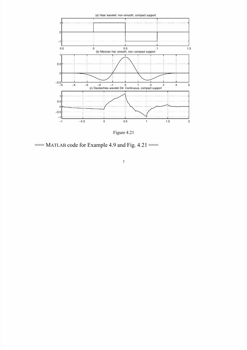
Example 4.9 For the reasons that will become apparent a while later, a useful
wavelet should be a small wave, meaning that it has a compact support , or at least
it approaches zero very quickly as t approaches infinity. However, a wavelet can be either smooth or not so smooth, with or without compact support. See, for
example, the wavelets in Figure 4.21.
7/29/2019 Notes Wavelets
http://slidepdf.com/reader/full/notes-wavelets 2/74
2
−0.5 0 0.5 1 1.5
−1
0
1
(a) Haar wavelet: non−smooth, compact support
−5 −4 −3 −2 −1 0 1 2 3 4 5−0.5
0
0.5
1(b) Mexican hat: smooth, non−compact support
−1 −0.5 0 0.5 1 1.5 2
−1
−0.5
0
0.5
1
(c) Daubechies wavelet D4: Continuous, compact support
Figure 4.21
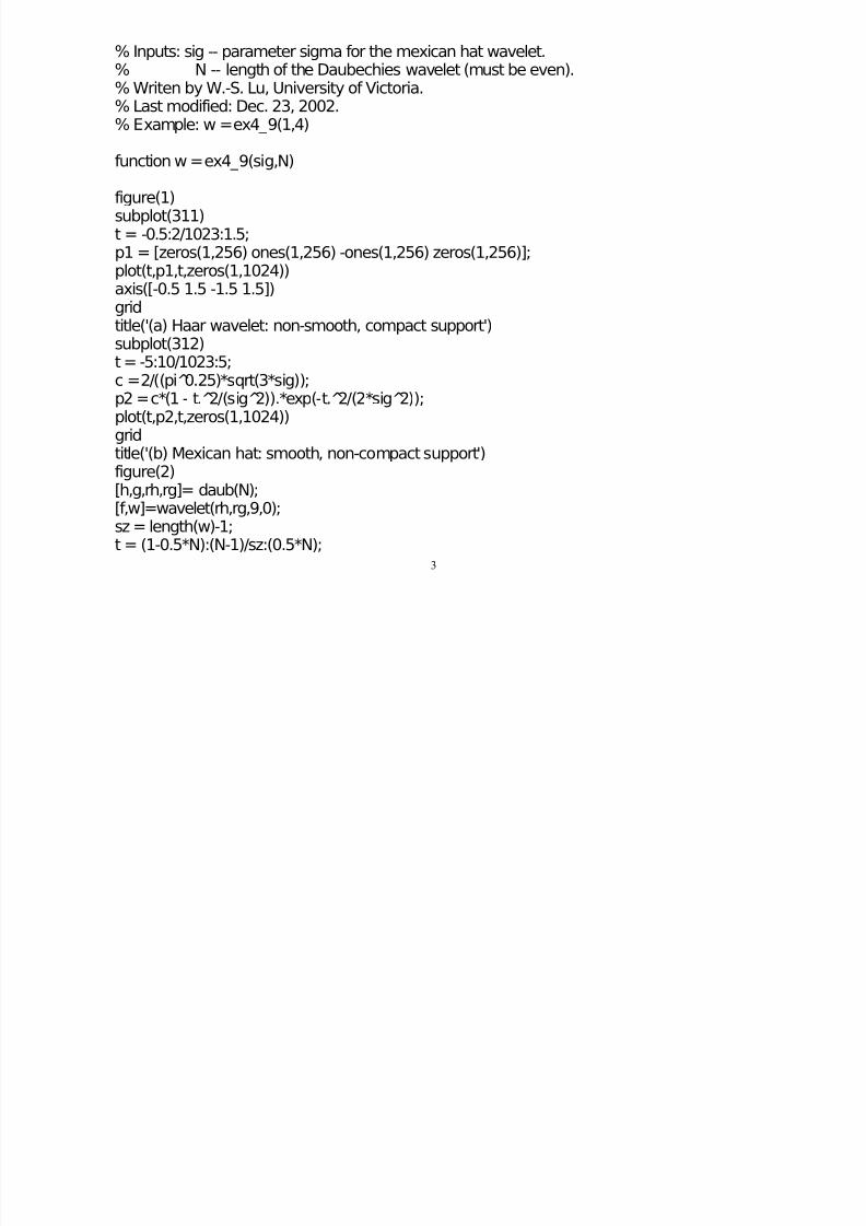
=== MATLAB code for Example 4.9 and Fig. 4.21 ===
7/29/2019 Notes Wavelets
http://slidepdf.com/reader/full/notes-wavelets 3/74
3
% Inputs: sig -- parameter sigma for the mexican hat wavelet.% N -- length of the Daubechies wavelet (must be even).% Writen by W.-S. Lu, University of Victoria.
% Last modified: Dec. 23, 2002.% Example: w = ex4_9(1,4)
function w = ex4_9(sig,N)
figure(1)
subplot(311)t = -0.5:2/1023:1.5;p1 = [zeros(1,256) ones(1,256) -ones(1,256) zeros(1,256)];plot(t,p1,t,zeros(1,1024))axis([-0.5 1.5 -1.5 1.5])gridtitle('(a) Haar wavelet: non-smooth, compact support')subplot(312)t = -5:10/1023:5;c = 2/((pi 0̂.25)*sqrt(3*sig));p2 = c*(1 - t. 2̂/(sig 2̂)).*exp(-t. 2̂/(2*sig 2̂));plot(t,p2,t,zeros(1,1024))gridtitle('(b) Mexican hat: smooth, non-compact support')figure(2)[h,g,rh,rg]= daub(N);[f,w]=wavelet(rh,rg,9,0);
sz = length(w)-1;t = (1-0.5*N):(N-1)/sz:(0.5*N);
7/29/2019 Notes Wavelets
http://slidepdf.com/reader/full/notes-wavelets 4/74
4
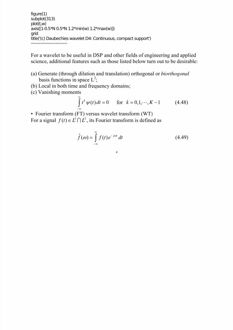
figure(1)subplot(313)plot(t,w)
axis([1-0.5*N 0.5*N 1.2*min(w) 1.2*max(w)])gridtitle('(c) Daubechies wavelet D4: Continuous, compact support')===============
For a wavelet to be useful in DSP and other fields of engineering and appliedscience, additional features such as those listed below turn out to be desirable:
(a) Generate (through dilation and translation) orthogonal or biorthogonal
basis functions in space L2;
(b) Local in both time and frequency domains;(c) Vanishing moments
( ) 0 for 0,1, , 1k t t dt k K ψ
∞
−∞
= = −∫ (4.48)
• Fourier transform (FT) versus wavelet transform (WT)For a signal
1 2( ) f t L L∈ ∩ , its Fourier transform is defined as
ˆ ( ) ( ) j t f f t e dt
ω ω ∞
−
−∞
= ∫ (4.49)
7/29/2019 Notes Wavelets
http://slidepdf.com/reader/full/notes-wavelets 5/74
5
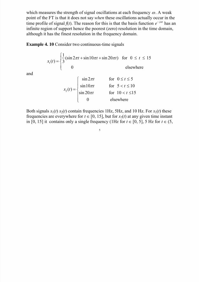
which measures the strength of signal oscillations at each frequency ω . A weak
point of the FT is that it does not say when these oscillations actually occur in the
time profile of signal f (t ). The reason for this is that the basis function j t
e
ω −
has aninfinite region of support hence the poorest (zero) resolution in the time domain,
although it has the finest resolution in the frequency domain.
Example 4. 10 Consider two continuous-time signals
1
1(sin 2 sin10 sin 20 ) for 0 15
( ) 3
0 elsewhere
t t t t x t
π π π ⎧
+ + ≤ ≤⎪= ⎨
⎪⎩
and
2
sin 2 for 0 5
sin10 for 5 10( )
sin 20 for 10 15
0 elsewhere
t t
t t x t
t t
π
π
π
≤ ≤⎧⎪ < ≤⎪
= ⎨< ≤⎪
⎪⎩
Both signals x1(t ) x2(t ) contain frequencies 1Hz, 5Hz, and 10 Hz. For x1(t ) these
frequencies are everywhere for t ∈ [0, 15], but for x2(t ) at any given time instant
in [0, 15] it contains only a single frequency (1Hz for t ∈ [0, 5], 5 Hz for t ∈ (5,
7/29/2019 Notes Wavelets
http://slidepdf.com/reader/full/notes-wavelets 6/74
6
10], and 10 Hz for t ∈ (10, 15]).
To get the spectrum of the signals, we sample them for t ∈ [0, 15] with rate f s = 40Hz, yielding 601 samples for each of the signals denoted by x1[n] and x2[n]
respectively, and perform DFT of the discrete-time signals obtained.
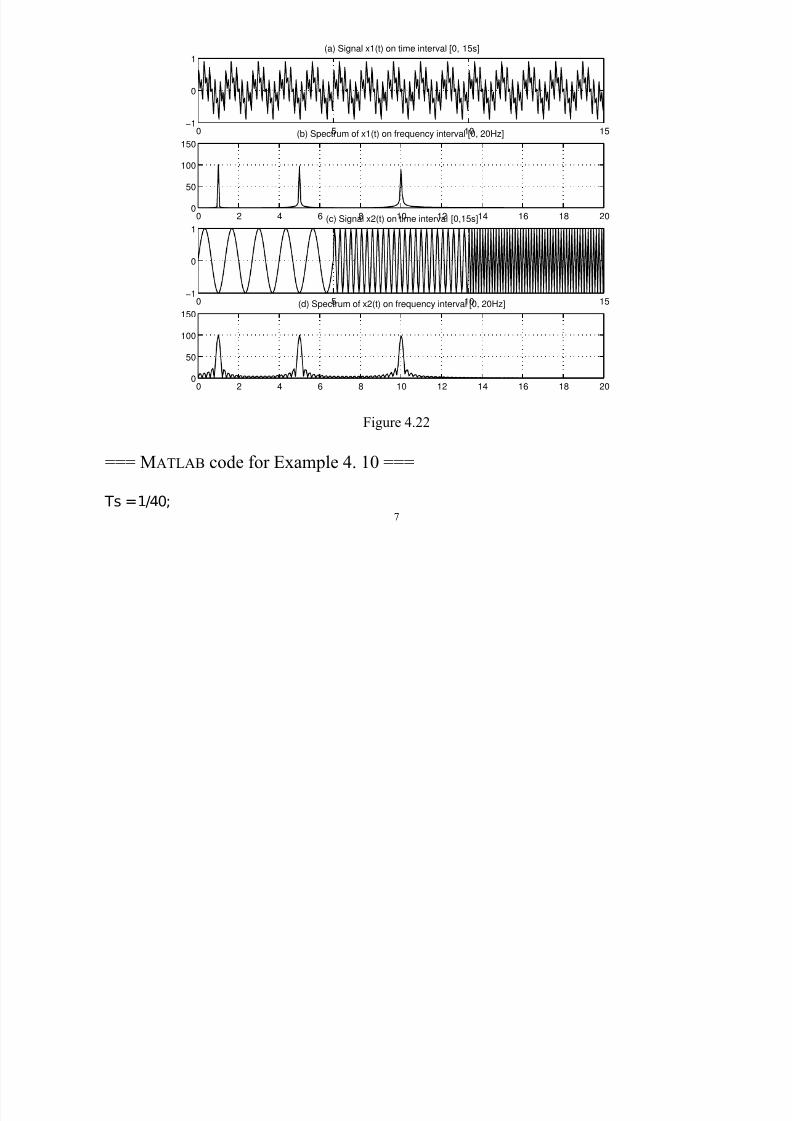
The signals x1(t ) and x2(t ) as well as their spectra are shown in Fig. 4.22. It is
observed that although the time-domain profiles of the signals are quite different,their spectra are similar to each other. In other words, the spectrum provides no
immediate and explicit information as which part(s) of the signal’s time-domain
profile have contributed to the signal’s spectrum strength at a specified frequency.
7/29/2019 Notes Wavelets
http://slidepdf.com/reader/full/notes-wavelets 7/74
7
0 5 10 15−1
0
1(a) Signal x1(t) on time interval [0, 15s]
0 2 4 6 8 10 12 14 16 18 200
50
100
150(b) Spectrum of x1(t) on frequency interval [0, 20Hz]
0 5 10 15−1
0
1(c) Signal x2(t) on time interval [0,15s]
0 2 4 6 8 10 12 14 16 18 20
0
50
100
150(d) Spectrum of x2(t) on frequency interval [0, 20Hz]
Figure 4.22
=== MATLAB code for Example 4. 10 ===
Ts = 1/40;
7/29/2019 Notes Wavelets
http://slidepdf.com/reader/full/notes-wavelets 8/74
8
t1 = 0:Ts:5;t2 = (5+Ts):Ts:10;t3 = (10+Ts):Ts:15;
t = [t1 t2 t3];x1 = (sin(2*pi*t)+sin(10*pi*t)+sin(20*pi*t))/3;x21 = sin(2*pi*t1);x22 = sin(10*pi*t2);x23 = sin(20*pi*t3);x2 = [x21 x22 x23];
xf1=fft(x1);xf2=fft(x2);fs = 1/Ts;L = (length(x1)-1)/2;f=0:(fs/2)/L:(fs/2);figure(1)
subplot(411)plot(t,x1)gridtitle('(a) Signal x1(t) on time interval [0, 15s]')subplot(412)plot(f,abs(xf1(1:L+1)))gridtitle('(b) Spectrum of x1(t) on frequency interval [0, 20Hz] ')subplot(413)plot(t,x2)grid
title('(c) Signal x2(t) on time interval [0,15s]')subplot(414)
7/29/2019 Notes Wavelets
http://slidepdf.com/reader/full/notes-wavelets 9/74
9
plot(f,abs(xf2(1:L+1)))gridtitle('(d) Spectrum of x2(t) on frequency interval [0, 20Hz]')
==========
♦ Remark: At another extreme of the spectrum, we note that Dirac’s delta
function, which has also been popular in signal analysis, has the finest resolution
in the time domain but the poorest resolution in the frequency domain.
Now suppose we have a wavelet function 2( )t Lψ ∈ which satisfies (4.47) and
( ) 1t ψ = . The wavelet transform of f (t ) at time u and scale s is defined as
1
( , ) ( ) ( )
t u f u s f t dt
ss ψ
∞
−∞
−=
∫
(4.50)
From (4.50) we see that a WT of signal f (t ) defines a family of functions rather
than a single function:
For each fixed scale (resolution) s, the WT in (4.50) can be viewed as a linear
filtering process with a filter whose impulse response is given by
1
( ) ( )s
t t
ssψ ψ
−=
(4.51)
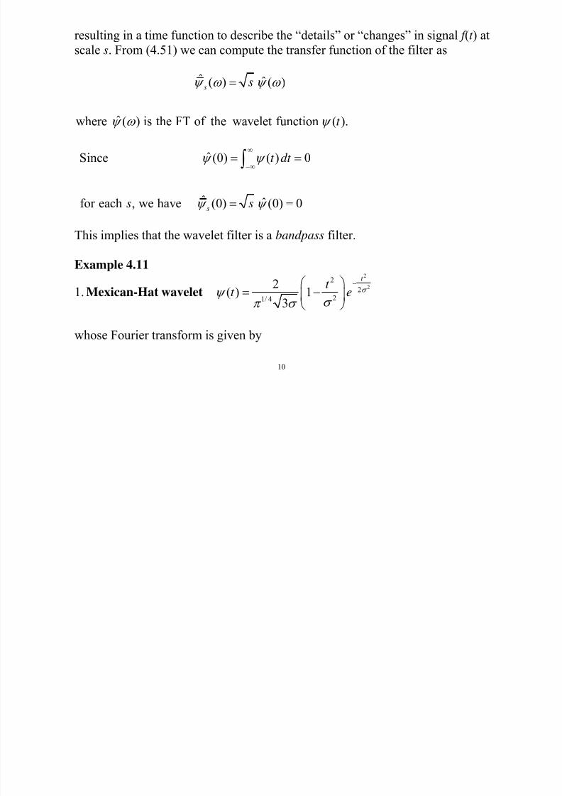
7/29/2019 Notes Wavelets
http://slidepdf.com/reader/full/notes-wavelets 10/74
10
resulting in a time function to describe the “details” or “changes” in signal f (t ) at
scale s. From (4.51) we can compute the transfer function of the filter as
ˆ ˆ( ) ( )
ˆwhere ( ) is the FT of the wavelet function ( ).
ss
t
ψ ω ψ ω
ψ ω ψ
=
ˆSince (0) ( ) 0
ˆˆfor each , we have (0) (0) 0s
t dt
s s
ψ ψ
ψ ψ
∞
−∞= =
= =
∫
This implies that the wavelet filter is a bandpass filter.
Example 4.11
1. Mexican-Hat wavelet2
22
221/ 4
2( ) 1
3
t t t e σ ψ
σ π σ
−⎛ ⎞= −⎜ ⎟⎝ ⎠
whose Fourier transform is given by

7/29/2019 Notes Wavelets
http://slidepdf.com/reader/full/notes-wavelets 11/74
11
2 25/ 2 1/ 4
2 / 28ˆ ( )
3e
σ ω σ π ψ ω ω −=
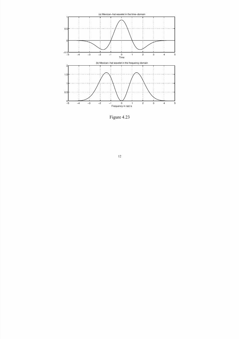
The plots of the Mexican hat wavelet (with σ = 1) and its FT are shown in Fig.
4.23. We observe that
♦ ( )t ψ is smooth. It has an infinite support but most of its energy is concentrated
in a rather small region in the time domain.
♦ ˆ ( )ψ ω is bandpass with its largest gain at 1.42 rad./s.
♦ ˆ ( )ψ ω has an infinite support as well, but its energy is concentrated in a small
region in the frequency domain.
7/29/2019 Notes Wavelets
http://slidepdf.com/reader/full/notes-wavelets 12/74
12
−5 −4 −3 −2 −1 0 1 2 3 4 5−0.5
0
0.5
1(a) Mexican−hat wavelet in the time−domain
Time
−5 −4 −3 −2 −1 0 1 2 3 4 50
0.5
1
1.5
2(b) Mexican−hat wavelet in the frequency domain
Frequency in rad./s
Figure 4.23
7/29/2019 Notes Wavelets
http://slidepdf.com/reader/full/notes-wavelets 13/74
13
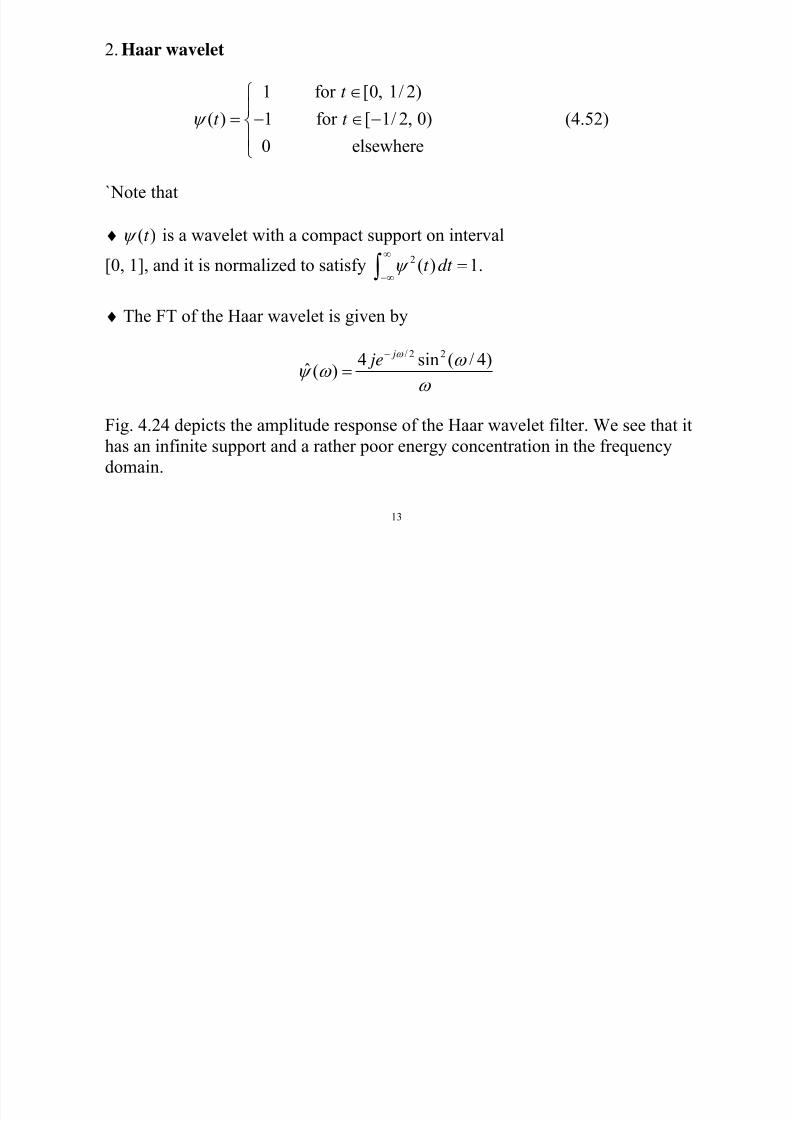
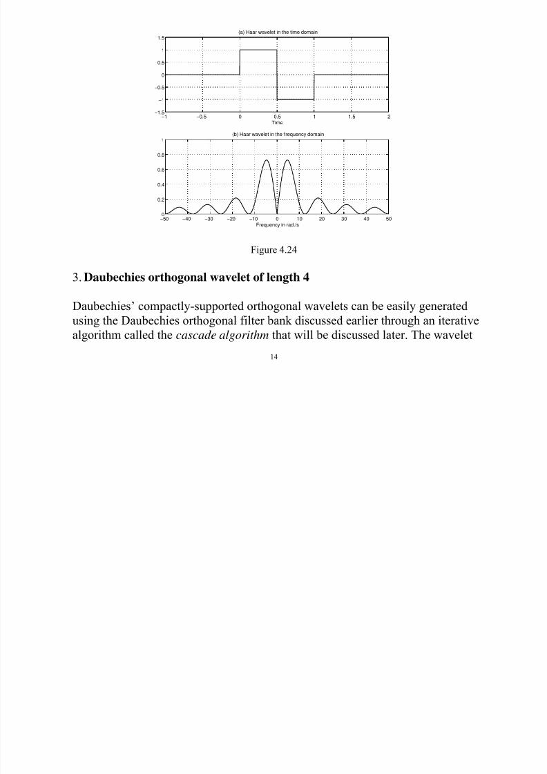
2. Haar wavelet
1 for [0, 1/ 2)( ) 1 for [ 1/ 2, 0)
0 elsewhere
t t t ψ
∈⎧⎪= − ∈ −⎨⎪⎩
(4.52)
`Note that
♦ ( )t ψ is a wavelet with a compact support on interval
[0, 1], and it is normalized to satisfy 2 ( ) 1t dt ψ ∞
−∞=∫ .
♦ The FT of the Haar wavelet is given by
/ 2 24 sin ( / 4)ˆ ( )
j je
ω ω
ψ ω
ω
−
=
Fig. 4.24 depicts the amplitude response of the Haar wavelet filter. We see that it
has an infinite support and a rather poor energy concentration in the frequency
domain.
7/29/2019 Notes Wavelets
http://slidepdf.com/reader/full/notes-wavelets 14/74
14
−1 −0.5 0 0.5 1 1.5 2−1.5
−1
−0.5
0
0.5
1
1.5(a) Haar wavelet in the time domain
Time
−50 −40 −30 −20 −10 0 10 20 30 40 500
0.2
0.4
0.6
0.8
1 (b) Haar wavelet in the frequency domain
Frequency in rad./s
Figure 4.24
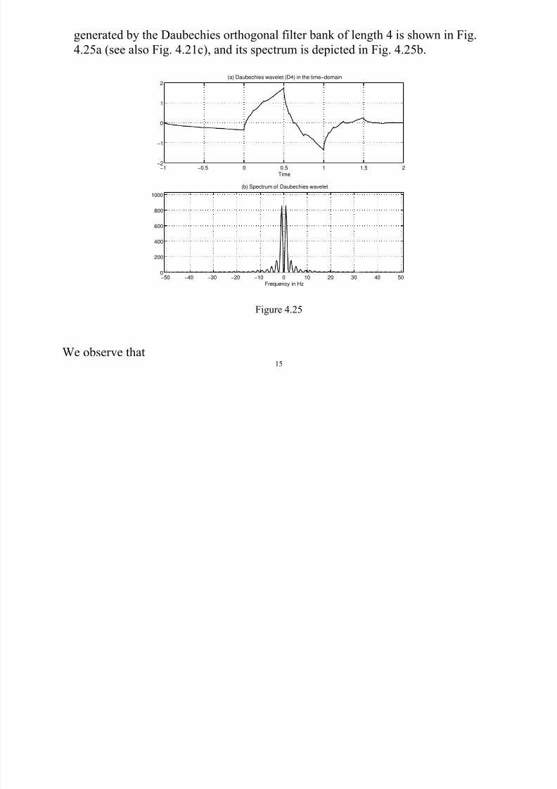
3. Daubechies orthogonal wavelet of length 4
Daubechies’ compactly-supported orthogonal wavelets can be easily generated
using the Daubechies orthogonal filter bank discussed earlier through an iterative
algorithm called the cascade algorithm that will be discussed later. The wavelet
7/29/2019 Notes Wavelets
http://slidepdf.com/reader/full/notes-wavelets 15/74
15
generated by the Daubechies orthogonal filter bank of length 4 is shown in Fig.
4.25a (see also Fig. 4.21c), and its spectrum is depicted in Fig. 4.25b.
−1 −0.5 0 0.5 1 1.5 2−2
−1
0
1
2(a) Daubechies wavelet (D4) in the time−domain
Time
−50 −40 −30 −20 −10 0 10 20 30 40 500
200
400
600
800
1000
(b) Spectrum of Daubechies wavelet
Frequency in Hz
Figure 4.25
We observe that
7/29/2019 Notes Wavelets
http://slidepdf.com/reader/full/notes-wavelets 16/74
16
♦ Although not very smooth, the Daubechies wavelet is continuous, and has a
finite region of support.♦ ˆ ( )ψ ω is bandpass.
♦ ˆ ( )ψ ω has an infinite support, but its energy is concentrated in a small region
relative to that of the Haar wavelet. ■
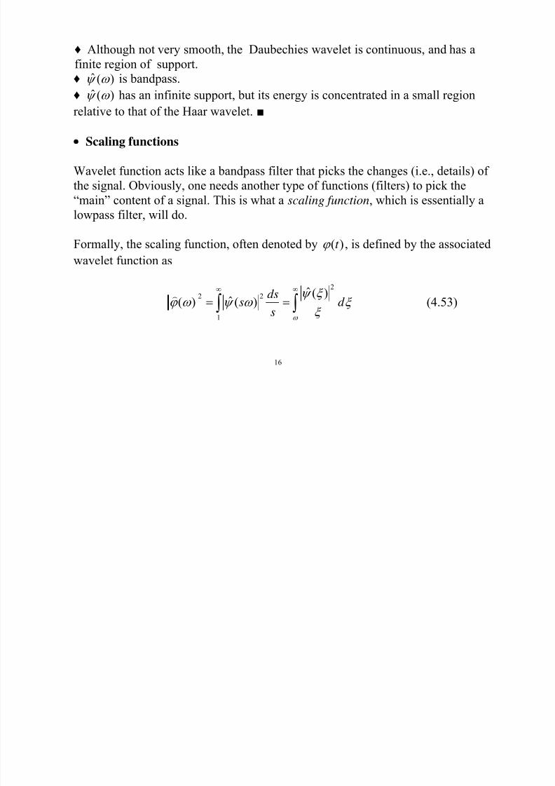
• Scaling functions
Wavelet function acts like a bandpass filter that picks the changes (i.e., details) of
the signal. Obviously, one needs another type of functions (filters) to pick the
“main” content of a signal. This is what a scaling function, which is essentially a
lowpass filter, will do.
Formally, the scaling function, often denoted by ( )t ϕ , is defined by the associated
wavelet function as
2
2 2
1
ˆ ( )ˆ( ) ( )
dss d
sω
ψ ξ ϕ ω ψ ω ξ
ξ
∞ ∞
= =∫ ∫
(4.53)
7/29/2019 Notes Wavelets
http://slidepdf.com/reader/full/notes-wavelets 17/74
17
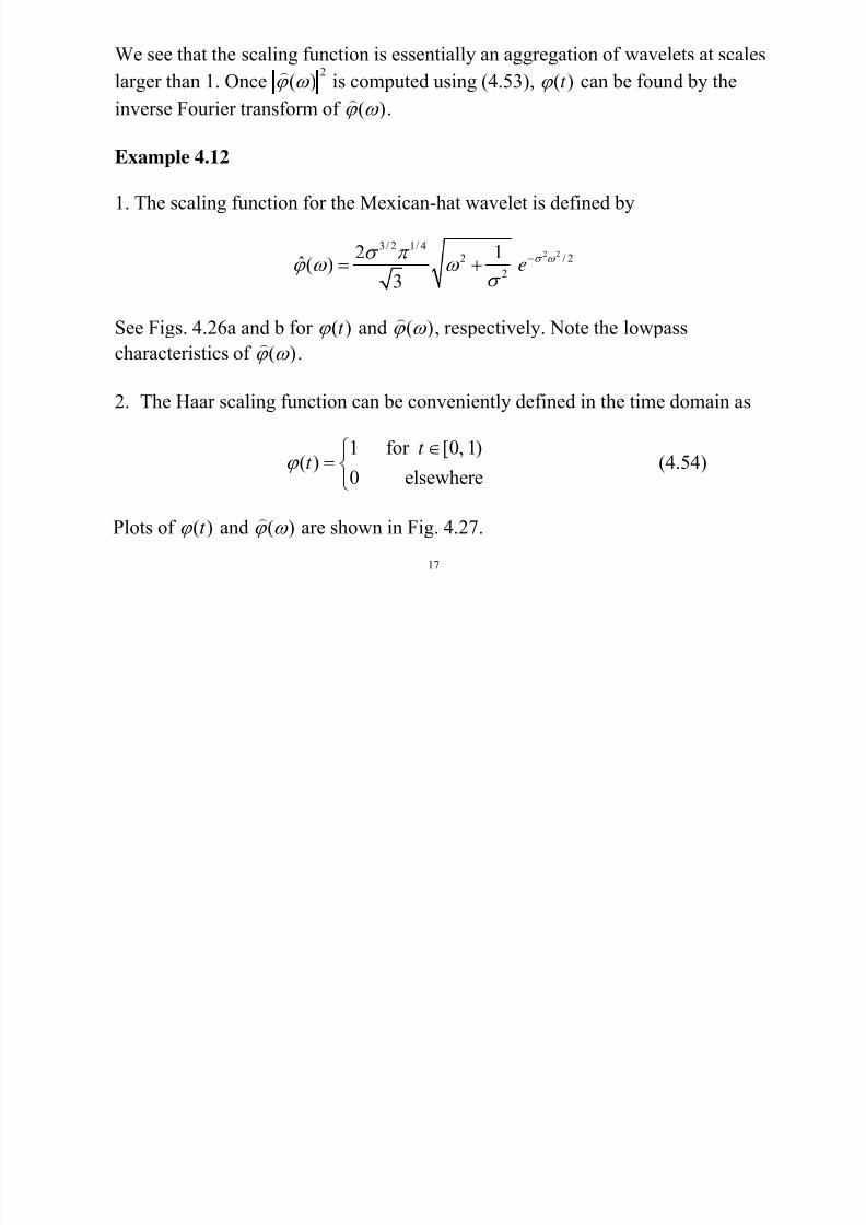
We see that the scaling function is essentially an aggregation of wavelets at scales
larger than 1. Once2
( )ϕ ω
is computed using (4.53), ( )t ϕ can be found by the
inverse Fourier transform of ( )ϕ ω
.
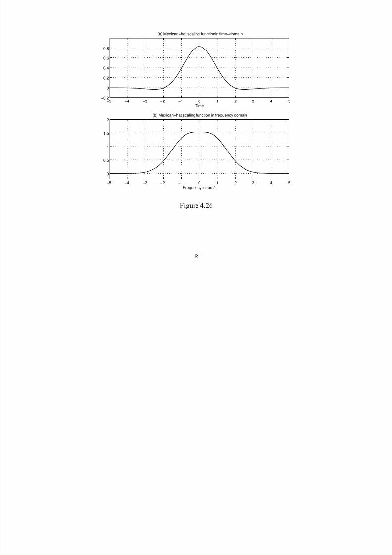
Example 4.12
1. The scaling function for the Mexican-hat wavelet is defined by
2 23/ 2 1/ 4
2 / 2
2
2 1ˆ( )
3e
σ ω σ π ϕ ω ω
σ
−= +
See Figs. 4.26a and b for ( )t ϕ and ( )ϕ ω , respectively. Note the lowpasscharacteristics of ( )ϕ ω
.
2. The Haar scaling function can be conveniently defined in the time domain as
1 for [0, 1)( )
0 elsewhere
t t ϕ
∈⎧= ⎨
⎩(4.54)
Plots of ( )t ϕ and ( )ϕ ω
are shown in Fig. 4.27.
7/29/2019 Notes Wavelets
http://slidepdf.com/reader/full/notes-wavelets 18/74
18
−5 −4 −3 −2 −1 0 1 2 3 4 5
0
0.5
1
1.5
2(b) Mexican−hat scaling function in frequency domain
Frequency in rad./s
−5 −4 −3 −2 −1 0 1 2 3 4 5−0.2
0
0.2
0.4
0.6
0.8
(a) Mexican−hat scaling functionin time−domain
Time
Figure 4.26
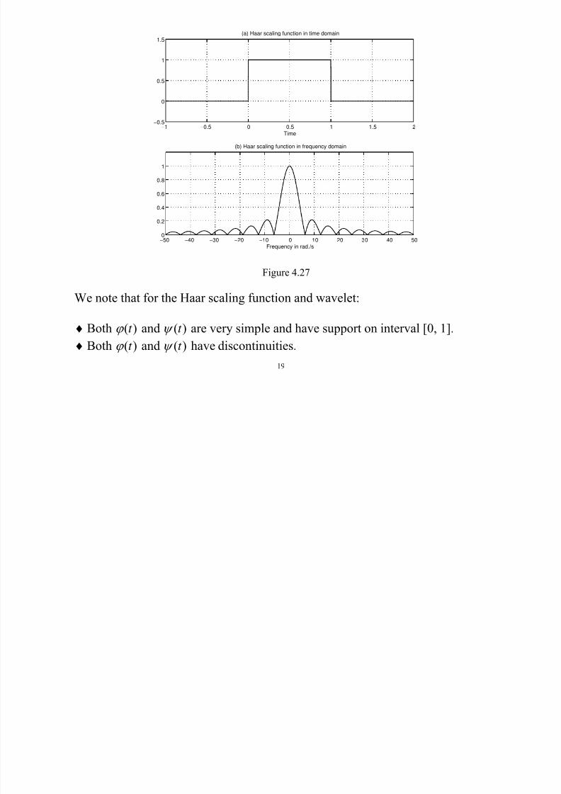
7/29/2019 Notes Wavelets
http://slidepdf.com/reader/full/notes-wavelets 19/74
19
−1 −0.5 0 0.5 1 1.5 2−0.5
0
0.5
1
1.5(a) Haar scaling function in time domain
Time
−50 −40 −30 −20 −10 0 10 20 30 40 500
0.2
0.4
0.6
0.8
1
(b) Haar scaling function in frequency domain
Frequency in rad./s
Figure 4.27
We note that for the Haar scaling function and wavelet:
♦ Both ( )t ϕ and ( )t ψ are very simple and have support on interval [0, 1].
♦ Both ( )t ϕ and ( )t ψ have discontinuities.

7/29/2019 Notes Wavelets
http://slidepdf.com/reader/full/notes-wavelets 20/74
20
♦ Both ( ) and ( )ϕ ω ψ ω
are continuous and somewhat local.
♦ ( )ϕ ω
exhibits a lowpass characteristic.
1. The Daubechies scaling function associated with Daubechies orthogonal filter
bank of length N can also be generated using the cascade algorithm. The
scaling function has a compact (i.e. finite) region of support on the time
interval [0, N – 1]. Figs 4.28a and b depict the scaling function with N = 4 and
its spectrum, respectively.

7/29/2019 Notes Wavelets
http://slidepdf.com/reader/full/notes-wavelets 21/74
21
0 0.5 1 1.5 2 2.5 3−2
−1
0
1
2(a) Daubechies scaling function (N = 4) in time−domain
Time
−50 −40 −30 −20 −10 0 10 20 30 40 500
200
400
600
800
1000
1200
(b) Spectrum of Daubechies scaling funtion (N = 4)
Frequency in Hz
Figure 4.28
7/29/2019 Notes Wavelets
http://slidepdf.com/reader/full/notes-wavelets 22/74
22
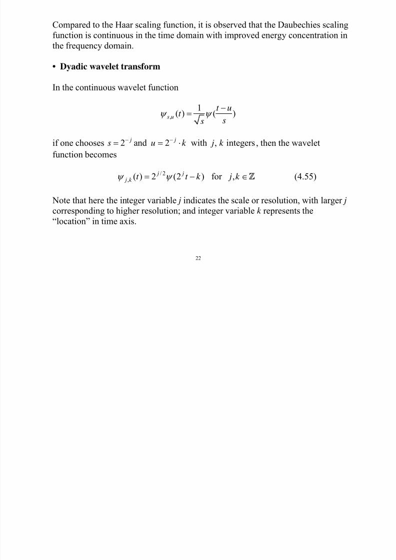
Compared to the Haar scaling function, it is observed that the Daubechies scaling
function is continuous in the time domain with improved energy concentration in
the frequency domain.
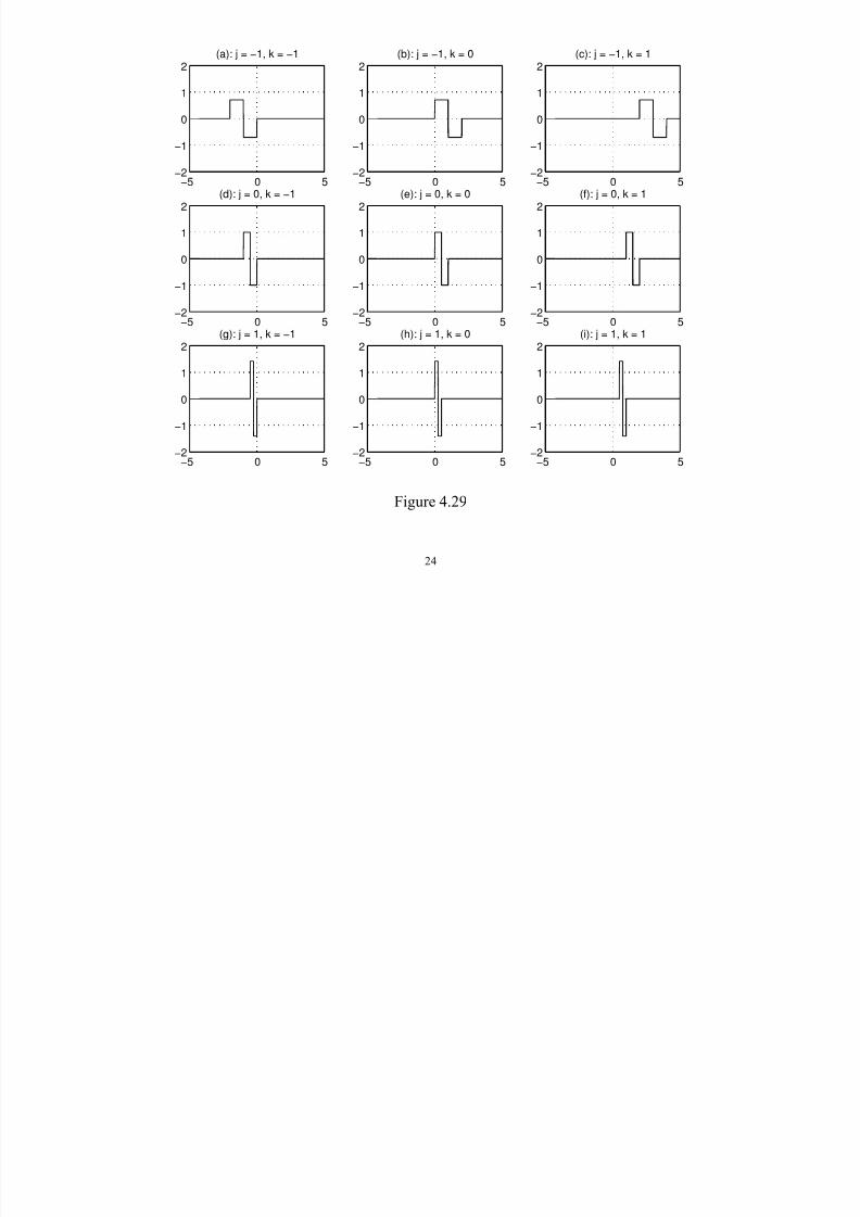
• Dyadic wavelet transform
In the continuous wavelet function
,
1( ) ( )s u
t ut
ssψ ψ
−=
if one chooses 2 and 2 with , integers j js u k j k − −= = ⋅ , then the wavelet
function becomes
/ 2, ( ) 2 (2 ) for , j j
j k t t k j k ψ ψ = − ∈Z (4.55)
Note that here the integer variable j indicates the scale or resolution, with larger j corresponding to higher resolution; and integer variable k represents the
“location” in time axis.

7/29/2019 Notes Wavelets
http://slidepdf.com/reader/full/notes-wavelets 23/74
23
So if the wavelet is quite local, then we can estimate how signal f (t ) is changing
itself in a neighborhood of time instant t * at a given resolution level j by
projecting the signal onto one of the basis functions in (4.55) with 2
j
k t
∗= ⋅.
Example 4.13 With ( )t ψ being the Haar wavelet, Fig. 4.29 shows nine basis
functions , ( ) j k t ψ for j = – 1, 0, 1 and k = – 1, 0, 1. We see that
♦ For each fixed resolution which is determined by the value of index j, the basisfunctions , ( ) j k t ψ have the same width of support and can “move” along the t -axis
to anywhere by using an appropriate value of index k .
♦ The resolution can be increased by using an increased value of index j or decreased by using a decreased value of j.
7/29/2019 Notes Wavelets
http://slidepdf.com/reader/full/notes-wavelets 24/74
24
−5 0 5−2
−1
0
1
2(a): j = −1, k = −1
−5 0 5−2
−1
0
1
2(b): j = −1, k = 0
−5 0 5−2
−1
0
1
2(c): j = −1, k = 1
−5 0 5
−2
−1
0
1
2(d): j = 0, k = −1
−5 0 5
−2
−1
0
1
2(e): j = 0, k = 0
−5 0 5
−2
−1
0
1
2(f): j = 0, k = 1
−5 0 5−2
−1
0
1
2(g): j = 1, k = −1
−5 0 5−2
−1
0
1
2(h): j = 1, k = 0
−5 0 5−2
−1
0
1
2(i): j = 1, k = 1
Figure 4.29
7/29/2019 Notes Wavelets
http://slidepdf.com/reader/full/notes-wavelets 25/74
25
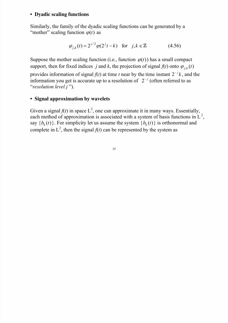
• Dyadic scaling functions
Similarly, the family of the dyadic scaling functions can be generated by a
“mother” scaling function ( )t ϕ as
/ 2, ( ) 2 (2 ) for , j j
j k t t k j k ϕ ϕ = − ∈Z (4.56)
Suppose the mother scaling function (i.e., function ( )t ϕ ) has a small compact
support, then for fixed indices j and k , the projection of signal f (t ) onto , ( ) j k t ϕ
provides information of signal f (t ) at time t near by the time instant 2 jk − , and the
information you get is accurate up to a resolution of 2 j− (often referred to as
“resolution level j ”).
• Signal approximation by wavelets
Given a signal f (t ) in space L2, one can approximate it in many ways. Essentially,
each method of approximation is associated with a system of basis functions in L2,
say { ( )k b t }. For simplicity let us assume the system { ( )k b t } is orthonormal and
complete in L2, then the signal f (t ) can be represented by the system as
7/29/2019 Notes Wavelets
http://slidepdf.com/reader/full/notes-wavelets 26/74
26
( ) ( ), ( ) ( )k k k
f t f t b t b t ∑= (4.57)
A truncation of the first K terms of (4.57) can be used as an approximation of theoriginal signal f (t ), i.e.,
1( ) ( ) ( ), ( ) ( )
K
K k k k
f t f t f t b t b t =
∑≈ = (4.58)
Now suppose we have another orthonormal and complete system of basis
functions { ( )k c t }, hence the signal can also be approximated by a similar
truncation:
1
ˆ( ) ( ) ( ), ( ) ( )K
K k k k
f t f t f t c t c t =
∑≈ = (4.59)
The question is, which approximation, (4.58) or (4.59), is better?
To address this question, we need a quantitative measure for the performance of
an approximation. A general consensus is that an orthonormal and complete
system is considered efficient if a small (relative to other systems) number of
coefficients in the orthogonal expansion are found large in magnitude.
7/29/2019 Notes Wavelets
http://slidepdf.com/reader/full/notes-wavelets 27/74
27
The wavelet theory has shown that basis functions generated from good wavelets
often hold the promise of being efficient systems for signal representation
(compression). As explained below, wavelet and scaling functions come naturally
in signal representations.
Example 4.14 Given a signal f (t ) in L2, first we try to represent it by a staircase
approximation:
( ) ( ) ( )k
f t f k t k ϕ ∞
=−∞≈ −∑ (4.60)
where ( )t ϕ is the Haar scaling function, and f (k ) is the sampled value of f (t ) at t =
k . Fig. 4.30 depicts what happens on interval [–1, 6].
7/29/2019 Notes Wavelets
http://slidepdf.com/reader/full/notes-wavelets 28/74
28
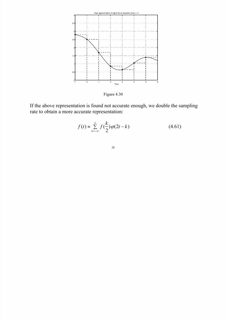
−1 0 1 2 3 4 5 60
0.5
1
1.5
2
2.5
3
3.5
4Haar approximation of signal f(t) at resolution level j = 0
Time
Figure 4.30
If the above representation is found not accurate enough, we double the sampling
rate to obtain a more accurate representation:
( ) ( ) (2 )2k
k f t f t k ϕ
∞
=−∞≈ −∑ (4.61)
7/29/2019 Notes Wavelets
http://slidepdf.com/reader/full/notes-wavelets 29/74
29
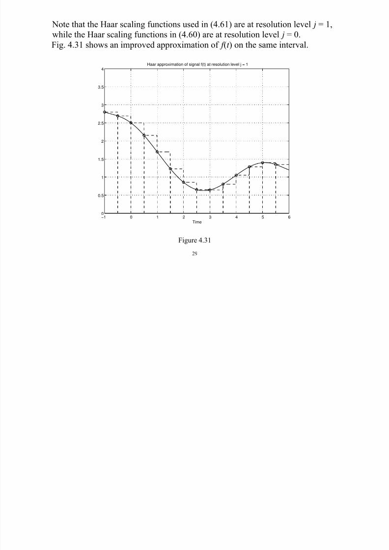
Note that the Haar scaling functions used in (4.61) are at resolution level j = 1,
while the Haar scaling functions in (4.60) are at resolution level j = 0.
Fig. 4.31 shows an improved approximation of f (t ) on the same interval.
−1 0 1 2 3 4 5 60
0.5
1
1.5
2
2.5
3
3.5
4Haar approximation of signal f(t) at resolution level j = 1
Time
Figure 4.31
7/29/2019 Notes Wavelets
http://slidepdf.com/reader/full/notes-wavelets 30/74
30
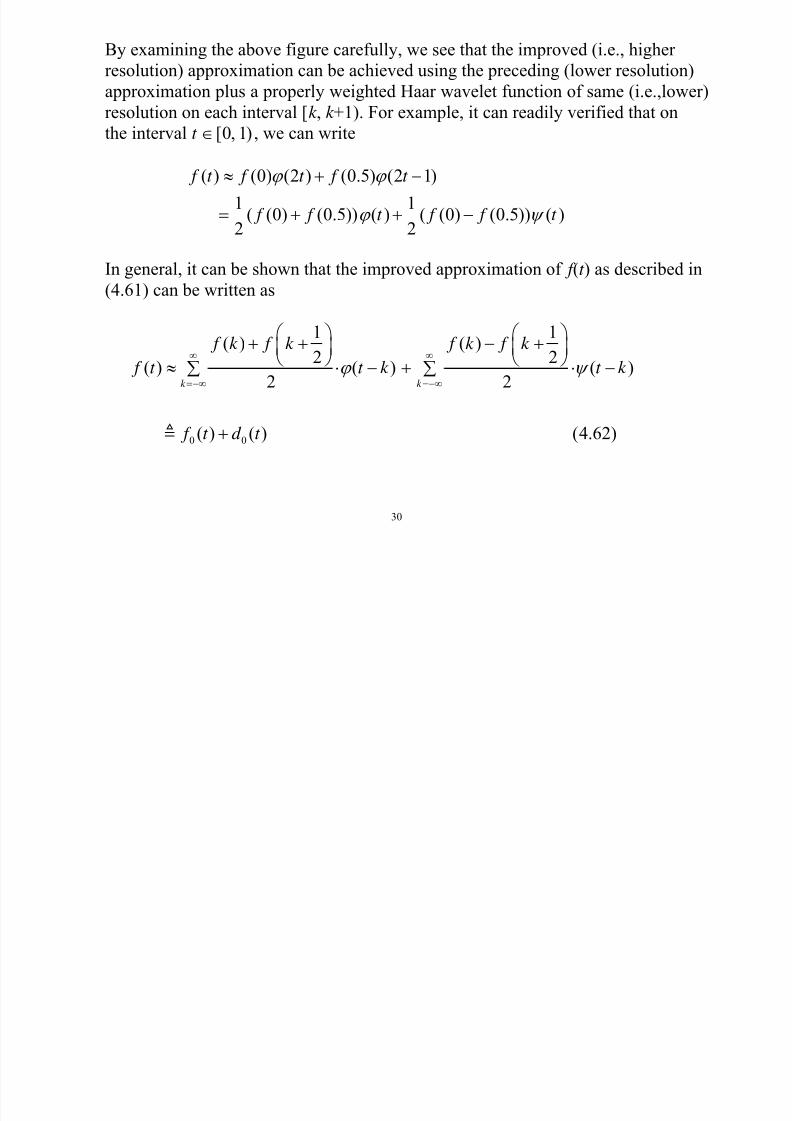
By examining the above figure carefully, we see that the improved (i.e., higher
resolution) approximation can be achieved using the preceding (lower resolution)
approximation plus a properly weighted Haar wavelet function of same (i.e.,lower)
resolution on each interval [k , k +1). For example, it can readily verified that on
the interval t [0, 1)∈ , we can write
( ) (0) (2 ) (0.5) (2 1)
1 1( (0) (0.5)) ( ) ( (0) (0.5)) ( )2 2
f t f t f t
f f t f f t
ϕ ϕ
ϕ ψ
≈ + −
= + + −
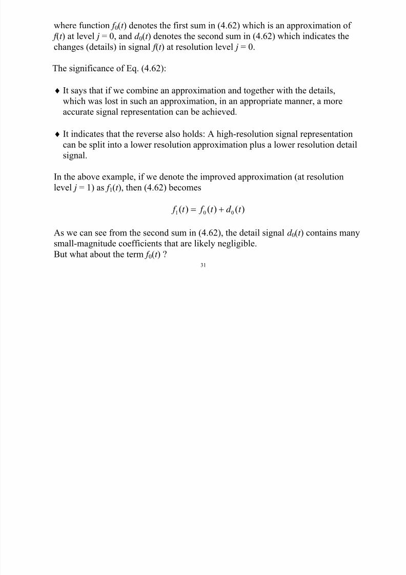
In general, it can be shown that the improved approximation of f (t ) as described in
(4.61) can be written as
0 0
1 1( ) ( )
2 2( ) ( ) ( )
2 2
( ) ( ) (4.62)
k k
f k f k f k f k
f t t k t k
f t d t
ϕ ψ ∞ ∞
=−∞ =−∞
⎛ ⎞ ⎛ ⎞+ + − +⎜ ⎟ ⎜ ⎟
⎝ ⎠ ⎝ ⎠≈ ⋅ − + ⋅ −∑ ∑
+
7/29/2019 Notes Wavelets
http://slidepdf.com/reader/full/notes-wavelets 31/74
31
where function f 0(t ) denotes the first sum in (4.62) which is an approximation of
f (t ) at level j = 0, and d 0(t ) denotes the second sum in (4.62) which indicates the
changes (details) in signal f (t ) at resolution level j = 0.
The significance of Eq. (4.62):
♦ It says that if we combine an approximation and together with the details,
which was lost in such an approximation, in an appropriate manner, a moreaccurate signal representation can be achieved.
♦ It indicates that the reverse also holds: A high-resolution signal representation
can be split into a lower resolution approximation plus a lower resolution detail
signal.
In the above example, if we denote the improved approximation (at resolution
level j = 1) as f 1(t ), then (4.62) becomes
1 0 0( ) ( ) ( ) f t f t d t = +
As we can see from the second sum in (4.62), the detail signal d 0(t ) contains many
small-magnitude coefficients that are likely negligible.
But what about the term f 0(t ) ?

7/29/2019 Notes Wavelets
http://slidepdf.com/reader/full/notes-wavelets 32/74
32
We can apply the same idea of “splitting a signal into lower resolution
approximation and detail components” to f 0(t ) to obtain
0 1 1( ) ( ) ( ) f t f t d t − −= +
where d -1(t ) denotes the details at resolution level j = – 1 , which likely contains
many small-coefficient terms, and f -1(t ) denote the signal’s approximation atresolution j = – 1.
It is important to stress that in practice signals in many DSP applications are of
finite length, often representing the sampled values of continuous-time signals in
certain finite time duration. In such cases, as the decomposition proceeds the totalnumber of terms in lower resolution approximation components decrease at rate
12− .
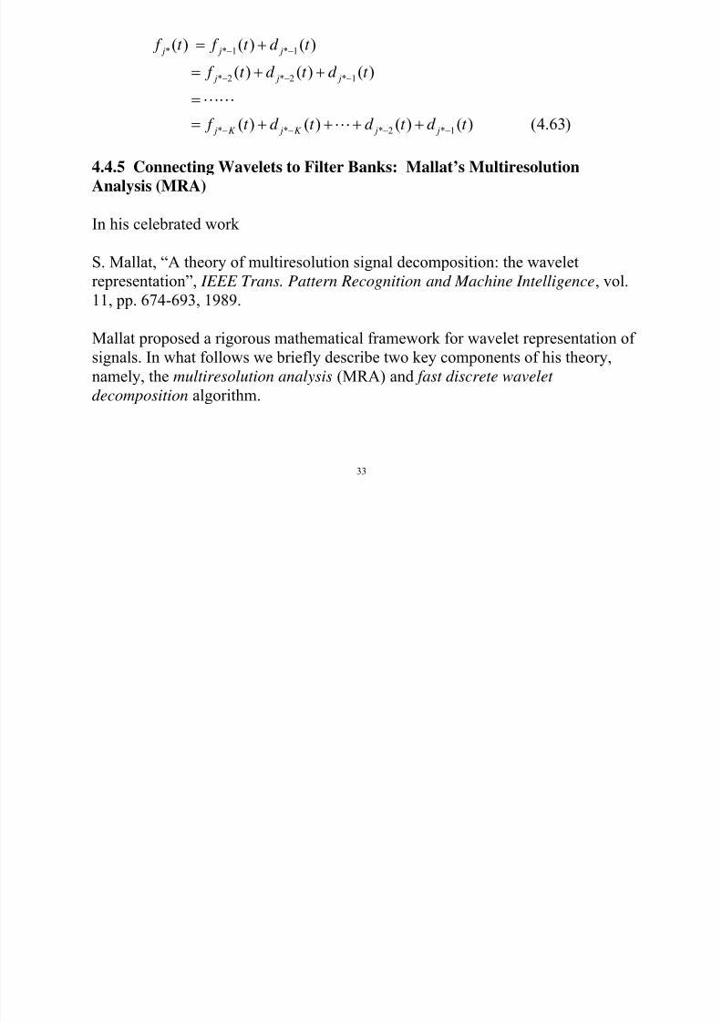
In general, let the signal of interest be given at a certain resolution level, say, j =
j*, as f j*(t ). Then an efficient representation of f (t ) can be obtained as
( ) ( ) ( )f f d
7/29/2019 Notes Wavelets
http://slidepdf.com/reader/full/notes-wavelets 33/74
33
* * 1 * 1
* 2 * 2 * 1
* * * 2 * 1
( ) ( ) ( )
( ) ( ) ( )
( ) ( ) ( ) ( ) (4.63)
j j j
j j j
j K j K j j
f t f t d t
f t d t d t
f t d t d t d t
− −
− − −
− − − −
= +
= + +
== + + + +
4.4.5 Connecting Wavelets to Filter Banks: Mallat’s Multiresolution
Analysis (MRA)
In his celebrated work
S. Mallat, “A theory of multiresolution signal decomposition: the wavelet
representation”, IEEE Trans. Pattern Recognition and Machine Intelligence, vol.
11, pp. 674-693, 1989.
Mallat proposed a rigorous mathematical framework for wavelet representation of
signals. In what follows we briefly describe two key components of his theory,namely, the multiresolution analysis (MRA) and fast discrete wavelet
decomposition algorithm.
M ll ’ M l i l i A l i
7/29/2019 Notes Wavelets
http://slidepdf.com/reader/full/notes-wavelets 34/74
34
• Mallat’s Multiresolution Analysis
A sequence { , } j
V j ∈Z of closed subspaces of L2 is said to be a multiresolution
approximation if the following properties hold:
(1) For every 2( , ) , ( ) ( 2 ) j
j j j k f t V f t k V
−∈ ∈ ⇔ − ∈Z
(2) 1For every , j j j V V +∈ ⊂Z
(3) 1For every , ( ) (2 ) j j
j f t V f t V +∈ ∈ ⇔ ∈Z
(4) 2Llim j j
V →∞
=
(5) {0}lim j j
V →−∞
=
(6) There exists ( ) such that { ( ), }t t k k ϕ ϕ − ∈Z is a Riesz basis of subspace V 0.
The rationale of the MRA can be easily understood by using the Haar scaling
function as ( )t ϕ in property (6). One can think of subspace V j as a place that
collects all the signals with resolution level j. If we have to deal with a signal withresolution higher than j, then by property (4) we know that it is contained in some
subspace V k with k > j.
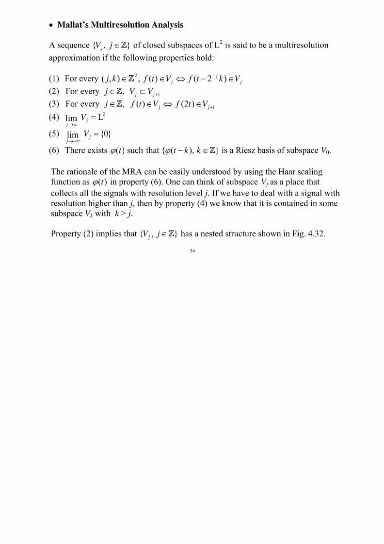
Property (2) implies that { , } jV j ∈Z has a nested structure shown in Fig. 4.32.
7/29/2019 Notes Wavelets
http://slidepdf.com/reader/full/notes-wavelets 35/74
35
V 1
V 0
V -1
Figure 4.32
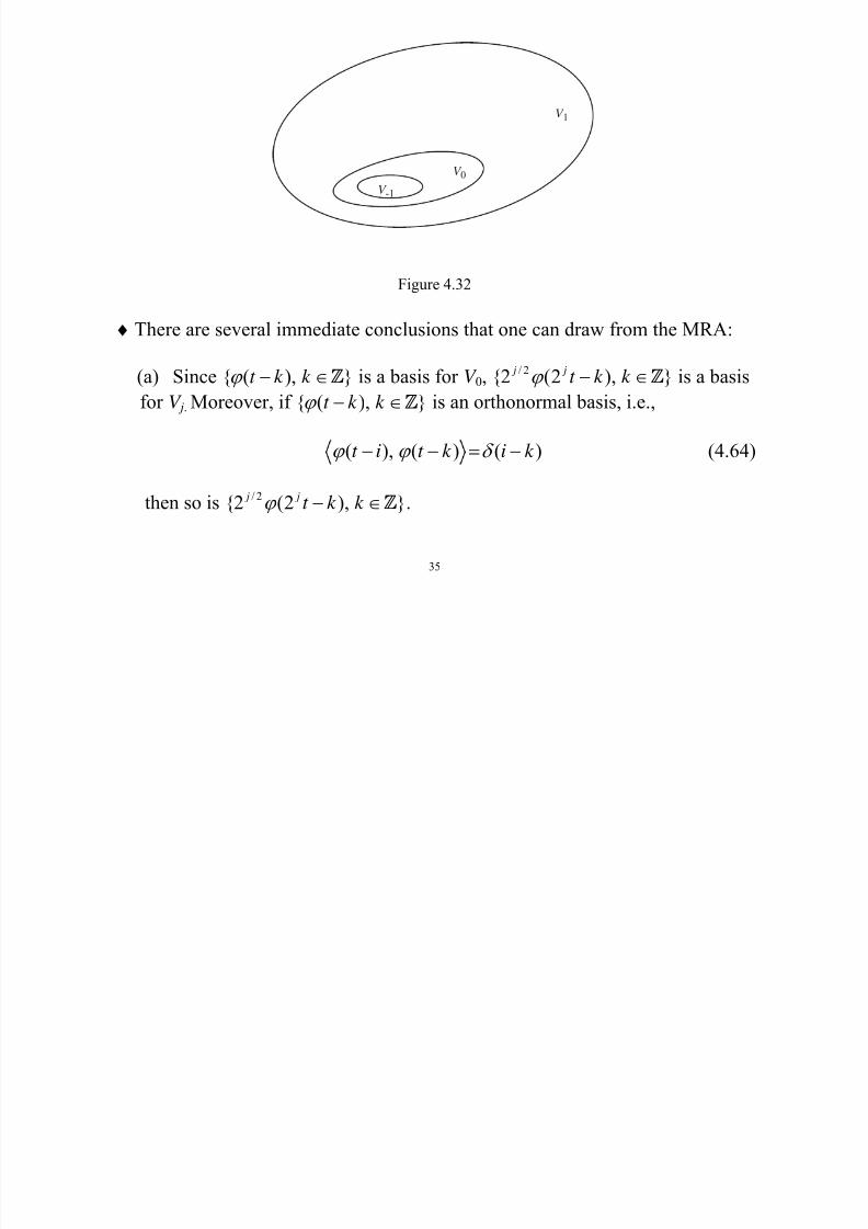
♦ There are several immediate conclusions that one can draw from the MRA:
(a) Since { ( ), }t k k ϕ − ∈Z is a basis for V 0,/ 2{2 (2 ), } j j
t k k ϕ − ∈Z is a basis
for V j. Moreover, if { ( ), }t k k ϕ − ∈Z is an orthonormal basis, i.e.,
( ), ( ) ( )t i t k i k ϕ ϕ δ − − = − (4.64)
then so is/ 2
{2 (2 ), } j j t k k ϕ − ∈Z .
7/29/2019 Notes Wavelets
http://slidepdf.com/reader/full/notes-wavelets 36/74
36
(b) Since0 1( )t V V ϕ ∈ ⊂ , ( )t ϕ cab be expressed in V 1 as
( ) 2 (2 )k k
t h t k ϕ ϕ ∞
=−∞= −∑ (4.65)
Eq. (4.65) is called the dilation equation, which is one of the key equations in
wavelet theory.
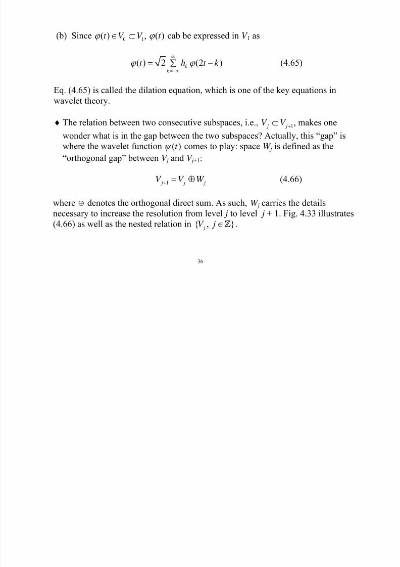
♦ The relation between two consecutive subspaces, i.e., 1 j jV V +⊂ , makes one
wonder what is in the gap between the two subspaces? Actually, this “gap” is
where the wavelet function ( )t ψ comes to play: space W j is defined as the
“orthogonal gap” between V j and V j+1:
1 j j jV V W + = ⊕ (4.66)
where ⊕ denotes the orthogonal direct sum. As such, W j carries the detailsnecessary to increase the resolution from level j to level j + 1. Fig. 4.33 illustrates
(4.66) as well as the nested relation in { , } jV j ∈Z .

7/29/2019 Notes Wavelets
http://slidepdf.com/reader/full/notes-wavelets 37/74
37
V 1
V 0
W 0
Figure 4.33
♦ Based on (4.66) and MRA properties (4) and (5), we can write
1
1 1
2 (4.67)
j j j
j j j
jk k
j j
V V W
V W W
W
L W
+
− −
=−∞
∞=−∞
= ⊕
= ⊕ ⊕
=
= ⊕⇒ = ⊕
Eq. (4.67) gives an orthogonal decomposition of space L2. It implies that for a
finite-energy signal f (t ) in L2, we have
7/29/2019 Notes Wavelets
http://slidepdf.com/reader/full/notes-wavelets 38/74
38
( ) ( )W j j
f t P f t ∞
=−∞∑= (4.68)
where Pwj denote the orthogonal projection operator onto space W j. Since spaces
W j collect details of the signal, many terms in (4.68) are likely small and can
therefore be neglected to obtain an accurate yet efficient representation of f (t ).
Now suppose that subspace W 0 admits a basis { ( ),t k k ψ − ∈Z} which is
generated by a wavelet function ( )t ψ , then we (4.66) implies that
0 1( )t W V ψ ∈ ⊂
which means that ( )t ψ can be expressed as an element in V 1 as
( ) (2 )k
k
t g t k ψ ϕ ∞
=−∞
∑= − (4.69)
This important equation is called the wavelet equation. It follows that once thescaling function ( )t ϕ has been determined, (4.69) can be used to compute the
wavelet function ( )t ψ , provided that the coefficients { , }k g k ∈Z are available.
• Orthogonal Wavelets and Orthogonal Filter Banks
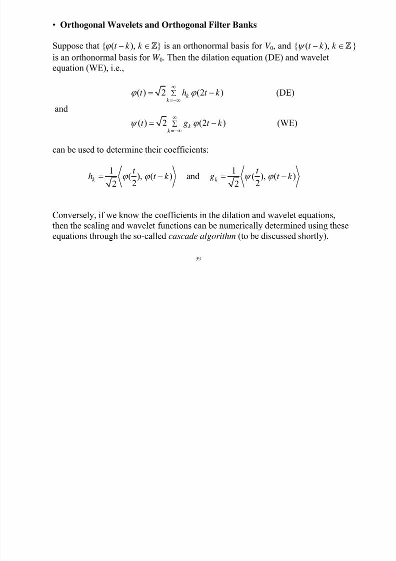
7/29/2019 Notes Wavelets
http://slidepdf.com/reader/full/notes-wavelets 39/74
39
Orthogonal Wavelets and Orthogonal Filter Banks
Suppose that { ( ), }t k k ϕ − ∈Z is an orthonormal basis for V 0, and { ( ),t k k ψ − ∈Z}
is an orthonormal basis for W 0. Then the dilation equation (DE) and wavelet
equation (WE), i.e.,
( ) 2 (2 )k
k
t h t k ϕ ϕ ∞
=−∞
∑= − (DE)
and
( ) 2 (2 )k k
t g t k ψ ϕ ∞
=−∞∑= − (WE)
can be used to determine their coefficients:
1( ), ( )22
k
t h t k ϕ ϕ = − and
1( ), ( )22
k
t g t k ψ ϕ = −
Conversely, if we know the coefficients in the dilation and wavelet equations,
then the scaling and wavelet functions can be numerically determined using these
equations through the so-called cascade algorithm (to be discussed shortly).
The number of terms in the DE and WE will be reduced to N for compactly
7/29/2019 Notes Wavelets
http://slidepdf.com/reader/full/notes-wavelets 40/74
40
The number of terms in the DE and WE will be reduced to N for compactly
supported wavelet functions such as Haar and Daubechies orthogonal wavelets,
where N is the length of the associated filters H 0( z), etc.
For example, it is easy to examine that for the Haar scaling and wavelet functions,
the DE and WE simply become
1 1( ) 2 (2 ) (2 1)2 2
t t t ϕ ϕ ϕ ⎡ ⎤= + −⎢ ⎥⎣ ⎦(4.70)
and1 1
( ) 2 (2 ) (2 1)2 2
t t t ψ ϕ ϕ ⎡ ⎤
= − −⎢ ⎥⎣ ⎦(4.71)
We see that the coefficients in (4.70) and (4.71) are the impulse responses of the
lowpass and highpass synthesis filters in the orthogonal Haar filter bank,
respectively. This connection holds for any compactly supported orthogonal
scaling and wavelet functions.
In particular, the Daubechies scaling function is defined by
1 N −
∑

7/29/2019 Notes Wavelets
http://slidepdf.com/reader/full/notes-wavelets 41/74
41
0
( ) 2 (2 )k
k
t h t k ϕ ϕ =
= −∑ (4.72)
where {hk , k = 0, …, N – 1} are the coefficients of the lowpass synthesis filter
F 0( z).
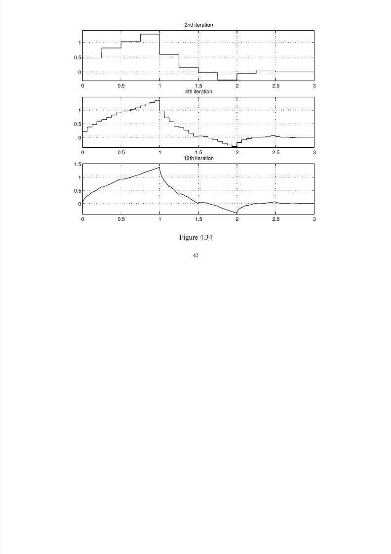
The following iterative algorithm, known as the cascade
algorithm, can be used to determine the numerical values of the scaling function( )t ϕ on its support interval [0, N – 1]:
1( 1) ( )
0( ) 2 (2 )
N i i
k k
t h t k ϕ ϕ −+
=∑= − (4.73)
for i = 0, 1, …, with(0)
( )t ϕ being the Haar scaling function. Convergence of the
algorithm is deemed when
( 1) ( )
2( ) ( )i i
t t ϕ ϕ ε +
− ≤
for a prescribed tolerance ε . Fig. 4.34 shows the 2nd, 4th and 12th iteration results
of the cascade algorithm as applied to the Daubechies filter of length 4 (D4).
2nd iteration
7/29/2019 Notes Wavelets
http://slidepdf.com/reader/full/notes-wavelets 42/74
42
0 0.5 1 1.5 2 2.5 3
0
0.5
1
0 0.5 1 1.5 2 2.5 3
0
0.5
1
4th iteration
0 0.5 1 1.5 2 2.5 3
0
0.5
1
1.512th iteration
Figure 4.34
=== MATLAB code of the cascade algorithm ===
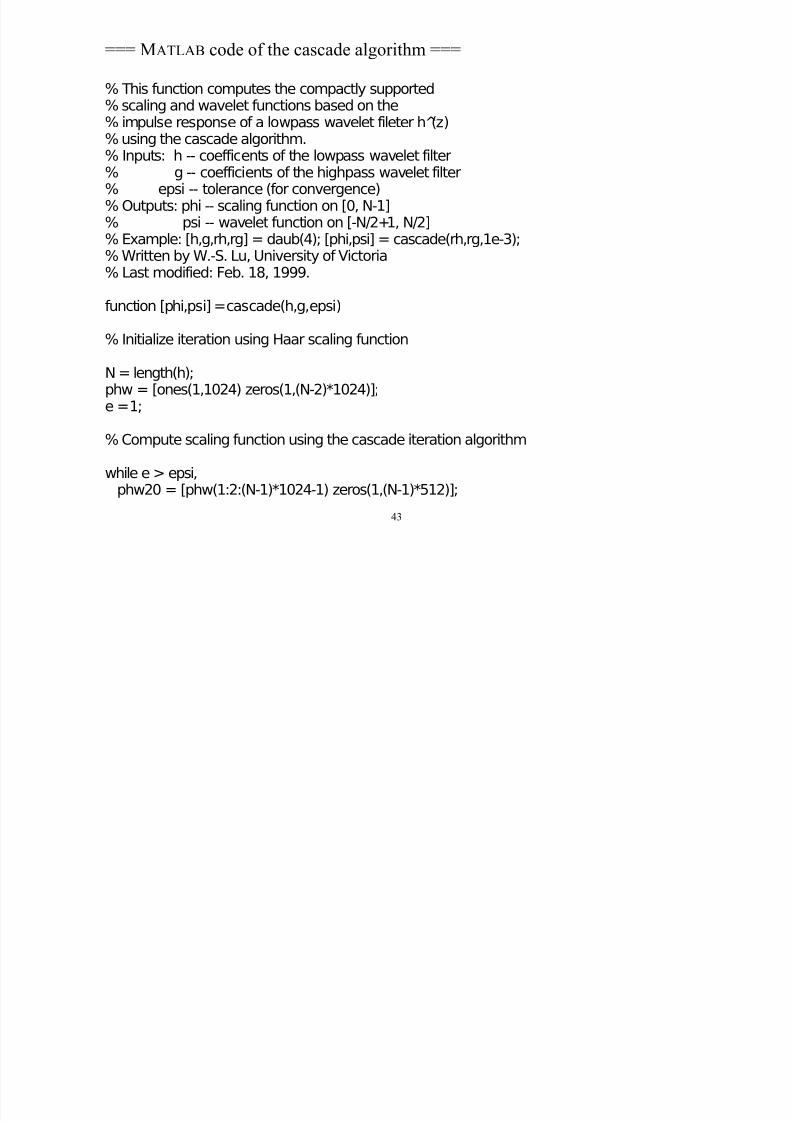
7/29/2019 Notes Wavelets
http://slidepdf.com/reader/full/notes-wavelets 43/74
43
g
% This function computes the compactly supported
% scaling and wavelet functions based on the% impulse response of a lowpass wavelet fileter h (̂z)% using the cascade algorithm.% Inputs: h -- coefficents of the lowpass wavelet filter% g -- coefficients of the highpass wavelet filter% epsi -- tolerance (for convergence)
% Outputs: phi -- scaling function on [0, N-1]% psi -- wavelet function on [-N/2+1, N/2]% Example: [h,g,rh,rg] = daub(4); [phi,psi] = cascade(rh,rg,1e-3);% Written by W.-S. Lu, University of Victoria% Last modified: Feb. 18, 1999.
function [phi,psi] = cascade(h,g,epsi)
% Initialize iteration using Haar scaling function
N = length(h);phw = [ones(1,1024) zeros(1,(N-2)*1024)];e = 1;
% Compute scaling function using the cascade iteration algorithm
while e > epsi,
phw20 = [phw(1:2:(N-1)*1024-1) zeros(1,(N-1)*512)];
phw2 = h(1)*phw20;f k 1 N 1
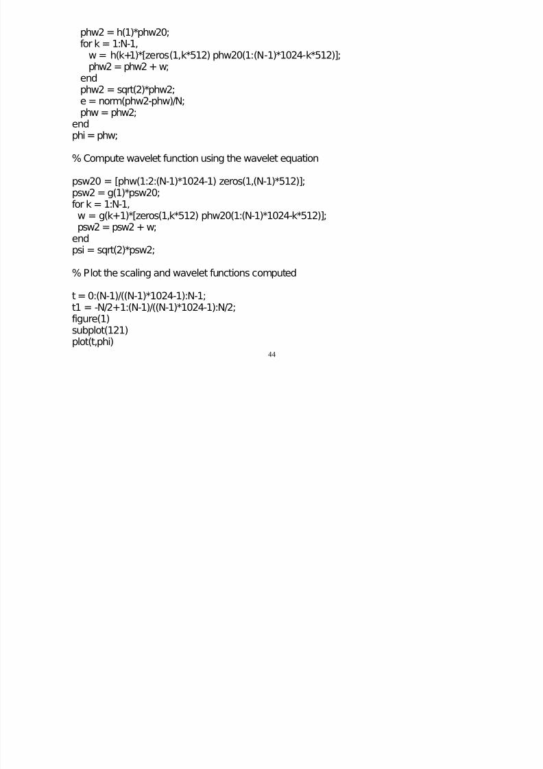
7/29/2019 Notes Wavelets
http://slidepdf.com/reader/full/notes-wavelets 44/74
44
for k = 1:N-1,w = h(k+1)*[zeros(1,k*512) phw20(1:(N-1)*1024-k*512)];phw2 = phw2 + w;
endphw2 = sqrt(2)*phw2;e = norm(phw2-phw)/N;phw = phw2;
end
phi = phw;
% Compute wavelet function using the wavelet equation
psw20 = [phw(1:2:(N-1)*1024-1) zeros(1,(N-1)*512)];psw2 = g(1)*psw20;
for k = 1:N-1,w = g(k+1)*[zeros(1,k*512) phw20(1:(N-1)*1024-k*512)];psw2 = psw2 + w;
endpsi = sqrt(2)*psw2;
% Plot the scaling and wavelet functions computed
t = 0:(N-1)/((N-1)*1024-1):N-1;t1 = -N/2+1:(N-1)/((N-1)*1024-1):N/2;figure(1)subplot(121)
plot(t,phi)
axis([0 N-1 1.1*min(phi) 1.1*max(phi)])i (' ')
7/29/2019 Notes Wavelets
http://slidepdf.com/reader/full/notes-wavelets 45/74
45
axis('square')gridtitle('scaling function')xlabel('time')subplot(122)plot(t1,psi)axis([-N/2+1 N/2 1.1*min(psi) 1.1*max(psi)])axis('square')
gridtitle('wavelet function')xlabel('time')
Once ( )t ϕ is found, the wavelet function can be obtained using the wavelet
equation1
( 2)
( ) 2 (2 )k
k N
t g t k ψ ϕ =− −
= −∑ (4.74)
where {gk , k = - ( N – 2) , …, 0, 1} are the coefficients of the highpass synthesisfilter F 1( z) with their indices shifted backwards by – ( N – 2).
Note that ( )t ψ has a support on [1- N /2, N /2].
The orthogonal Daubechies wavelets of length N has p = N /2 vanishing moments.
Fig. 4.35 shows the Daubechies scaling and wavelet functions with p = 2, 3, and 4
vanishing moments.
7/29/2019 Notes Wavelets
http://slidepdf.com/reader/full/notes-wavelets 46/74
46
• Mallat’s Fast Wavelet Transform (FWT)
Let a finite-energy signal f (t ) be in space V j+1 so that it can be expressed as
( 1) / 2 ( 1) 1( ) 2 (2 ) j j j
k
k
f t a t k ϕ ∞
+ + +
=−∞
= −∑ (4.75)
Since 1 j j jV V W + = ⊕ , f (t ) can be decomposed as
/ 2 ( )
/ 2 ( )
( ) ( ) ( )
where
2 (2 )
2 (2 )
j j
j
j
V W
j j j
V k
k
j j j
W k k
f t P f t P f t
P f a t k
P f d t k
ϕ
ψ
= +
= −
= −
∑
∑
with ( ) and ( )t t ϕ ψ being a pair of orthogonal scaling and wavelet functions.
1 5scaling function N = 4, p = 2 wavelet function N = 4, p = 2
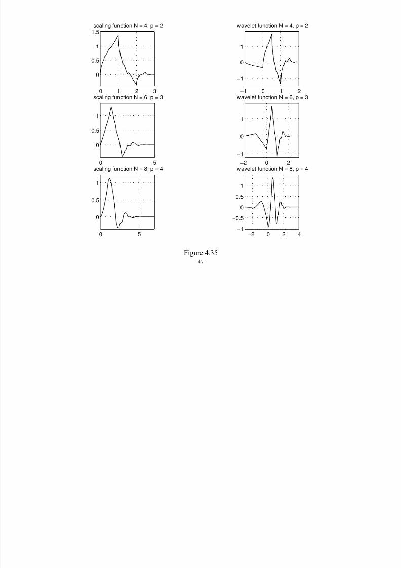
7/29/2019 Notes Wavelets
http://slidepdf.com/reader/full/notes-wavelets 47/74
47
0 1 2 3
0
0.5
1
1.5
−1 0 1 2
−1
0
1
0 5
0
0.5
1
scaling function N = 6, p = 3
−2 0 2−1
0
1
wavelet function N = 6, p = 3
0 5
0
0.5
1
scaling function N = 8, p = 4
−2 0 2 4−1
−0.5
0
0.5
1
wavelet function N = 8, p = 4
Figure 4.35
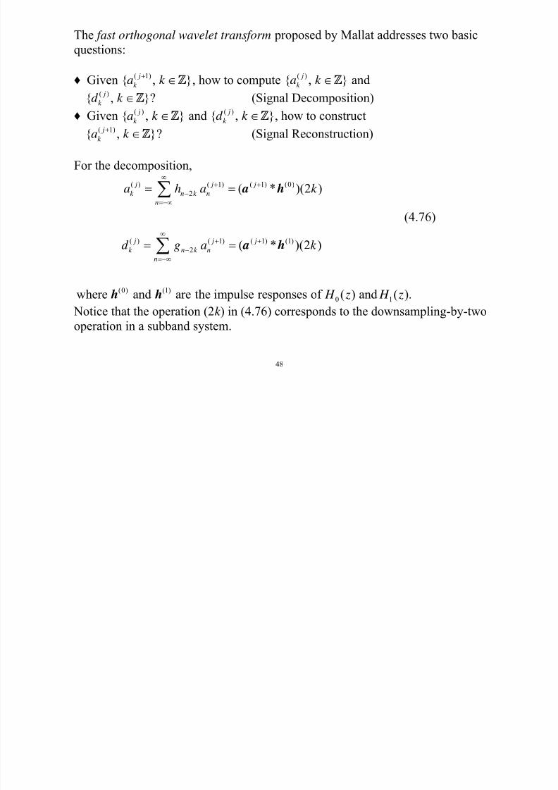
The fast orthogonal wavelet transform proposed by Mallat addresses two basic
i
7/29/2019 Notes Wavelets
http://slidepdf.com/reader/full/notes-wavelets 48/74
48
questions:
♦ Given ( 1){ , } jk a k + ∈Z , how to compute ( ){ , } j
k a k ∈Z and( ){ , } j
k d k ∈Z ? (Signal Decomposition)
♦ Given( ){ , } j
k a k ∈Z and
( ){ , } j
k d k ∈Z , how to construct
( 1){ , } j
k a k
+ ∈Z ? (Signal Reconstruction)
For the decomposition,
( ) ( 1) ( 1) (0)
2
( ) ( 1) ( 1) (1)
2
(0) (1)
0 1
( * )(2 )
(4.76)
( * )(2 )
where and are the impulse responses of ( ) and ( ).
j j j
k n k n
n
j j j
k n k n
n
a h a k
d g a k
H z H z
∞+ +
−=−∞
∞+ +
−=−∞
= =
= =
∑
∑
a h
a h
h h
Notice that the operation (2k ) in (4.76) corresponds to the downsampling-by-two
operation in a subband system.
For the reconstruction,

7/29/2019 Notes Wavelets
http://slidepdf.com/reader/full/notes-wavelets 49/74
49
( 1) ( ) ( )
2 2
( ) ( )
( ) ( )
( ) ( )
( * )( ) ( * )( ) (4.77)
where
if 2 if 2and0 if 2 1 0 if 2 1
j j j
k k n n k n nk k
j j
j j
j j p p
k k
a h a g d
k k
a k p d k pa d k p k p
∞ ∞+
− −=−∞ =−∞= +
= +
⎧ ⎧= == =⎨ ⎨= + = +⎩ ⎩
∑ ∑
a h d g
Notice that the operation required to generate signals ( ) ( )and j j
a d from( ) ( )
and j j
a d in (4.77) corresponds to the upsampling-by-two operation in asubband system. Therefore, together (4.76) and (4.77) admit a 2-channel filter-
bank interpretation with a( j+1) as its input signal.
Based on (4.76) and (4.77), a K -level fast signal decomposition and reconstruction
can be carried out in an MRA framework as follows, where signal f (t ) correspondsto a( J ) :
It is quite obvious that the above decomposition and reconstruction can be
implemented using an orthogonal filter bank with a K -level tree structure, where
the coefficients of the synthesis lowpass and highpass filters are obtained from
DE d WE ti l
7/29/2019 Notes Wavelets
http://slidepdf.com/reader/full/notes-wavelets 50/74
50
DE and WE, respectively.
References1. I. Daubechies, “Orthogonal bases of compactly supported wavelets,” Comm. on Pure and Appl.
Math., vol. 41, pp. 909-996, Nov. 1988.
2. I. Daubechies, Ten Lectures on Wavelets, SIAM, Philadelphia, PA, 1992.
3. S. Mallat, “A theory for multiresolution signal decomposition: the wavelet representation,” IEEE
Trans. PRMI , vol. 11, pp. 674-693, July, 1989.
4. S. Mallat, A Wavelet Tour of Signal Processing, 2nd ed., Academic Press, New York, 1999.
7.1 Wavelet De-Noising
7.1.1 The de-noising problem
Suppose we have a noise-corrupted discrete-time signal x[n], which is modeled as
noisy signal noisesignal
[ ] [ ] [ ] 0,1,..., 1 x n s n w n n N = + = − (7.1)
where s[n] is the noise-free signal, and w[n] is noise with n = 0, 1, …, N – 1.
The de-noising problem is to estimate s[n] using the noise-corrupted observations
x[n]. In what follows we present a de-noising method based on discrete wavelet
transform (or equivalently subband decomposition) of the noisy signal x[n] The
7/29/2019 Notes Wavelets
http://slidepdf.com/reader/full/notes-wavelets 51/74
51
transform (or equivalently subband decomposition) of the noisy signal x[n]. The
method was proposed by David Donoho and Ian Johnstone in 1993.
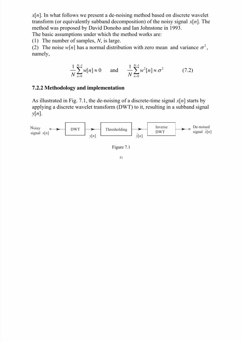
The basic assumptions under which the method works are:(1) The number of samples, N , is large.
(2) The noise w[n] has a normal distribution with zero mean and variance2
σ ,
namely,
1 12 2
0 0
1 1[ ] 0 and [ ]
N N
n n
w n w n N N
σ − −
= =
≈ ≈∑ ∑ (7.2)
7.2.2 Methodology and implementation
As illustrated in Fig. 7.1, the de-noising of a discrete-time signal x[n] starts by
applying a discrete wavelet transform (DWT) to it, resulting in a subband signal
y[n].
oisy
signal x[n] y[n] y[n]^
De-noised
signal x[n]^DWT ThresholdingInverse
DWT
Figure 7.1
From Chapter 4 we know that the DWT of x[n] can be performed by repeatedly
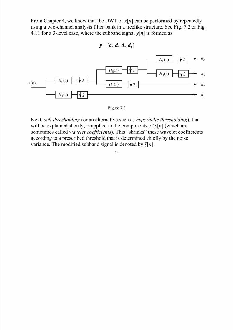
7/29/2019 Notes Wavelets
http://slidepdf.com/reader/full/notes-wavelets 52/74
52
From Chapter 4, we know that the DWT of x[n] can be performed by repeatedly
using a two-channel analysis filter bank in a treelike structure. See Fig. 7.2 or Fig.
4.11 for a 3-level case, where the subband signal y[n] is formed as
3 3 2 1[ ]= y a d d d
H 0( z)
d 1
d 2
d 3
a3
H 1( z)
2
2
H 0( z)
H 1( z)
2
2
H 0( z)
H 1( z)
2
2
(n)
Figure 7.2
Next, soft thresholding (or an alternative such as hyperbolic thresholding), thatwill be explained shortly, is applied to the components of y[n] (which are
sometimes called wavelet coefficients). This “shrinks” these wavelet coefficients
according to a prescribed threshold that is determined chiefly by the noise
variance. The modified subband signal is denoted by ˆ[ ] y n .
Finally, the inverse DWT is applied the modified subband signal ˆ[ ] y n to construct
a discrete time signal ˆ[ ]x n which hopefully would offer a less noisy profile of the

7/29/2019 Notes Wavelets
http://slidepdf.com/reader/full/notes-wavelets 53/74
53
a discrete-time signal [ ] x n which hopefully would offer a less noisy profile of the
original (clear) signal s[n]. It follows from Chapter 4 that the inverse DWT can be
implemented using a tree type filter-bank structure which is mirror-image
symmetrical to that in Fig. 7.2, where the analysis filters H0 and H1 are replaced
with synthesis filters F0 and F1, respectively, and the downsamplers are replaced
by upsamplers. See Fig. 7.3 for a 3-level inverse DWT.
F 0( z)
d 1
d 2
d 3
a3
F 1( z)
2
F 0( z)
F 1( z)
F 0( z)
F 1( z)
2
22
2
2
x (n)^
Figure 7.3
• Thresholding (shrinkage) policies
There are several ways in which thresholding of a given signal may be performed
for a given threshold δ :
(1) Hard thresholding
7/29/2019 Notes Wavelets
http://slidepdf.com/reader/full/notes-wavelets 54/74
54
hard
[ ] if [ ]
[ ] 0 if [ ]
y n y n
y n y n
δ
δ
>⎧
= ⎨ ≤⎩ (7.3a)
(2) Soft thresholding
sof
sgn( [ ])( [ ] ) if [ ][ ]
0 if [ ]t
y n y n y n y n
y n
δ δ
δ − >⎧= ⎨
≤⎩(7.3b)
(3) Hyperbolic thresholding (proposed by B. Vidakovic, also known as “almost
hard thresholding”)
2 2
hyper
sgn( [ ]) [ ] if [ ][ ]
0 if [ ]
y n y n y n y n
y n
δ δ
δ
⎧ − >⎪= ⎨
≤⎪⎩(7.3c)
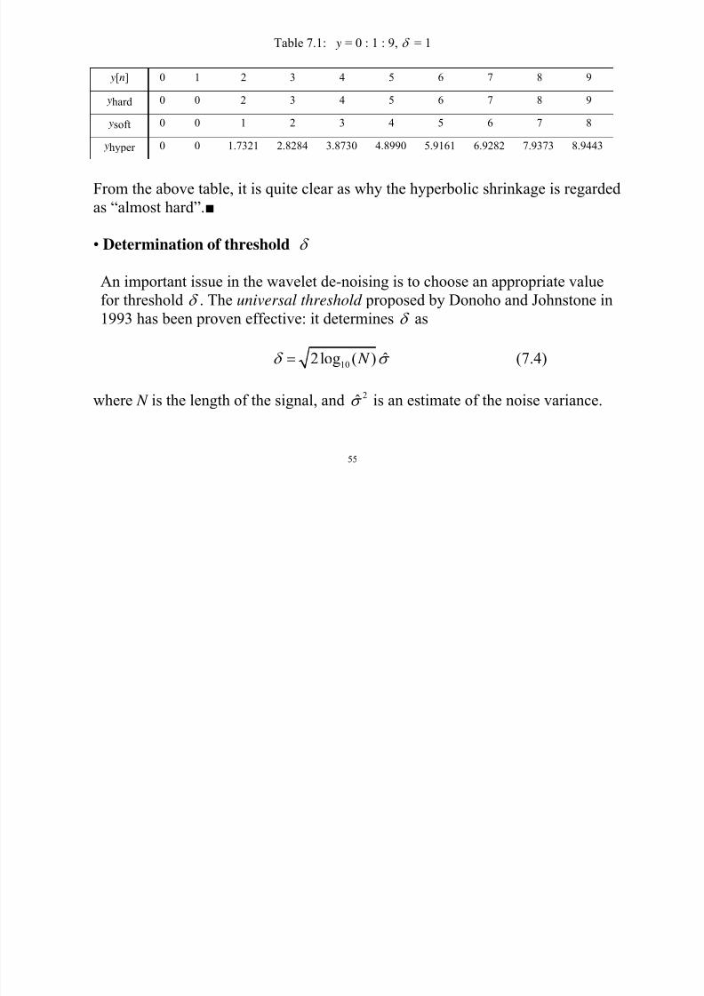
Example 7.1 For y[n] = 0:1:9 and δ = 1, evaluate yhard, ysoft, and yhyper .
The evaluation results are given in Table 7.1.
Table 7.1: y = 0 : 1 : 9, δ = 1
7/29/2019 Notes Wavelets
http://slidepdf.com/reader/full/notes-wavelets 55/74
55
y[n] 0 1 2 3 4 5 6 7 8 9
yhard 0 0 2 3 4 5 6 7 8 9
ysoft 0 0 1 2 3 4 5 6 7 8
yhyper 0 0 1.7321 2.8284 3.8730 4.8990 5.9161 6.9282 7.9373 8.9443
From the above table, it is quite clear as why the hyperbolic shrinkage is regardedas “almost hard”.■
• Determination of threshold δ
An important issue in the wavelet de-noising is to choose an appropriate value
for threshold δ . The universal threshold proposed by Donoho and Johnstone in
1993 has been proven effective: it determines δ as
102log ( ) ˆ N δ σ = (7.4)
where N is the length of the signal, and 2σ̂ is an estimate of the noise variance.
A convenient way to estimate noise variance 2σ is to use the detail subsignal at
the highest resolution i e d1 Let d1 = { (1)d i = 1 N/2} then an estimate of
7/29/2019 Notes Wavelets
http://slidepdf.com/reader/full/notes-wavelets 56/74
56
the highest resolution, i.e., d 1. Let d 1 {i
d , i 1, …, N /2}, then an estimate of 2σ can be obtained as
/ 2 / 22 (1) 2 (1)
1
1 1
2 2( ) where mean( )ˆ
( 2)
N N
i i
i i
d d d d N N
σ = =
= − = =−
∑ ∑ d (7.5)
Example 7.2 We now apply the above de-noising method with various waveletsand shrinkage policies to several noise-corrupted signals.
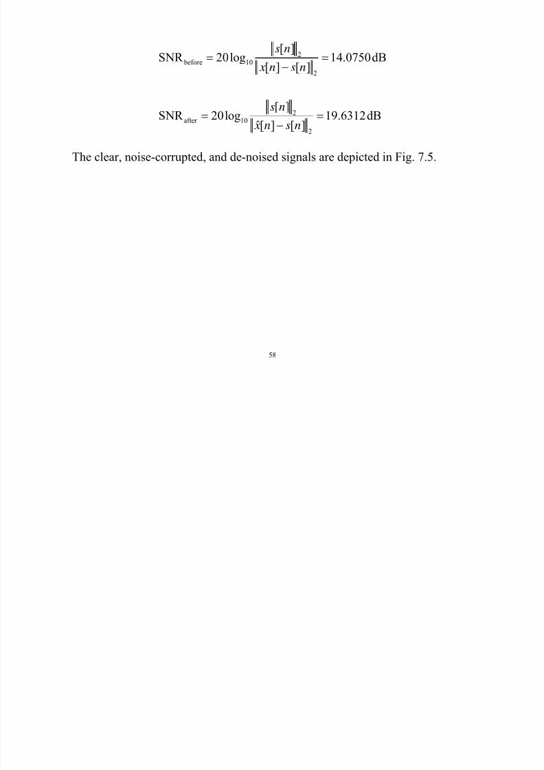
1. Piecewise constant signal (1024 samples, see Fig. 7.4).
Noise: 2(0, )σ N that is a random noise sequence of normal distribution with zero
mean and variance
2σ , where
2σ = 0.0107.
Wavelet: Haar
Shrinkage: Hyperbolic
Threshold: Universal
Results: The signal-to-noise ratio (SNR) before and after de-noising are denoted by SNR before and SNR after , respectively, where
2 before 10
[ ]SNR 20log 27.1056dB
[ ] [ ]
s n
x n s n= =
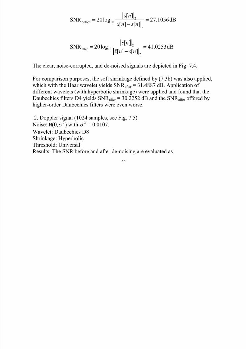
7/29/2019 Notes Wavelets
http://slidepdf.com/reader/full/notes-wavelets 57/74
57
2
2after 10
2
[ ] [ ]
[ ]SNR 20log 41.0253dB
[ ] [ ]ˆ
x n s n
s n
x n s n
−
= =−
The clear, noise-corrupted, and de-noised signals are depicted in Fig. 7.4.
For comparison purposes, the soft shrinkage defined by (7.3b) was also applied,
which with the Haar wavelet yields SNR after = 31.4887 dB. Application of
different wavelets (with hyperbolic shrinkage) were applied and found that the
Daubechies filters D4 yields SNR after = 30.2252 dB and the SNR after offered by
higher-order Daubechies filters were even worse.
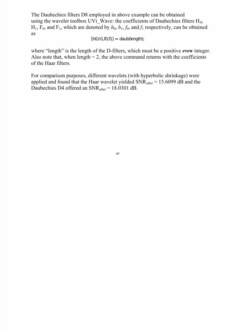
2. Doppler signal (1024 samples, see Fig. 7.5)
Noise:2
(0, )σ N with2
σ
= 0.0107.Wavelet: Daubechies D8
Shrinkage: Hyperbolic
Threshold: Universal
Results: The SNR before and after de-noising are evaluated as
2[ ]
SNR 20l 14 0750dBs n
7/29/2019 Notes Wavelets
http://slidepdf.com/reader/full/notes-wavelets 58/74
58
2 before 10
2
2after 10
2
[ ]SNR 20log 14.0750dB
[ ] [ ]
[ ]SNR 20log 19.6312dB
[ ] [ ]ˆ
x n s n
s n
x n s n
= =−
= =−
The clear, noise-corrupted, and de-noised signals are depicted in Fig. 7.5.
5
original signal0.4
the noise
7/29/2019 Notes Wavelets
http://slidepdf.com/reader/full/notes-wavelets 59/74
59
0 0.5 1
−2
−1
0
1
2
3
4
5
0 0.5 1−0.3
−0.2
−0.1
0
0.1
0.2
0.3
0 0.5 1
−2
−1
0
1
2
3
4
5
noise−contaminated signal
0 0.5 1
−2
−1
0
1
2
3
4
5
denoised signal
Figure 7.4
The Daubechies filters D8 employed in above example can be obtained
using the wavelet toolbox UVi_Wave: the coefficients of Daubechies filters H0,
7/29/2019 Notes Wavelets
http://slidepdf.com/reader/full/notes-wavelets 60/74
60
H1, F0, and F1, which are denoted by h0, h1, f 0, and f 1 respectively, can be obtained
as[h0,h1,f0,f1] = daub(length);
where “length” is the length of the D-filters, which must be a positive even integer.
Also note that, when length = 2, the above command returns with the coefficients
of the Haar filters.
For comparison purposes, different wavelets (with hyperbolic shrinkage) were
applied and found that the Haar wavelet yielded SNR after = 15.6099 dB and the
Daubechies D4 offered an SNR after
= 18.0301 dB.
original signal
0 3
0.4the noise
7/29/2019 Notes Wavelets
http://slidepdf.com/reader/full/notes-wavelets 61/74
61
0 0.5 1−1
−0.5
0
0.5
1
0 0.5 1−0.3
−0.2
−0.1
0
0.10.2
0.3
0 0.5 1
−1
−0.5
0
0.5
1
noise−contaminated signal
0 0.5 1
−1
−0.5
0
0.5
1
denoised signal
Figure 7.5
MATLAB Code for wavelet de-noising of 1-D signals
% Thi f ti d i i t f l th N 2^ i th l t
7/29/2019 Notes Wavelets
http://slidepdf.com/reader/full/notes-wavelets 62/74
62
% This function de-noises an input of length N = 2 n̂ using the wavelet
% shrinkage method in which the "universal" threshold is used.% Note: The function requires the use of UVi_Wave wavelet toolbox.% Inputs: x0 -- Original signal.% r -- Noise signal.% h0 -- Impulse response of the lowpass analysis filter.% h1 -- Impulse response of the highpass analysis filter.
% f0 -- Impulse response of the lowpass synthesis filter.% f1 -- Impulse response of the highpass synthesis filter.% choice: 0 -- Hyperbolic (almost hard) shrinkage.% 1 -- Donoho's soft shrinkage.% Output: y -- Denoised signal.% Written by W.-S. Lu, University of Victoria.
% Last modified March 1, 2003.
function y = deno_uv(x0,r,h0,h1,f0,f1,choice)
x0 = x0(:);r = r(:);
x = x0 + r;Nx = length(x);t = 0:1/(Nx-1):1;
% Handle the not-power-of-2 casep = ceil(log10(Nx)/log10(2));
N = 2 p̂;if N > Nx,
xa = [x;zeros(N-Nx,1)];
7/29/2019 Notes Wavelets
http://slidepdf.com/reader/full/notes-wavelets 63/74
63
a [ ; e os( , )];else xa = x;
end
% Wavelet decomposition
xd = wt(xa,h0,h1,p);
% Estimate noise variance
d1 = xd(N/2+1:N);db = mean(d1);s2 = sum((d1-db). 2̂)/(N/2-1);
% Compute Donoho's universal threshold
delta = sqrt(2*log10(N)*s2)
% Soft (or hyperbolic) shrinkage of wavelet coefficients xd
if choice == 1,xs = sign(xd).*max(abs(xd)-delta,zeros(N,1));
elsexs = sign(xd).*sqrt(max(xd. 2̂-delta 2̂,zeros(N,1)));
end
% Reconstruct the denoised signal
y1 = iwt(xs,f0,f1,p);
7/29/2019 Notes Wavelets
http://slidepdf.com/reader/full/notes-wavelets 64/74
64
y ( , , ,p);y = y1(1:Nx);
y = y(:);
% Performance evaluation
nf = norm(x0);disp('signal-to-noise ratio before denoising:')
SNR_before = 20*log10(nf/norm(r))disp('signal-to-noise ratio after denoising:')SNR_after = 20*log10(nf/norm(y-x0))
% Plot the resultsmi = min([min(x0) min(x) min(y)]);mi = (1 - 0.1*sign(mi))*mi;ma = max([max(x0) max(x) max(y)]);ma = (1 + 0.1*sign(ma))*ma;figure(1)subplot(221)
plot(t,x0)title('original signal')axis([0 1 mi ma])axis('square')gridsubplot(222)
plot(t,r)
title('the noise')axis('square')grid
7/29/2019 Notes Wavelets
http://slidepdf.com/reader/full/notes-wavelets 65/74
65
gsubplot(223)
plot(t,x)title('noise-contaminated signal')axis([0 1 mi ma])axis('square')gridsubplot(224)
plot(t,y)title('denoised signal')axis([0 1 mi ma])axis('square')grid
7.1.3 Wavelet de-noising of still images
Extension of the wavelet de-noising method described in Sec. 7.1.2 to still images
is straightforward.
The noisy image is modeled by
noisy image noise
image
[ , ] [ , ] [ , ] , 0,1,..., 1 x i j s i j w i j i j N = + = − (7.6)
As explained in Fig. 7.6, the wavelet de-noising method in this case begins by
applying a two-dimensional (2-D) DWT to the noisy image x[i, j] that yields a 2-
D subband signal y[i j]; it then applies thresholding (shrinkage) to the subband
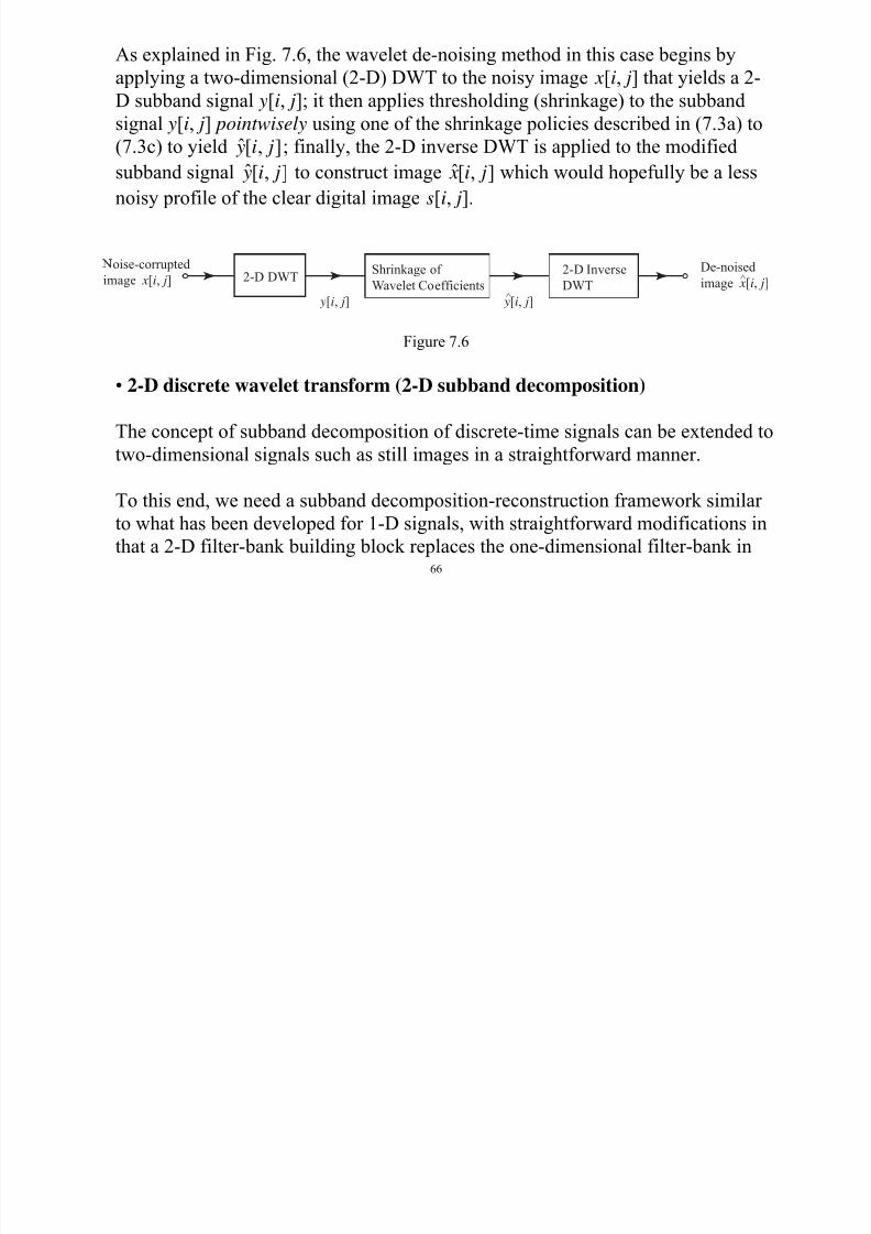
7/29/2019 Notes Wavelets
http://slidepdf.com/reader/full/notes-wavelets 66/74
66
D subband signal y[i, j]; it then applies thresholding (shrinkage) to the subband
signal y[i, j] pointwisely using one of the shrinkage policies described in (7.3a) to(7.3c) to yield ˆ[ , ] y i j ; finally, the 2-D inverse DWT is applied to the modified
subband signal ˆ[ , ] y i j to construct image ˆ[ , ] x i j which would hopefully be a less
noisy profile of the clear digital image s[i, j].
oise-corrupted
image x[i, j]
y[i, j] y[i, j]^
De-noised
image x[i, j]^2-D DWTShrinkage of
Wavelet Coefficients
2-D Inverse
DWT
Figure 7.6
• 2-D discrete wavelet transform (2-D subband decomposition)
The concept of subband decomposition of discrete-time signals can be extended to
two-dimensional signals such as still images in a straightforward manner.
To this end, we need a subband decomposition-reconstruction framework similar
to what has been developed for 1-D signals, with straightforward modifications in
that a 2-D filter-bank building block replaces the one-dimensional filter-bank in
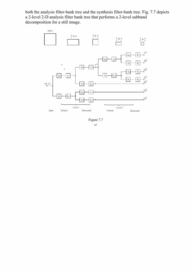
both the analysis filter-bank tree and the synthesis filter-bank tree. Fig. 7.7 depicts
a 2-level 2-D analysis filter bank tree that performs a 2-level subband
decomposition for a still image
7/29/2019 Notes Wavelets
http://slidepdf.com/reader/full/notes-wavelets 67/74
67
decomposition for a still image.
H0
H0
H0
H0
H0
H0
H1
H1
H1
H1
H1
H1
2
2
2
2
2
2
2
2
2
2
2
2
Level 1 Level 2
Input Vertical Horizontal Vertical Horizontal
a(2)
a(1)
d 01(2)
d 11(2)
d 10(2)
d 01(1)
d 11(1)
d 10(1)
{ x(i, j)}
N N
N 2
N 2
N 4
N 4
N 4
N 2
N 2
N
Figure 7.7
To illustrate how it works, let input signal { [ , ],0 1,0 1} x i j i N j N ≤ ≤ − ≤ ≤ −
represent an image of size N × N , where the value of x[i, j] is the gray scale of the
image pixel at position [i j] So it is of convenience to treat a digitized image as a
7/29/2019 Notes Wavelets
http://slidepdf.com/reader/full/notes-wavelets 68/74
68
image pixel at position [i, j]. So it is of convenience to treat a digitized image as a
matrix, just like a digitized 1-D signal is treated as a vector . At eachdecomposition level, we see a basic 2-D analysis filter bank that consists of 3 two-
channel 1-D filter banks, where the first 2-channel filter-bank filters and
downsamples the input image column by column. As a result, it outputs an
approximate image of size N /2 × N and a detail image of the same size. Then
each of these images is filtered by a 2-channel filter bank row by row, yielding 4
subimages of size N /2 × N /2 that are denoted as (1) (1) (1) (1)
01 10 11, , , and a d d d . This
completes the first-level 2-D subband decomposition. If necessary, the
approximation subimage a(1) can be further decomposed using the same filter
bank module described above to obtain subimages(2) (2) (2) (2)
01 10 11, , , and a d d d of size N /4 × N /4. Thus a two-level 2-D subband decomposition yields a total of 7
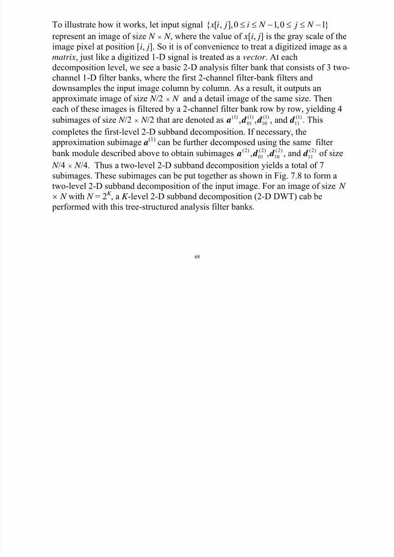
subimages. These subimages can be put together as shown in Fig. 7.8 to form a
two-level 2-D subband decomposition of the input image. For an image of size N
× N with N = 2K , a K -level 2-D subband decomposition (2-D DWT) cab be
performed with this tree-structured analysis filter banks.
a(2)d 01
(2)
d(1)
7/29/2019 Notes Wavelets
http://slidepdf.com/reader/full/notes-wavelets 69/74
69
d 11(2)d 10(2)
d 01( )
d 11(1)
d 10(1)
Figure 7.8
Also similar to the 1-D case, the 2-D inverse DWT can be performed using a tree-structure 2-D synthesis filter bank that is mirror-image symmetrical to the analysis
filter bank in Fig. 7.7, where the filters H0 and H1 are replaced with F0 and F1,
respectively, and the downsamplers are replaced by upsamplers. See Fig. 7.9 for a
two-level 2-D inverse DWT.
• Determination of threshold δ
Let the input image be of size N × N , Donoho’s universal threshold is then given
by
10ˆ2 log N δ σ = (7.7)
h2ˆ i ti t f th i i th t b bt i d i th
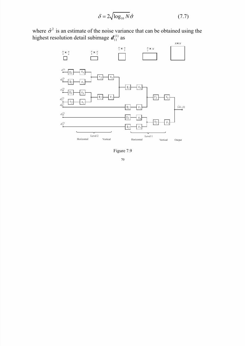
7/29/2019 Notes Wavelets
http://slidepdf.com/reader/full/notes-wavelets 70/74
70
where2
σ is an estimate of the noise variance that can be obtained using the
highest resolution detail subimage (1)11 d as
F0
F0
F0
F0
F0
F0
F1
F1
F1
F1
F1
F1
2
2
2
2
2
2
2
2
2
2
2
2
Level 1
Vertical OutputVertical Horizontal
Level 2
Horizontal
N N
N 2
N 2
N 4
N 4
N 4
N 2
N 2
N
a(2)
d 01(2)
d 11(2)
d 10(2)
d 01(1)
d 11
(1)
d 10(1)
{ x(i, j)}^
Figure 7.9
/ 2 / 22 (1) 2
1121 1
4ˆ [ ( , ) ]
4
N N
i j
d i j d N
σ = =
= −−
∑∑
7/29/2019 Notes Wavelets
http://slidepdf.com/reader/full/notes-wavelets 71/74
71
/ 2 / 2(1)
1121 1
4( , )
N N
i j
d d i j N = =
= ∑∑
(7.8)
Example 7.3 We now apply the above de-noising method with hyperbolicshrinkage and several wavelets to a 8-bit gray-scale image ‘fruits” of size 256 ×
256.
Noise:2
(0, )σ N with σ = 25.5953.
Wavelet: MIT 9/7
Shrinkage: HyperbolicThreshold: Universal
where the ‘MIT 9/7’ wavelet is characterized by a linear-phase lowpass analysis
filter H0 of length 9 and a linear-phase lowpass synthesis filter F0 of length 7
whose coefficients are given by
0
2[1 0 8 16 46 16 8 0 1]
64= − − h

7/29/2019 Notes Wavelets
http://slidepdf.com/reader/full/notes-wavelets 72/74
72
0
2[ 1 0 9 16 9 0 1]
32= − − f
For completeness, the highpass analysis and synthesis filters are characterized by
1
1
2[ 1 0 9 16 9 0 1]
32
2[ 1 0 8 16 46 16 8 0 1]
64
= − − −
= − − −
h
f
Results: The signal-to-noise ratio (SNR) before and after de-noising are given by
before 10
[ , ]SNR 20log 15.2327dB
[ , ] [ , ]F
F
s i j
x i j s i j= =
−
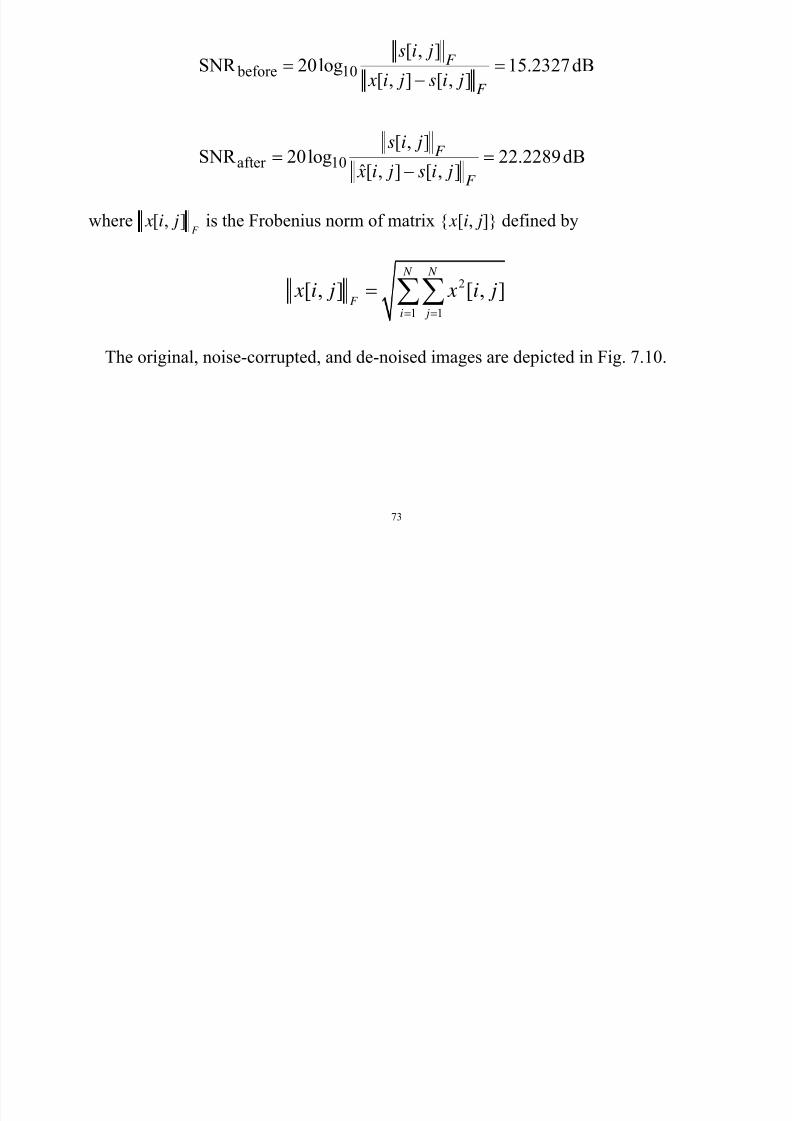
7/29/2019 Notes Wavelets
http://slidepdf.com/reader/full/notes-wavelets 73/74
73
after 10
[ , ]SNR 20log 22.2289dB
ˆ[ , ] [ , ]F
F
s i j
x i j s i j= =
−
where [ , ]F
x i j is the Frobenius norm of matrix { x[i, j]} defined by
2
1 1
[ , ] [ , ] N N
F i j
x i j x i j
= =
= ∑∑
The original, noise-corrupted, and de-noised images are depicted in Fig. 7.10.
origimal image noise−contaminated image
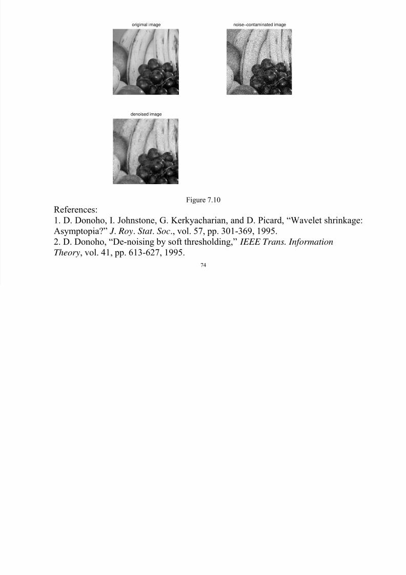
7/29/2019 Notes Wavelets
http://slidepdf.com/reader/full/notes-wavelets 74/74
74
denoised image
Figure 7.10
References:1. D. Donoho, I. Johnstone, G. Kerkyacharian, and D. Picard, “Wavelet shrinkage:
Asymptopia?” J . Roy. Stat . Soc., vol. 57, pp. 301-369, 1995.
2. D. Donoho, “De-noising by soft thresholding,” IEEE Trans. Information
Theory, vol. 41, pp. 613-627, 1995.