Mon. Not. R. Astron. Soc. 000, 1–19 (2015) Printed 3 February 2015 (MN LATEX style file v2.2)

Using the Inclinations of Kepler Systems to Prioritize NewTitius-Bode-Based Exoplanet Predictions

T. Bovaird1,2?, C. H. Lineweaver1,2,3 and S. K. Jacobsen41Research School of Astronomy and Astrophysics, Australian National University, Canberra, ACT 2611, Australia2Planetary Science Institute, Australian National University3Research School of Earth Sciences,Australian National University4Niels Bohr Institute, University of Copenhagen, Copenhagen, Denmark

3 February 2015

ABSTRACTWe analyze a sample of multiple-exoplanet systems which contain at least 3 transiting plan-ets detected by the Kepler mission (‘Kepler multiples’). We use a generalized Titius-Boderelation to predict the periods of 228 additional planets in 151 of these Kepler multiples.These Titius-Bode-based predictions suggest that there are, on average, 2±1 planets in thehabitable zone of each star. We estimate the inclination of the invariable plane for eachsystem and prioritize our planet predictions by their geometric probability to transit. Wehighlight a short list of 77 predicted planets in 40 systems with a high geometric probabilityto transit, resulting in an expected detection rate of ∼ 15 per cent, ∼ 3 times higher than thedetection rate of our previous Titius-Bode-based predictions.

Key words: exoplanets, Kepler, inclinations, Titius-Bode relation, multiple-planet systems,invariable plane

1 INTRODUCTION

The Titius-Bode (TB) relation’s successful prediction of the pe-riod of Uranus was the main motivation that led to the search foranother planet between Mars and Jupiter, e.g. Jaki (1972). Thissearch led to the discovery of the asteroid Ceres and the rest ofthe asteroid belt. The TB relation may also provide useful hintsabout the periods of as-yet-undetected planets around other stars.In Bovaird & Lineweaver (2013) (hereafter, BL13) we used a gen-eralized TB relation to analyze 68 multi-planet systems with fouror more detected exoplanets. We predicted the existence of 141new exoplanets in these 68 systems. Huang & Bakos (2014) (here-after, HB14) performed an extensive search in the Kepler data for97 of our predicted planets in 56 systems. This resulted in the con-firmation of 5 of our predictions. (Fig. 4 and Table 1).

In this paper we perform an improved TB analysis on a largersample of Kepler multiple-planet systems1 to make new exoplanetorbital period predictions. We use the expected coplanarity ofmultiple-planet systems to estimate the most likely inclination ofthe invariable plane of each system. We then prioritize our originaland new TB-based predictions according to their geometric prob-ability of transiting. Comparison of our original predictions withthe HB14 confirmations shows that restricting our predictions tothose with a high geometric probability to transit should increasethe detection rate by a factor of ∼ 3 (Fig. 8).

? E-mail: timothy.bovaird@anu.edu.au1 Accessed November 4th, 2014: http://exoplanetarchive.ipac.caltech.edu/cgi-bin/TblView/nph-tblView?app=ExoTbls&config=cumulative

As in BL13, our sample includes all Kepler multi-planet sys-tems with four or more exoplanets, but to these we add three-planetsystems if the orbital periods of the system’s planets adhere betterto the TB relation than the Solar System (Eq. 4 of BL13). Usingthese criteria we add 77 three-planet systems to the 74 systemswith four or more planets. We have excluded 3 systems: KOI-284,KOI-2248 and KOI-3444 because of concerns about false positivesdue to adjacent-planet period ratios close to 1 and close binaryhosts (Lissauer et al. 2011; Fabrycky et al. 2014; Lillo-Box et al.2014). We have also excluded the three-planet system KOI-593,since the period of KOI-593.03 was recently revised, excludingthe system from our three-planet sample. Thus, we analyze 151Kepler multiples, with each system containing 3, 4, 5 or 6 planets.

1.1 Coplanarity of exoplanet systems

Planets in the Solar System and in exoplanetary systems are be-lieved to form from protoplanetary disks (e.g. Winn & Fabrycky(2014)). The inclinations of the 8 planets of our Solar System tothe invariable plane are (in order from Mercury to Neptune) 6.3◦,2.2◦, 1.6◦, 1.7◦, 0.3◦, 0.9◦, 1.0◦, 0.7◦ (Souami & Souchay 2012).Jupiter and Saturn contribute ∼ 86 per cent of the total plane-tary angular momentum and thus the angles between their orbitalplanes and the invariable plane are small: 0.3◦ and 0.9◦ respec-tively.

In a given multiple-planet system, the distribution of mutualinclinations between the orbital planes of planets is well describedby a Rayleigh distribution (Lissauer et al. 2011; Fang & Margot2012; Figueira et al. 2012; Fabrycky et al. 2014; Ballard & John-

c© 2015 RAS

arX

iv:1

412.

6230

v3 [

astr

o-ph

.EP]

31

Jan

2015

2 T. Bovaird, C. H. Lineweaver and S. K. Jacobsen

θj

R*

ic

b

dj

0 2 4 6 8 10 12

2

1

0

1

Distance from host star [RO •]

R*/

RO •

⟨θ⟩

b)a)

To observer

j

To observer

z

y

x

z

θ⟨θ⟩

LL x

i

φ L

⟨L⟩⟨L⟩

jj

j

j

j∆θ

j

j

∆θj

Figure 1. Panel a): Our coordinate system for transiting exoplanets. The x-axis points towards the observer. ~Lj is the 3-D angular momentum of the jthplanet, and is perpendicular to the orbital plane of the jth planet. ~〈L〉 is the sum of the angular momenta of all detected planets (Eq. A2) and is perpendicularto the invariable plane of the system. We have chosen the coordinate system without loss of generality such that ~〈L〉 has no component in the y direction. φ j

is the angle between ~Lj and ~〈L〉. Let ~L j be the projection of ~Lj onto the x− z plane. ∆θ j is the angle between ~〈L〉 and ~L j . 〈θ〉 is the angle between the z axisand ~〈L〉. i j is the inclination of the planet (Eq. 3). θ j = 90− i j and is the angle between the z axis and ~L j such that θ j = 〈θ〉+∆θ j (Eq. A4). Panel b) showsthe x− z plane of Panel a) with the y axis pointing into the paper. The observer is to the right. The grey shaded region represents the ‘transit region’ wherethe centre of a planet will transit its host star as seen by the observer (impact parameter b 6 1, see Eq. 1). Four planets, b, c, d and j, are represented by bluedots. The intersection of the orbital plane of the jth planet with the x− z plane is shown (thin black line). All angles shown in Panel a) (with the exception ofφ j) are also shown in Panel b. The thick line is the intersection of the invariable plane of the system with the x− z plane. Because we are only dealing withsystems with multiple transiting planets, all these angles are typically less than a few degrees but are exaggerated here for clarity.

Kernel density estimate

Rayleigh 1°

Rayleigh 1.5°

0 1 2 3 4 5 6 7

0

1

2

Inclination to invariable plane φ

Nu

mber

of

pla

nets

Figure 2. The coplanarity of planets in the Solar System relative to theinvariable plane. With the exception of Mercury, the angles between theorbital planes of the planets and the invariable plane are well representedby a Rayleigh distribution with a mode of ∼ 1◦.

son 2014). For the ensemble of Kepler multi-planet systems, themode of the Rayleigh distribution of mutual inclinations (φ j−φi)is typically ∼ 1◦− 3◦ (Appendix A1 & Table A1). Thus, Keplermultiple-planet systems are highly coplanar. The Solar System issimilarly coplanar. For example, the mode of the best fit Rayleighdistribution of the planet inclinations (φ j) relative to the invariableplane in the Solar System is ∼ 1◦ (see Fig. 1 and 2)2.

The angle ∆θ j is a Gaussian distributed variable with a meanof 0 (centered around 〈θ〉) and standard deviation σ∆θ . Based onprevious analyses (Table A1), we assume the typical value σ∆θ =

2 See Appendix A for an explanation of why the distribution of mutualinclinations is on average a factor of

√2 wider than the distribution of the

angles φ j in Fig. 1, between the invariable plane of the system and theorbital planes of the planets.

1.5◦. We use this angle to determine the probability of detectingadditional transiting planets in each system.

Estimates of the inclination of a transiting planet come fromthe impact parameter b which is the projected distance betweenthe center of the planet at mid-transit and the center of the star, inunits of the star’s radius.

b =a

R∗cos i (1)

where R∗ is the radius of the star and a is the semi-major axis ofthe planet. For edge-on systems, typically 85◦ < i< 95◦. However,since we are unable to determine whether b is in the positive zdirection or the negative z direction (Fig.1b and Fig. B1), we areunable to determine whether i is greater than or less than 90◦. Byconvention, for transiting planets the sign of b is taken as positiveand thus the corresponding i values from Eq. 1 are taken as i6 90◦.

The impact parameter is also a function of four transit lightcurve observables (Seager & Mallén-Ornelas 2003); the period P,the transit depth ∆F , the total transit duration tT , and the total tran-sit duration minus the ingress and egress times tF (the durationwhere the light curve is flat for a source uniform across its disk).Thus the impact parameter can be written,

b = f (P,∆F, tT , tF ). (2)

Eliminating b from Eqs. (1) and (2) yields the inclination i as afunction of observables,

i = cos−1[

R∗a

f (P,∆F, tT , tF )]

(3)

From Eq. 1 we can see that for an impact parameter b = 0 (atransit through the center of the star), we obtain i = 90◦; an ‘edge-on’ transit.

The convention i 6 90◦ is unproblematic when only a singleplanet is found to transit a star but raises an issue when multipleexoplanets transit the same star, since the degree of coplanaritydepends on whether the actual values of i j ( j = 1,2, ..N where N

c© 2015 RAS, MNRAS 000, 1–19

Inclinations and Titius-Bode Predictions of Kepler Systems 3

is the number of planets in the system) are greater than or less than90◦. For example, the actual values of i j in a given system couldbe all > 90◦, all < 90◦ or some in-between combination. Althoughwe do not know the signs of θ j = 90◦− i j for individual planets,we can estimate the inclination of the invariable plane for eachsystem, by calculating all possible permutations of the θ j valuesfor each system (see Appendix A2). In this estimation, we use theplausible assumption that the coplanarity of a system should notdepend on the inclination of the invariable plane relative to theobserver.

1.2 The probability of additional transiting exoplanets

We wish to develop a measure of the likelihood of additionaltransiting planets in our sample of Kepler multi-planet systems.The more edge-on a planetary system is to an observer on Earth,the greater the probability of a planet transiting at larger periods.Similarly, a larger stellar radius leads to a higher probability ofadditional transiting planets (although with a reduced detectionefficiency). We quantify these tendencies under the assumptionthat Kepler multiples have a Gaussian opening angle σ∆θ = 1.5◦

around the invariable plane, and we introduce the variable, acrit.Planets with a semi-major axis greater than acrit have less than a50% geometric probability of transiting. More specifically, acrit isdefined as the semi-major axis where Ptrans(acrit) = 0.5 (Eq. B1)for a given system.

In a given system, a useful ratio for estimating the amountof semi-major axis space where additional transiting planets aremore likely, is acrit/aout, where aout is the semi-major axis of thedetected planet in the system which is the furthest from the hoststar. The larger acrit/aout, the larger the semi-major axis range foradditional transiting planets beyond the outermost detected planet.Values for this ratio less than 1 mean that the outermost detectedplanet is beyond the calculated acrit value, and imply that addi-tional transiting planets beyond the outermost detected planet areless likely. Figure 3 shows the acrit/aout distribution for all systemsin our sample. The fact that this distribution is roughly symmetricaround acrit/aout ∼ 1 strongly suggests that the outermost tran-siting planets in Kepler systems are due to the inclination of thesystem to the observer, and are not really the outermost planets.

In Section 2 we discuss the follow-up that has been done onour BL13 planet detections. In Section 3 we show that the ∼ 5%follow-up detection rate of HB14 is consistent with selection ef-fects and the existence of the predicted planets. In Section 4 weextend and upgrade the TB relation developed in BL13 and predictthe periods of undetected planets in our updated sample. We thenprioritize these predictions based on their geometric probability totransit and emphasize for further follow-up a subset of predictionswith high transit probabilities. We also use TB predictions to esti-mate the average number of planets in the circumstellar habitablezone. In Section 5 we discuss how our predicted planet insertionsaffect the period ratios of adjacent planets and explore how periodratios are tightly dispersed around the mean period ratio withineach system. In Section 6 we summarize our results.

2 FOLLOW-UP OF BL13 PREDICTIONS

BL13 used the approximately even logarithmic spacing of exo-planet systems to make predictions for the periods of 117 addi-tional candidate planets in 60 Kepler detected systems, and 24additional predictions in 8 systems detected via radial velocity(7)

Lessroom

More room for detections

0 1 2 3 4

0

10

20

30

40

acrit/aout

Nu

mber

of

syste

ms

Figure 3. Histogram of the acrit/aout values for our sample of Kepler mul-tiples. The distribution peaks for a ratio just below 1. Approximately halfof the systems lie to the right of 1. For these systems, if there are plan-ets with semi-major axes a such that aout < a < acrit then the geometricprobability of them transiting is greater than 50%. Note that this doesnot account for the detectability of these planets (e.g. they could be toosmall to detect). The majority of the predicted planets that are insertions(a < aout) have geometric transit probabilities greater than 50 per cent,when acrit/aout < 1. Systems on the right have more room for detections,and in general, predicted planets in these systems have higher values ofPtrans. The blue curve is the expected distribution of our sample of Keplermultiples if they all have planets at TB-predicted semi-major axes extrap-olated out to ∼ 4× acrit. The blue curve is consistent with the observeddistribution, indicating that our acrit/aout distribution is consistent with thesystem in our sample containing more planets than have been detected.

Table 1. Systems with candidate detections by HB14 (in bold) plusKOI-1151 (Petigura et al. 2013a) and KOI-1860 b, after planet pre-dictions were made by BL13.

System Predicted Detected Predicted DetectedPeriod (days) Period (days) Radius (R⊕) Radius (R⊕)

KOI-719 14±2 15.77 6 0.7 0.42KOI-1336 26±3 27.51 6 2.4 1.04KOI-1952 13±2 13.27 6 1.5 0.85KOI-2722a 16.8±1.0 16.53 6 1.6 1.16KOI-2859 5.2±0.3 5.43 6 0.8 0.76KOI-733 N/A 15.11 N/A 3.0KOI-1151a 9.6±0.7 10.43 6 0.8 0.7KOI-1860b 25±3 24.84 6 2.7 1.46

a Predicted by preprint of BL13 (draft uploaded 11 Apr 2013:http://arxiv.org/pdf/1304.3341v1.pdf), detected planet reported by Ke-pler archive and included in analysis of BL13.

b October 2014 Kepler Archive update, during the drafting of this paper.

and direct imaging(1), which we do not consider here. NASA Ex-oplanet Archive data updates, confirmed our prediction of KOI-2722.05 (Table 1).

HB14 used the planet predictions made in BL13 to search for97 planets in the light curves of 56 Kepler systems. Within these56 systems, BL13 predicted the period and maximum radius: thelargest radius which would have evaded detection, based on thelowest signal-to-noise of the detected planets in the same system.Predicted planets were searched for using the Kepler Quarter 1 toQuarter 15 long cadence light curves, giving a baseline exceeding1000 days. Once the transits of the already known planets were de-tected and removed, transit signals were visually inspected aroundthe predicted periods.

Of the 97 predicted planets searched for by HB14, 5 candi-dates were detected within ∼ one-sigma of the predicted periods

c© 2015 RAS, MNRAS 000, 1–19

4 T. Bovaird, C. H. Lineweaver and S. K. Jacobsen

KOI-719

KOI-1336

KOI-1952

KOI-2722

KOI-2859

KOI-733

KOI-1151

KOI-1860

0.0 0.1 0.2 0.3 0.4 0.5

0.0 0.1 0.2 0.3 0.4 0.5

Semi-Major Axis [AU]

Mercury

Earth

Uranus

Saturn

Figure 4. Exoplanet systems where an additional candidate was detected after a TB relation prediction was made (see Table 1). The systems are shown indescending order of acrit/aout. Previously known planets are shown as blue circles. The predictions of BL13 and their uncertainties are shown by the redfilled rectangles if the Ptrans value of the predicted planet is > 0.55 (Eq. B1 and Fig. 8), or by red hatched rectangles otherwise. The new candidate planetsare shown as green squares. The critical semi-major axis acrit (Section 1.2), beyond which Ptrans(acrit)< 0.5, is shown by a solid black arc. The uncertainties(width of red rectangles) in this figure and Table 1, are slightly wider than Figure 5 due to excessive rounding of predicted period uncertainties for somesystems in BL13.

KOI-719

KOI-1336

KOI-1952

KOI-2722

KOI-2859

KOI-733

KOI-1151

KOI-1860

0.0 0.1 0.2 0.3 0.4 0.5

0.0 0.1 0.2 0.3 0.4 0.5

Semi-Major Axis [AU]

Mercury

Earth

Uranus

Saturn

Figure 5. Same as Fig. 4 except here our TB predictions are based on γ with n2ins (Eq. 9) rather than on the γ with nins of Eq. 5 of BL13. Comparing Fig. 4

with this figure, in the KOI-719 system the number of predicted planets goes from 4 to 2, while in KOI-1151 the number of predicted planets goes from 3 to2. In both cases the detected planet is more centrally located in the predicted region.

c© 2015 RAS, MNRAS 000, 1–19

Inclinations and Titius-Bode Predictions of Kepler Systems 5

0 10 20 30 40 50 60 70

020406080

100

DSP

Kep

ler

SN

R

Figure 6. Reported dip significance parameter (DSP) from Table 1 ofHuang & Bakos (2014) for previously known exoplanets in the five sys-tems with a new detection. A linear trend can be seen for the DSP andthe signal-to-noise ratio as reported by the Kepler team (Christiansen et al.2012). HB14 required planet candidates to have a DSP > 8 to survive theirvetting process. The sizes of the blue dots correspond to the same planetaryradii representation used to make Figs. 11, 12, 13 & 14.

(5 planets of the 6 planets in bold in Table 1, see also Fig. 4). No-tably all new planet candidates have Earth-like or lower planetaryradii. One additional candidate was detected in KOI-733 whichis incompatible with the predictions of BL13. This candidate isunique in that it should have been detected previously, based onthe signal-to-noise of the other detected planets in KOI-733. InTable 1, the detected radii are less than the maximum predictedradii in each case. The new candidate in KOI-733 has a period of15.11 days and a radius of 3 R⊕. At this period, the maximum ra-dius to evade detection should have been 2.2 R⊕. With the possibleexception of KOI-1336 where a dip significance parameter (DSP,Kovács & Bakos (2005)) was not reported, all detected candidateshave a DSP of > 8, which roughly corresponds to a Kepler SNR(Christiansen et al. 2012) of & 12 (see Figure 6). HB14 requiredDSP > 8 for candidate transit signals to survive their vetting pro-cess.

3 IS A 5% DETECTION RATE CONSISTENT WITHSELECTION EFFECTS?

From a sample of 97 BL13 predictions, HB14 confirmed 5. How-ever, based on this ∼ 5% detection rate, HB14 concluded that thepredictive power of the TB relation used in BL13 was question-able. Given the selection effects, how high a detection rate shouldone expect? We do not expect all planet predictions to be detected.The predicted planets may have too large an inclination to tran-sit relative to the observer. Additionally, there is a completenessfactor due to the intrinsic noise of the stars, the size of the plan-ets, and the techniques for detection. This completeness for Ke-pler data has been estimated for the automated lightcurve analy-sis pipeline TERRA (Petigura et al. 2013a). Fig. 7 displays theTERRA pipeline injection/recovery completeness. After correct-ing for the radius and noise of each star, relative to the TERRAsample in Fig. 7, the planet detections in Table 1 have an averagedetection completeness in the TERRA pipeline of ∼ 24%. That is,if all of our predictions were correct and if all the planets were inapproximately the same region of period and radius space as thegreen squares in Fig. 7, and if all of the planets transited, we wouldexpect a detection rate of ∼ 24% using the TERRA pipeline. It isunclear how this translates into a detection rate for a manual inves-tigation of the lightcurves motivated by TB predictions.

We wish to determine, from coplanarity and detectability ar-guments, how many of our BL13 predictions we would have ex-pected to be detected. An absolute number of expected detectionsis most limited by the poorly known planetary radius distribution

5 10 20 30 40 50 100 200 300 400

Orbital period (days)

0.4

1

2

3

4

5

10

20

Pla

net s

ize

(Ear

th-r

adii)

0 10 20 30 40 50 60 70 80 90 100

Survey Completeness (C) %

Figure 7. The simulated detection completeness of the new candidate plan-ets in the TERRA pipeline (modified from Figure 1 of Petigura et al.(2013a)). Here we overplot as green squares, the 8 planets listed in Table 1.The completeness curves are averaged over all stellar noise and stellar radiiin the Petigura et al. (2013a) sample (the 42,000 least noisy Kepler stars).Green circles indicate the ‘effective radius’ of the new candidates, basedon the noise and radius of their host star in comparison to the median of thequietest 42,000 sample. From the signal-to-noise, the effective radius canbe calculated by Rp,eff/Rp = (R∗/R∗,median)× (CDPP/CDPPmedian)

1/2,where CDPP is the combined differential photometric precision definedin Christiansen et al. (2012). Taking a subset of 42,000 stars from the Ke-pler input catalog with the lowest 3-hour CDPP (approximately represen-tative of the sample in the figure), we obtain CDPPmedian ≈ 60 ppm andR∗,median ≈ 1.15 R�. Using the effective radius and excluding the outlierKOI-733, the mean detection completeness for the 7 candidate planets inTable 1 is ∼ 24%.

below 1 Earth radius (Howard et al. 2012; Dressing & Charbon-neau 2013; Dong & Zhu 2013; Petigura et al. 2013b; Fressin et al.2013; Silburt et al. 2014; Morton & Swift 2014; Foreman-Mackeyet al. 2014). Large uncertainties about the shape and amplitude ofthe planetary radius distribution of rocky planets with radii lessthan 1 Earth radius make the evaluation of TB-based exoplanetpredictions difficult. Since the TB relation predicted the asteroidbelt (Masteroid < 10−3MEarth) there seems to be no lower masslimit to the objects that the TB relation can predict. This makesestimation of the detection efficiencies strongly dependent on as-sumptions about the frequency of planets at small radii.

Let the probability of detecting a planet, Pdetect, be the productof the geometric probability to transit Ptrans as seen by the observer(Appendix B) and the probability PSNR that the planetary radius islarge enough to produce a signal-to-noise ratio above the detectionthreshold,

Pdetect = Ptrans PSNR. (4)

The geometric probability to transit, Ptrans, is defined in Eq.B1 and illustrated in Fig. 1 and Fig. B1. The 5 confirmations fromour previous TB predictions are found in systems with a muchhigher than random probability of transit (Fig. 8). This is expectedif our estimates of the invariable plane are reasonable.

To estimate PSNR we first estimate the probability that theradius of the planet will be large enough to detect. In BL13 we

c© 2015 RAS, MNRAS 000, 1–19

6 T. Bovaird, C. H. Lineweaver and S. K. Jacobsen

0.0 0.2 0.4 0.6 0.8 1.0

0

5

10

15

20

0%

20%

40%

60%

80%

100%

Ptrans

Nu

mber

of

pre

dic

ted p

lan

ets

Figure 8. Histogram of Ptrans (Eq. B1), the geometric probability of transit,for the 97 predicted planets from BL13, that were followed up by HB14.The blue histogram represents the 5 new planets detected by HB14 (Ta-ble 1). As expected, the detected planets have high Ptrans values comparedto the entire sample. The red and blue solid lines represent the empiricalcumulative distribution function for the two distributions. A K-S test of thetwo distributions yields a p-value of 1.8×10−2. Thus, Ptrans can be used toprioritize our predictions and increase their probability of detection.

MarsMercury

Rlow Rmax

-0.5 0.0 0.5 1.0 1.5 1 10

Log planet radius [R⊕]

0.0

0.2

0.4

0.6

0.8

f (R)

undetectable detectable already detected already detected

Rel

ativ

e fr

equ

ency

?

0.1

-1.0

Rmin

Ceres

Figure 9. The assumed distribution of planetary radii described in Sec-tion 3. The distribution is poorly constrained below 1 Earth radii, indicatedby the gray dashed line. For low mass stars, the planetary radius distribu-tion may decline below 0.7 R⊕ (Dressing & Charbonneau 2013; Morton &Swift 2014). Alternative estimations show the planetary radius distributioncontinuing to increase with smaller radii (continuing the flat logarithmicdistribution), down to 0.5 R⊕ (Foreman-Mackey et al. 2014). For our anal-ysis we have extrapolated the flat distribution (in log R) down to Rlow. Weindicate three regions for a hypothetical system at a specific predicted pe-riod. The ‘already detected’ region refers to the range of planetary radiiwhich should already have been detected, based on the lowest signal-to-noise ratio of the detected planets in that system. Rmin is the smallest radiuswhich could produce a transit signal that exceeds the detection threshold,and is the boundary between the undetectable and detectable regions.

estimated the maximum planetary radius, Rmax, for a hypotheticalundetected planet at a given period, based on the lowest signal-to-noise of the detected planets in the same system. We now wishto estimate a minimum radius that would be detectable, given theindividual noise of each star. We refer to this parameter as Rmin,which is the minimum planetary radius that Kepler could detectaround a given star (using a specific SNR threshold). For each starwe used the mean CDPP (combined differential photometric pre-cision) noise from Q1-Q16. When the number of transits is notreported, we use the approximation Ntrans ≈ Tobs f0/P, where Tobsis the total observing time and f0 is the fractional observing up-time, estimated at∼0.92 for the Kepler mission (Christiansen et al.2012).

The probability PSNR depends on the underlying planetary ra-dius probability density function. We assume a density function of

7 8 9 10 11 12 13 14 15

0.1

0.2

0.3

0.4

0.50.6

5%

10%

15%

20%

25%5 6 7 8 9

Transit SNR threshold

Rlo

w [R

⊕]

Transit DSP thresholdP detect

5%

10%

15%

20%

3%

HB14

Figure 10. The mean detection rate Pdetect (Eq. 4) of the BL13 predictionsis dependent on the transit signal-to-noise threshold (SNRth in Eq. 8) usedin lightcurve vetting (x-axis), and on the probability of low-radii planets,i.e. on how far the flat logarithmic planetary radius distribution in Fig. 9should be extrapolated (Rlow on the y-axis). For example, in the denomi-nator of Eq. 6, integrating down to a radius Rlow of 0.6 R⊕ and setting aSNR threshold of 7 (which sets Rmin in the numerator) gives an expecteddetection fraction of∼ 25% (blue values in the upper left of the plot). Inte-grating down to a radius of 0.2 R⊕ and having a DSP threshold of 8 (con-verted from SNR according to Fig. 6) gives an expected detection fractionof ∼ 5% (red values in the lower right).

the form:

f (R) =d f

dlogR=

{k(logR)α , R > 2.8 R⊕k(log2.8)α , R < 2.8 R⊕

(5)

where k = 2.9 and α = −1.92 (Howard et al. 2012). The dis-continuous distribution accounts for the approximately flat num-ber of planets per star in logarithmic planetary radius bins forR . 2.8 R⊕ (Dong & Zhu 2013; Fressin et al. 2013; Petiguraet al. 2013b; Silburt et al. 2014). For R . 1.0 R⊕ the distributionis poorly constrained. For this paper, we extend the flat distribu-tion in log R down to a minimum radius Rlow = 0.3 R⊕. It is im-portant to note that for the Solar System, the poorly constrainedpart of the planetary radius distribution contains 50 per cent of theplanet population. For reference the radius of Ceres, a “planet”predicted by the TB relation applied to our Solar System has aradius RCeres = 476 km = 0.07R⊕.

The probability that the hypothetical planet has a radius thatexceeds the SNR detection threshold is then given by

PSNR =

∫ RmaxRmin

f (R)dR∫ RmaxRlow

f (R)dR(6)

We do not integrate beyond Rmax since we expect a planet witha radius greater than Rmax would have already been detected. Wedefine Rmax by,

Rmax = Rmin SNR

(Ppredict

Pmin SNR

)1/4, (7)

where Rmin SNR and Pmin SNR are the radius and period respectivelyof the detected planet with the lowest signal-to-noise in the system.Ppredict is the period of the predicted planet. Rmin depends on theSNR in the following way:

Rmin = R∗√

SNRth CDPP(

3hrsntr tT

)1/4, (8)

where SNRth is the SNR threshold for a planet detection, ntr isthe number of expected transits at the given period and tT is the

c© 2015 RAS, MNRAS 000, 1–19

Inclinations and Titius-Bode Predictions of Kepler Systems 7

transit duration in hours. See Figure 9 for an illustration of howthe integrals in PSNR (Eq. 6) depend on the planet radii limits, Rminand Rlow.

While Ptrans is well defined, PSNR is dependent on the SNRthreshold chosen (SNRth), the choice of Rlow and the poorly con-strained shape of the planetary radius distribution below 1 Earthradius. This is demonstrated in Figure 10, where the mean Pdetectfrom the predictions of BL13 (for DSP > 8) can vary from ∼ 2per cent to ∼ 11 per cent. Performing a K-S test on PSNR values(analogous to that in Figure 8) indicates that the PSNR values forthe subset of our BL13 predictions that were detected, are drawnfrom the same PSNR distribution as all of the predicted planets. Forthis reason we use only Ptrans, the geometric probability to tran-sit, to prioritize our new TB relation predictions. We emphasize asubset of our predictions which have a Ptrans value > 0.55, sinceall of the confirmed predictions of BL13 had a Ptrans value abovethis threshold. Only ∼ 1/3 of the entire sample have Ptrans valuesthis high. Thus, the ∼ 5 per cent detection rate should increase bya factor of ∼ 3 to ∼ 15 per cent for our new high-Ptrans subset ofplanet period predictions.

4 UPDATED PLANET PREDICTIONS

4.1 Method and Inclination Prioritization

We now make updated and new TB relation predictions in all151 systems in our sample. If the detected planets in a systemadhere to the TB relation better than the Solar System planets(χ2/d.o.f.< 1.0, Equation 4 of BL13), we only predict an extrapo-lated planet, beyond the outermost detected planet. If the detectedplanets adhere worse than the Solar System, we simulate the in-sertion of up to 9 hypothetical planets into the system, covering allpossible locations and combinations, and calculate a new χ2/d.o.f.value for each possibility. We determine how many planets to in-sert, and where to insert them, based on the solution which im-proves the system’s adherence to the TB relation, scaled by thenumber of inserted planets squared. This protects against overfit-ting (inserting too many planets, resulting in too good a fit). In Eq.5 of BL13 we introduced a parameter γ , which is a measure of thefractional amount by which the χ2/d.o.f. improves, divided by thenumber of planets inserted. Here, we improve the definition of γ

by dividing by the square of the number of planets inserted,

γ =

(χ2

i −χ2f

χ2f

)n2

ins(9)

where χ2i and χ2

f are the χ2 of the TB relation fit before and af-ter planets are inserted respectively, while nins is the number ofinserted planets.

Importantly, when we calculate our γ value by dividing bythe number of inserted planets squared, rather than the numberof planets, we still predict the BL13 predictions that have beendetected. In two of these systems fewer planets are predicted andas a result the new predictions agree better with the location of thedetected candidates. This can be seen by comparing Figures 4 and5.

We compute Ptrans for each planet prediction in our sampleof 151 Kepler systems. We emphasize the 40 systems where atleast one inserted planet in that system has Ptrans > 0.55. Periodpredictions for this subset of 40 systems are displayed in Table C1and Figures 11, 12 and 13. As discussed in the previous section,we expect a detection rate of ∼ 15 per cent for this high-Ptrans

sample. Predictions for all 228 planets (regardless of their Ptransvalue) are shown in Table C2 (where the systems are ordered bythe maximum Ptrans value in each system).

4.2 Average Number of Planets in Circumstellar HabitableZones

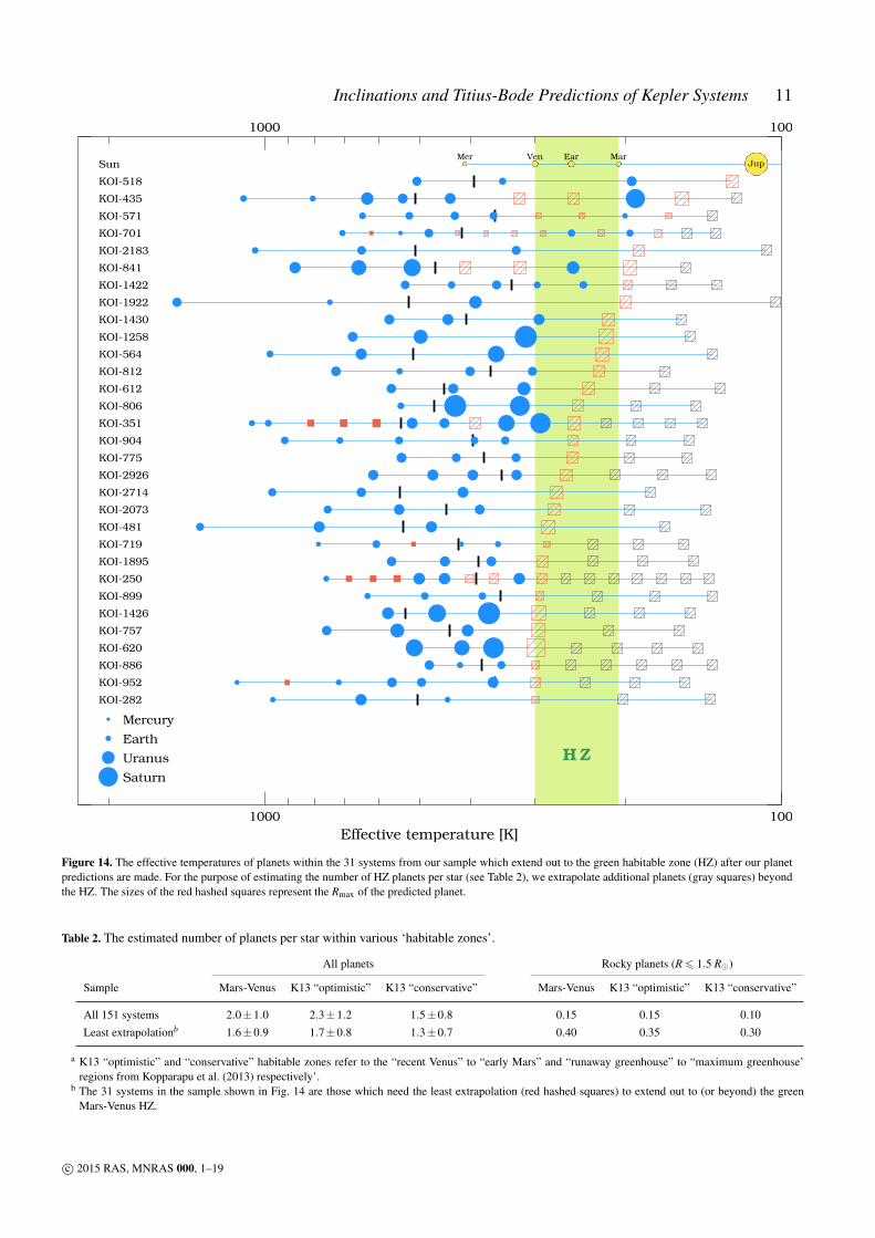
Since the search for earth-sized rocky planets in circumstellar hab-itable zones (HZ) is of particular importance, in Fig. 14, for asubset of Kepler multiples whose predicted (extrapolated) planetsextend to the HZ, we have converted the semi-major axes of de-tected and predicted planets into effective temperatures (as in Fig.6 of BL13). One can see in Fig. 14 that the habitable zone (shadedgreen) contains between 0 and 4 planets. Thus, if the TB relation isapproximately correct, and if Kepler multi-panet systems are rep-resentative of planetary systems in general, there are on average∼ 2 habitable zone planets per star.

More specifically, in Table 2, we estimate the number of plan-ets per star in various ‘habitable zones’, namely (1) the range ofTeff between Mars and Venus (assuming an albedo of 0.3), dis-played in Fig.14 as the green shaded region, (2) the Kopparapuet al. (2013) “optimistic” and (3) “conservative” habitable zones(“recent Venus” to “early Mars”, and “runaway greenhouse” to“maximum greenhouse” respectively). We find, on average, 2± 1planets per star in the “habitable zone”, almost independently ofwhich of the 3 habitable zones one is referring to. Using our es-timates of the maximum radii for these predominantly undetected(but predicted) planets, as well as the planetary radius distribu-tion of Fig. 9, we estimate that on average, ∼ 1/6 of these ∼ 2planets, or ∼ 0.3, are ‘rocky’. We have assumed that planets withR 6 1.5R⊕ are rocky (Rogers 2014; Wolfgang & Lopez 2014).

5 ADJACENT PLANET PERIOD RATIOS

HB14 concluded that the percentage of detected planets (∼ 5%)was on the lower side of their expected range (∼ 5%− 20%) andthat the TB relation may over-predict planet pairs near the 3:2mean-motion resonance (compared to systems which adhered tothe TB relation better than the Solar System, without any planetinsertions. i.e. χ2/d.o.f 6 1). There is some evidence that a peakin the distribution of period ratios around the 3:2 resonance is tobe expected from Kepler data, after correcting for incompletenessSteffen & Hwang (2014). In this section we investigate the periodratios of adjacent planets in our Kepler multiples before and afterour new TB relation predictions are made.

We divide our sample of Kepler multiples into a number ofsubsets. Our first subset includes systems which adhere to the TBrelation better than the Solar System (where we only predict an ex-trapolated planet beyond the outermost detected planet). Systemswhich adhere to the TB relation worse than the Solar System wedivide into two subsets, before and after the planets predicted bythe TB relation were inserted. Adjacent planet period ratios can bemisleading if there is an undiscovered planet between two detectedplanets, which would reduce the period ratios if it was includedin the data. To minimize this incompleteness, we also construct asubset of systems which are the most likely to be completely sam-pled (unlikely to contain any additional transiting planets withinthe range of the detected planet periods).

Systems which adhere to the TB relation better than the SolarSystem (χ2/d.o.f6 1) were considered by HB14 as being the sam-ple of planetary systems that were most complete and therefore

c© 2015 RAS, MNRAS 000, 1–19

8 T. Bovaird, C. H. Lineweaver and S. K. Jacobsen

⟨θ⟩

0.4KOI-1198

0.8

KOI-1955

0.6KOI-1082

0.5KOI-952

1.6

KOI-500

2.7

KOI-4032

1.2

KOI-707

1.0

KOI-1336

4.1

KOI-2859

0.3KOI-250

0.3KOI-168

0.5KOI-2585

0.3KOI-1052

1.3

KOI-505

0.0 0.1 0.2 0.3 0.4 0.5

0.0 0.1 0.2 0.3 0.4 0.5

Semi-Major Axis [AU]

Mercury

Earth

Uranus

Saturn

Figure 11. The architectures and invariable plane inclinations for Kepler systems in our sample which contain at least one planet with a geometric probabilityto transit Ptrans > 0.55. There are 40 such systems out of the 151 in our sample. The 14 with the highest Ptrans values are plotted here. The remaining 26 areplotted in the next two figures. The order of the systems (from top to bottom) is determined by the highest Ptrans value in each system. The thin horizontaldotted line represents the line-of-sight to Earth, i.e. where the i value of a planet would be 90◦. The thick grey line in each system is our estimate of theinvariant plane angle, 〈θ〉 (Appendix A2). The value of 〈θ〉 is given in degrees to the right of each panel (see also Fig. A1). The green wedge has an openingangle σ∆θ = 1.5◦ and is symmetric around the invariable plane, but is also limited to the grey region where a planet can be seen to transit from Earth (b 6 1,Eq. 1). The thick black arc indicates the acrit value beyond which less than 50 per cent of planets will transit (Eq. B1). Predicted planets and their uncertaintiesare shown by solid red rectangles if the Ptrans value of the predicted planet is > 0.55, or by red hatched rectangles otherwise. Thus, the 77 solid red rectanglesin the 40 systems shown in Figs. 11,12 & 13 make up our short list of highest priority predictions (Table C1). Our estimate of the most probable inclinationambiguities in a system are represented by vertically separated pairs of blue dots, connected by a thin black line (see Appendix A2).

c© 2015 RAS, MNRAS 000, 1–19

Inclinations and Titius-Bode Predictions of Kepler Systems 9

⟨θ⟩

0.3KOI-1831

1.5

KOI-248

0.3KOI-880

0.3KOI-1567

0.8

KOI-1952

0.0KOI-351

0.2KOI-701

0.3KOI-1306

0.5KOI-2722

0.4KOI-1358

0.5KOI-1627

0.8

KOI-1833

0.7KOI-3158

1.2

KOI-2055

0.5KOI-245

1.5

KOI-749

0.0 0.1 0.2 0.3 0.4 0.5

0.0 0.1 0.2 0.3 0.4 0.5

Semi-Major Axis [AU]

Mercury

Earth

Uranus

Saturn

Figure 12. The same as Figure 11 but for the next 16 systems in our sample which have at least one planet with Ptrans > 0.55. Note that some of the newdetected planets from the predictions of BL13 have been included in the Kepler data archive (see Table 1), and that these planets are included in our analysis.

c© 2015 RAS, MNRAS 000, 1–19

10 T. Bovaird, C. H. Lineweaver and S. K. Jacobsen

⟨θ⟩

0.3KOI-730

0.6KOI-719

0.4KOI-1060

1.6

KOI-3083

0.8KOI-156

0.7KOI-137

0.5KOI-1151

0.3KOI-1015

0.8KOI-2029

1.1

KOI-664

0.0 0.1 0.2 0.3 0.4 0.5

0.0 0.1 0.2 0.3 0.4 0.5

Semi-Major Axis [AU]

Mercury

Earth

Uranus

Saturn

Figure 13. The same as Figures 11 & 12 but for the remaining 10 systems in our sample which have at least one planet with Ptrans > 0.55.

had a distribution of adjacent planet period ratios most representa-tive of actual planetary systems. However, the choice of BL13 tonormalize the TB relation to the Solar System’s χ2/d.o.f is some-what arbitrary. The Solar System’s χ2/d.o.f is possibly too high toconsider all those with smaller values of χ2/d.o.f to be completelysampled.

We want to find a set of systems which are unlikely to hostany additional planets between adjacent pairs, due to the systembeing dynamically full (Hayes & Tremaine 1998). We do this byidentifying the systems where two or more sequential planet pairsare likely to be unstable when a massless test particle is insertedbetween each planet pair (dynamical spacing ∆ < 10, Gladman(1993), BL13).

The dynamical spacing ∆ is an estimate of the stability of ad-jacent planets. If inserting a test particle between a detected planetpair results in either of the two new ∆ values being less than 10,we consider the planet pair without the insertion to be complete.That is, there is unlikely to be room, between the detected planetpair, where an undetected planet could exist without making theplanet pair dynamically unstable. Therefore, since the existence ofan undetected planet between the planet pair is unlikely, we refer to

the planet pair as ‘completely sampled’. Estimating completenessbased on whether a system is dynamically full is a reasonable ap-proach, since there is some evidence that the majority of systemsare dynamically full (e.g. Barnes & Raymond (2004)). For Ke-pler systems in particular, Fang & Margot (2013) concluded thatat least 45 per cent of 4-planet Kepler systems are dynamicallypacked.

If at least two sequential adjacent-planet pairs (at least threesequential planets) satisfy this criteria, we add the subset of thesystem which satisfies this criteria to our ‘most complete’ sam-ple. We use this sample to analyze the period ratios of Kepler sys-tems. The period ratios of the different samples described aboveare shown in Figure 15.

One criticism from HB14 was that the TB relation from BL13inserted too many planets. To address this criticism we have rede-fined γ to be divided by the number of inserted planets squared(denominator of Eq. 9). This introduces a heavier penalty for in-serting planets. Figure 15 displays the distributions of period ratioswhen using the γ from BL13 and the new γ of Equation 9 (panelsb and c respectively). When using our newly defined γ , the mean

c© 2015 RAS, MNRAS 000, 1–19

Inclinations and Titius-Bode Predictions of Kepler Systems 11

Mer Ven Ear Mar

JupSun

KOI-518

KOI-435

KOI-571

KOI-701

KOI-2183

KOI-841

KOI-1422

KOI-1922

KOI-1430

KOI-1258

KOI-564

KOI-812

KOI-612

KOI-806

KOI-351

KOI-904

KOI-775

KOI-2926

KOI-2714

KOI-2073

KOI-481

KOI-719

KOI-1895

KOI-250

KOI-899

KOI-1426

KOI-757

KOI-620

KOI-886

KOI-952

KOI-282

1000 100

1000 100

Effective temperature [K]

H Z

Mercury

Earth

Uranus

Saturn

Figure 14. The effective temperatures of planets within the 31 systems from our sample which extend out to the green habitable zone (HZ) after our planetpredictions are made. For the purpose of estimating the number of HZ planets per star (see Table 2), we extrapolate additional planets (gray squares) beyondthe HZ. The sizes of the red hashed squares represent the Rmax of the predicted planet.

Table 2. The estimated number of planets per star within various ‘habitable zones’.

All planets Rocky planets (R 6 1.5 R⊕)

Sample Mars-Venus K13 “optimistic” K13 “conservative” Mars-Venus K13 “optimistic” K13 “conservative”

All 151 systems 2.0±1.0 2.3±1.2 1.5±0.8 0.15 0.15 0.10Least extrapolationb 1.6±0.9 1.7±0.8 1.3±0.7 0.40 0.35 0.30

a K13 “optimistic” and “conservative” habitable zones refer to the “recent Venus” to “early Mars” and “runaway greenhouse” to “maximum greenhouse’regions from Kopparapu et al. (2013) respectively’.

b The 31 systems in the sample shown in Fig. 14 are those which need the least extrapolation (red hashed squares) to extend out to (or beyond) the greenMars-Venus HZ.

c© 2015 RAS, MNRAS 000, 1–19

12 T. Bovaird, C. H. Lineweaver and S. K. Jacobsen

5:22:15:33:24:35:4

Adheres to TBR better

than Solar System

(χ2/d.o.f. < 1.0):

Mean

χ2/d.o.f.

= 0.48

0

5

10

15

N

a)

Adheres to TBR worse

than Solar System:

after insertions0.27γ ∝ nins

-1

0

5

10

15

N

b)

Adheres to TBR worse

than Solar System:

after insertions0.36γ ∝ nins

-2

0

5

10

15

N

c)

Adheres to TBR worse

than Solar System:

before insertions3.16

02

4

6

8

N

d)

’Most complete’ sample:

Pairs with ∆ < 10 (after

insertion of 1 M⊕

planet between pair)

0.40

1 2 3 4

02

4

6

8

Pouter/Pinner

N

e)

Figure 15. The period ratios of adjacent-planet pairs in our sample of Ke-pler multiples, which can be compared to Figure 4 of HB14. Panel a) repre-sents systems which adhere to the TB relation better than the Solar System(χ2/d.o.f. < 1). Panel b) represents those systems which adhere to the TBrelation worse than the Solar System and where BL13 inserted planets.This panel shows the period ratios of adjacent-planet pairs after planetsare inserted. Panel c) is similar to Panel b), except that the γ value, whichis used to determine the best TB relation insertion for a given system, isdivided by the number of inserted planets squared. In BL13 and panel b),γ was divided by the number of inserted planets. Panel d) shows the pe-riod ratios between adjacent pairs of the same systems from panels b) andc), except before the additional planets from the predictions of BL13 havebeen inserted. Panel e) represents our most complete sample and containsthe systems which are more likely to be dynamically full (as defined inSection 5). The mean χ2/d.o.f. value for each subset is shown on the leftside of each panel. Kepler’s bias toward detecting compact systems domi-nated by short period planets may explain why the Solar System’s adjacentperiod pairs (black hatched histogram in panel e) are not representative ofthe histogram in panel e. The periods of predicted planets are drawn ran-domly from their TB relation predicted Gaussian distributions (Tables C1and C2).

χ2/d.o.f. (displayed on the left side of the panels), more closelyresembles that of our ‘most complete sample’ (panel e).

Since each panel in Fig. 15 represents a mixture of planetarysystems with different distributions of period ratios, Figure 16 maybe a better way to compare these different samples and their adher-ence to the TB relation. For each planetary system in each panel inFig. 15, we compute the mean adjacent-planet period ratio. Figure16 shows the distribution of the offsets from the mean period ratioof each system. How peaked a distribution is, is a good measure ofhow well that distribution adheres to the TB relation. A delta func-tion peak at an offset of zero, would be a perfect fit. The periodratios of adjacent-planet pairs in our dynamically full “most com-plete sample” (green in Fig. 16) displays a significant tendency tocluster around the mean ratios. This clustering is the origin of theusefulness of the TB relation to predict the existence of undetectedplanets. The proximity of the thick blue curve to the green distri-bution is a measure of how well our TB predictions can correct for

-1.0 -0.5 0.0 0.5 1.00.00

0.05

0.10

0.15

Offset from mean period ratio

Rel

ativ

e fr

equ

ency

Figure 16. Each system has a mean value for the adjacent-planet periodratios within that system. This figure shows the distribution of the periodratios, offset from the mean period ratio of the system. The colors of thedistributions correspond to subsets in Figure 15. The green distribution isfrom the ‘most complete sample’ in panel e) and is our best estimate ofwhat a distribution should look like if an appropriate number of planetshave been inserted. The gray distribution indicates that the sampling ofthese systems is highly incomplete. The thick and thin blue lines repre-sent panel c) in two different ways. The thick blue line uses planet peri-ods drawn randomly from a normal distribution centered on the periodspredicted by the TB relation, with the width set to the uncertainty in theperiod predictions (Tables C1 and C2). The thin blue line uses periods attheir exact predicted value.

the incompleteness in Kepler multiple-planet systems and makepredictions about the probable locations of the undetected planets.

6 CONCLUSION

Huang & Bakos (2014) investigated the TB relation planet predic-tions of Bovaird & Lineweaver (2013) and found a detection rateof ∼ 5% (5 detections from 97 predictions). Apart from the detec-tions by HB14, only one additional planet (in KOI-1151) has beendiscovered in any of the 60 Kepler systems analyzed by BL13 –indicating the advantages of such predictions while searching fornew planets. Completeness is an important issue (e.g. Figures 7 &10). Some large fraction of our predictions will not be detected be-cause the planets in this fraction are likely to be too small to pro-duce signal-to-noise ratios above some chosen detection thresh-old. Additionally, the predicted planets may have inclinations andsemi-major axes too large to transit their star as seen from Earth.All new candidate detections based on the predictions of BL13 areapproximately Earth-sized or smaller (Table 1).

For a new sample of Kepler multiple-exoplanet systems con-taining at least three planets, we computed invariable plane incli-nations and assumed a Gaussian opening angle of coplanarity ofσ∆θ = 1.5◦. For each of these systems we applied an updated gen-eralized TB relation, developed in BL13, resulting in 228 predic-tions in 151 systems.

We emphasize the planet predictions which have a high geo-metric probability to transit, Ptrans > 0.55 (Figure 8). This subsetof predictions has 77 predicted planets in 40 systems. We expectthe detection rate in this subset to be a factor of∼ 3 higher than thedetection rate of the BL13 predictions. From the 40 systems withplanet predictions in this sample, 24 appeared in BL13. These pre-dictions have been updated and reprioritized. We have ordered ourlist of predicted planets based on each planet’s geometric prob-ability to transit (Tables C1 and C2). Our new prioritized predic-tions should help on-going planet detection efforts in Kepler multi-planet systems.

c© 2015 RAS, MNRAS 000, 1–19

Inclinations and Titius-Bode Predictions of Kepler Systems 13

ACKNOWLEDGEMENTS

T.B. acknowledges support from an Australian PostgraduateAward. We acknowledge useful discussions with Daniel Bayliss,Michael Ireland, George Zhou and David Nataf.

REFERENCES

Ballard S., Johnson J. A., 2014, ApJ (submitted), arXiv:1410.4192Barnes R., Raymond S. N., 2004, ApJ, 617, 569, doi:10.1086/423419Bovaird T., Lineweaver C. H., 2013, MNRAS, 435, 1126Christiansen J. L. et al., 2012, PASP, 124, 1279Dong S., Zhu Z., 2013, ApJ, 778, 53, doi:10.1088/0004-637X/778/1/53Dressing C. D., Charbonneau D., 2013, ApJ, 767, 95, doi:10.1088/0004-

637X/767/1/95Fabrycky D. C., Winn J. N., 2009, ApJ, 696, 1230Fabrycky D. C. et al., 2014, ApJ, 790, 146Fang J., Margot J.-L., 2012, ApJ, 761, 92Fang J., Margot J.-L., 2013, ApJ, 767, 115Figueira P. et al., 2012, A&A, 541, A139Foreman-Mackey D., Hogg D. W., Morton T. D., . 2014, ApJ, 795, 64,

doi:10.1088/0004-637X/795/1/64Fressin F. et al., 2013, ApJ, 766, 81Gladman B., 1993, Icarus, 106, 247Hayes W., Tremaine S., 1998, Icarus, 135, 549,

doi:10.1006/icar.1998.5999Howard A. W. et al., 2012, ApJS, 201, 15Huang C. X., Bakos G. A., 2014, MNRAS, 681, 674Jaki S. L., 1972, Am. J. Phys., 40, 1014Johansen A., Davies M. B., Church R. P., Holmelin V., 2012, ApJ, 758,

39, doi:10.1088/0004-637X/758/1/39Kopparapu R. K. et al., 2013, ApJ, 765, 131, doi:10.1088/0004-

637X/765/2/131Kovács G., Bakos G., 2005, arXiv:0508081Lillo-Box J., Barrado D., Bouy H., . 2014, A&A, 556, A103Lissauer J. J. et al., 2011, ApJS, 197, 8Morton T. D., Swift J., 2014, ApJ, 791, 10, doi:10.1088/0004-

637X/791/1/10Petigura E. A., Howard A. W., Marcy G. W., . 2013a, PNAS, 110, 19273Petigura E. A., Marcy G. W., Howard A., . 2013b, ApJ, 770, 69Rogers L. a., 2014, ApJ (submitted), arXiv:1407.4457Seager S., Mallén-Ornelas G., 2003, ApJ, 585, 1038Silburt A., Gaidos E., Wu Y., . 2014, preprint (arXiv:1406.6048v2),

arXiv:arXiv:1406.6048v2Souami D., Souchay J., 2012, A&A, 543, A133Steffen J. H., Hwang J. A., 2014, MNRAS (submitted),

arXiv:arXiv:1409.3320v1Tremaine S., Dong S., 2012, AJ, 143, 94, doi:10.1088/0004-

6256/143/4/94Watson G. S., 1982, Journal of Applied Probability, 19, 265Weissbein A., Steinberg E., 2012, arXiv:arXiv:1203.6072v2Winn J. N., Fabrycky D. C., 2014, ARAA (submitted), arXiv:1410.4199Wolfgang A., Lopez E., 2014, ApJ (submitted), arXiv:1409.2982

APPENDIX A: ESTIMATION OF THE INVARIABLEPLANE OF EXOPLANET SYSTEMS

A1 Coordinate System

In Fig. 1a and this appendix we set up and explain the coordinatesystem used in our analysis. The invariable plane of a planetarysystem can be defined as the plane passing through the barycenterof the system and is perpendicular to the sum 〈~L〉, of all planets inthe system:

〈~L〉= ∑j

~L j, (A1)

where~L j = (Lx,Ly,Lz) is the orbital angular momentum of the jthplanet. One can introduce a coordinate system in which the x axispoints from the system to the observer (Fig.1a). With an x axisestablished, we are free to choose the direction of the z axis. Forexample, consider the vector ~L j in Fig.1a. If we choose a varietyof z′ axes, all perpendicular to our x axis, then independent of thez′ axis, the quantity

√L2

y′ +L2z′ is a constant. Thus, without loss of

generality, we could choose a z′ axis such that Ly′ = 0. In Fig.1a,we have choosen the z axis such that the sum of the y−componentsof the angular momenta of all the planets, is zero:

〈~L〉= ∑j

~L j = (〈~L〉x, 0, 〈~L〉z ). (A2)

In other words we have choosen the z axis such that the vectordefining the invariable plane, 〈~L〉, is in the x− z plane. We definethe plane perpendicular to this vector as the invariable plane of thesystem.

The angular separation between ~L j and ~〈L〉 is φ j. φ j is apositive-valued random variable and can be well-represented bya Rayleigh distribution of mode σφ (Fabrycky & Winn 2009). Forthe jth planet, ~L j is the projection of ~L j onto the x-z plane. Theangle between ~L j and the z axis is θ j. The angle between ~〈L〉 andthe z axis is 〈θ〉 where,

〈θ〉=∑ j θ jL j

∑L j. (A3)

The angular separation in the x− z plane between ~L j and ~〈L〉 is∆θ j. In the x− z plane, we then have the relation (Fig.1a),

〈θ〉+∆θ j = θ j, (A4)

where ∆θ j is a normally distributed variable centered around 〈θ〉with a mean of 0. In other words, ∆θ j can be positive or neg-ative. A positive definite variable such as φ j is Rayleigh dis-tributed if it can be described as the sum of the squares of twoindependent normally distributed variables (Watson 1982), i.e.φ j =

√∆θ 2

j +∆θ 2j,(y−z) where ∆θ j,(y−z) is the unobservable com-

ponent of φ j in the y− z plane perpendicular to ∆θ j (see Fig.1a).From this relationship, the Gaussian distribution of ∆θ j has a stan-dard deviation equal to the mode of the Rayleigh distribution ofφ j: σ∆θ = σφ .

We can illustrate the meaning of the phrase “mutual inclina-tion” used in the literature (e.g. Fabrycky et al. (2014)). For exam-ple, in Fig. 1a, imagine adding the angular momentum vector ~Lmof another planet. And projecting this vector onto the x− z planeand call the projection ~Lm (just as we projected ~L j into ~L j). Nowwe can define two “mutual inclinations” between the orbital planesof these two planets. ψ3D is the angle between~L j and~Lm and ψ isthe angle in the x− z plane between ~L j and ~Lm (i.e. |∆θ j−∆θm|).

Since both ∆θ j and ∆θm are Gaussian distributed with meanµ = 0, their difference ∆θ j − ∆θm is Gaussian distributed with

σ(∆θ j−∆θm) =√

σ2∆θ j

+σ2∆θm

=√

2σ∆θ and µ(∆θ j−∆θm) = 0. Hence

ψ = |∆θ j−∆θm| is a positive-definite half-normal Gaussian withmean µψ =

√2/π σ(∆θ j−∆θm) =

2√π

σ∆θ .

For ψ3D, the angle between ~L j and ~Lm, we have,

ψ3D =√

(∆θ j−∆θm)2 +(∆θ j,(y−z)−∆θm,(y−z))2. (A5)

From above, (∆θ j − ∆θm) is Gaussian distributed withσ(∆θ j−∆θm) =

√2σ∆θ . Since we expect σ(∆θ j,(y−z)−∆θm,(y−z)) =

σ(∆θ j−∆θm), ψ3D is Rayleigh distributed with mode σi (reportedin Table A1). That is, σψ3D = σi =

√2 σ∆θ . The mean of the

c© 2015 RAS, MNRAS 000, 1–19

14 T. Bovaird, C. H. Lineweaver and S. K. Jacobsen

Table A1. Comparison of exoplanet coplanarity studies

Reference i Distribution Observables Modea of Rayleigh Distributed Mutual Inclinations Sample (quarter, multiplicity)

Lissauer et al. (2011) Rayleigh N bp σi ∼ 2.0◦ Kepler (Q2, 1-6)

Tremaine & Dong (2012) Fisher Np σ ci < 4.0◦ RV & Kepler (Q2, 1-6)

Figueira et al. (2012) Rayleigh Np σdi ∼ 1.4◦ HARPS & Kepler (Q2, 1-3)

Fang & Margot (2012) Rayleigh, R of R Np, ξ e σ ci ∼ 1.4◦ Kepler (Q6, 1-6)

Johansen et al. (2012) uniform i + rotation f Np σi < 3.5◦ Kepler (Q6, 1-3)Weissbein & Steinberg (2012) Rayleigh Np no fit Kepler (Q6, 1-6)

Fabrycky et al. (2014) Rayleigh Np, ξ σi ∼ 1.8◦ Kepler (Q6, 1-6)Ballard & Johnson (2014) Rayleigh Np σi = 2.0◦+4.0

−2.0 Kepler M-dwarfs (Q16, 2-5)

a The mode σi is equal to the σψ3D discussed at the end of Appendix A1. Thus σi = σψ3D =√

2 σ∆θ . Assuming σ∆θ = 1.5◦ is equivalent to assuming σi = 2.1◦.b Np is the multiplicity vector for the numbers of observed n-planet systems, i.e. Np = (# of 1-planet systems, # of 2-planet systems, # of 3-planet systems,...).c Converted from the mean µ of the mutual inclination Rayleigh distribution: σi =

√2/π µ .

d Converted from Rayleigh distribution relative to the invariable plane: σi =√

2 σ∆θ .e ξ is the normalized transit duration ratio as given in Eq. 11 of Fang & Margot (2012).f Each planet is given a random uniform inclination between 0◦−5◦. This orbital plane is then rotated uniformally between 0−2π to give a random longitude

of ascending node.

Rayleigh distribution of ψ3D is µψ3D =√

π σ∆θ . On average wewill have µψ3D/µψ = π

2 .

A2 Exoplanet invariable planes: permuting planetinclinations

An N-planet system has N different values of θ j (see Fig. 1). Sinceobservations are only sensitive to |θ j|, we don’t know whether weare dealing with positive or negative angles. To model this uncer-tainty, we analyse the 2N−1 unique sets of permutations for pos-itive and negative θ j values. For example, in a 4-planet systemconsider the planet with the largest angular momentum. We setour coordinate system by assuming its inclination i is less than90◦. We do not know whether the i values of the other 3 planetsare on the same side or the opposite side of 90◦. The permutationsof the +1s and−1s in Eq. A6 represent this uncertainty. There willbe kmax = 23 = 8 sets of permutations for the θ j of the remaining3 planets, defined by θ jM j,k where M j,k is the permutation matrix,

M j,k =

1 1 11 1 −11 −1 11 −1 −1−1 1 1−1 1 −1−1 −1 1−1 −1 −1

. (A6)

For each permutation k, we compute a notional invariant plane, bytaking the angular-momentum-weighted average of the permutedangles (compare Eq. A3):

〈θ〉k =∑L jθ jM j,k

∑L j(A7)

which yields 8 unique values of 〈θ〉k, each consistent with the b j,θ j and i j values from the transit light curves (see Eqs.1,2,3). Foreach of these 〈θ〉k, we compute a proxy for coplanarity which isthe mean of the angular-momentum-weighted angle of the orbitalplanes around the notional invariant plane:

σ〈∆θ〉k =∑L j|〈θ〉k−θ jM j,k|

∑L j. (A8)

The smaller the value of σ〈∆θ〉k , the more coplanar that permuta-tion set is. This permutation procedure is most appropriate whenthe system is close to edge-on since in this case the various plan-ets are equally likely to have actual inclinations on either side of90◦. By contrast, when 〈θ〉 is large, these permutations exagger-ate the uncertainty since most planets are likely to be on the sameside of 90◦ as the dominant planet. Thus, using this method, close-to-edge-on systems with 〈θ〉 . 0.5◦ will yield the smallest andmore appropriate dispersions which we find to be in the range:0◦ . σ〈∆θ〉k . 1.5◦. Since the coplanarity of a system should notdepend on the angle to the observer, the values of σ〈∆θ〉k should notdepend on 〈θ〉. We find that this condition can best be met whenwe reject permutations which yield values of σ〈∆θ〉k less than 0.4◦

and greater than 1.5◦. (see Fig. A1). When no permutations for agiven system meet this criteria, we select the single permutationwhich is closest to this range. Since the sign of 〈θ〉 is not impor-tant, when more than one permutation meets this criterion, we es-timate 〈θ〉 by taking the median of the absolute values of the 〈θ〉kfor which 0.4◦ . σ〈∆θ〉k . 1.5◦. These permutations are used inFigs. 11,12 & 13, where the most probable inclination ambiguitiesare indicated by two blue planets at the same semi-major axis, oneabove and one below the i = 90 dashed horizontal line.

APPENDIX B: CALCULATING THE GEOMETRICPROBABILITY TO TRANSIT: PTRANS

We assume σ∆θ = 1.5◦ is constant over all systems (Section 1.1),such that the geometric probability for the jth planet to transitis the fraction of a Gaussian-weighted opening angle within thetransit region, where the standard deviation of the Gaussian isσ j = a jσ∆θ (Figure B1 and Eq. B1).

Ptrans(〈θ〉,a j) =1

σ j√

2π

∫ u2

u1

e− u2

2σ 2j du (B1)

where the integration limits u1 and u2 are defined by (see Fig. B1),

c© 2015 RAS, MNRAS 000, 1–19

Inclinations and Titius-Bode Predictions of Kepler Systems 15

010

20

30

40

50

N

0 1 2 3 4 5

0

1

2

σ ⟨∆θ

⟩

⟨θ⟩ (°)

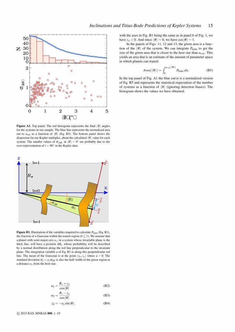
Figure A1. Top panel: The red histogram represents the final 〈θ〉 anglesfor the systems in our sample. The blue line represents the normalised areaout to acrit as a function of 〈θ〉 (Eq. B5). The bottom panel shows thedispersion for our Kepler multiples, about the calculated 〈θ〉 value for eachsystem. The smaller values of σ〈∆θ〉 at 〈θ〉 ∼ 0◦ are probably due to theover-representation of i = 90◦ in the Kepler data.

(x0,z0)

b=1

b=1

b=0

u1

u2

σ∆θ

R*

z

x

a j

σ j

⟨θ⟩

u=0

u=1

Figure B1. Illustration of the variables required to calculate Ptrans (Eq. B1),the fraction of a Gaussian within the transit region (b . 1). We assume thata planet with semi-major axis a j , in a system whose invariable plane is thethick line, will have a position ∆θ j , whose probability will be describedby a normal distribution along the red line perpendicular to the invariantplane. The integration variable u of Eq. B1 is along this perpendicular redline. The mean of the Gaussian is at the point (xo,zo) where u = 0. Thestandard deviation σ j = a jσ∆θ is also the half-width of the green region ata distance a j from the host star.

u1 =R∗+ zo

cos〈θ〉(B2)

u2 =R∗− zo

cos〈θ〉(B3)

z0 =−a j sin〈θ〉. (B4)

with the axes in Fig. B1 being the same as in panel b of Fig. 1, wehave zo < 0. And since 〈θ〉 ∼ 0, we have cos〈θ〉 ∼ 1.

In the panels of Figs. 11, 12 and 13, the green area is a func-tion of the 〈θ〉 of the system. We can integrate Ptrans to get thesize of the green area that is closer to the host star than acrit . Thisyields an area that is an estimate of the amount of parameter spacein which planets can transit:

Area(〈θ〉) =∫ acrit (〈θ〉)

0Ptrans da. (B5)

In the top panel of Fig. A1 the blue curve is a normalized versionof Eq. B5 and represents the statistical expectation of the numberof systems as a function of 〈θ〉 (ignoring detection biases). Thehistogram shows the values we have obtained.

c© 2015 RAS, MNRAS 000, 1–19

16 T. Bovaird, C. H. Lineweaver and S. K. Jacobsen

APPENDIX C: TABLES OF PLANET PREDICTIONS

Table C1: 77 Planet predictions with a high geometric probability to transit (Ptrans > 0.55) in 40 Kepler systems

System Number γ ∆γa(

χ2

d.o.f.

)i

(χ2

d.o.f.

)f

Inserted Period a Rmaxb Teff Ptrans

Inserted Planet # (days) (AU) (R⊕) (K)KOI-1198 2 2.2 0.3 7.19 0.74 1 2.1±0.4 0.03 1.3 1642 1.00

2 4.3±0.7 0.06 1.5 1297 1.00KOI-1955 4 3.4 0.2 10.23 0.19 1 2.6±0.3 0.04 0.9 1568 1.00

2 4.1±0.5 0.05 1.0 1347 1.003 6.4±0.7 0.07 1.2 1157 0.994 10.1±1.1 0.10 1.3 994 0.94

KOI-1082 2 23.0 5.0 5.02 0.06 1 1.8±0.2 0.03 1.0 1184 1.002 2.8±0.3 0.04 1.1 1029 1.003 E c 14.7±1.4 0.11 1.6 588 0.72

KOI-952 1 2.2 5.2 2.36 0.76 1 1.5±0.3 0.02 0.9 904 1.00KOI-500 2 7.6 1.9 5.47 0.18 1 1.5±0.2 0.02 1.2 1091 1.00

2 2.1±0.2 0.03 1.3 960 1.00KOI-4032 2 0.9 1.9 1.20 0.27 1 3.4±0.2 0.04 0.8 1347 1.00

2 4.5±0.2 0.05 0.9 1224 0.993 E 6.9±0.3 0.07 1.0 1061 0.91

KOI-707 1 3.2 2.2 3.69 0.90 1 8.9±0.8 0.09 2.0 1162 1.00KOI-1336 2 1.3 65.6 1.07 0.19 1 6.7±0.7 0.07 1.7 1053 0.98

2 25.1±2.5 0.17 2.4 679 0.64KOI-2859 1 10.2 -1.0 1.69 0.16 1 2.4±0.1 0.03 0.6 1242 0.98KOI-250 5 0.7 1.1 2.26 0.14 1 4.8±0.4 0.05 1.2 686 0.96

2 6.6±0.6 0.06 1.3 616 0.913 9.2±0.8 0.07 1.4 553 0.83

KOI-168 0 - - 0.14 - 1 E 22.6±1.2 0.17 2.6 909 0.952 E 33.2±1.4 0.21 2.9 800 0.873 E 48.6±1.7 0.28 3.2 704 0.764 E 71.3±2.2 0.36 3.5 620 0.64

KOI-2585 0 - - 0.55 - 1 E 14.8±0.7 0.12 1.1 967 0.952 E 20.7±0.8 0.15 1.2 865 0.873 E 28.9±0.9 0.19 1.3 774 0.784 E 40.4±1.1 0.24 1.4 692 0.675 E 56.4±1.3 0.30 1.6 619 0.57

KOI-1052 2 115.4 40.4 1.36 0.01 1 10.8±1.2 0.10 1.6 909 0.942 27.1±2.8 0.18 2.0 669 0.69

KOI-505 3 1.6 0.1 8.20 0.56 1 21.9±2.5 0.15 4.5 788 0.922 34.7±3.9 0.20 5.1 676 0.783 55±7 0.27 5.7 580 0.62

KOI-1831 1 1.3 0.2 2.54 1.11 1 8.2±1.1 0.08 0.9 739 0.91KOI-248 1 18.3 80.8 2.48 0.13 1 4.2±0.5 0.04 1.4 633 0.89KOI-880 1 4.0 22.4 1.35 0.28 1 11.8±2.0 0.10 2.1 761 0.89KOI-1567 2 5.9 44.8 1.51 0.07 1 11.4±1.2 0.10 2.0 668 0.89

2 28.0±2.9 0.18 2.5 494 0.62KOI-1952 2 85.6 16.6 3.26 0.01 1 12.1±1.2 0.10 1.5 828 0.87

2 18.3±1.8 0.14 1.6 720 0.75KOI-351 4 0.5 1.0 5.78 0.65 1 15.4±1.7 0.13 1.4 813 0.87

2 23.9±2.5 0.17 1.6 702 0.743 37.1±3.9 0.23 1.8 607 0.60

KOI-701 6 18.0 7.4 4.04 0.01 1 8.4±0.8 0.07 0.6 621 0.87KOI-1306 1 5.7 0.4 4.12 0.62 1 13.7±2.1 0.11 1.5 756 0.85KOI-2722 0 - - 0.54 - 1 E 23.4±1.5 0.17 1.4 774 0.78

2 E 33.0±1.8 0.21 1.5 690 0.673 E 46.5±2.3 0.27 1.6 615 0.56

KOI-1358 0 - - 0.01 - 1 E 13.6±1.0 0.10 1.6 522 0.742 E 21.0±1.3 0.14 1.8 451 0.60

KOI-1627 0 - - 0.24 - 1 E 16.6±1.2 0.13 1.9 586 0.732 E 27.4±1.5 0.17 2.1 497 0.57

KOI-1833 0 - - 0.74 - 1 E 11.3±0.6 0.08 2.0 514 0.722 E 16.4±0.7 0.10 2.2 455 0.60

KOI-3158 0 - - 0.23 - 1 E 12.7±0.6 0.09 0.4 566 0.712 E 16.4±0.7 0.11 0.4 520 0.62

KOI-2055 0 - - 0.29 - 1 E 13.6±1.0 0.11 1.3 703 0.702 E 20.6±1.2 0.14 1.5 612 0.56

KOI-245 3 1.0 1.3 1.56 0.17 1 16.8±0.9 0.12 0.3 582 0.702 26.1±1.4 0.16 0.3 502 0.56

KOI-749 0 - - 0.49 - 1 E 11.4±0.6 0.10 1.5 711 0.692 E 16.4±0.7 0.12 1.7 630 0.57

KOI-730 0 - - 0.33 - 1 E 27.9±1.5 0.18 2.3 620 0.692 E 39.0±1.8 0.22 2.5 554 0.58

KOI-719 1 1.1 1.5 1.36 0.66 1 14.8±2.0 0.11 0.8 514 0.69KOI-1060 0 - - 0.22 - 1 E 32.7±2.6 0.22 2.1 703 0.68KOI-3083 0 - - 0.56 - 1 E 13.2±0.5 0.11 0.7 751 0.66

2 E 16.9±0.5 0.13 0.7 692 0.57KOI-156 0 - - 0.10 - 1 E 17.9±1.0 0.12 1.6 476 0.61KOI-137 0 - - 0.13 - 1 E 31.2±3.1 0.19 3.1 539 0.60KOI-1151 0 - - 0.85 - 1 E 33.0±2.2 0.20 1.0 564 0.59KOI-1015 0 - - 0.62 - 1 E 36.1±3.5 0.22 2.3 590 0.58KOI-2029 0 - - 0.31 - 1 E 23.7±1.6 0.15 0.9 514 0.56KOI-664 0 - - 0.06 - 1 E 40.3±3.0 0.23 1.5 618 0.56

a ∆γ = (γ1− γ2)/γ2 where γ1 and γ2 are the highest and second highest γ values for that system respectively (see Bovaird & Lineweaver (2013)).b Rmax is calculated by applying the lowest SNR of the detected planets in the system to the period of the inserted planet. See Eq. 7.c A planet number followed by “E" indicates the planet is extrapolated (has a larger period than the outermost detected planet in the system).

c© 2015 RAS, MNRAS 000, 1–19

Inclinations and Titius-Bode Predictions of Kepler Systems 17

Table C2: All 228 Planet Predictions in 151 Systems (Table C1 is a high Ptrans subset of this table)

System Number γ ∆γa(

χ2

d.o.f.

)i

(χ2

d.o.f.

)f

Inserted Period a Rmaxb Teff

e Ptransd

Inserted Planet # (days) (AU) (R⊕) (K)KOI-1198 2 2.2 0.3 7.19 0.74 1 2.1±0.4 0.03 1.3 1642 1.00

2 4.3±0.7 0.06 1.5 1297 1.003 E c 73±12 0.37 3.1 505 0.41

KOI-1955 4 3.4 0.2 10.23 0.19 1 2.6±0.3 0.04 0.9 1568 1.002 4.1±0.5 0.05 1.0 1347 1.003 6.4±0.7 0.07 1.2 1157 0.994 10.1±1.1 0.10 1.3 994 0.945 E 62±7 0.33 2.0 541 0.42

KOI-1082 2 23.0 5.0 5.02 0.06 1 1.8±0.2 0.03 1.0 1184 1.002 2.8±0.3 0.04 1.1 1029 1.003 E 14.7±1.4 0.11 1.6 588 0.72

KOI-952 1 2.2 5.2 2.36 0.76 1 1.5±0.3 0.02 0.9 904 1.002 E 40.0±6.2 0.19 2.1 299 0.36

KOI-500 2 7.6 1.9 5.47 0.18 1 1.5±0.2 0.02 1.2 1091 1.002 2.1±0.2 0.03 1.3 960 1.003 E 14.5±1.3 0.10 2.2 506 0.50

KOI-4032 2 0.9 1.9 1.20 0.27 1 3.4±0.2 0.04 0.8 1347 1.002 4.5±0.2 0.05 0.9 1224 0.993 E 6.9±0.3 0.07 1.0 1061 0.91

KOI-707 1 3.2 2.2 3.69 0.90 1 8.9±0.8 0.09 2.0 1162 1.002 E 68±7 0.35 3.3 590 0.50

KOI-1336 2 1.3 65.6 1.07 0.19 1 6.7±0.7 0.07 1.7 1053 0.982 25.1±2.5 0.17 2.4 679 0.643 E 60±6 0.31 3.0 507 0.39

KOI-2859 1 10.2 -1.0 1.69 0.16 1 2.4±0.1 0.03 0.6 1242 0.982 E 5.1±0.3 0.05 0.8 967 0.54

KOI-250 5 0.7 1.1 2.26 0.14 1 4.8±0.4 0.05 1.2 686 0.962 6.6±0.6 0.06 1.3 616 0.913 9.2±0.8 0.07 1.4 553 0.834 24.1±1.9 0.14 1.8 401 0.535 33.2±2.6 0.17 2.0 360 0.446 E 63.3±5.0 0.27 2.3 290 0.29

KOI-168 0 - - 0.14 - 1 E 22.6±1.2 0.17 2.6 909 0.952 E 33.2±1.4 0.21 2.9 800 0.873 E 48.6±1.7 0.28 3.2 704 0.764 E 71.3±2.2 0.36 3.5 620 0.645 E 104.5±2.7 0.46 3.8 546 0.52

KOI-2585 0 - - 0.55 - 1 E 14.8±0.7 0.12 1.1 967 0.952 E 20.7±0.8 0.15 1.2 865 0.873 E 28.9±0.9 0.19 1.3 774 0.784 E 40.4±1.1 0.24 1.4 692 0.675 E 56.4±1.3 0.30 1.6 619 0.57

KOI-1052 2 115.4 40.4 1.36 0.01 1 10.8±1.2 0.10 1.6 909 0.942 27.1±2.8 0.18 2.0 669 0.693 E 110±20 0.46 2.8 423 0.31

KOI-505 3 1.6 0.1 8.20 0.56 1 21.9±2.5 0.15 4.5 788 0.922 34.7±3.9 0.20 5.1 676 0.783 55±7 0.27 5.7 580 0.624 E 140±20 0.51 7.2 426 0.36

KOI-1831 1 1.3 0.2 2.54 1.11 1 8.2±1.1 0.08 0.9 739 0.912 E 100±20 0.41 1.7 316 0.25

KOI-248 1 18.3 80.8 2.48 0.13 1 4.2±0.5 0.04 1.4 633 0.892 E 30.1±3.3 0.16 2.2 329 0.30

KOI-880 1 4.0 22.4 1.35 0.28 1 11.8±2.0 0.10 2.1 761 0.892 E 120±20 0.45 3.7 354 0.27

KOI-1567 2 5.9 44.8 1.51 0.07 1 11.4±1.2 0.10 2.0 668 0.892 28.0±2.9 0.18 2.5 494 0.623 E 69±8 0.32 3.1 366 0.37

KOI-1952 2 85.6 16.6 3.26 0.01 1 12.1±1.2 0.10 1.5 828 0.872 18.3±1.8 0.14 1.6 720 0.753 E 64±7 0.31 2.2 474 0.38

KOI-351 4 0.5 1.0 5.78 0.65 1 15.4±1.7 0.13 1.4 813 0.872 23.9±2.5 0.17 1.6 702 0.743 37.1±3.9 0.23 1.8 607 0.604 140±20 0.54 2.4 391 0.275 E 520±60 1.31 3.4 252 0.12

KOI-701 6 18.0 7.4 4.04 0.01 1 8.4±0.8 0.07 0.6 621 0.872 26.6±2.6 0.15 0.8 423 0.523 39.1±3.7 0.19 0.9 372 0.414 57±6 0.25 1.0 327 0.335 84±8 0.32 1.1 288 0.256 180±20 0.54 1.3 223 0.157 E 390±40 0.90 1.6 172 0.09

KOI-1306 1 5.7 0.4 4.12 0.62 1 13.7±2.1 0.11 1.5 756 0.852 E 55±9 0.28 2.1 476 0.43

KOI-2722 0 - - 0.54 - 1 E 23.4±1.5 0.17 1.4 774 0.782 E 33.0±1.8 0.21 1.5 690 0.673 E 46.5±2.3 0.27 1.6 615 0.56

KOI-1358 0 - - 0.01 - 1 E 13.6±1.0 0.10 1.6 522 0.742 E 21.0±1.3 0.14 1.8 451 0.60

KOI-1627 0 - - 0.24 - 1 E 16.6±1.2 0.13 1.9 586 0.732 E 27.4±1.5 0.17 2.1 497 0.57

KOI-1833 0 - - 0.74 - 1 E 11.3±0.6 0.08 2.0 514 0.722 E 16.4±0.7 0.10 2.2 455 0.60

KOI-3158 0 - - 0.23 - 1 E 12.7±0.6 0.09 0.4 566 0.712 E 16.4±0.7 0.11 0.4 520 0.62

continued

c© 2015 RAS, MNRAS 000, 1–19

18 T. Bovaird, C. H. Lineweaver and S. K. Jacobsen

Table C2: All 228 Planet Predictions in 151 Systems (Table C1 is a high Ptrans subset of this table)

System Number γ ∆γa(

χ2

d.o.f.

)i

(χ2

d.o.f.

)f

Inserted Period a Rmaxb Teff

e Ptransd

Inserted Planet # (days) (AU) (R⊕) (K)3 E 21.1±0.8 0.13 0.5 478 0.55

KOI-2055 0 - - 0.29 - 1 E 13.6±1.0 0.11 1.3 703 0.702 E 20.6±1.2 0.14 1.5 612 0.56

KOI-245 3 1.0 1.3 1.56 0.17 1 16.8±0.9 0.12 0.3 582 0.702 26.1±1.4 0.16 0.3 502 0.563 32.6±1.7 0.18 0.3 467 0.504 E 63.1±3.3 0.28 0.4 374 0.33

KOI-749 0 - - 0.49 - 1 E 11.4±0.6 0.10 1.5 711 0.692 E 16.4±0.7 0.12 1.7 630 0.57

KOI-730 0 - - 0.33 - 1 E 27.9±1.5 0.18 2.3 620 0.692 E 39.0±1.8 0.22 2.5 554 0.58

KOI-719 1 1.1 1.5 1.36 0.66 1 14.8±2.0 0.11 0.8 514 0.692 E 88±12 0.35 1.2 284 0.24

KOI-1060 0 - - 0.22 - 1 E 32.7±2.6 0.22 2.1 703 0.682 E 52.7±3.5 0.30 2.3 599 0.53

KOI-3083 0 - - 0.56 - 1 E 13.2±0.5 0.11 0.7 751 0.662 E 16.9±0.5 0.13 0.7 692 0.57

KOI-156 0 - - 0.10 - 1 E 17.9±1.0 0.12 1.6 476 0.61KOI-137 0 - - 0.13 - 1 E 31.2±3.1 0.19 3.1 539 0.60KOI-1151 0 - - 0.85 - 1 E 33.0±2.2 0.20 1.0 564 0.59KOI-1015 0 - - 0.62 - 1 E 36.1±3.5 0.22 2.3 590 0.58KOI-2029 0 - - 0.31 - 1 E 23.7±1.6 0.15 0.9 514 0.56KOI-664 0 - - 0.06 - 1 E 40.3±3.0 0.23 1.5 618 0.56KOI-2693 0 - - 0.01 - 1 E 19.1±1.4 0.12 1.0 430 0.53KOI-1590 0 - - 0.64 - 1 E 28.7±3.3 0.16 1.8 452 0.53KOI-279 0 - - 0.13 - 1 E 56±6 0.30 1.3 586 0.53KOI-1930 0 - - 0.60 - 1 E 72±7 0.35 2.3 541 0.52KOI-70 1 7.4 2.9 3.51 0.42 1 39.1±5.4 0.22 1.2 498 0.52

2 E 130±20 0.49 1.7 331 0.24KOI-720 0 - - 0.14 - 1 E 34.8±3.6 0.20 2.9 477 0.51KOI-1860 0 - - 0.02 - 1 E 49.5±5.6 0.27 1.7 512 0.49KOI-1475 0 - - 0.94 - 1 E 24.6±3.0 0.14 1.7 377 0.48KOI-1194 0 - - 0.52 - 1 E 29.0±2.5 0.16 1.8 374 0.47KOI-2025 0 - - 0.21 - 1 E 40.5±2.4 0.24 2.3 647 0.47KOI-733 0 - - 0.22 - 1 E 35.5±3.5 0.20 2.8 437 0.46KOI-2169 0 - - 0.87 - 1 E 7.6±0.4 0.07 0.7 868 0.46KOI-2163 0 - - 0.06 - 1 E 46.3±3.1 0.26 1.7 532 0.44KOI-3319 0 - - 0.01 - 1 E 45.9±5.3 0.25 2.1 517 0.44KOI-2352 0 - - 0.28 - 1 E 20.3±1.2 0.16 1.1 845 0.44KOI-1681 0 - - 0.15 - 1 E 12.7±1.1 0.09 1.3 415 0.44KOI-1413 0 - - 0.14 - 1 E 56.2±3.8 0.28 1.8 458 0.44KOI-2597 0 - - 0.13 - 1 E 17.7±1.0 0.14 1.8 791 0.43KOI-2220 0 - - 0.19 - 1 E 19.1±1.6 0.14 1.2 695 0.42KOI-1161 0 - - 0.18 - 1 E 21.4±1.9 0.14 2.1 574 0.42KOI-582 0 - - 0.08 - 1 E 30.3±2.3 0.18 1.8 466 0.41KOI-82 0 - - 0.92 - 1 E 38.3±2.9 0.21 0.9 408 0.41KOI-157 1 3.7 6.9 3.15 0.69 1 75±8 0.34 2.7 439 0.41

2 E 170±20 0.60 3.4 334 0.24KOI-864 0 - - 0.09 - 1 E 44.0±4.6 0.24 2.9 453 0.40KOI-939 0 - - 0.24 - 1 E 20.3±2.1 0.15 1.9 640 0.40KOI-898 0 - - 0.08 - 1 E 39.1±3.6 0.20 2.8 360 0.40KOI-841 2 7.1 0.4 4.35 0.15 1 63±11 0.31 2.7 409 0.39

2 130±30 0.51 3.3 320 0.253 E 580±100 1.35 4.7 196 0.09

KOI-408 0 - - 0.51 - 1 E 59±7 0.29 2.6 461 0.39KOI-1909 0 - - 0.26 - 1 E 55±6 0.29 1.9 500 0.38KOI-2715 0 - - 0.62 - 1 E 26.1±2.9 0.14 3.9 379 0.38KOI-1278 0 - - 0.52 - 1 E 73±7 0.35 2.0 455 0.38KOI-1867 0 - - 0.53 - 1 E 31.3±3.6 0.16 1.7 323 0.37KOI-899 0 - - 0.01 - 1 E 33.1±3.5 0.16 1.9 293 0.37KOI-1589 0 - - 0.56 - 1 E 82±9 0.37 2.4 440 0.37KOI-884 0 - - 0.45 - 1 E 53±7 0.25 2.9 362 0.37KOI-829 0 - - 0.07 - 1 E 76±8 0.36 3.5 442 0.37KOI-94 0 - - 0.19 - 1 E 130±20 0.55 4.2 452 0.36KOI-2038 0 - - 0.11 - 1 E 37.0±2.3 0.21 1.8 494 0.36KOI-1557 0 - - 0.58 - 1 E 18.2±1.9 0.12 2.0 499 0.35KOI-571 2 19.9 5.2 4.87 0.07 1 40.9±5.6 0.19 0.8 294 0.35

2 73±10 0.28 0.9 242 0.243 E 230±40 0.61 1.2 164 0.11

KOI-1905 0 - - 0.01 - 1 E 72±8 0.32 1.7 374 0.34KOI-116 0 - - 0.34 - 1 E 86±10 0.38 1.3 425 0.34KOI-2732 0 - - 0.22 - 1 E 100±20 0.44 1.3 426 0.34KOI-665 0 - - 0.01 - 1 E 11.2±1.0 0.10 1.5 893 0.34KOI-1931 0 - - 0.20 - 1 E 15.2±0.8 0.12 1.5 661 0.33KOI-886 0 - - 0.46 - 1 E 33.2±2.2 0.16 1.6 298 0.32KOI-1432 0 - - 0.07 - 1 E 87±13 0.38 2.0 397 0.32KOI-945 0 - - 0.04 - 1 E 107±7 0.46 2.6 424 0.32KOI-869 0 - - 0.08 - 1 E 84±12 0.35 3.8 349 0.31KOI-111 0 - - 0.03 - 1 E 110±20 0.42 2.8 376 0.30KOI-1364 0 - - 0.41 - 1 E 34.9±3.3 0.20 3.0 508 0.30KOI-1832 0 - - 0.03 - 1 E 110±20 0.44 3.6 381 0.30KOI-658 0 - - 0.60 - 1 E 20.7±1.8 0.15 1.4 649 0.30KOI-1895 0 - - 0.11 - 1 E 64±6 0.27 2.6 289 0.30KOI-2926 0 - - 0.49 - 1 E 73±8 0.27 2.8 260 0.29KOI-1647 0 - - 0.07 - 1 E 74±9 0.34 2.0 460 0.29KOI-941 0 - - 0.36 - 1 E 75±12 0.32 4.7 343 0.29

continued

c© 2015 RAS, MNRAS 000, 1–19

Inclinations and Titius-Bode Predictions of Kepler Systems 19

Table C2: All 228 Planet Predictions in 151 Systems (Table C1 is a high Ptrans subset of this table)

System Number γ ∆γa(

χ2

d.o.f.

)i

(χ2

d.o.f.

)f

Inserted Period a Rmaxb Teff

e Ptransd

Inserted Planet # (days) (AU) (R⊕) (K)KOI-3741 0 - - 0.01 - 1 E 35.3±3.1 0.21 2.2 709 0.28KOI-700 0 - - 0.91 - 1 E 120±20 0.48 2.1 388 0.28KOI-1563 0 - - 0.62 - 1 E 26.9±2.5 0.17 3.6 491 0.28KOI-2135 0 - - 0.12 - 1 E 140±20 0.53 1.9 414 0.28KOI-2433 0 - - 0.55 - 1 E 150±20 0.57 2.9 395 0.28KOI-2086 0 - - 0.33 - 1 E 15.2±0.6 0.13 2.7 933 0.27KOI-1102 0 - - 0.75 - 1 E 32.4±2.7 0.20 2.8 630 0.27KOI-3097 0 - - 0.31 - 1 E 15.6±0.6 0.13 1.3 1033 0.27KOI-1445 0 - - 0.01 - 1 E 150±30 0.59 1.4 391 0.27KOI-232 0 - - 0.93 - 1 E 110±20 0.46 2.1 391 0.26KOI-520 0 - - 0.18 - 1 E 110±20 0.42 1.8 314 0.26KOI-2707 0 - - 0.29 - 1 E 110±20 0.45 2.3 335 0.25KOI-152 0 - - 0.64 - 1 E 160±20 0.60 3.6 381 0.25KOI-1332 0 - - 0.03 - 1 E 170±30 0.63 3.8 337 0.25KOI-2485 0 - - 0.17 - 1 E 16.4±1.2 0.12 1.8 575 0.25KOI-877 0 - - 0.32 - 1 E 40.0±3.4 0.20 1.6 343 0.24KOI-775 0 - - 0.04 - 1 E 78±9 0.30 2.4 253 0.24KOI-757 0 - - 0.01 - 1 E 110±20 0.41 4.2 295 0.24KOI-510 0 - - 0.05 - 1 E 78±11 0.34 3.5 413 0.24KOI-117 0 - - 0.42 - 1 E 23.3±2.0 0.17 1.4 692 0.23KOI-935 0 - - 0.03 - 1 E 180±30 0.68 4.1 374 0.23KOI-285 0 - - 0.04 - 1 E 94±9 0.43 2.2 490 0.22KOI-671 0 - - 0.62 - 1 E 26.4±2.0 0.17 1.5 614 0.22KOI-834 0 - - 0.84 - 1 E 120±20 0.47 2.5 351 0.22KOI-509 0 - - 0.22 - 1 E 120±20 0.46 2.5 334 0.22KOI-904 0 - - 0.93 - 1 E 100±20 0.37 2.2 252 0.22KOI-723 0 - - 0.04 - 1 E 74±10 0.33 4.2 357 0.22KOI-1436 0 - - 0.19 - 1 E 31.3±3.6 0.19 2.3 555 0.21KOI-435 2 1.8 0.3 6.69 0.84 1 160±30 0.55 2.3 321 0.21

2 320±60 0.90 2.8 252 0.133 E 1380±250 2.35 4.0 155 0.05

KOI-2073 0 - - 0.08 - 1 E 130±20 0.46 2.8 274 0.20KOI-812 0 - - 0.04 - 1 E 110±20 0.38 2.5 224 0.20KOI-474 0 - - 0.54 - 1 E 230±40 0.77 3.8 336 0.20KOI-907 0 - - 0.91 - 1 E 250±50 0.76 4.5 309 0.19KOI-1422 0 - - 0.04 - 1 E 110±20 0.37 1.9 198 0.19KOI-710 0 - - 0.69 - 1 E 12.5±0.7 0.12 1.7 998 0.19KOI-623 0 - - 0.40 - 1 E 42.2±3.5 0.23 1.3 592 0.19KOI-282 0 - - 0.01 - 1 E 280±50 0.83 1.5 299 0.19KOI-620 0 - - 0.84 - 1 E 230±20 0.74 7.6 298 0.18KOI-3925 0 - - 0.38 - 1 E 17.9±1.6 0.13 3.5 779 0.18KOI-2167 0 - - 0.05 - 1 E 260±50 0.82 1.8 303 0.17KOI-1426 0 - - 0.02 - 1 E 290±30 0.88 5.3 294 0.16KOI-1127 0 - - 0.81 - 1 E 14.2±1.1 0.12 2.0 681 0.16KOI-191 0 - - 0.99 - 1 E 180±40 0.61 3.4 301 0.16KOI-1430 0 - - 0.98 - 1 E 200±30 0.57 3.2 215 0.15KOI-806 0 - - 0.16 - 1 E 310±40 0.89 2.5 247 0.15KOI-612 0 - - 0.10 - 1 E 290±40 0.79 3.6 235 0.15KOI-481 0 - - 0.02 - 1 E 160±40 0.56 4.0 282 0.14KOI-2714 0 - - 0.09 - 1 E 640±120 1.55 3.4 272 0.13KOI-1258 0 - - 0.96 - 1 E 430±70 1.11 5.1 218 0.10KOI-564 0 - - 0.77 - 1 E 530±110 1.28 4.3 222 0.10KOI-1922 0 - - 0.02 - 1 E 790±220 1.69 2.9 199 0.08KOI-2183 0 - - 0.70 - 1 E 770±190 1.64 3.0 188 0.07KOI-518 0 - - 0.84 - 1 E 940±190 1.59 3.1 124 0.05KOI-2842 0 - - 0.27 - 1 E 9.5±0.8 0.07 3.2 559 0.00

a ∆γ = (γ1− γ2)/γ2 where γ1 and γ2 are the highest and second highest γ values for that system respectively (see BL13).b Rmax is calculated by applying the lowest SNR of the detected planets in the system to the period of the inserted planet. See Eq. 7.c A planet number followed by “E" indicates the planet is extrapolated (has a larger period than the outermost detected planet in the system).d Ptrans values > 0.55 are shown in bold, indicating a higher probability to transit.e Teff values between Mars and Venus (206 K to 300 K, assuming an albedo of 0.3) are shown in bold.

c© 2015 RAS, MNRAS 000, 1–19