using smoothing techniques to improve the performance of
TRANSCRIPT

UNLV Theses, Dissertations, Professional Papers, and Capstones
5-2011
Using smoothing techniques to improve the performance of Using smoothing techniques to improve the performance of
Hidden Markov’s Model Hidden Markov’s Model
Sweatha Boodidhi University of Nevada, Las Vegas
Follow this and additional works at: https://digitalscholarship.unlv.edu/thesesdissertations
Part of the Theory and Algorithms Commons
Repository Citation Repository Citation Boodidhi, Sweatha, "Using smoothing techniques to improve the performance of Hidden Markov’s Model" (2011). UNLV Theses, Dissertations, Professional Papers, and Capstones. 1007. http://dx.doi.org/10.34917/2349611
This Thesis is protected by copyright and/or related rights. It has been brought to you by Digital Scholarship@UNLV with permission from the rights-holder(s). You are free to use this Thesis in any way that is permitted by the copyright and related rights legislation that applies to your use. For other uses you need to obtain permission from the rights-holder(s) directly, unless additional rights are indicated by a Creative Commons license in the record and/or on the work itself. This Thesis has been accepted for inclusion in UNLV Theses, Dissertations, Professional Papers, and Capstones by an authorized administrator of Digital Scholarship@UNLV. For more information, please contact [email protected].
USING SMOOTHING TECHNIQUES TO IMPROVE THE PERFORMANCE
OF HIDDEN MARKOV’S MODEL
by
Sweatha Boodidhi
Bachelor of Technology
Jawaharlal Nehru Technological University, India May 2007
A thesis submitted in partial fulfillment of the requirements for the
Master of Science in Computer Science School of Computer Science
Howard R. Hughes College of Engineering
Graduate College University of Nevada, Las Vegas
May 2011

Copyright by Sweatha Boodidhi 2011 All Rights Reserved

ii
THE GRADUATE COLLEGE We recommend the thesis prepared under our supervision by Sweatha Boodidhi entitled Using Smoothing Techniques to Improve the Performance of Hidden Markov’s Model be accepted in partial fulfillment of the requirements for the degree of Master of Science in Computer Science School of Computer Science Kazem Taghva, Committee Chair Ajoy K. Datta, Committee Member Laxmi P Gewali, Committee Member Venkatesan Muthukumar, Graduate Faculty Representative Ronald Smith, Ph. D., Vice President for Research and Graduate Studies and Dean of the Graduate College May 2011

iii
ABSTRACT
Using Smoothing Techniques to Improve the Performance of Hidden Markov’s Models
by
Sweatha Boodidhi
Dr. Kazem Taghva, Examination committee Chair Professor of Computer Science University Of Nevada Las Vegas
The result of training a HMM using supervised training is estimated
probabilities for emissions and transitions. There are two difficulties with
this approach Firstly, sparse training data causes poor probability
estimates. Secondly, unseen probabilities have emission probability of
zero. In this thesis, we report on different smoothing techniques and
their implementations. We further report on our experimental results
using standard precision and recall for various smoothing techniques.

iv
ACKNOWLEDGEMENTS
I would like to thank my advisor, Dr. Kazem Taghva , for all his help and
support in my pursuit of a Master’s degree. Throughout this process he
has provided support and encouragement in my thesis and my studies.
His advice and enthusiasm were critical to the success of this effort. I
would also like to thank Dr. Ajoy K Datta for serving on my advisory
Committee, as well as Graduate coordinator and for his time in reviewing
the prospectus and his help, advice and guidance during my course
work.
I would also like to thank Dr. Laxmi P. Gewali and Dr. Venkatesan
Muthukumar for their time in reviewing the prospectus, participation in
defense, and counseling of the thesis as the committee members.
I would also like to thank my husband Venkat Mudupu whose
suggestions and advices have been great help for me.
I would also like to express my heartiest gratitude to my parents
for their unconditional support, love, and affection. A special thanks to
my friends for their unrelenting support and motivation throughout this
research activity.
Finally, I would like to thank Mario Martin and Sharron, staff of
the Computer Science Engineering department, for providing me with all
resources for my defense.

v
TABLE OF CONTENTS
ABSTRACT ........................................................................................... iii
ACKNOWLEDGEMENTS ....................................................................... iv
TABLE OF CONTENTS ........................................................................... v
LIST OF FIGURES ................................................................................vii
CHAPTER 1 INTRODUCTION ................................................................. 1
1.1 Thesis Overview ............................................................................ 3
CHAPTER 2 HIDDEN MARKOV MODEL ................................................. 4
2.1 Definition of HMM ........................................................................ 4
2.1.1 Examples on HMM .............................................................. 5
2.2 Main Issues Using HMM ............................................................... 6
2.2.1 Evaluation Problem ................................................................ 7
2.2.1.1 Forward recursion for HMM .............................................. 8
2.2.1.2 Backward recursion for HMM ........................................... 9
2.2.2 Decoding Problem ................................................................. 10
2.2.2.1 Viterbi algorithm ............................................................ 10
2.2.3 Learning Problem ................................................................. 12
2.2.3.1 Maximum Likelihood Estimation .................................... 13
CHAPTER 3 SMOOTHING .................................................................... 14
3.1 What is Smoothing ..................................................................... 14
3.2 Why Smoothing is used in HMM? ............................................... 14
3.2.1 Where we use Smoothing in HMM? ....................................... 14
3.2.2 Maximum Likelihood Estimation ........................................... 15
3.3 How Smoothing works in HMM ................................................... 16
3.3.1 Examples.............................................................................. 16
3.3.1.1 Example 1 ...................................................................... 16
3.3.1.2 Example 2 ...................................................................... 16
3.3.1.3 Example 3 ...................................................................... 17
3.4 Smoothing Techniques ............................................................... 17
3.4.1 Absolute Discounting ............................................................ 17
3.4.2 Laplace Smoothing ............................................................... 18
3.4.3 Good-Turing Estimation ....................................................... 18
3.4.4 Shrinkage ............................................................................. 19
CHAPTER 4 IMPLEMENTATION ........................................................... 21
4.1 Supervised Learning ................................................................... 21
4.1.1 Maximum Likelihood Estimation (MLE) ................................. 21
4.2 Laplace Smoothing ..................................................................... 23
4.3 Absolute Discounting.................................................................. 25
vi
CHAPTER 5 RESULTS ......................................................................... 29
5.1 Using HMM Model ...................................................................... 29
5.1.1 HMM Model How it Looks ..................................................... 29
5.1.2 Results on HMM and How it Works ....................................... 30
5.2 Comparison of Two Smoothing Techniques ................................. 32
5.2.1 Equation on MLE .................................................................. 32
5.2.2 Equation on Laplace Smoothing ............................................ 32
5.2.3 Equation on Absolute Discounting ........................................ 32
5.3 Results on Laplace Smoothing .................................................... 33
5.4 Results on Absolute Discounting ................................................ 34
5.5 Precision is defined as ................................................................ 36
5.6 Recall is defined as ..................................................................... 36
5.7 Harmonic Mean .......................................................................... 36
5.8 Results on Evaluation ................................................................. 36
5.8.1 Without Using Smoothing Techniques................................... 36
5.8.2 Using Smoothing Techniques ................................................ 37
5.8.2.1 Laplace Smoothing ......................................................... 37
5.8.2.2 Absolute Discounting ..................................................... 37
CHAPTER 6 CONCLUSIONS AND FUTURE WORK ............................... 38
BIBLIOGRAPHY ................................................................................... 39
VITA .................................................................................................... 40

vii
LIST OF FIGURES
Figure 1 Example on Hidden Markov’s Model ......................................... 5
Figure 2 Trellis Representation of HMM ................................................. 7
Figure 3 Forward Recursion of HMM ...................................................... 8
Figure 4 Backward Recursion of HMM ................................................... 9
Figure 5 Viterbi Algorithm.................................................................... 11
Figure 6 Algorithm Counting for in MLE .............................................. 23
Figure 7 Screen shot on Laplace smoothing ......................................... 24
Figure 8 Screen Shot on Absolute Discounting ..................................... 25
Figure 9 Screen Shot on Absolute Discounting ..................................... 26
Figure 10 Screen Shot on Absolute Discounting ................................... 26
Figure 11 Screen Shot on Absolute Discounting ................................... 27
Figure 12 Screen Shot on Absolute Discounting ................................... 27
Figure 13 Screen Shot on Absolute Discounting ................................... 28
Figure 14 HMM Model ......................................................................... 29
Figure 15 HMM Model Data ................................................................. 30
Figure 16 HMM Train Data .................................................................. 31
Figure 17 Laplace Smoothing Result .................................................... 33
Figure 18 Laplace Smoothing Result .................................................... 34
Figure 19 Laplace Smoothing Result .................................................... 34
Figure 20 Absolute Discounting Result ................................................ 35

1
CHAPTER 1
INTRODUCTION
Hidden Markov’s Model (HMM) is a directed graph, with probability
weighted edges (representing the probability of a transition between the
source and sink states) where each vertex emits an output symbol when
entered. HMM can be trained using both supervised training and
unsupervised training methods. The supervised training uses MLE
(Maximum Likelihood Estimation) and unsupervised training uses
Baum-Welch algorithm.
Supervised training is a training method which estimates both output
symbols and states sequences. While doing supervised training using
MLE we face some difficulties. Problems that occur are, Maximum
Likelihood Estimates (MLE) will sometimes assign a zero probability to
unseen emission-state combinations. Also, when the training data is
sparse we cannot obtain good probably estimates. To avoid such
situations we use Smoothing techniques.
Take an example of flipping a coin (Heads (H), Tails (T)). The probability
of heads (H) is p, where p is an unknown and our goal is to estimate p.
The obvious approach is to count how many times the coin came up
heads (H) and divide by the total no. of coin flips.
p=H/N
H=Heads
N=Total number of coin flips

2
If we flip the coin 1000 times and it comes up heads (H) 367 times and
tails (T) 633 times, it is very reasonable to estimate p as approximately
0.367.
p=367/1000=0.367
Suppose we flip the coin only twice and we get heads (H) both times.
So H=2 and T=0 then it is reasonable to estimate p as 1.0.
p=2/2=1.
The p above is not a good probability estimates. According to the above
estimate the probability of Tail showing up when a coin is tossed is zero.
To solve this problem we use different smoothing techniques
Here in this thesis we will see the different smoothing techniques and
their effect on the performance on HMM.
The uses of smoothing techniques in HMM are when we train a
HMM using sparse training data, there is no abundant training data and
have some limited probability estimates for hidden words that have
emission probabilities of zero. Smoothing techniques in HMM will be
used to deal these issues. Smoothing is used to deal with the problem of
zero probabilities that occur due to sparse training data. The term
smoothing describes techniques for adjusting the maximum likelihood
estimate of probabilities to produce more accurate probabilities. The
name smoothing comes from the fact that these techniques tend to make
distributions more uniform, by adjusting low probabilities such as zero
probabilities upward, and high probabilities downward. Not only do

3
smoothing methods generally prevent zero probabilities, but they also
attempt to improve the accuracy of the model as a whole. Whenever a
probability is estimated from few counts, smoothing has the potential to
significantly improve estimation [1].
Smoothing is the process of flattering probability distribution so
that all word sequences can occur with some probability. This often
involves redistributing weight from high probability regions to zero
probability regions.
1.1 Thesis Overview
This thesis is organized as follows to present the details of HMM,
Smoothing Techniques, which algorithm work well in which situations,
and why and conclusion on current work. Chapter 2 provides the
background of HMM and algorithms used in this work. Chapter 3
presents about the Smoothing Techniques, different techniques used in
this work and clear explanation about the Smoothing techniques.
Chapter 4 discuss about the implementation and usage of algorithms in
appropriate situations. Chapter 5 presents the results on different
smoothing techniques. Chapter 6 provides conclusions about the present
work and recommendations on future work are discussed.

4
CHAPTER 2
HIDDEN MARKOV MODEL
Hidden Markov Models (HMM) are powerful statistical models for
modeling sequential or time-series data, and have been successfully used
in many tasks such as speech recognition, protein/DNA sequence
analysis, robot control, and information extraction from text data [2].
The Hidden Markov’s Model (HMM) in abbreviation are called 3D
three dimensional.
2.1 Definition of HMM
“The structure of an HMM model contains states and observations. We
define HMM as a 5-tuple ( S, V, Π, A, B ), where S={s1,……,sN} is a finite
set of N states, V={v1,…….,vM} is a set of M possible symbols in a
vocabulary, Π={Πi} are the initial state probabilities, A={aij} are the state
transition probabilities, B={ bik(vk) } are the output or emission
probabilities. We use λ=(Π, A, B) to denote all the parameters”[2].
Πi the probability that the system starts at state i at the beginning
aij the probability of going to state j from state i
bi(vk) the probability of “generating” symbol vk at state i
clearly, we have the following constraints
� π��
���� 1
� a� � 1 for i � 1,2, … . , N�
��

2.1.1 Examples on HMM
Figure 1 Example on Hidden
The above example
weather and 2 observations Rain and Dry.
Transition probabilities are
P(‘Low’ ⁄ ‘Low’)=0.3
P(‘High’ ⁄ ‘Low’)=0.7
P(‘Low’ ⁄ ‘High’)=0.2
P(‘High’ ⁄ ‘High’)=0.8
Observation Probabilities are
P(‘Rain’ ⁄ ‘Low’)=0.6
5
2.1.1 Examples on HMM
Figure 1 Example on Hidden Markov’s Model
above example model has 2 states, Low and High atmosphere
weather and 2 observations Rain and Dry.
Transition probabilities are
⁄ ‘Low’)=0.3
⁄ ‘Low’)=0.7
⁄ ‘High’)=0.2
⁄ ‘High’)=0.8
Probabilities are
⁄ ‘Low’)=0.6
model has 2 states, Low and High atmosphere

6
P(‘Dry’ ⁄ ‘Low’)=0.4
P(‘Rain’ ⁄ ‘High’)=0.4
P(‘Dry’ ⁄ ‘High’)=0.3
Initial Probabilities are
P(‘Low’)=0.4
P(‘High’)=0.6
Calculation of observation sequence probability
Suppose we want to calculate a probability of a sequence Observations in
our example, {‘Dry’,’Rain’}
Consider all possible hidden state sequences
P({‘Dry’,‘Rain’})=P({‘Dry’,‘Rain’},{‘Low’,‘Low’})+P({‘Dry’,‘Rain’},{‘Low’,‘Hi
gh’})+P({‘Dry’,‘Rain’},{‘High’,‘Low’})+P({‘Dry’,‘Rain’},{‘High’,‘High’})
Where first term is :
P({‘Dry’,‘Rain’},{‘Low’,‘Low’})=P({‘Dry’,‘Rain’}|{‘Low’,‘Low’})
P({‘Low’,‘Low’})=P(‘Dry’|‘Low’)
P(‘Low’)P(‘Low’|’Low’)=0.4*0.4*0.6*0.4*0.3
=0.01152
2.2 Main Issues Using HMM
There are three main problems
1. Evaluation Problem
2. Decoding
3. Training

2.2.1 Evaluation Problem
The HMM λ= (Π, A, B) and the observation sequence O=o
calculate the probability that model
Here we try to find
o2 ... oK by means of consider
For solving evaluation problem
iterative algorithms
individual algorithms like
Forward Evaluation
Backward Evaluation
Define the forward variable
observation sequence o
αk(i)= P(o1 o2 ... ok , qk=
Trellis representation of an HMM
Figure 2 Trellis Representation of HMM
7
2.2.1 Evaluation Problem
, A, B) and the observation sequence O=o
calculate the probability that model λ has generated sequence O [2].
to find the probability of an observation s
by means of considering all hidden state sequences.
For solving evaluation problem, we use Forward and Backward
for efficient calculations. Here we have to calculate
individual algorithms like
Evaluation
Backward Evaluation
Define the forward variable αk(i) as the joint probability of the partial
observation sequence o1 o2 ... ok and that the hidden state at time k is s
= si ) [5].
representation of an HMM
Figure 2 Trellis Representation of HMM
, A, B) and the observation sequence O=o1 o2 ... oK ,
has generated sequence O [2].
sequence O=o1
ing all hidden state sequences.
Forward and Backward
we have to calculate
(i) as the joint probability of the partial
and that the hidden state at time k is si :

2.2.1.1 Forward recursion for HMM
Initialization:
α1(i)= P(o1 , q1 = si ) =
Forward recursion:
αk+1(i)= P(o1 o2 ... ok+1 ,
Σi P(o1 o2 ... ok , qk= si) a
For 1<=j<=N, 1<=k<=K
Termination:
P(o1 o2 ... oK) = Σi P(o1
Figure 3 Forward Recursion of HMM
8
2.2.1.1 Forward recursion for HMM
) = πi bi (o1) , 1<=i<=N.
k+1 , qk+1= sj ) = Σi P(o1 o2 ... ok+1 , qk= si , qk+1=
) aij bj (ok+1 ) = [Σi αk(i) aij ] bj (ok+1 ) ,
For 1<=j<=N, 1<=k<=K-1.
1 o2 ... oK , qK= si) = Σi αK(i) [5]page 262-263 [2]page 2
Figure 3 Forward Recursion of HMM
= sj ) =
263 [2]page 2

2.2.1.2 Backward recursion for HMM
Define the forward variable
observation sequence o
is si : βk(i)= P(ok+1 ok+2
Initialization:
βK(i)= 1 , 1<=i<=N.
Backward recursion:
βk(j)= P(ok+1 ok+2 ... oK
=Σi P(ok+2 ok+3 ... oK | q
For 1<=j<=N, 1<=k<=K
Termination:
P(o1 o2 ... oK) = Σi P(o1
= Σi β1(i) bi (o1) πi [5]page 262
Figure 4
9
recursion for HMM
Define the forward variable βk(i) as the joint probability of the partial
observation sequence ok+1 ok+2 ... oK given that the hidden state at time k
k+2 ... oK |qk= si )
Backward recursion:
K | qk= sj ) = Σi P(ok+1 ok+2 ... oK , qk+1= si | q
qk+1= si) aji bi (ok+1 ) =Σi βk+1(i) aji bi (ok+1 ) ,
For 1<=j<=N, 1<=k<=K-1
1 o2 ... oK , q1= si) = Σi P(o1 o2 ... oK |q
[5]page 262-263, [2]page 3
Figure 4 Backward Recursion of HMM
(i) as the joint probability of the partial
given that the hidden state at time k
qk= sj )
) ,
|q1= si) P(q1= si)

10
2.2.2 Decoding Problem
Decoding problem. Given the HMM λ= (Π, A, B) and the observation
sequence O=o1 o2 ... oK, calculate the most likely sequence of hidden
states si that produced this observation sequence.
We want to find the state sequence Q= q1…qK which maximizes P
(Q | o1 o2 ... oK), or equivalently P (Q , o1 o2 ... oK ) .
Brute force consideration of all paths takes exponential time. To
solve this issue we can use dynamic programming (DP) techniques that
optimize the entire process. Viterbi is one such efficient algorithm that
uses DP and reduces exponential time to linear.
Define variable δk(i) as the maximum probability of producing
observation sequence o1 o2 ... ok when moving along any hidden state
sequence q1… qk-1 and getting into qk= si .
δk(i) = max P(q1… qk-1 , qk= si , o1 o2 ... ok)
Where max is taken over all possible paths q1… qk-1 .
2.2.2.1 Viterbi algorithm
General idea if best path ending in qk= sj goes through qk-1= si then it
should coincide with best path ending in qk-1=si.

δk(i) = max P(q1… qk-1
maxi [ aij bj (ok ) max P(q
For backtracking best path keep information that predecessor of s
Initialization:
δ1(i) = max P (q1= si ,
Forward recursion:
δk (j)=max P(q1… qk-1
si , o1 o2 ... ok-1) ] =max
Termination: choose best path ending at time K
maxi [ δK(i) ]
Backtracking is the best path.
This algorithm is similar to the forward recursion of evaluation
problem, with Σ replaced by max and additional backtracking [7]
11
Figure 5 Viterbi Algorithm
1 , qk= sj , o1 o2 ... ok) =
) max P(q1… qk-1= si , o1 o2 ... ok-1) ]
For backtracking best path keep information that predecessor of s
, o1) = πi bi (o1) , 1<=i<=N.
1 , qk= sj , o1 o2 ... ok)=maxi [aij bj (ok) max P(q
) ] =maxi [ aij bj (ok ) δk-1(i) ] , 1<=j<=N, 2<=k<=K.
choose best path ending at time K
he best path.
This algorithm is similar to the forward recursion of evaluation
replaced by max and additional backtracking [7]
For backtracking best path keep information that predecessor of sj was si
) max P(q1… qk-1=
(i) ] , 1<=j<=N, 2<=k<=K.
This algorithm is similar to the forward recursion of evaluation
replaced by max and additional backtracking [7]

12
2.2.3 Learning Problem
In learning problem we have both supervised training and unsupervised
training. Supervised training means MLE (Maximum Likelihood
Estimation), unsupervised training means Baum-Welch Algorithm.
Maximum likelihood estimation in hidden Markov models was first
investigated by Baum and Petrie [BP66] for finite signal and observation
states spaces.[9]
MLE is a solid tool for learning parameters of a data mining model.
It is a methodology which tries to do two things. First, it is a reasonably
well-principled way to work out what computation you should be doing
when you want to learn some kinds of model from data. Second, it is
often fairly computationally tractable. In any case, the important thing is
that in order to understand things like Hidden Markov Models and many
other things it's going to really help if you're happy with MLE.
Learning problem given some training observation sequences O=o1
o2 ... oK and general structure of HMM (numbers of hidden and visible
states), determine HMM parameters λ= (Π, A, B) that best fit training
data, that is maximizes P (O | λ).
There is no algorithm producing optimal parameter values.Use
iterative expectation-maximization algorithm to find local maximum of P
(O | λ) - Baum-Welch algorithm.

13
2.2.3.1 Maximum Likelihood Estimation
If training data has information about sequence of hidden states (as in
word recognition example), then use maximum likelihood estimation of
parameters.[6]
P �S�, S� � ������ �� �!"#� ��"# ���� $% � $& '� !( "����� �� �!"#� ��"# �� �� $%
We use maximum likelihood in our thesis.
14
CHAPTER 3
SMOOTHING
3.1 What is Smoothing
In general Smoothing is just a mathematical technique that removes the
excess data variability while maintaining a correct appraisal and
smoothing is a data set {Xi, Yi} when it takes the approximation m() in a
growth such as Yi = m(Xi) + ei and estimated result on smoothing is a
smooth functional estimates m().
Smoothing is the process of flattering probability distribution so
that all word sequences can occur with some probability. This often
involves redistributing weight from high probability regions to zero
probability regions.
3.2 Why Smoothing is used in HMM?
Smoothing is used to improve the probability estimates.
3.2.1 Where we use Smoothing in HMM?
The objective of learning is to give high probabilities in training
documents and the result of learning is estimated probabilities for
vocabularies and transition. Also, we face some difficulties when sparse
training data causes poor probabilities estimates. Unseen words have
emission probabilities of zero.
“Whenever data sparsity is an issue, smoothing can help performance,
and data sparsity is almost always an issue in statistical modeling. In the
extreme case where there is so much training data that all parameters
15
can be accurately trained without smoothing, one can almost always
expand the model, such as by moving to a higher n-gram model, to
achieve improved performance. With more parameters data sparsity
becomes an issue again, but with proper smoothing the models are
usually more accurate than the original models. Thus, no matter how
much data one has, smoothing can almost always help performance, and
for a relatively small effort.” Chen & Goodman (1998)[1]
Smoothing is required in maximum likelihood estimation because
MLE will sometimes assign a ‘0’ probability to unseen emission state
combination.
3.2.2 Maximum Likelihood Estimation
Maximum Likelihood Estimation trains a data in HMM. Maximum
Likelihood will estimate a transition and emission probabilities are [6]
P (w ⁄ s)ml=(N(w , s)) ⁄ (N(s))
N (w, s) =# of times symbols w is emitted at state s
N(s) =Total # of symbols emitted by state s.
Let see an example on MLE on flipping a coin Heads (H) , Tails (T) .
If we flip a coin twice and head show up twice.
P (Head) ml=2 ⁄ 2=1.0
P (Tail) ml=0 ⁄ 2=0
For reducing zero probability for unseen emission state combination we
use smoothing.
16
3.3 How Smoothing works in HMM
Smoothing will make certain estimates. An example is provided below to
explain what they are and how smoothing works in HMM.
3.3.1 Examples
3.3.1.1 Example 1
Flipping a coin Heads (H), Tails (T) for which the probability of heads is p,
where p is unknown, and our goal is to estimate p.
The obvious approach is to count how many times the coin came up
heads and divide by the total number of coin flips. If we flip the coin
1000 times and it comes up Heads 367 times, and Tails 633 times, it is
very reasonable to estimate p as approximately
p=H ⁄ N
H=Heads
N=Total number of flip coins
p=367/1000=0.367.
3.3.1.2 Example 2
Again if we flip the coin only twice and we get heads both times.
H=2
T=0
The approximate estimate value of p is
P=2 ⁄ 2=1.0.
P=0 ⁄2=0.
17
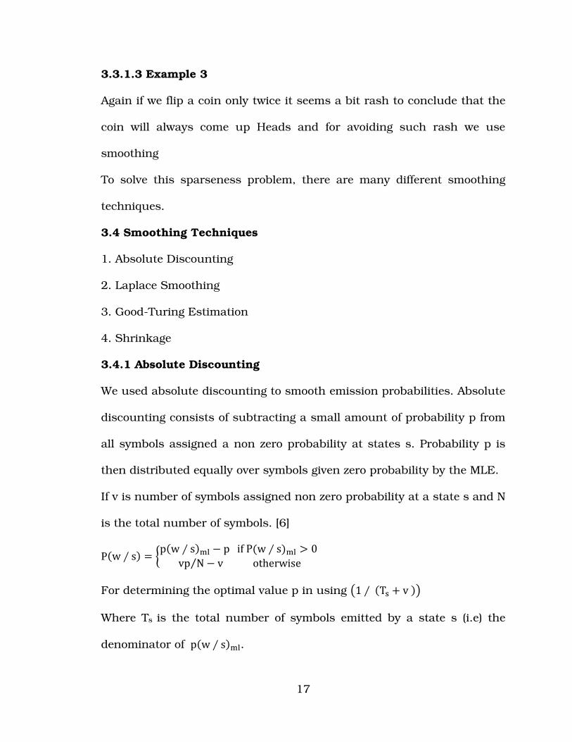
3.3.1.3 Example 3
Again if we flip a coin only twice it seems a bit rash to conclude that the
coin will always come up Heads and for avoiding such rash we use
smoothing
To solve this sparseness problem, there are many different smoothing
techniques.
3.4 Smoothing Techniques
1. Absolute Discounting
2. Laplace Smoothing
3. Good-Turing Estimation
4. Shrinkage
3.4.1 Absolute Discounting
We used absolute discounting to smooth emission probabilities. Absolute
discounting consists of subtracting a small amount of probability p from
all symbols assigned a non zero probability at states s. Probability p is
then distributed equally over symbols given zero probability by the MLE.
If v is number of symbols assigned non zero probability at a state s and N
is the total number of symbols. [6]
P)w + s- � .p)w + s-�( 0 p if P)w + s-�( 1 0 vp N⁄ 0 v otherwise 8
For determining the optimal value p in using �1 + )T# : v -� Where Ts is the total number of symbols emitted by a state s (i.e) the
denominator of p)w + s-�(.

18
3.4.2 Laplace Smoothing
It is also known as Add-One Smoothing, In Laplace Smoothing we have
to add some of the probabilities for unseen events
Take an example of flipping a coin. If we flip the coin twice and
count the number of Heads (H) and Tails (T), if heads come up both the
times the the probability for tails is zero. To avoid such situations we use
smoothing. To estimate the value p in Laplace Smoothing we have to
estimate p=)�;<-
)=>=?@ ABCDEF >G G@HIJ;|L|-
P=(1+2) ⁄ (2+2)=0.75
This rule is equivalent to starting each of our counts at one rather than 0
this is known as Laplace smoothing.
To avoid estimating any probabilities to be zero for events never observed
in the data we do the following in Laplace smoothing
P)w + s-@?I � )M)w, s- : 1- + )M)N- : OVO- where │V│ is the vocabulary size.
N (w,s)=number of times symbols w is emitted at state s
N(s) =Total number of symbols emitted by state s.
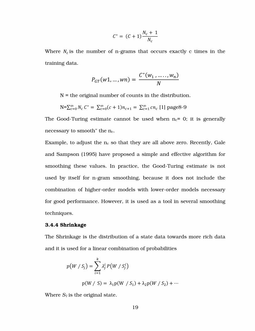
3.4.3 Good-Turing Estimation
The Good-Turing estimate (Good, 1953) is central to many smoothing
techniques. The general idea of the good turing is reallocate the
probability mass of n-grams that occurs c times.
For each count c, we should pretend that it occurs c* times
19
QR � )Q : 1- MS : 1MS
Where MS is the number of n-grams that occurs exactly c times in the
training data.
TUV)W1, … , WX- � QR)W� , … . . , WA-M
N = the original number of counts in the distribution.
N=∑ MSZS�[ QR � ∑ )\ : 1-XS;� � ∑ \XSZS��ZS�[ [1] page8-9
The Good-Turing estimate cannot be used when nc= 0; it is generally
necessary to smooth" the nc.
Example, to adjust the nc so that they are all above zero. Recently, Gale
and Sampson (1995) have proposed a simple and effective algorithm for
smoothing these values. In practice, the Good-Turing estimate is not
used by itself for n-gram smoothing, because it does not include the
combination of higher-order models with lower-order models necessary
for good performance. However, it is used as a tool in several smoothing
techniques.
3.4.4 Shrinkage
The Shrinkage is the distribution of a state data towards more rich data
and it is used for a linear combination of probabilities
]�^ + _ � � � aHb
H��T�^ + _H�
p)W + S- � λ�p)W + _�- : λep)^ + _e- : f Where S1 is the original state.

20
j is the state and i is the shrinkage ancestor
S2 is the larger context.
λ=shrinkage prior
In smoothing techniques the range of the shrinkage influence is when it
is used for context distributions not only towards those states but also
towards similar states with more data. They are three variants of
shrinkage used in smoothing techniques.

21
CHAPTER 4
IMPLEMENTATION
In thesis implementation we first discuss about the MLE. Before telling
about the MLE we will learn supervised learning.
4.1 Supervised Learning
The easiest solution for creating a model λ is to have a large corpus of
training examples, each annotated with the correct classification. If we
having such tagged training data we use the approach of supervised
training. In supervised learning we count frequencies of transmissions
and emissions to estimate the transmission and emission probabilities of
the model λ.
4.1.1 Maximum Likelihood Estimation (MLE)
MLE is a supervised learning algorithm. In MLE, we estimate the
parameters of the model by counting the events in the training data. This
is possible because the training examples for a MLE contain both the
inputs and outputs of a process. So we can equate inputs to
observations, and outputs to states and we easily obtain the counts of
emissions and transitions. These counts can be used to estimate the
model parameters that represent the process.
aij = # >G =F?AJH=H>AJ GF>C H => ` HA =hE J?CI@E i?=?
=>=?@ # >G =F?AJH=H>A GF>C =hE J=?=E H HA J?CI@E i?=?
bi (jb) = # >G ECHJJH>AJ >G =hE JkCD>@ lm GF>C H HA =hE J?CI@E i?=?
=>=?@ # >G ECHJJH>AJ GF>C =hE J=?=E H HA J?CI@E i?=?
22
There is a possibility of aij or bi (jb) being zero. for example consider the
case where state si is not visited by the sample training data then aij=0.
In practice when estimating a HMM from counts it is normally necessary
to apply smoothing in order to avoid zero counts and improve the
performance of the model on data not appearing in the training set.
In the thesis we implemented MLE using the function:
void CountSequence(char *seqFile); and
Parameters : tagged sequence file
Implementation of MLE involves accumulating the following counts
- count how many times it starts with state si
- count how many times a particular transition happens
- count how many times a particular symbol would be generated
from a particular state
- Implementation of MLE is shown in the followng fig

23
Figure 6 Algorithm Counting for in MLE
Using these count relative frequencies are computed to obtain
parameters of an HMM.
4.2 Laplace Smoothing
In Laplace smoothing we avoid zero probabilities for unseen events by
calculating the probability estimates using the following equations
Equation for smoothing emission probabilities
P)w + s-@?I � )M)w, s- : 1- + )M)N- : OVO- where │V│ is the vocabulary size.
N (w,s)=number of times symbols w is emitted at state s
N(s) =Total number of symbols emitted by state s.

24
Example:
If two times you toss a coin and head shows up twice
P(Head)lap=(2+1) / (2+2)=0.75
P(Tail)lap = (0+1)/(2+2) = 0.25
Equation for transition probabilities
N(si , sj): Number of times we move from state si to state sj
N(si): Number of transitions from state si
V: entire vocabulary (all output symbols)
aij= P(qt =sj / qt-1 = si) = (N(si , sj) + 1) / (N(si) + |V|)
In this thesis we implement Laplace Smoothing using function.
void Model::UpdateParameter(). Implementation of this function shown
below
Implementation on Laplace smoothing is show in figure.
Figure 7 Screen shot on Laplace smoothing

25
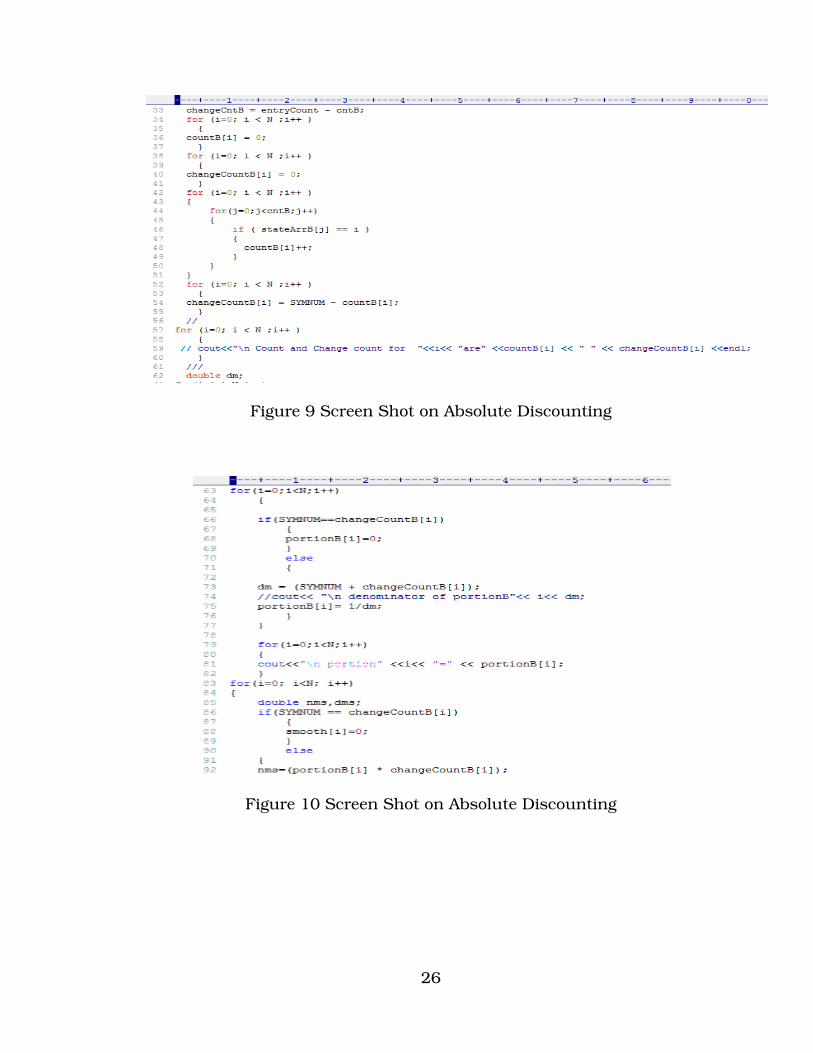
4.3 Absolute Discounting
We used absolute discounting to smooth emission probabilities. Absolute
discounting consists of subtracting a small amount of probability p from
all symbols assigned a non zero probability at states s. Probability p is
then distributed equally over symbols given zero probability by the MLE.
If v is number of symbols assigned non zero probability at a state s and N
is the total number of symbols. [6]
P)w + s- � .p)w + s-�( 0 p if P)w + s-�( 1 0 vp N⁄ 0 v otherwise 8
p)w + s-�( is emission probability.
V is the number of symbols assigned non zero probability at state s.
P= �1 + )T# : v -� Ts is the total number of symbols emitted by state s.
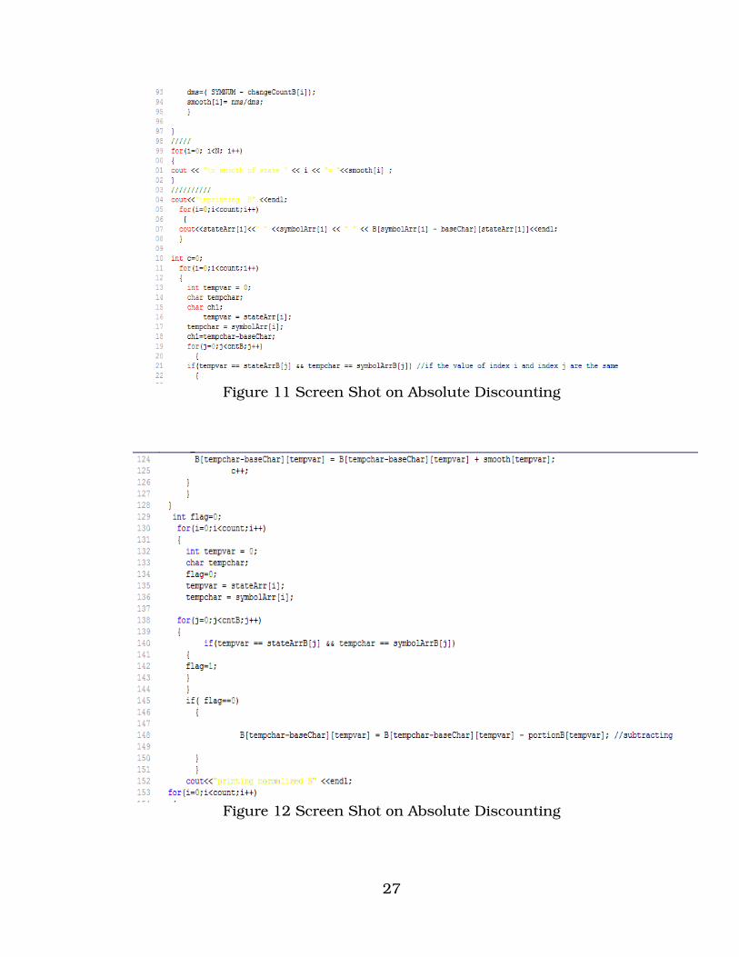
In the thesis we implemented Absolute Discounting using the function
Figure 8 Screen Shot on Absolute Discounting
26
Figure 9 Screen Shot on Absolute Discounting
Figure 10 Screen Shot on Absolute Discounting
27
Figure 11 Screen Shot on Absolute Discounting
Figure 12 Screen Shot on Absolute Discounting

28
Figure 13 Screen Shot on Absolute Discounting
We evaluated the performance of Laplace smoothing and Absolute
discounting by calculating precision and recall on the test data. The
results obtained are presented in chapter 5.

29
CHAPTER 5
RESULTS
5.1 Using HMM Model
An example will be provided in this chapter while training HMM model to
explain how it works on example data. In this HMM model, we have a
number of states, initial probabilities and output probability as shown in
figure 1.
5.1.1 HMM Model How it Looks
N is the number of states, InitPr is Initial probability, Output Pr is
Output Probability, TransPr is Transition Probability
Figure 14 HMM Model

30
5.1.2 Results on HMM and How it Works
To run this program we are taking a data of telephone numbers and
names.
The figure below shows the training data used in our example, a list of
phone numbers and names.
Figure 15 HMM Model Data
From this given data we have to find the state sequence made of 0 and 1
where 1 indicates phone numbers and 0 indicates characters other than
phone numbers. A continuous sequence of ten numbers is characterized
as a phone number.

31
Below figure shows about the training data and result of HMM on
telephone numbers and names. The output of HMM is a tagged sequence
file which looks like the one shown below.
Figure 16 HMM Train Data
After completing the execution on HMM we face some problem for unseen
events on MLE on state transition probabilities with given sequence for
observed symbols. For avoiding such situations we are using Smoothing
concept and different smoothing techniques.

32
5.2 Comparison of Two Smoothing Techniques
Laplace Smoothing and Absolute Discounting Smoothing are
implemented in this work. The definition and equation of MLE is
provided as below.
MLE is a Maximum Likelihood Estimation and while training HMM we
face some difficulties in Supervised Training
5.2.1 Equation on MLE
P (w ⁄ s)ml=(N(w , s)) ⁄ (N(s))
N (w, s) =number of times symbols w is emitted at state s
N(s) =Total number of symbols emitted by state s.
5.2.2 Equation on Laplace Smoothing
P)w + s-@?I � )M)w, s- : 1- + )M)N- : OVO- │V│ is the vocabulary size.
N (w,s)=number of times symbols w is emitted at state s
N(s) =Total number of symbols emitted by state s
There is a minute difference exist between equations of MLE and Laplace
Smoothing.
5.2.3 Equation on Absolute Discounting
P)w + s- � .p)w + s-�( 0 p if P)w + s-�( 1 0 vp N⁄ 0 v otherwise 8
There is no optimal value of p but we can determine p using �1 + )T# : v -� which often gives good results.
Where Ts is the total number of symbols emitted by a state s (i.e) the

33
denominator of p)w + s-�(.
5.3 Results on Laplace Smoothing
After including Laplace Smoothing in HMM, we see the count sequences
values for given. In Figure 4 we see the improvements on output
Figure 17 Laplace Smoothing Result
Here in this Figure 4(a) we see the initial state probabilities with states 0
is 1. In Figure 4(b) we see the Laplace Smoothing with two states 0 and 1
we get the sum B of state 0 as 1. In Figure 4(c) we can see the sum B of
state 1 is 1

34
Figure 18 Laplace Smoothing Result
Figure 19 Laplace Smoothing Result
5.4 Results on Absolute Discounting
After including the absolute discounting in HMM we see the initial
probabilities and state transition with states 0 and 1

35
Figure 20 Absolute Discounting Result
For reducing unseen events in HMM we include Smoothing Techniques
in HMM training as shown in above Figures. Now we have to calculate
the precision, recall and harmonic average accuracy for individual
smoothing techniques to see their effect on HMM.
The performance of the smoothing techniques is evaluated based on
standard precision, recall and harmonic average accuracy values [11].
Let TP be the number of true positives i.e. the number of documents
which both experts and HMM agreed as belonging to the phone category.
Let FP be the number of false positives i.e. the number of documents that
are wrongly tagged by the HMM as belonging to the tagged sequence.

36
5.5 Precision is defined as
precision � TPTP : FP
Let FP be the number of False Positive.
5.6 Recall is defined as
recall � TPTP : FN
Let FN be the number of False Negative.
5.7 Harmonic Mean
The harmonic mean of precision and recall is called the F1 measure is
defined
F1=e
rstuvwxwyz; r
tuv{||
Here In this work, we have to calculate the precision, recall and F1
values are calculated. The ideal values of precision and recall is
something which is greater than 0.8 and harmonic mean should be close
to 1.
5.8 Results on Evaluation
After careful calculations on HMM, without using Smoothing techniques
and including smoothing techniques we have got the following results of
the testing parameters:
5.8.1 Without Using Smoothing Techniques
Precision: 81.05
Recall: 98.54
FI: 89.68%
37
5.8.2 Using Smoothing Techniques
5.8.2.1 Laplace Smoothing
Precision: 86.05
Recall: 98.03
F1:91.7%
5.8.2.2 Absolute Discounting
Precision: 90.16
Recall: 99.8
F1: 95.2%

38
CHAPTER 6
CONCLUSIONS AND FUTURE WORK
In this work, we have measured the performance of two different
Smoothing Techniques in HMM for a given training data of phone
numbers. We also compared to performance without being used the
Smoothing Techniques. The accuracy of the HMM without using any
Smoothing was found to be 89.68 %. Laplace Smoothing in HMM had an
accuracy of 91.7% where as Absolute Discounting had 95.21 %. The
absolute discounting technique of HMM showed better accuracy
compared to Laplace Smoothing.
In future work, it might be interesting to implement other
smoothing techniques and compare their effect on the performance of the
HMM. Smoothing techniques that gave the best results may be used in
our HMM to improve the performance of HMM (Hidden Markov’s Model).
39
BIBLIOGRAPHY
1. Stanley F. Chen, Joshua Goodman, “An Empirical Study of Smoothing
Techniques for Language Modeling”, July 24,1998
2. ChengXiang Zhai, “A Brief Note on the Hidden Markov Models
(HMM),” March 16,2003
3. Chuan Liu, “cu HMM: a CUDA Implementation of Hidden Markov
Model Training and Classification”, May 6, 2009
4. Phil Blunsom, “Hidden Markov Models”, August 19, 2004
5. Lawrence R. Rabiner, “A Tutorial on hidden Markov Models and
Selected Applications in Speech Recognition”
6. Kazem Taghva, Jeffrey Coombs, Ray Pereda, Thomas Nartker,
“Address Extraction Using Hidden Markov Models”
7. Barbara Resch, “Hidden Markov Models”
8. L.E.Baum and T. Petrie, “Statistical Inference for Probabilities
function of Finite State Markov Chains”. Annals of Mathematical
Statistics, 37:1559-1563, [BP66], 1966
9. Gabor Molnar-Saska, “Analysis of the Maximum-Likelihood
Estimation of Hidden Markov Models”
10. Michael Buckland, Fredric Gey, “The relationship between Recall
and Precision”, University of California, Berkeley, Berkeley

40
VITA
Graduate College University of Nevada, Las Vegas
Sweatha Boodidhi
Degrees: Bachelor of Technology in Information Technology, 2007 Jawaharlal Nehru Technological University, India
Thesis Title: Using Smoothing Techniques to Improve the Performance of Hidden Markov’s Model
Thesis Examination Committee: Chairperson, Dr. Kazem Taghva, Ph.D. Committee Member, Dr. Ajoy K. Datta, Ph.D. Committee Member, Dr. Laxmi P. Gewali, Ph.D Graduate College Representative, Dr. Venkatesan Muthukumar, Ph.D