Paper PH300

Using SAS to Assess Dose Proportionality in Dose Escalation Studies

Keith Dunnigan, Mallinckrodt/Tyco Healthcare, St. Louis, MO

ABSTRACT Dose escalation studies provide a good opportunity to assess the linearity of PK parameters. This paper describes hypothesis testing and confidence interval (C.I.) methods for assessing dose proportionality based on linear regression and weighted least squares (WLS) linear regression. SAS® code is presented using an example study and AUCinf data. INTRODUCTION It is common within the pharmaceutical industry to conduct a parallel group, dose ranging study early in the drug approval process to establish a range of safe doses for the compound. This also offers an excellent chance to evaluate the linearity or dose proportionality of the PK parameters. In this paper we mention available statistical methods and describe and present SAS® code for using the Linear and WLS Linear regression methods to assess the dose proportionality of pharmacokinetic (PK) parameters. The data analyzed will be AUCinf data from an example dose escalation study in which forty eight subjects were randomized into 8 dosing groups of 6 each. SURVEY OF METHODOLOGY Within the pharmaceutical industry a variety of different methods have been used to assess dose proportionality. Common among these are methods based on the analysis of variance (ANOVA), linear regression (with and without intercepts), and the power model (regression of logS on logD). Weighted least squares (WLS) may also be used in conjunction with the regression approaches. Similar techniques are used for both parallel and crossover designs, though crossover experiments will usually involve repeated measures or mixed model modifications. Methods described here reference parallel studies only. Regardless of the model used, assessment of dose proportionality has generally evolved around hypothesis tests of the model parameters. Recently however some have pointed out that dose proportionality is fundamentally an estimation problem and have proposed basing proportionality assessment on confidence intervals and equivalence regions (Smith, 2000). With the exception of the ANOVA model, both the hypothesis test and confidence interval approaches have been principally used as overall tests of dose proportionality. That is, for a given dose range they make an overall conclusion about dose proportionality. The ANOVA approach has also allowed assessing proportionality on a dose by dose basis, but has the disadvantage being much less powerful since it doesn’t use the dose ordering information. In the presented example parallel study I have also introduced proportionality assessment based on using a weighted least squares (WLS) linear regression model and calculating confidence intervals on the mean value of the PK parameter estimates at each dose. This allows us to use the dose ordering information, assess linearity on a dose by dose basis, and overcome the homogeneity of variance objection commonly raised against the linear regression model. When model assumptions are met, this approach may be favorable for analyzing dose dependent PK parameters. I have also extended the overall confidence interval method by presenting results for dose independent pk parameters. The linear regression and WLS

linear regression models will be briefly summarized along with their traditional testing methods of assessment. Confidence interval techniques will then next be described, followed by a data analysis example with SAS code. STATISTICAL MODELS LINEAR REGRESSION The simple linear regression model is described by:

Si = β0 + β1Di + εi Where Si represents the value of the PK parameter at the ith dose and εi is the normally distributed error with standard deviation σi. To assess the dose proportionality using linear regression, hypothesis tests are traditionally performed on the intercept and slope parameters. If the slope is significantly greater than zero and the intercept is not significantly greater than zero then proportionality is assumed. Linear regression is also used to analyze dose independent PK parameters where dose independence is being analyzed by testing the ‘flatness’ of the response. If the slope is not significantly greater than zero then proportionality is concluded. WEIGHTED LEAST SQUARES (WLS) LINEAR REGRESSION Often in response (PK parameter) versus dose curves the variance of the data is seen to increase with increasing dose. This violates one of the primary assumptions behind the simple linear regression analysis and causes inaccurate pvalues and confidence intervals to be calculated for regression parameters and other model based estimates. Weighted least squares (WLS) is a method for transforming a linear regression analysis in order to correct for a non-constant error variance. Consider the case of the simple linear regression described earlier, where the usual regression assumptions require σi to be constant from dose to dose. A non-constant error variance can be stabilized everywhere by dividing both sides of the equation through by σi:

ii1

i0

i

i 1Sσε

σβ

σβ

σiiD ++=

It can be seen that the error term, εi/σi, has a constant variance of 1 for all doses and that the same regression coefficients are estimated in both the transformed and untransformed equations. Thus accurate confidence intervals and pvalues can be calculated for β0 and β1 as well as mean and prediction intervals for Si by using the transformed model. In practice σi is estimated by si, the sample standard deviation of the response at each dose. This transformation can be shown to be equivalent to a weighted least squares with weight = 1/ σi

2. For more details on WLS see Bowerman & O’Connell, Draper & Smith. ASSESSING DOSE PROPORTIONALITY CONFIDENCE INTERVAL APPROACH Once a good appropriate statistical model has been has been fit it may be used to assess dose proportionality. Traditionally hypothesis tests are performed on estimated model parameters using pvalues. More recently some have also proposed and used equivalence tests for assessing overall dose proportionality based on computing confidence intervals and comparing to equivalence regions. This approach will be described briefly for the linear regression model (for a more detailed description see Smith, 2000). In addition dose by dose C.I. methods for the linear regression will be introduced. If we denote the value of a PK parameter at the lowest study dose L by SL and at the highest dose H by SH then if the parameter is dose proportional:

LHL

H SLHS,

SS

==kLkH

where k is some constant. If we allow SH to deviate from true proportionality by a percentage ∆, then:

)1(LH

SS

SLHS

LHS

L

H

LLH

∆±=

∆±=

For dose independent PK parameters by definition the ratio of high to low dose is one and the equation becomes:

∆±=1SS

L

H

OVERALL C.I. APPROACH FOR LINEAR REGRESSION Dose Dependent Parameters Under the assumptions of the linear regression model and dose proportionality:

∆±=++

++

=∆±= 1HL,)1(

LH

SS

10

10

10

10

L

H

LH

LH

ββββ

ββββ

If we define the lower limit of our equivalence region by θL = 1 – ∆ and the upper limit as θH = 1 + ∆ then:

H10

10L θ

LββHββ

HLθ <

++

<

Completing the algebra shows (Smith 2000) that for any dose range of clinical interest the equivalence region can be expressed as:

( ) ( )L

L

1

0

H

H

Hθ-L1θHL

Hθ-L1θHL −<<−

ββ

To test overall dose proportionality using the C.I. approach we calculate the confidence interval for β0/β1, if it is entirely contained within the equivalence region then we conclude dose proportionality. This confidence interval can be calculated either by bootstrapping or by using Fieller’s Theorem (Finney 1978, p28). Dose Independent Parameters Under the assumptions of the linear regression model and dose independence:

H10

10L

10

10

L

H θLββHββ

θ,1SS

<++

<++

=∆±=LH

ββββ

Looking at the right side of the inequality we get:

Lθ-H1θ

ββ

1θL)θ-H(ββ

,0L)θ-(Hβ)θ1(β

L,βθβθHββ

H

H

0

1

HH0

1

H1H0

1H0H10

−<

−<

<+−

+<+

Where H/L > Hθ (true for any range of clinical interest). Similarly for the left side:

)Lθ-H()1(θ

ββ

β)Lθ-H(β)1(θ

HββLβθβθ

L

L

0

1

1L0L

101L0L

−>

<−

+<+

Where H/L > Lθ . Finally putting both sides together:

HH

H

0

1

L

L θLH where,

Lθ-H1θ

ββ

)Lθ-H()1(θ

>−

<<−

The confidence interval for β1/ β0 must be estimated by bootstrapping, since Fieller’s Theorem is unstable when the slope of the line is near zero. DOSE BY DOSE C.I. APPROACH FOR LINEAR & WLS LINEAR REGRESSION A linear regression model gives an equation for predicting an individual response, or the mean of an individual response at any dose. A standard result of linear regression is the confidence interval for the mean prediction at any specified dose (Bowerman & O’Connell, Draper & Smith). For a simple linear regression this is given by:

∑=

−

−+± n

1i

2i

202-n

2i

)x(x

)x(xn1sty α

Where x is the value of the ith dose, iy is the PK estimate at dose i, n is the total sample size, and s is the root mean squared error. To conform to standard practice (as in average bioequivalence) we compute confidence intervals about the mean of a prediction at each dose level rather than about an individual prediction. This is especially appropriate in a parallel design (where each subject is measured at only one dose level), since subject to subject variability is a major factor in PK analyses.

EQUIVALENCE & CONFIDENCE INTERVAL SPECIFICATION- OVERALL The equivalence limits θH, θL, or ∆ must be chosen for each study. Also the alpha level of the confidence interval must be chosen. As mentioned earlier there are no generally accepted rules for doing this. Much of what has been done to this point has borrowed from the standard practices used in bioequivalence studies (90% confidence intervals and θL, θH = 0.8, 1.25). The statistical development in bioequivalence centers around testing hypotheses based on the ratio of two normally distributed random variables or the difference of two lognormally distributed random variables. However, the development of proportionality models and tests is different from that in bioequivalence. Thus further study is needed regarding appropriate alpha levels for the confidence intervals of β1 (the power model) or for β0/β1 (the linear regression model). It is not immediately apparent that the 90% C.I. is appropriate. A 95% C.I. may be reasonable. In these data analyses we have computed both 90% and 95% C.I.’s for the overall proportionality assessments. EQUIVALENCE & CONFIDENCE INTERVAL SPECIFICATION- OVERALL – DOSE BY DOSE For the dose by dose analyses we have calculated equivalence regions for the linear regression analyses by first calculating an ‘ideal’ model which has perfect dose proportionality, then forming an equivalence interval at each dose by adding or subtracting 20% to the value predicted by this ideal model. The ‘actual’ model is used to compute 95% confidence intervals at each dose. If the ‘actual’ 95% confidence interval is entirely contained within the ‘ideal’ equivalence interval then we conclude proportionality at that dose. The ideal model was constructed by fitting a least squares line through the origin (i.e., a simple linear regression with no intercept). If the 95% C.I. for the least squares mean at a specified dose is entirely within the equivalence interval then we conclude dose proportionality at that dose. We may conclude that there is not overall dose proportionality, but that there is dose proportionality over a certain range of doses if we conclude proportionality at every dose within that range. DATA ANALYSIS These dose proportionality analysis methods will now be illustrated for case of the linear and WLS linear regression models using AUCinf data from an example study involving a narcotic compound. This example dose escalation study involves 8 dosing groups of 6 subjects each for a total of 48. In general several different statistical models may be fit and evaluated in each analysis. However it is really only necessary to find one, good fitting model. Since all statistical models are actually only approximations to reality, there may be none, one, or several different models that fit the data reasonably well. The goal of proportionality analysis is not to find the exact mathematical curve per se, but to quantify the degree to which our data follows or does not follow a straight line with no slope. To this end then we will require a good fitting model, but having found that we will in general be satisfied and not necessarily concerned with finding the perfect curve (for example issues such as interpretation, parsimony, and ease of calculation may weigh more heavily than tiny RSquare improvements in esoteric models). We will call a good fitting model one where the regression assumptions are largely satisfied, since statistical inference (i.e., accurate confidence intervals and pvalues) will depend on the validity of the model assumptions. STATISTICAL MODEL EVALUATION A scatter plot of AUCinf versus dose for the compound in this example study is shown in Figure 1. From these plots it can be seen that the linear regression is reasonable. The variance is seen to increase with dose. This seems to make the WLS regression model a good modeling candidate and a weighted least squares regression is performed with the weights equal to the reciprocal of the sample variance at each value of dose. The resulting residual plots and histogram are shown in Figures 2 and 3 revealing the much better fit of the WLS linear regression model over the unweighted regression model. The residuals are reasonably normal and their variance has been well equalized.

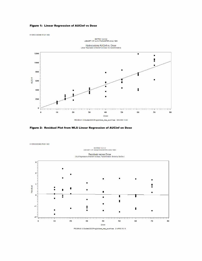
Figure 1: Linear Regression of AUCinf vs Dose

Figure 2: Residual Plot from WLS Linear Regression of AUCinf on Dose

Figure 3: Residual Histogram from WLS Linear Regression of AUCinf on Dose

ASSESSING DOSE PROPORTIONALITY Dose proportionality was assessed in 3 different ways: (1) On an overall basis by examining the pvalues for β0 and β1 (pvalue approach), (2) On an overall basis by calculating a confidence interval for β0/ β1 and comparing to an equivalence region, and (3) On a dose by dose basis by calculating confidence intervals for the mean of a prediction at each dose, then comparing with equivalence regions calculated at each dose level. For (2) above the confidence interval for β0/ β1 was calculated two ways: (i) by bootstrapping and (ii) by using Fieller’s Theorem. For (3) above the equivalence regions were formed by calculating a least squares regression line through the origin, then adding or subtracting 20% to the value predicted by the new line. The study data consisted of 48 subjects in 8 dosing groups of 6 subjects each. Bootstrap subsamples of n=24 were constructed by randomly sampling 3 subjects each from the 8 dosing groups. One thousand such subsamples were obtained and bootstrap confidence interval estimates obtained from the appropriate upper and lower percentiles. RESULTS The principle results from the model fitting and dose assessment analyses for the AUCinf PK parameter are presented in Table 1. Since the WLS linear model best fits the regression assumptions, the confidence interval techniques were only applied to this model. Using the pvalue assessment approach with the linear model would conclude proportionality. The intercept test does not reject the null hypothesis of no intercept (p=0.9761). For the WLS model proportionality would also be concluded as the slope tests different than zero (p<0.0001) and the intercept is not proved to be different than zero (0.9641). Using the overall confidence interval approach we can see that both the 90% bootstrap C.I. and the 90% Fieller’s F.I. would conclude dose proportionality. At the 95% level the bootstrap interval just does conclude proportionality while the Fieller’s misses a bit on the left side (F.I.=-1.93, 2.22; E.I.=-1.89, 0.04). Finally using the dose by dose approach and the 95% C.I.’s for the mean response at each dose we can see that

the C.I.’s are well contained within the equivalence intervals at all 8 doses, for both methods of calculating equivalence intervals. The individual C.I.’s seem especially convincing and we conclude that based on this model AUCinf is dose proportional.

Table 1: SUMMARY OF DOSE PROPORTIONALITY ANALYSES FOR AUCinf

Regression Model Parameter Estimates Intercept Linear

Regression

Model

RSquare B0 Pvalue a B1 Pvalue a

Linear 0.7694 -1.31117 0.9761 12.79582 <.0001 WLS 0.9613 -0.59014 0.9641 12.75758 <.0001

Confidence Interval Assessments – Overall

Parm (β0/ β1)

Conf (%)

Bootstrap C.I. Fieller’s F.I. Equiv Limits

Low High Low High Low High -0.046 90% -1.61 1.65 -1.64 1.81 -1.892 3.043 -0.046 95% -1.89 1.96 -1.93 2.22 -1.892 3.043

Confidence Interval Assessments – By Dose

Estimate

C.I. for Mean

Equiv Limitsb

C.I. for Mean (% of Ideal

Est) Dose (Ideal) (Model) Low High Low High Low High

10mg 127.6863 126.9857 110.73 143.24 102.149 153.2236

-13.3% 12.2%

15mg 191.5295 190.7736 176.61 204.93 153.2236 229.8353 -7.8% 7.0% 20mg 255.3726 254.5615 239.20 269.92 204.2981 306.4471 -6.3% 5.7% 30mg 383.0589 382.1373 357.54 406.73 306.4471 459.6707 -6.7% 6.2% 40mg 510.7452 509.7131 472.69 546.74 408.5962 612.8942 -7.5% 7.0% 50mg 638.4315 637.2889 586.95 687.63 510.7452 766.1178 -8.1% 7.7% 60mg 766.1178 764.8647 700.88 828.85 612.8942 919.3414 -8.5% 8.2%

WLS

70mg 893.8041 892.4405 814.65 970.23 715.0433 1072.565 -8.9% 8.6% a H0: Parameter = 0 b Limits are +/- 20% of estimate obtained from ideal line. The ideal line is a regression line with no intercept. SAS CODE USED IN DOSE PROPORTIONALITY ASSESSMENTS Pvalue based assessments First the simple linear regression and weighted linear regression models are ran. The data is contained in the dataset pkparm. The i option in the weighted regression gives the elements of the (XX’)-1 matrix which are required for calculating the Fieller’s C.I. later. The output dataset provides the C.I.’s for the mean value of AUCinf at each dose level used later in the dose by dose C.I. assessments. /********************************************************************* ** Input dataset pkparm has variables: ** ** ID - Subject ID ** Dose - Doseage subject received ** result - AUCinf PK parameter value ** Lresult - Log of result value ** ** There are 48 subjects, 6 subjects each in 8 Doseage groups(10,15, ** 20,30,40,50,60 and 70mgs) ***************************************************************/ ** Regular regression.;

proc reg data = wls alpha = 0.05; model result = dose; run; quit; ** WLS regression.; proc reg data = wls alpha = 0.05; model result = dose / i; weight wgt; output out = wlsout predicted = yhat residual = resid lclm = lcl_mean uclm = ucl_mean; run; quit; Overall Confidence Interval based assessments First the 90 and 95% Fieller’s Intervals are calculated: /*********************************************************************** ** 95% Confidence interval using Fieller's Theorem ***********************************************************************/ data fthm; b0 = -0.59014; b1 = 12.75758; s = 1.02455; tscore = tinv(0.975,46); /* for 95% C.I. * tscore = tinv(0.950,46); /* for 90% C.I. */ v11 = 162.11976028; v22 = 0.4668408941; v12 = -7.334035609; a = b0; b = b1; m = a/b; g = (tscore**2) * (s**2) * v22 / b**2; w = m - (g*v12/v22); coef = tscore * s / b; x = v11 - (2*m*v12) + (m**2) * v22; y = g * (v11 - ( (v12**2) /v22) ); del = coef * ((x - y)**0.5); low = (w - del) / (1 - g); hi = (w + del) / (1 - g); run; title "95% Fieller's C.I. for bo/b1"; proc print data = fthm; run Then the bootstrapped C.I.’s are calculated : /*********************************************************** ** Create and run macro randsamp to draw bootstrap samples ************************************************************/ %macro randsamp (numsamps=); %do i = 1 %to %eval(&numsamps);

/****** Generate Boostrap sample i ********/ data pkparm2; set pkparm; randnum = ranuni(-1); run; proc sort data = pkparm2; by dose randnum; run; data pkparm3; set pkparm2; by dose randnum; index + 1; if first.dose then index = 1; run; data boot&i; set pkparm3; where index < 4; if dose = 10 then intercept_t1 = 1 / 22.1; if dose = 15 then intercept_t1 = 1 / 37.4; if dose = 20 then intercept_t1 = 1 / 69.5; if dose = 30 then intercept_t1 = 1 / 46.9; if dose = 40 then intercept_t1 = 1 / 182.7; if dose = 50 then intercept_t1 = 1 / 129.3; if dose = 60 then intercept_t1 = 1 / 291.0; if dose = 70 then intercept_t1 = 1 / 189.5; wgt = intercept_t1**2; keep parm id dose wgt result lresult randnum index; run; /***** Generate bootstrap estimates of b0 and b1 from sample i ****/ ods output parameterestimates = parmest&i; ods listing close; proc reg data = boot&i; where parm = "AUCINF"; model result = dose / xpx i clb; weight wgt; run; quit; ods listing; data parmest&i.b; set parmest&i; keep variable estimate; run; proc transpose data = parmest&i.b out = parmest&i.c (drop = _label_ _name_); var estimate; id variable; run; data parmest&i.d; length sample $16.; set parmest&i.c; sample = "bootstrap&i";

ratio = intercept/dose; run; /***** Accumlate boostrap estimates into one dataset ******/ %if &i ne 1 %then %do; data parmest; set parmest parmest&i.d; run; %end; %else %if &i = 1 %then %do; data parmest; set parmest&i.d; run; %end; %end; %mend randsamp; /************************************************************************ ** Calculate boostrap confidence interval for bo/b1 with 1000 subsamples *************************************************************************/ data parmest; set aucinf_boot; run; ** Bootstrap C.I. for bo/b1; proc sort data = parmest; by ratio; run; data parmest2; set parmest; index + 1; pctl = index * 0.1; run; title "Bootstrap C.I. for bo/b1"; proc print data = parmest2 split = '_'; where index <= 60 or index >= 940; var sample intercept dose ratio pctl; label intercept = 'b0' dose = 'b1' ratio = 'b0/b1' pctl = 'Percentile'; run; Dose by Dose Confidence Interval Based Assessments First a regression with no intercept is fit to obtain the slope for the ideal line. Then the C.I.’s for the mean output from the WLS output is used to calculate the statistics for Table 1: ** Lin regression with no intercept.; proc reg data = wls; model result = dose / noint; run;

data wlsout2; set wlsout; yhat3 = 12.76863 * dose; /* Ideal line for perfect dose proportionality */ equiv2_lo = yhat3 - (0.2 * yhat3); /* 20% equivalence limits */ equiv2_hi = yhat3 + (0.2 * yhat3); pct2_l = ((lcl_mean / yhat3) * 100) - 100; pct2_h = ((ucl_mean / yhat3) * 100) - 100; pct2_lo = round(pct2_l,0.1); /* % C.I. Limits miss ideal */ pct2_hi = round(pct2_h,0.1); run; ** Output for Table 1.; title '95% Confidence Interval Assessments by Dose'; proc print data = wlsout2; var dose yhat3 yhat lcl_mean ucl_mean pct2_lo pct2_hi equiv2_lo equiv2_hi; run; CONCLUSION Since dose proportionality assessment is primarily an estimation problem, confidence/equivalence interval methods should be preferable to traditional testing approaches. The WLS linear regression model in combination with dose by dose Confidence/Prediction intervals may be an optimal method of establishing proportionality, especially for dose proportional PK parameters, and is easily implemented with SAS software. REFERENCES:

1. D.J. Finney. Statistical Method in Biological Assay, Third Edition, Charles Griffin & Company Ltd, London, 1978.

2. Smith BP, Vandenhende FR, DeSante KA, Farid NA, Welch PA, Callaghan JT, and Forgue ST.

Confidence Interval Criteria for Assessment of Dose Proportionality. Pharm Res 2000; 17:1278-1283.

3. K. Gough, M. Hutchison, O. Keene, B. Byrom, S. Ellis, L.Lacey, and J. McKellar. Assessment of

Dose Proportionality: Report from the statisticians in the pharmaceutical industry/pharmacokinetics UK joint working party. Drug Info. J. 29:1039-1048 (1995).

4. B. Bowerman and R. O’Connell. Linear Statistical Models: An Applied Approach, Second Edition,

PWS-Kent Publishing Company, Boston, 1990. 644-661.

5. Schuirmann, D.J. (1987) A Comparison of the Two One-Sided Tests Procedure and the Power Approach for assessing the Equivalence of Average Bioavailability. Proceedings of the Biopharmaceutical Section 121-126. American Statistical Association, Alexandria, VA.

6. Draper, N.R. and H. Smith. Applied Regression Analysis, John Wiley & Sons, New York, 1966.