using regression analyses for the determination of protein
TRANSCRIPT

Using Regression Analyses
For the Determination of Protein
Structure
From FTIR Spectra
A thesis submitted to
the University of Manchester for the degree of PhD
in the Faculty of Life Sciences
2014
Kieaibi Ellis Wilcox
CONTENTS
2
Table of Contents
Table of Contents ....................................................................................... 2
Table of Figures .......................................................................................... 6
List of Tables ............................................................................................ 14
List of Figures and Tables in Appendices .............................................. 16
Abbreviations ........................................................................................... 18
Abstract ..................................................................................................... 19
Declaration ................................................................................................ 20
Copyright Statement ................................................................................ 21
Acknowledgement .................................................................................... 22
1 Introduction ....................................................................................... 23
1.1 Protein Structure ........................................................................... 23
Primary structure .................................................................. 24 1.1.1
Secondary Structure .............................................................. 25 1.1.2
Tertiary structure .................................................................. 28 1.1.3
Quaternary Structure ............................................................ 29 1.1.4
Protein Fold ........................................................................... 30 1.1.5
1.2 Experimental Determination of Protein Structures ...................... 31
Vibrational Spectroscopy ...................................................... 32 1.2.1
Fourier Transformed Infrared (FTIR) ..................................... 32 1.2.2
1.3 Computational Analysis Theory .................................................... 38
Multivariate Analysis ............................................................. 39 1.3.1
Data Pre-processing .............................................................. 45 1.3.2
Validation of the model ........................................................ 52 1.3.3
Determination of the unknown ............................................ 53 1.3.4
1.4 Aim of this research ...................................................................... 53
Research Objectives .............................................................. 54 1.4.1

USING REGRESSION ANALYSES FOR THE DETERMINATION
OF PROTEIN STRUCTURE FROM FTIR SPECTRA 3
2 Experimental Method: ATR-FTIR spectroscopy .......................... 56
2.1 Introduction .................................................................................. 56
2.2 Sample preparation ...................................................................... 57
2.3 Spectral measurement and Processing ......................................... 57
Baseline Correction and Atmospheric Correction ................ 58 2.3.1
ATR correction....................................................................... 58 2.3.2
2.4 Data Pre-processing for Multivariate Analysis .............................. 60
Outlier Detection .................................................................. 62 2.4.1
Centring and Scaling. ............................................................. 64 2.4.2
Multiplicative Scattered Correction (MSC) ........................... 65 2.4.3
Standard Normal Variate (SNV) ............................................ 67 2.4.4
2nd Derivative ....................................................................... 68 2.4.5
2.5 Discussions .................................................................................... 70
3 PCA Protein Structure Classification ............................................. 73
3.1 Introduction .................................................................................. 73
3.2 Dataset used for this method ....................................................... 75
3.3 PCA Model ..................................................................................... 75
3.4 Model Validation ........................................................................... 77
3.5 Results and Discussion .................................................................. 78
3.6 Conclusion ..................................................................................... 94
4 PLS Regression for Protein Secondary Structure Determination97
4.1 Introduction .................................................................................. 97
4.2 Protein dataset used for this method ........................................... 99
Data Selection Scheme........................................................ 100 4.2.1
4.3 PLS Modelling .............................................................................. 101
4.4 Results and Discussions .............................................................. 103
Model Validation ................................................................. 106 4.4.1
Cross-Validation .................................................................. 106 4.4.2

CONTENTS
4
Independent Test Set .......................................................... 108 4.4.3
Coefficient of Determination (R2) ....................................... 109 4.4.4
PCR ...................................................................................... 110 4.4.5
PLS with 2nd Derivative ........................................................ 111 4.4.6
Zeta scores ζ ..................................................................... 115 4.4.7
PCR/PLS comparison ........................................................... 116 4.4.8
Results for Proteins in D2O .................................................. 119 4.4.9
4.5 Other PLS Applications ................................................................ 122
iPLS Method ........................................................................ 123 4.5.1
4.6 Results and Discussion ................................................................ 128
α-helix ................................................................................. 128 4.6.1
β-sheet ................................................................................ 130 4.6.2
4.7 Validation Set .............................................................................. 131
4.8 Conclusion ................................................................................... 135
5 Multivariate analysis of pH effect on α-lactalbumin ................... 137
5.1 Introduction ................................................................................ 137
5.2 Sample preparation .................................................................... 139
5.3 ATR-FTIR Spectroscopy ............................................................... 140
5.4 PLS and PCA Modelling Technique .............................................. 140
5.5 Results and Discussion ................................................................ 142
Inspection of the Amide I Spectral Plots ............................. 142 5.5.1
Amide I PLS Results ............................................................. 146 5.5.2
Inspection of the Amide II Spectral Plots ............................ 149 5.5.3
Amide II PLS Results ............................................................ 150 5.5.4
Inspection of the Amide III Spectral Plots ........................... 151 5.5.5
Amide III PLS Results ........................................................... 154 5.5.6
PCA of α-Lactalbumin Spectra ............................................ 155 5.5.7
Comparison with other methods ........................................ 158 5.5.8
USING REGRESSION ANALYSES FOR THE DETERMINATION
OF PROTEIN STRUCTURE FROM FTIR SPECTRA 5
5.6 Conclusion ................................................................................... 160
6 Limit of Quantitation of Protein Structure Using PLS ............... 163
6.1 Introduction ................................................................................ 163
6.2 Sample preparation .................................................................... 165
6.3 FTIR Spectroscopy ....................................................................... 165
6.4 PLS Model.................................................................................... 166
6.5 Results and discussion ................................................................ 167
6.6 Conclusion ................................................................................... 180
7 Conclusion ....................................................................................... 182
8 References ........................................................................................ 188
Appendix A ............................................................................................. 209
Appendix B ............................................................................................. 213
Appendix C ............................................................................................. 225
Appendix D ............................................................................................. 230
46,795 words

CONTENTS
6
Table of Figures
Figure 1.1. This is a diagrammatic representation of the peptide
bond of amino acid residues and the backbone angles
that are formed; phi (Φ) for the angle between N-Cα, psi
(Ψ) for the angle between Cα-C bond, and omega (Ω) for
the angle between C-N bond. .............................................. 25
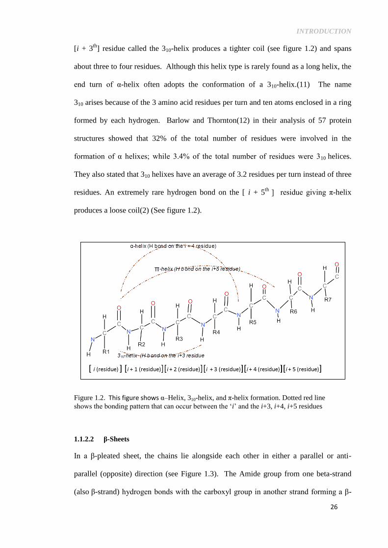
Figure1.2. This figure shows α–Helix, 310-helix, and π-helix
formation. Dotted red line shows the bonding pattern that
can occur between the ‘i’ and the i+3, i+4, i+5 residues ..... 26
Figure1.3. Parallel and anti-parallel β-Sheet formation ........................ 28
Figure1.4. Electromagnetic Spectrum. frequency (ν) = speed /
wavelength(λ). The Mid- IR region of the spectrum is
the wavelength region between 3x10⁻⁴
and 3x10⁻³
cm or
about 4000 – 400 cm-1
in wavenumbers .............................. 33
Figure 1.5. A general schematic of an FT-IR spectrometer. .................. 35
Figure 1.6. This diagram illustrates the evanescent wave reaching
into the sample at 45° angle. This angle is called the
angle of incidence. ............................................................... 37
Figure 1.7. Diagrammatic representation of the generalized
multivariate equation represented in eq. 1.3. ‘Y’ is
predicted on the basis of ‘X ‘and in such a way that the
residual, ‘ε’ is minimized. ................................................... 41
Figure 1.8a-c. Figure 1.8a shows the original data points. Figure 1.8b:
shows the centred data which are the individual points
minus the mean of the data; this puts the new mean at 0,
making some of the data negative. Figure 1.8c. Scaled
data: data looks shortened and broadened in an attempt to
decrease group distance. This results in a zero mean and
unit variance of any descriptor variable. ............................. 47
Figure 1.9. Outlier plot showing a red dot as an outlier, which
clearly does not correlate with the rest of the data. ............. 50
Figure 2.1a. Blue spectrum of fibrinogen is ATR-corrected to attain
the correct Amide I:Amide II band ratio of its
transmission counterpart. ..................................................... 59
Figure 2.1b. Amide I – Amide II transmission band ratio is not totally
attained by the ATR corrected carbonic anhydrase
spectrum (in Blue). .............................................................. 59
Figure 2.2a. ATR-FTIR Spectra of the 90 proteins in H2O solution
(spectra of the Amide I and Amide II region from
different instruments) before scaling, removal of outliers
and second derivative. ......................................................... 61

USING REGRESSION ANALYSES FOR THE DETERMINATION
OF PROTEIN STRUCTURE FROM FTIR SPECTRA 7
Figure 2.2b. ATR-FTIR Spectra of the 90 proteins in H2O solution
(spectra of the Amide I and Amide II region different
instruments) after normalization but before outlier
detection. ............................................................................. 62
Figure 2.3a. Outlier detection using mahalanobis distance. Plot
shows D-glucosamine (sugar) and Spectrin as outliers.
The mean of each spectrum and the standard deviation of
each sample are plotted on the x-axis and y-axis,
respectively .......................................................................... 63
Figure 2.3b. Distribution of protein samples after outliers were taken
out. ....................................................................................... 64
Figure 2.4. 84 scaled protein spectra (Amide I region) measured in
H2O ...................................................................................... 65
Figure 2.5a. MSC pre-processing performed on 84 raw data showing
reduction in spectral intensities. Spectra are pulled
towards the raw spectrum with the mean value................... 66
Figure 2.5b. MSC pre-processing performed on normalized spectra.
Spectra are pulled towards the normalized mean sample. ... 66
Figure 2.6a. SNV pre-processing performed on 84 protein spectra of
raw protein samples ............................................................. 67
Figure 2.6b. SNV pre-processing done on normalized 84 protein
spectra .................................................................................. 68
Figure 2.7. Second derivative on the normalized data of the ATR-
FTIR spectra of 84 proteins collected in H2O ..................... 69
Figure 3.1. PC plot of scaled data for the Amide I region of 84
spectra showing percentage variance of the first 4
principal components. The blue line in the plot indicates
the cumulative percentage variance for all 4 PCs. .............. 78
Figure3.2. PCA scores plot for Amide I region (1600 cm-1
–
1700cm-1
) of ATR-FTIR spectra of 84 proteins in H2O
(PC1xPC2). Plot shows the clustering of scores. Blue
dots are primarily α proteins, red dots are primarily β
proteins, green dots indicate proteins of other types ........... 80
Figure 3.3. Loading Plot of the Amide I (1600 cm-1
– 1700cm-1
)
region for spectra of 84 proteins in H2O This Plot shows
the clustering of scores. Wavenumbers of spectral
signals indicate the discriminating features associated
with clustering of scores in Figure 3.2. ............................... 81
Figure 3.4. PC1, PC2, and PC3 loadings plot of Amide I (1600 cm-1
– 1700cm-1
) region for spectra of 84 proteins in H2O
(PC1xPC2). The wavenumbers listed indicate the
discriminating features associated with clustering of
scores in Figure 3.2. Both Figure 3.3 and Figure 3.4
were combined in the analysis of the scores plot (Figure
3.2). ...................................................................................... 81

CONTENTS
8
Figure 3.5. PCA scores of ATR-FTIR spectra of proteins in H2O.
Plot highlights the clusters of mixed proteins; αβ proteins
(multi-domain) as green dots, α+β proteins (mainly anti-
parallel) as red stars, α/β proteins (mainly parallel) as
black stars. The little unlabelled blue and red dots are α-
helix and β-sheet proteins highlighted in Figure 3.2 ........... 84
Figure 3.6. Scaled ATR-FTIR spectra of the Amide I region for
ribonuclease S in red (which contains mainly anti-
parallel β-sheet), transketalose in blue (mainly parallel β-
sheet), and lactic dehydrogenase in green (contains both
parallel and anti-parallel β-sheet) ........................................ 85
Figure 3.7. PC2 loading spectra plot of the ATR-FTIR Amide I
region for 84 proteins in H2O. ............................................. 86
Figure 3.8. Biplot (PC scores and loadings) of Amide I region; blue
lines show the length of each loading and their
directions. Red dots are the protein sample scores. ............ 88
Figure 3.9. PC plot of Scaled Amide II region of 84 spectra showing
percentage variance of the first 4 principal components.
The blue curve indicates the cumulative variation of all 4
components .......................................................................... 90
Figure 3.10. Scores plot for Amide II region (1480 cm-1
– 1600cm-1
)
of spectra of proteins in H2O (PC1xPC2). Plot shows the
clustering of scores. Blue dots are primarily α-helix rich
proteins, red dots are primarily β-sheet rich proteins, and
green dots indicate proteins of other structural types .......... 92
Figure 3.11. Loading Plot of the Amide II (1480 – 1600cm-1
) region
of spectra for 84 proteins in H2O (PC1xPC2). Plot
shows the clustering of scores. Wavenumbers in the
plot, especially the extreme right and left numbers
indicate the discriminating wavenumbers associated with
clustering of scores in Figure 3.10. ..................................... 93
Figure 4.1. Schematic representation of samples used in the training
set and the test set after application of the Kennard Stone
selection algorithm. Matrix X represents the FTIR
spectra while vector ‘y’ represents the percentage
fraction of structure determined by DSSP analysis from
X-ray crystallographic data. This figure represents the
strategy for the 84 protein samples measured in H2O. ........ 101
Figure 4.2. Explained Y variance of α-helix for Amide I region;
explained variance is about 96% for 10 components. ......... 104
Figure 4.3. Plot shows Root Mean Square Error (RMSE) vs. number
of components for α-helix of the Amide I region. 10
components gave low root mean square error and was
chosen to fit the data. ........................................................... 104
Figure 4.4. Explained Y variance of β-sheet for the Amide I region
is about 95 % for 10 components. ....................................... 105
USING REGRESSION ANALYSES FOR THE DETERMINATION
OF PROTEIN STRUCTURE FROM FTIR SPECTRA 9
Figure 4.5. Root Mean Square Error for β-sheet analysis for the
Amide I region. .................................................................... 106
Figure 4.6. CV cross-validation: 4 PLS components only are
required to fit the α-helix model for proteins in H2O for
the Amide I region. .............................................................. 108
Figure 4.7. Residual plot of the 60 samples in the Amide I region.
Error levels between the fit and the individual data are
shown for each sample. Note: The residuals are not
sorted by protein but by the order in which they were
analysed. .............................................................................. 110
Figure 4.8. Performance of CV cross-validation: 4 PLS components
is optimal for PLS-CV while 5 components is optimal for
PCR-CV. .............................................................................. 111
Figure 4.9. The plot of the calibration set for the analysis of α-
helix content from Amide I region : This plot shows
PLS fitted vs response (X-ray crystallography values)
using the FTIR spectra of 60 proteins in H2O for
calibration. The red line of fit going through the origin
emphasises the positive correlation in the data. .................. 113
Figure 4.10. Test set plot for analysis of α-helix from the Amide I data:
PLS fitted vs response on 44 proteins in H2O used for
testing the model. The model shows the relationship
between the crystal structure values and the calculated
values of α-helix from FTIR spectra for these proteins. ..... 113
Figure 4.11. Plot shows PLS prediction for β-sheet vs. X-ray
crystallography vales used in the training of the Amide I
region. The training set had FTIR spectra of 60 proteins
in H2O. The red line of fit going through the origin
emphasises the positive correlation in the data. .................. 114
Figure 4.12. Test set plot of Amide I β-sheet: PLS fitted vs response
on 44 proteins in H2O used for testing the model. .............. 114
Figure 4.13. Plot of RMSECV vs. PLS component for the global
model. Component number 2 has the lowest RMSECV. ... 124
Figure 4.14a Each bar in the plot is a spectral interval. The plot shows
interval numbers 1-7 ; Interval number 5 corresponds to
frequency factors in the range 1641 cm-1
– 1628 cm-1
for
α-helix, The dotted line represents the RMSECV for the
global iPLS model. Numbers in italics in each interval
bar signifies the number of iPLS components used in
fitting each local model. See Table 4.3 for intervals and
wavenumber range. The curve in the background is a
spectrum of the Amide I region. .......................................... 125
Figure 4.14b. Plot shows interval number 6 (6th
bar) corresponding to
frequency factors in the range 1614–1627 cm-1
for β-
sheet. See Table 4.3 for each interval actual beginning
and ending wavenumbers). Dotted line is the RMSECV

CONTENTS
10
for the global iPLS model. The dotted line represents the
RMSECV for the global iPLS model. Numbers in italics
in each interval bar signifies the number of iPLS
components used in fitting each local model. The curve
in the background is a spectrum of the Amide I region. ..... 126
Figure 4.15a. Plot of the Amide I normalized spectral region shows the
spectral region (in grey bar) used for iPLS analysis of α-
helix structure. . The grey bar contains the most
variation for of α-helix structure. This region (1641–
1628 cm-1
) corresponds to interval number 5 from Table
4.14a. ................................................................................... 127
Figure 4.15b. Plot of the normalized spectral region of Amide I that
contain the most significant region (in grey bar) for β-
sheet structure. The grey bar contains the most variation
for β-sheet structure. This region (1627 cm-1
–1614 cm-1
) was assigned to interval number 6 from Figure 4.14b. ..... 127
Figure 4.16a. Prediction line of fit for α-helix from the iPLS global
model in the in Amide I region (1700 – 1600 cm-1
). 3
iPLS components were used for building the model. The
numbers in the plot represent the different proteins in the
dataset which are listed in Table 4.4 ................................... 129
Figure 4.16b. Prediction line of fit for α-helix from the iPLS local
model in the in Amide I region (1641 cm-1
– 1628 cm-1
).
3 PLS components were used for building the model.
The numbers in the plot are the different proteins in the
dataset which are named in Table 4.4. ................................ 129
Figure 4.17a. Prediction line of fit for β-sheet from the iPLS global
model in the Amide I region (1700 cm-1
– 1600 cm-1
). 3
iPLS components were used for building the model. The
numbers in the plot are the different proteins in the
dataset which are named in Table 4.4. ................................ 130
Figure 4.17b. Prediction line of fit for β-sheet from the iPLS local
model in the Amide I region (1627 cm-1
– 1614 cm-1
). 3
iPLS components were used for building the model from
the 6th
spectral interval. The numbers in the plot are the
different proteins in the dataset which are named in
Table 4.4. ............................................................................. 131
Figure 4.18a. Plot of local model line of fit for the prediction of α-helix
in Amide I (1641 cm-1
– 1628 cm-1
). 3 PLS components
for the 5th
spectral interval were used for the prediction
of proteins in the test set.. The numbers in the plot are
the different proteins in the dataset which are named in
Table 4.4 .............................................................................. 132
Figure 4.18b. Plot of local model line of fit for the prediction of β-sheet
in Amide I (1627 cm-1
– 1614 cm-1
). 3 PLS components
for the 6th
spectral interval were used for the prediction
of proteins in the test set. The numbers in the plot are the

USING REGRESSION ANALYSES FOR THE DETERMINATION
OF PROTEIN STRUCTURE FROM FTIR SPECTRA 11
different proteins in the dataset which are named in
Table 4.4. ............................................................................. 132
Figure 5.1. The diagram on the left of α-LA (PDB ID: 1HFZ) shows
the native structure of α-LA, the intermediate unfolded
state is shown in the middle and the unfolded state is
represented on the right. The PDB reported structure of
the bovine α-LA (1HFZ is 43% helical structure, 9% -
sheet, 48% other. The Ca2+
ions are shown in black, the
blue ribbon represents α-helix, the green ribbon
represents 310-helix and the green arrows represent β-
sheet 139
Figure 5.2. Normalized FTIR spectra of α-LA from pH 7.0 to pH 2.0
covering spectral region 1900 - 1000 cm-1
. ......................... 141
Figure 5.3 The normalized Amide I region of -LA shows the
changes and shifts in spectral peaks as pH decreases
from 4.0 to 2.0 ..................................................................... 142
Figure 5.4a. Plot of the second derivatives of the FTIR spectrum for α-
LA in the native state at pH 7.0. A peak at 1657-1658
cm-1
is clearly visible. The second derivatives for pH 6.5
and 6.0 (not shown) are very similar. .................................. 143
Figure 5.4b. The plot of the normalized spectra of α-LA at pH 6-7 and
the changes in the intensities and frequencies at about
1657 cm-1
. These spectra of pH 6.5 and pH 6.0 are
similar to the spectrum of pH 7.0 which is in the native
state. 144
Figure 5.5a. This figure shows well resolved second derivative of α-LA
in the pH 3.0 and pH 3.5; the second derivative spectrum
shows a peak at about 1657 cm-1
. The green spectrum
shows changes in intensity. ................................................. 145
Figure 5.5b. This figure shows well resolved second derivative of α-LA
at pH 2.0. The second derivative spectrum shows a peak
at about 1720 cm-1
. .............................................................. 145
Figure 5.5c. Plot of the normalized spectra of α-LA at pH 2.0-3.5 and
the shifts in the intensities and frequencies. ........................ 146
Figure 5.6. This plot highlights changes in the secondary structure of
α-LA as a function of pH, based on PLS analysis. The
horizontal axis values represents the pH values, the
vertical axis represents the secondary structure
proportions. Below pH 3.0, a gain in β-sheet and a loss
in α-helix is seen. The error bars were calculated from
the PLS result residual for each spectrum (which is the
observed X-ray value – the calculated FTIR value). ........... 149
Figure 5.7. The plot of the normalized spectra of α-LA at pH 2.0 -
7.0. Plot shows peak shift and structural changes
especially for pH 2.5 and pH 2.0 ......................................... 150

CONTENTS
12
Figure 5.8. This is the plot of the effect of pH 3.5 (intermediate) –
pH 2.0 on the normalized Amide I spectral region of α-
LA protein. Plot shows slight changes at these pH
levels. The different spectral colours represent different
pH levels. ............................................................................. 152
Figure 5.9. Plot of Amide III region depicts peaks shift for pH 5.5 -
pH 4.0 at 1250 cm-1
and pH 4.0 at 1279 cm-1
respectively. ......................................................................... 153
Figure 5.10. Plot of Amide III region depicts peak for pH 7.0 (native
protein) at 1256 cm-1
........................................................... 154
Figure 5.11. Score plot of α-LA at different pH on the first and
second principal components. Principal Component
Score plot shows the classification of α-LA spectra based
on the pH levels. PC1 has more native state spectra on
left and acidic state spectra on the right. PC2 separates
the intermediates at the top .................................................. 156
Figure 5.12. Loading plot shows the most significant wavenumbers
that contribute to the spectral discrimination seen in the
score plot in figure 5.13. ...................................................... 157
Figure 5.13. Loading spectra of PC1 and PC2 shows the most
significant wavenumbers that contribute to the spectral
discrimination seen in the score plot in Figure 5.11.
Both plots of Figure 5.12 and 5.13 were combined for
the analysis, but can be used separately. ............................. 157
Figure 6.1. The raw spectra of six proteins (β-Lactoglobulin, BSA,
fibrinogen, IgG, lysozyme, and ubiquitin) acquired at
200, 100, 50, 25, 12.5, 6.25, 3.13, 1.56, 0.78, 0.39, 0.19
mg/mL. ................................................................................ 166
Figure 6.2. Spectra of 66 proteins in the Amide I region in
concentrations between 200 mg/mL and 0.19 mg/mL and
scaled for PLS analysis. ....................................................... 168
Figure 6.3. Comparison of normalized spectra of Lysozyme at
concentration of 0.19 mg/mL, 50mg/mL and 200 mg/mL
in the Amide I region with major peak at 1654 cm-1
........... 169
Figure 6.4a. The second derivative spectra of the Amide I region of
IgG in aqueous solution at 200 mg/mL, 50 mg/mL and
0.19 mg/mL collected with FTIR spectroscopy .................. 170
Figure 6.4b. The normalized spectra of the Amide I region of IgG in
aqueous solution at 200 mg/mL, 50 mg/mL and 0.19
mg/mL collected with FTIR spectroscopy. ......................... 171
Figure 6.5. Plot of predicted α-helix content from FTIR spectra of
concentrations between 0.19 mg/mL and 200mg/mL in
comparison to the content measured from X-ray
crystallography. The Amide I region (1600 – 1700 cm-1
)
was used for the PLS analysis. ............................................ 179

USING REGRESSION ANALYSES FOR THE DETERMINATION
OF PROTEIN STRUCTURE FROM FTIR SPECTRA 13
Figure 6.6. Shows β-sheet structure predicted from FTIR spectra of
concentrations between 0.19 mg/mL and 200mg/mL vs.
X-ray crystallography. Amide I region (1600 – 1700 cm-
1) was used for the PLS analysis.......................................... 180

CONTENTS
14
List of Tables
.Table 2.1. A table of pre-processing methods and their minimum and
maximum values of spectral intensities...................................69
Table 3.1. PCA analysis for the Amide I region listing the
eigenvalues Sum of Squares, their percentage variance and
the cumulative variance. ..........................................................79
Table 3.2. PCA Table shows the eigenvalues Sum of Squares, their
percentage variance and the cumulative variance for the
Amide II region. ......................................................................91
Table 3.3. FTIR marker bands of protein classes in the Amide I
region. ......................................................................................96
Table 4.1a. Prediction results of PLS models of calibration and
validation sets for amide I, amide II, and amide I & II,
using Normalized + 2nd
derivative pre-processed data are
shown as grey highlights (rows 3,4 & 5). Results for PCR
and PLS methods on ‘Normalized + SNV’ are also shown
in the first and second row. For all methods, 60 protein
samples were used for calibration and for internal cross-
validation, 44 samples were used for independent test set. ...118
Table 4.1b. Prediction results of PLS models of calibration and
validation sets for amide I, amide II, and amide I & II,
using Normalized + 2nd derivative pre-processed data are
shown as grey highlights (rows 3,4 & 5). Results for PCR
and PLS methods on ‘Normalized + SNV’ are also shown
in the first and second row. For all methods, 60 protein
samples were used for calibration and for internal cross-
validation, 44 samples were used for independent test set.
– Continue from table 4.1a. ..................................................119
Table 4.2. Comparison of PLS results of the secondary structure of
proteins in H2O and D2O. The percentage secondary
structure for each protein derived from X-ray
crystallography served as a reference. ...................................121
Table 4.3. Table of intervals and their corresponding frequencies;
interval number 8 which covers the Amide I region was
used for the iPLS global model. ............................................126
Table 4.4. The list of proteins used for the both calibration and test
set in the iPLS. These proteins are listed to match the
numbers in the line of fit plot for both calibration and
validation for iPLS models. ...................................................133
Table 4.5. Table shows results for iPLS models for both global and
local regression analyses. Results of the traditional PLS
analysis of the Amide I region (1600-1700 cm-1
) are listed
for comparison. ......................................................................134
USING REGRESSION ANALYSES FOR THE DETERMINATION
OF PROTEIN STRUCTURE FROM FTIR SPECTRA 15
Table 5.1. PLS prediction results for the secondary structure content
of Amide I region of α-lactalbumin at different pH levels
using normalized and 2nd
derivative pre-processed data.
Structural values are presented as proportions calculated
from 1HFZ (pH 8.0) file using DSSP script. .........................148
Table 5.2. PLS Prediction results for the secondary structure of
Amide II region of α-LA at different pH levels using
normalized and 2nd
derivative pre-processed data.
Structural values are presented in proportions. .....................151
Table 5.3. PLS Prediction results for the secondary structure content
of Amide III region of α -lactalbumin at different pH
levels using normalized and 2nd
derivative pre-processed
data. Structural values are presented in proportions. ............155
Table 6.1. PLS results of α-helix content of 6 proteins. FTIR spectra
were used for this analysis. Each protein spectra was
collected at concentrations ranging from 0.19 mg/mL to
200 mg/mL. ...........................................................................174
Table 6.2. PLS results of β-sheet content of 6 proteins. FTIR spectra
were used for this analysis. Each protein spectra was
collected at concentrations ranging from 0.19 mg/mL to
200 mg/mL. ...........................................................................175
Table 6.3. PLS results of 310-helix content of 6 proteins. FTIR
spectra were used for this analysis. Each protein spectra
was collected at concentrations ranging from 0.19 mg/mL
to 200 mg/mL. .......................................................................176
Table 6.4. PLS results of Turns content of 6 proteins. FTIR spectra
were used for this analysis. Each protein spectra was
collected at concentrations ranging from 0.19 mg/mL to
200 mg/mL. ...........................................................................177
Table 6.5. PLS results of Disordered content of 6 proteins. FTIR
spectra were used for this analysis. Each protein spectra
was collected at concentrations ranging from 0.19 mg/mL
to 200 mg/mL. .......................................................................178
Table 6.6. R2 and RMSE (δ) of PLS analysis of secondary structure
contents determined from FTIR spectra in the Amide I
regions. ..................................................................................179
CONTENTS
16
List of Figures and Tables in Appendices
Figure C1. Principal Component plot of Amide I region of 16 proteins
in D2O showing percentage variance of the first 4 PCs.
Blue line indicates that the accumulative percentage
variance is about 98%. ......................................................... 226
Figure C2. PCA Score plot of the Amide I region for 16 proteins in
D2O. The plot show lysozyme associated with α-helix on
the left. It was wrongly marked as ‘other’ before the
analysis. β-sheet proteins are clustered above right while
‘other’ appears below right. ................................................. 226
Figure C3. PCA loading spectra plot of the Amide I region for 16
proteins in D2O buffer ......................................................... 227
Figure C4. This loading plot indicates the spectral regions responsible
for the discriminations of the proteins. This plot does
correlate well with Figure c3 above; it highlights the
intensity wavenumbers associated with the clustering of
the proteins. 1653cm-1
is the intensity peak for α-helix
and 1630 cm-1
is the associated with β-sheet proteins on
the right of Figure c1 ........................................................... 227
Figure C5. This plot of the Amide I region of FTIR protein spectra
was produced from Discriminant Function Analysis. The
first DF discriminates between alpha-helix on the right and
beta-sheet proteins on the left; the second DF separates the
‘other’ proteins, mainly above zero but clustered in the
middle, from the rest of the data. ......................................... 228
Figure C6. This plot of the Amide II region of FTIR protein spectra
was produced from Discriminant Function Analysis. The
first DF discriminates between α-helix on the left and β-
sheet proteins on the right; the second DF separates the
‘other’ proteins, mainly above zero but clustered in the
middle, from the rest of the data. ......................................... 228
Figure D1. This top level flow chart represents the operations carried
out in this thesis. Level 3.0 and 4.0 can be done in the
same step as part of the multivariate regression analysis.
Each step of the chart is expanded on different flow
diagrams. See Figure D2 and D3 of this thesis. ................. 231
Figure D2. Step 1.0 of the flow chart highlights the steps taken for the
ATR-FTIR spectra measurements using the Bruker Tensor
spectrometer with Opus 6.2 software. The process in red
is an external entity to the spectra measurement; the
spectra can be saved and plotted in any chosen plotting
software. .............................................................................. 232
Figure D3. Step 2.0 captures the pre-processing steps that were done
on the ATR-FTIR measured spectra used for this research.
Each step of this flow chart was done in Matlab R2010
and Matlab R2013a. The process in red is not necessary

USING REGRESSION ANALYSES FOR THE DETERMINATION
OF PROTEIN STRUCTURE FROM FTIR SPECTRA 17
part of the pre-processing steps and is expanded in Figure
D4. ....................................................................................... 233
Figure D4. This is the generalized step for the multivariate analysis
done in this research. The PCA and PLS steps are not
broken down in this flow chart, detail methods can be read
from Chapter 3 (PCA) and Chapter 4 (PLS), this includes
the processes in navy blue colour that pertain to the
internal workings of most multivariate analysis. ................. 234
Table A1. FTIR Protein Band Assignments ......................................... 210
Table A2. Secondary structure fractions of 90 proteins obtained from
DSSP.(266) .......................................................................... 211
Table B1. Secondary Structure FTIR/PLS predicted result of each
individual sample in calibration set of 60 proteins in H2O
solution. ....................................................................................214
Table B2. Continuation of FTIR/PLS calibration results for ‘Parallel,
Anti-Parallel and Mixed β-sheet ..............................................215
Table B3. Continuation of FTIR/PLS calibration results for 310-helix,
turns and other .........................................................................216
Table B 4. FTIR/PLS Cross-Validation results for α-helix, and β-sheet ...217
Table B5. FTIR/PLS Cross-Validation results for parallel β-sheet,
antiparallel β-sheet and mixed β-sheet ....................................217
Table B 6. FTIR/PLS Cross-Validation results for 310-helix, turns and
other .........................................................................................219
Table B7. Result of 44 samples in the test set used for Partial Least
Squares (PLS) analysis. About 20 spectra from calibration
set were included in the test set for validation purpose (α-
helix and β-sheet only). ..........................................................220
Table B8. Result of 44 samples in the test set used for Partial Least
Squares (PLS) analysis. About 20 spectra from calibration
set were included in the test set for validation purpose
(parallel β-sheet, parallel β-sheet, and mixed β-sheet). ......221
Table B9. Result of 44 samples in the test set used for Partial Least
Squares (PLS) analysis. About 20 spectra from calibration
set were included in the test set for validation purpose (310-
helix, β-turns and other). .......................................................222
Table B10. Results for FTIR/PLS comparison of proteins in H2O and
D2O. .........................................................................................223
Table B11. Continuation of Table B7 for comparison of proteins in H2O
and D2O results. .......................................................................223
Table B12. Continuation of Table B8 for comparison of proteins in H2O
and D2O results. .......................................................................224
Table C1. Accuracy of Discriminant Function Analysis .......................229

18
Abbreviations
2D Two Dimensional
310-helix Three-ten Helix
3D Three Dimensional
ATR Attenuated Total Reflection
C Coils
CD Circular Dichroism
CPL Circularly Polarized Light
CV Cross-Validation
DFA Discriminant Function Analysis
DNA Deoxyribonucleic Acid
EM Electro-Magnetic
FTIR Fourier Transformed Infrared
IR Infrared
MDA Multivariate Data Analysis
MSE Mean Square Error
MVR Multivariate Regression
NMR Nuclear Magnetic Resonance
O disordered
PC Principal Component
PCA Principal Component Analysis
PCR Principal Component Regression
PDB Protein Data Bank
PLS Partial Least Squares
R2 Coefficient of Determination
RMSCV Root Mean Square Error for Cross-Validation
RMSE Root Mean Square Error
RMSEC Root Mean Square Error of Calibration
RMSEP Root Mean Square Error of Prediction
RNA Ribonucleic Acid
SSerr Residual Sum of Squares
SStot Total Sum of Squares
STD Standard deviation
T Turns
X Matrix of independent x-variables
Y Matrix of dependent y-variables
ZnSe Zinc Selerum crystal
α-helix Alpha Helix
β-Sheet Beta Sheet
ε Residual Matrix Eigenvalue

USING REGRESSION ANALYSES FOR THE DETERMINATION
OF PROTEIN STRUCTURE FROM FTIR SPECTRA 19
Abstract
One of the challenges in the structural biological community is processing the wealth of
protein data being produced today; therefore, the use of computational tools has been
incorporated to speed up and help understand the structures of proteins, hence the
functions of proteins.
In this thesis, protein structure investigations were made through the use of Multivariate
Analysis (MVA), and Fourier Transformed Infrared (FTIR), a form of vibrational
spectroscopy. FTIR has been shown to identify the chemical bonds in a protein in
solution and it is rapid and easy to use; the spectra produced from FTIR are then
analysed qualitatively and quantitatively by using MVA methods, and this produces
non-redundant but important information from the FTIR spectra.
High resolution techniques such as X-ray crystallography and NMR are not always
applicable and Fourier Transform Infrared (FTIR) spectroscopy, a widely applicable
analytical technique, has great potential to assist structure analysis for a wide range of
proteins. FTIR spectral shape and band positions in the Amide I (which contains the
most intense absorption region), Amide II, and Amide III regions, can be analysed
computationally, using multivariate regression, to extract structural information. In this
thesis Partial least squares (PLS), a form of MVA, was used to correlate a matrix of
FTIR spectra and their known secondary structure motifs, in order to determine their
structures (in terms of "helix", "sheet", “310-helix”, “turns” and "other" contents) for a
selection of 84 non-redundant proteins. Analysis of the spectral wavelength range
between 1480 and 1900 cm-1
(Amide I and Amide II regions) results in high accuracies
of prediction, as high as R2 = 0.96 for α-helix, 0.95 for β-sheet, 0.92 for 310-helix, 0.94
for turns and 0.90 for other; their Root Mean Square Error for Calibration (RMSEC)
values are between 0.01 to 0.05, and their Root Mean Square Error for Prediction
(RMSEP) values are between 0.02 to 0.12. The Amide II region also gave results
comparable to that of Amide I, especially for predictions of helix content. We also used
Principal Component Analysis (PCA) to classify FTIR protein spectra into their natural
groupings as proteins of mainly α-helical structure, or protein of mainly β-sheet
structure or proteins of some mixed variations of α-helix and β-sheet. We have also
been able to differentiate between parallel and anti-parallel β-sheet. The developed
methods were applied to characterize the secondary structure conformational changes of
an unfolding protein as a function of pH and also to determine the limit of Quantitation
(LoQ).
Our structural analyses compare highly favourably to those in the literature using
machine learning techniques. Our work proves that FTIR spectra in combination with
multivariate regression analysis like PCA and PLS, can accurately identify and quantify
protein secondary structure. The developed models in this research are especially
important in the pharmaceutical industry where the therapeutic effect of drugs strongly
depends on the stability of the physical or chemical structure of their proteins targets;
therefore, understanding the structure of proteins is very important in the
biopharmaceutical world for drugs production and formulation. There is a new class of
drugs that are proteins themselves used to treat infectious and autoimmune diseases.
The use of spectroscopy and multivariate regression analysis in the medical industry to
identify biomarkers in diseases has also brought new challenges to the bioinformatics
field. These methods may be applicable in food science and academia in general, for the
investigation and elucidation of protein structure.

20
Declaration
No portion of the work referred to in the thesis has been submitted in support of an
application for another degree or qualification of this or any other university or other
institute of learning.

USING REGRESSION ANALYSES FOR THE DETERMINATION
OF PROTEIN STRUCTURE FROM FTIR SPECTRA 21
Copyright Statement
i. The author of this thesis (including any appendices and/or schedules to this
thesis) owns certain copyright or related rights in it (the “Copyright”) and
s/he has given The University of Manchester certain rights to use such
Copyright, including for administrative purposes.
ii. Copies of this thesis, either in full or in extracts and whether in hard or
electronic copy, may be made only in accordance with the Copyright,
Designs and Patents Act 1988 (as amended) and regulations issued under it
or, where appropriate, in accordance with licensing agreements which the
University has from time to time. This page must form part of any such
copies made.
iii. The ownership of certain Copyright, patents, designs, trademarks and other
intellectual property (the “Intellectual Property”) and any reproductions of
copyright works in the thesis, for example graphs and tables
(“Reproductions”), which may be described in this thesis, may not be owned
by the author and may be owned by third parties. Such Intellectual Property
and Reproductions cannot and must not be made available for use without
the prior written permission of the owner(s) of the relevant Intellectual
Property and/or Reproductions.
iv. Further information on the conditions under which disclosure, publication
and commercialisation of this thesis, the Copyright and any Intellectual
Property and/or Reproductions described in it may take place is available in
the University IP Policy (see
http://documents.manchester.ac.uk/DocuInfo.aspx?DocID=487), in any
relevant Thesis restriction declarations deposited in the University Library,
The University Library’s regulations (see
http://www.manchester.ac.uk/library/aboutus/regulations) and in The
University’s policy on Presentation of Theses.

22
Acknowledgement
I would like to thank my supervisors, Dr. Ewan Blanch and Prof. Andrew J. Doig, for
their generosity and for helping me transition into a new field. Thanks to Dr. Saeideh
Ostovar-Pour, my former colleague and friend, for her support, especially after surgery.
This research is dedicated to my mother, Dorah T. Wilcox, for all her teachings, and to
my late father, Ellis A. L. Wilcox who, as grisly as it may sound, is still my audience. I
heartfully thank my friends and family for being there for me, and to my unforgiving
health, a toast of Dom Pérignon for the epic adventure.

USING REGRESSION ANALYSES FOR THE DETERMINATION
OF PROTEIN STRUCTURE FROM FTIR SPECTRA 23
1 Introduction
The use of computational methods and biological tools for characterizing protein
structures are a great interest in the scientific community, and especially to structural
biologists. One of the challenges in structural biology is processing the wealth of data
being produced today on proteins; therefore, the use of computer aided tools has been
incorporated to speed up and help understand the structures of proteins, and hence their
functions. Bioinformatics is a field that utilizes computer science, mathematics and
statistics to build an information extraction tool for biological measurements.
Determining the structures of proteins is of fundamental importance for understanding
the functions and behaviour of proteins at the molecular level. Each protein has a native
structure that is specified by its amino acid composition and its secondary structure so
that it attains unique characteristics and can correctly carry out a biological function.
Defects to a protein’s native structure can lead to a number of diseases such as
Alzheimer’s and sickle cell anaemia, rendering the protein incapable of its normal
function.
1.1 Protein Structure
Proteins are polymers of amino acids linked by peptide bond also known as Amide
bonds; for a polymer to be considered a protein, it must have the ability of folding into a
well-defined three dimensional structure.(1) There are twenty different amino acids
distinguished by their side chains known as “R” groups. Proteins have four structural
levels: primary, secondary, tertiary and quaternary.(2) To determine protein structure
from biological samples and for a thorough analysis to be performed on protein data, a

INTRODUCTION
24
detailed understanding of basic building blocks (amino acids) and their properties is
vital. A brief explanation of these structural levels is given below.
Primary structure 1.1.1
The primary structure is the amino acid sequence. Amino acids have a central Cα
(alpha-carbon) which has four different groups attached to it: a hydrogen atom (H), a
carboxyl group (-COOH), an amino group (-NH2) and a side chain (known as the R
group), except for proline which does not have hydrogen on the α-carbon, and glycine
which has two hydrogen atoms.(3) There are twenty common R groups found in amino
acids of proteins. Each side chain gives its amino acid group unique properties; these
amino acids can be either polar (hydrophilic) or non-polar (hydrophobic), they can also
be neutral, positively, or negatively charged. Each amino acid carboxyl group (C
terminal) is covalently bonded to the amino group (N terminal) of another amino acid to
create a peptide bond;(4) The backbone of protein primary structure is made up of a
repeating sequence of these peptide bonds, resulting in long chains called polypeptides
typically made up of 50 to 2000 amino acid residues.(5, 6)
The angles (torsion angles) between any two bonds of the atoms on the backbone are
equal and the distances between the atoms on the backbone are 1.47Å for N-Cα, 1.53 Å
for Cα-C and 1.32Å for C-N (in Angstrom).(7) The protein backbone angles around
these bonds can be described as phi (Φ) for N-Cα, psi (Ψ) for Cα-C bond, and omega
(Ω) for C-N bond. The peptide bond has partial double bond character and this means
that the carboxyl oxygen, the carboxyl carbon and the Amide nitrogen are coplanar and
cannot be rotated freely.(8, 9) The two bonds around the Ca (N-Cα and Cα-C) can
rotate freely provided there is no steric hindrance (see Figure 1.1).

USING REGRESSION ANALYSES FOR THE DETERMINATION
OF PROTEIN STRUCTURE FROM FTIR SPECTRA 25
Figure 1.1. This is a diagrammatic representation of the peptide bond of amino acid
residues and the backbone angles that are formed; phi (Φ) for the angle between N-Cα, psi
(Ψ) for the angle between Cα-C bond, and omega (Ω) for the angle between C-N bond.
Secondary Structure 1.1.2
The secondary structure consists of the folding of the primary sequence into local
conformations of the backbone chain. In proteins, the secondary structure is identified
by the shape of regular hydrogen bonds between the Amide and carboxyl groups of a
polypeptide.(2) These bonds form structures such as α-helices, β-pleated sheets, β-
turns, 310-helices, and unfolded structures, of which α-helices and β-sheets are the two
commonly occurring motifs.(1)
1.1.2.1 α-Helices
In the α-helix, the polypeptide chain is coiled into a screw-like shape, leaving the side
chains extended outwardly. The α-helix is stabilized by the bond between the N-H of
the ith
residue and the C=O on the [ i + 4th
] giving the helix 3.6 amino acid residues per
turn; α-helixes present a mean length of 10 residues..(10) A hydrogen bond to the
INTRODUCTION
26
[i + 3th
] residue called the 310-helix produces a tighter coil (see figure 1.2) and spans
about three to four residues. Although this helix type is rarely found as a long helix, the
end turn of α-helix often adopts the conformation of a 310-helix.(11) The name
310 arises because of the 3 amino acid residues per turn and ten atoms enclosed in a ring
formed by each hydrogen. Barlow and Thornton(12) in their analysis of 57 protein
structures showed that 32% of the total number of residues were involved in the
formation of α helixes; while 3.4% of the total number of residues were 310 helices.
They also stated that 310 helixes have an average of 3.2 residues per turn instead of three
residues. An extremely rare hydrogen bond on the [ i + 5th
] residue giving π-helix
produces a loose coil(2) (See figure 1.2).
Figure 1.2. This figure shows α–Helix, 310-helix, and π-helix formation. Dotted red line
shows the bonding pattern that can occur between the ‘i’ and the i+3, i+4, i+5 residues
1.1.2.2 β-Sheets
In a β-pleated sheet, the chains lie alongside each other in either a parallel or anti-
parallel (opposite) direction (see Figure 1.3). The Amide group from one beta-strand
(also β-strand) hydrogen bonds with the carboxyl group in another strand forming a β-

USING REGRESSION ANALYSES FOR THE DETERMINATION
OF PROTEIN STRUCTURE FROM FTIR SPECTRA 27
sheet structure. β-strands are typically 3 to 10 amino acids long and their backbones are
almost fully extended.(7) This bonding can be found in separate polypeptide chains
folded back on itself or between regions of the same polypeptide chains.(1) Proteins
may have both α–helices and β–sheets in the same polypeptide; there are other
structures like β–turns which connect other secondary structures and random coils
which is basically all other structures that are not part of the secondary structure
categories.(13)
Parallel β-Sheets
In parallel β-sheet, two peptide strands running in the same direction are held together
by hydrogen bonding between the strands (see Figure 1.3). One residue forms hydrogen
bond to two residues on the other strand separated by a residue in the sequence. That is,
residue i in one strand bonds to residues [j,j+2] in another strand and residue j+2 bonds
to residues [i, i+2].(7) This arrangement may be less stable than anti-parallel because it
produces non planarity in the inter-strand bonded pattern.(8) Each hydrogen bonded
ring in a parallel β-sheet has 12 atoms in it. The peptide backbone dihedral angles (φ,
ψ) are about (–120°, 115°).(10)
Antiparallel β-Sheets
In an antiparallel β-sheet arrangement, the successive β-strands alternate directions so
that the N-terminus of one strand is adjacent to the C-terminus of the next. One residue
forms two hydrogen bond to a single residues on the other strand; therefore residue i on
one strand bonds to residues [j] in another strand and residue i+2 bonds to residues [j-
2].(7) Figure 1.3 illustrates these arrangements. This is the arrangement that produces
the strongest inter-strand stability because it allows the inter-strand hydrogen bonds

INTRODUCTION
28
between carbonyls and amines to be linear, which is their preferred orientation.(8) The
number of atoms in the antiparallel hydrogen bond ring is between 10 and 14. The
peptide backbone dihedral angles (φ, ψ) are about (–140°, 135°) in antiparallel
sheets.(10) A strand bonded with a parallel strand on one side and an antiparallel strand
on the other is said to be a mixed strand. Such arrangements are less common and as
such could be less stable than the anti-parallel arrangement.(2)
--> Parallel
<--- Anti-Parallel
Figure 1.3. Parallel and anti-parallel β-Sheet formation
Tertiary structure 1.1.3
Tertiary structure represents the folding of a polypeptide chain into a three dimensional
form that contains its functional regions called domains(14) and these regions are
unique to a particular protein.(4) The tertiary structure of a protein is stabilized by the
different interactions between the side chains, the "R" groups. In addition to the
USING REGRESSION ANALYSES FOR THE DETERMINATION
OF PROTEIN STRUCTURE FROM FTIR SPECTRA 29
hydrophobic interaction among nonpolar side chains, major stabilizing forces include
ionic interactions, hydrogen bond interactions, van der Waals interactions and disulfide
bridges; of these, the hydrophobic interactions among non-polar side chains contribute
more to the stabilizing of the tertiary structures.(15) In protein denaturation, the protein
loses its shape as part of the process; as the pH or temperature of a protein is increased,
the protein loses its tertiary structure, therefore its function too. Protein folding is
discussed in section 1.1.5
The overall shape of a protein can be described by the organization of its secondary
structure, therefore the comparison of the structure of a protein is done on the secondary
structure level and this aids in the understanding of structure and function relationship.
Creating a reliable tool that can identify and quantify the secondary structures of protein
has been a concern in the biotechnology industry and that is the object of this research.
The three online databases popular for structure classifications are FSSP-DaliDD(16)
for fold classification based on structure structure comparison of proteins; CATH(17)
for class, architecture, topology, homolog, and superfamily; and SCOP(18) for structure
classification of proteins.
Quaternary Structure 1.1.4
The quaternary level of protein structure occurs due to the association of subunits of
different tertiary structures into a final specific shape which provides the basis for their
functions and activities.(19) While not all proteins form quaternary structures, some
proteins like collagen, a fibrous protein which is found in hair, cartilage and skin, has a
quaternary structure;(20) haemoglobin, a globular protein, exist in quaternary structure.
Haemoglobin is made up of four polypeptide chains with two α-chains each consisting

INTRODUCTION
30
of 141 amino acids, and two β-chains each consisting of 146 amino acids (α2β2).(21)
The 3D shape of haemoglobin is necessary for its oxygen carrying function because
each polypeptide has a haem group with an Fe3+
ion that can bind with O2, which means
it can carry 4x oxygen molecule in the blood.
As mention in the tertiary structure section, the structure classification database SCOP
and CATH are widely used for the analysis and understanding of protein structure.
However they were based on the tertiary structure level or domain level; valuable
information such as the number and type of subunits in a protein quaternary structure
can help to classify proteins with similar domain patterns and functions and this can be
done by using machine learning methods.
Protein Folding 1.1.5
The three dimensional fold of a protein is determined by the amino acid sequence
encoded by the gene during protein synthesis which occurs in the protein building site
of a cell called the ribosome.(22) The genetic information contained in DNA is
transferred to a messenger RNA (mRNA) for translation. After mRNA translation of
the amino acids, the linear polypeptide usually folds spontaneously, although this is
sometimes helped by other proteins known as chaperones which guard against
misfolding.(8) Proteins fold to achieve their lowest possible energy that gives them
their stable structure known as the native state. A common folding intermediate state
which has its secondary structure intact and a loose tertiary structure is known as the
molten globule state.(23) In protein denaturation, the protein loses its shape as part of
the process; as the pH changes or temperature of a protein is increased, the protein loses
its structure, therefore its function too.(24)
USING REGRESSION ANALYSES FOR THE DETERMINATION
OF PROTEIN STRUCTURE FROM FTIR SPECTRA 31
Most proteins undergo some form of modification following translation. Post-
translational modifications can result in the attachment of carbohydrate to a protein
which is believed to help prevent proteins from sticking together or to the cell walls;
this addition of carbohydrate to a protein is known as glycosylation.(25) In many cases,
the removal of the carbohydrate leads to protein unfolding or aggregation.
Phosphorylation is another form of post translational modification, phosphorylation
controlling the behaviour of a protein, for instance acting as a toggle function for an
enzyme activity (activation/deactivation of the enzyme).(26, 27) In this way it can
introduce a conformational change in the structure of a protein by interacting with its
hydrophobic and hydrophilic residues;(28) this process can sometimes be reversible
although abnormal phosphorylation can be the cause of many chronic inflammatory
disease.(29)
The study of proteins folding and their post-translational modifications is particularly
important for the study of diseases caused by misfolded proteins such as cancer and
diabetes.(30, 31)
1.2 Experimental Determination of Protein Structures
A 3D structure of water soluble protein can be determined by high resolution techniques such as
X-ray crystallography and NMR but these are not always applicable. Not all proteins,
especially membrane proteins, can be crystalized and NMR has protein size limitation and
cannot observe real time data, in addition, both of these methods can be time consuming.(32,
33) Therefore, there is a need for a method that can probe proteins functional characteristics and
structural changes and can observe proteins in real time. Fourier Transform Infrared (FTIR)
spectroscopy, a widely applicable analytical technique and has great potential to assist structure
analysis for a wide range of proteins. FTIR spectroscopy can provide fingerprints of biological

INTRODUCTION
32
samples in a rapid and non-invasive way and can also provide information about the
conformation of proteins.(13) A background of vibrational spectroscopy will be given first
before explaining FTIR.
Vibrational Spectroscopy 1.2.1
Vibrational spectroscopic techniques measure vibrational energy levels which are
associated with the chemical bonds in a molecule. The sample spectrum is a unique and
so can serve as a fingerprint, so that vibrational spectroscopy can be used for
identifying, characterizing, and elucidating the structures of proteins.(34) Vibrational
spectroscopy is used to describe techniques that can be used to obtain vibrational
information from solid, liquid or gas state samples. Two analytical techniques fall into
these category, infrared and Raman spectroscopies. These two techniques are non–
invasive and, usually, non-destructive to the sample and can be used to probe proteins
for their molecular structure.(34) This section will focus on the uses of IR spectroscopy
as it applies to protein structure.
Fourier Transformed Infrared (FTIR) 1.2.2
Infrared (IR) spectroscopy is a technique that has gained importance in use for the
experimental determination of secondary structure. There is a growing demand for
FTIR spectroscopy, especially for the analysis of proteins, due to its technical
advancements which lie in the fact that FTIR has the simplicity of sample preparation,
the technique has the speed of analysis, it is sensitive and sample measurement can be
done in aqueous solution.(35) With the advent of modified Fourier Transform Infrared
spectroscopy and computational analysis in the late 1980s and 1990s, FTIR
spectroscopy has been successfully applied for the detection, discrimination,
identification, and classification of biological samples belonging to different

USING REGRESSION ANALYSES FOR THE DETERMINATION
OF PROTEIN STRUCTURE FROM FTIR SPECTRA 33
species.(13) There is a need for the understanding and characterization of protein
structure in many different industries such as pharmaceuticals and biomaterials, and
FTIR has emerged as one of the few techniques that can be applied for the structural
characterization of proteins in many different environments.(36)
1.2.2.1 The Infrared Regions
The infrared region of the electromagnetic spectrum is divided into three regions: the
near-, mid-, and far-IR (see Figure 1.4). The mid-IR (4000-400 cm-1
) is the most
commonly used region, by chemists and spectroscopists, for analysis of organic
compounds as all molecules possess characteristic absorbance frequencies and
molecular vibrations in this range. Amide bonds absorb electromagnetic energy within
several regions of the mid-IR spectrum giving strong bands in some of these
regions.(37)
Figure 1.4. Electromagnetic Spectrum. frequency (ν) = speed / wavelength(λ). The Mid-
IR region of the spectrum is the wavelength region between 3x10⁻⁴
and 3x10⁻³
cm or about
4000 – 400 cm-1
in wavenumbers

INTRODUCTION
34
Protein IR absorption in the mid-IR region results in nine characteristic modes, the
Amide A, Amide B, Amide I – Amide VII regions are used for protein secondary
structure identification. Of these, the Amide I region, between 1700 – 1600 cm-1
, is the
most sensitive to protein secondary structure and corresponds to the C=O stretching
vibration of the peptide bond. The Amide II band, which covers the spectral region
between 1550 – 1540 cm-1
, represents corresponds to in-plane N–H bending (60%) and
C–N stretching (40%). The Amide III spectral region (1350-1200 cm-1
) is due to a
combination of C-C and C-N stretching and C-H bending vibrations and is called the
fingerprint region because series of absorptions produce different and complicated
pattern of peaks in this spectral region. It is relatively weak in signals, but does not
have the water vibrational band interference which affects the Amide I region.(13, 38,
39) The Amide I and II regions are sensitive to the secondary structure of protein
because the C=O and the N-H bonds are involved in the hydrogen bonding of the
secondary structure of proteins. FTIR spectra from the Amide I, Amide II, and Amide
III regions, can be analysed computationally, using multivariate regression, to extract
structural information.(36)
1.2.2.2 FTIR and Protein Sample Measurement
Vibrations of the peptide bond in the mid-IR region have been explained in section
1.2.2.1 These bonds may absorb at more than one IR frequency; N-H bending
absorption signals are usually weaker than C=O stretching absorption signals.(40) For
infrared radiation to be absorbed by a molecule, the vibrational frequency of the
molecule has to be the same as that of the frequency of the IR photon.(36) The infrared
modes of water may absorb strongly in the Amide I region and overlap with the sample
absorption. This problem may be overcome by use of deuterium oxide (D2O) to
investigate proteins; however, due to the advances made with FTIR spectrometers,

USING REGRESSION ANALYSES FOR THE DETERMINATION
OF PROTEIN STRUCTURE FROM FTIR SPECTRA 35
water spectrum can be subtracted, allowing protein samples to be measured in H2O
solvent.(41, 42)
A general schematic of an FT-IR spectrometer is presented in Figure 1.5. The IR source
emits radiation that is passed through an interferometer, usually a Michelson
interferometer with a beam splitter (a semi-reflecting film usually made of KBr), a fixed
mirror, and a moving mirror.(43) The interferometer uses interference patterns to make
accurate measurements of the wavelength of light. When IR radiation is passed through
a sample, some radiation is absorbed and the rest is transmitted to the detector. The
detector measures the total interferogram from all the different IR wavelengths.(43, 44)
A Fourier transform function then converts the interferogram intensity versus time
spectrum) to an IR spectrum (an intensity versus frequency spectrum).(44, 45) The
spectrum is traditionally plotted with Y-axis units as absorbance or transmittance and
the X-axis as wavenumber units. For more information on vibrational bands in the
Amide I, II, and II region of the IR spectra, see Table A1 in Appendix A.
Figure 1.5. A general schematic of an FT-IR spectrometer.

INTRODUCTION
36
1.2.2.3 ATR Absorbance
Attenuated total reflectance (ATR) spectroscopy is based on the concept of internal
reflection, which means the infrared beam of radiation enters the sample in an ATR cell
(crystal) of high refractive index at an angle of 45° (angle of incidence) and is reflected
unto the crystal. This radiation enters the crystal in contact with the sample with lower
refractive index; if the angle of incidence penetrated into the crystal is greater than the
critical angle, the beam undergoes total internal reflection.(35, 42) The material of the
crystal is designed to allow internal reflection; it is the absorption of the evanescent
wave of the penetrated beam into the sample that is measured. The ATR crystal can be
diamond, zinc selenide (ZnSe), or germanium. The penetration depth (Dp) of the
evanescent wave depends on the crystal refractive index (n2), the angle of incidence (θ)
of the penetrating infrared beam to the sample surface, and the wavelength of light
(λ).(44, 46) At the depth of penetration, the evanescent wave intensity decreases to
37% of its initial value.(35) The equation for an ATR penetration depth is given by
equation (1.2).
𝐷𝑝 = (𝜆/𝑛1 )/ { 2𝜋[sin 𝜃 − (𝑛1 𝑛2⁄ )2 ]1 2⁄ }
Where θ is the angle of incidence, 𝑛1 is the sample refractive index, 𝑛2 is the crystal
refractive index and λ is the wavelength. The smaller the parameters, the higher the Dp
(the deeper the penetration). (35, 47) For the ATR experiment used in this research,
𝑛1is 1.4, 𝑛2 (ZnSe) is 2.4 and the θ is 45°. Figure 1.6 demonstrates a schematic of an
ATR technique.
Eq. (1.2)

USING REGRESSION ANALYSES FOR THE DETERMINATION
OF PROTEIN STRUCTURE FROM FTIR SPECTRA 37
Figure 1.6. This diagram illustrates the evanescent wave reaching into the sample at 45°
angle. This angle is called the angle of incidence.
The path length of a transmission experiment is defined by the thickness of the sample
and is therefore the same across the spectrum; whereas, in the ATR experiment, the
depth to which the sample is penetrated by the infrared beam is a function of the
wavelength;(48) therefore, the relative intensity of bands in an ATR spectrum increases
with wavenumber and can cause anomalous dispersion which affects the peak shape.
As a result, the infrared spectrum of a sample obtained by ATR exhibits some
significant differences when compared to its transmission measurement. It is advised to
do ATR correction where quantitative analysis is necessary.(46) ATR spectroscopy
requires little or no sample preparation; it can handle either liquid, solid, film, or
powder samples and is reproducible. It is this ease of use and surface depth
measurement that has prompted its popularity for protein/peptide structural studies.(49)
1.2.2.4 FTIR and Other Methods
With the help of X-ray crystallography, molecular biologists have been able to study the
variability in protein structures, and their importance and functions. However, not all
proteins can form the well-ordered crystals required for diffraction of X-rays to high

INTRODUCTION
38
resolution and the process of crystallizing protein molecules can be difficult and time
consuming.(50) Other methods like Nuclear Magnetic Resonance (NMR) are used to
study proteins in solution but NMR spectroscopy is restricted by protein size of less
than 200 residues.(34, 51) Fourier Transformed Infrared (FTIR) gives high quality
spectra without the problems with florescence background found with Raman
spectroscopy or size limitation found with NMR.(52) FTIR requires little sample
preparation and is fast and simple to use for spectral acquisition. It is non-destructive to
the protein sample during measurement; qualitative as well as quantitative analysis of
protein content can be acquired. FTIR has become a powerful tool for examining the
conformations of proteins in H2O as well as in deuterated forms (D2O).(13, 53-55)
1.3 Computational Analysis Theory
As of September 02, 2014, there are more than 103015 entries in the Protein Data Bank
(PDB), which is a resource that is routinely used by most biomolecular scientists and
engineers conducting studies on proteins. PDB protein entries have been determined
experimentally by X-ray crystallography and some by Nuclear Magnetic Resonance
(NMR)(56) and are used as the de-facto gold standard for most regression models used
for protein analysis. Other experimental methods, like IR, Raman and CD
spectroscopies, have emerged to ease or enhance the probing of protein structure in
different environments; however, experimental work produces lot of data than can be
analysed. There have emerged computational methods for automating and improving
protein analysis by separating information from the noise in protein spectra.
Multivariate protein data produced by modern instruments can now be analysed,
revalidated and revised.(57, 58)
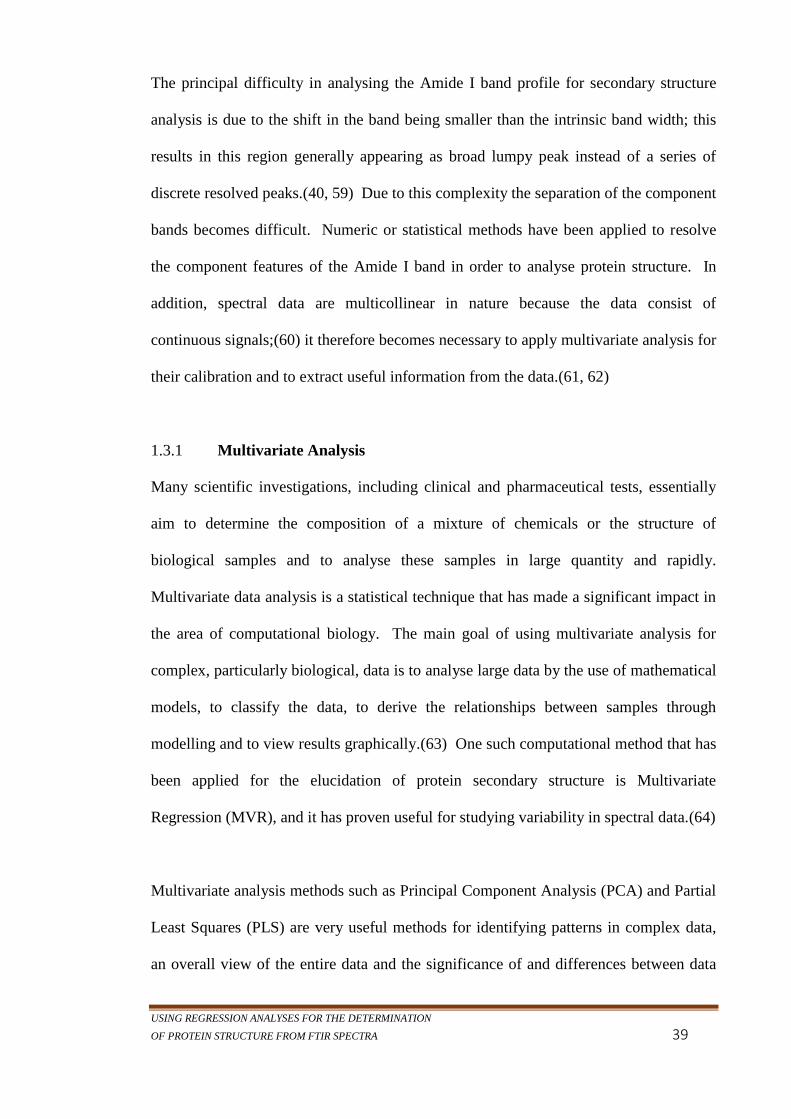
USING REGRESSION ANALYSES FOR THE DETERMINATION
OF PROTEIN STRUCTURE FROM FTIR SPECTRA 39
The principal difficulty in analysing the Amide I band profile for secondary structure
analysis is due to the shift in the band being smaller than the intrinsic band width; this
results in this region generally appearing as broad lumpy peak instead of a series of
discrete resolved peaks.(40, 59) Due to this complexity the separation of the component
bands becomes difficult. Numeric or statistical methods have been applied to resolve
the component features of the Amide I band in order to analyse protein structure. In
addition, spectral data are multicollinear in nature because the data consist of
continuous signals;(60) it therefore becomes necessary to apply multivariate analysis for
their calibration and to extract useful information from the data.(61, 62)
Multivariate Analysis 1.3.1
Many scientific investigations, including clinical and pharmaceutical tests, essentially
aim to determine the composition of a mixture of chemicals or the structure of
biological samples and to analyse these samples in large quantity and rapidly.
Multivariate data analysis is a statistical technique that has made a significant impact in
the area of computational biology. The main goal of using multivariate analysis for
complex, particularly biological, data is to analyse large data by the use of mathematical
models, to classify the data, to derive the relationships between samples through
modelling and to view results graphically.(63) One such computational method that has
been applied for the elucidation of protein secondary structure is Multivariate
Regression (MVR), and it has proven useful for studying variability in spectral data.(64)
Multivariate analysis methods such as Principal Component Analysis (PCA) and Partial
Least Squares (PLS) are very useful methods for identifying patterns in complex data,
an overall view of the entire data and the significance of and differences between data
INTRODUCTION
40
groups by using all relevant variables within the data.(65) The use of PCA in the
biotechnology world has helped in the visualizing and better understanding of the
underlying structure of data or samples in an unsupervised way.(66) PCA has been
used to in the diagnostics of many diseases including the identification and
characterization of biomarkers in cancer cell lines.(67) In food science, PCA has been
used to identify many products including unknown fruits, wines and vegetable oils.(68)
In FTIR spectra of proteins the absorbance of the sample as a function of wavenumber
is affected by chemical and physical properties of the sample as well as being
complicated by overlapping absorption of structural bands.(69) Multivariate analysis
removes the near multicollinearity found in spectral measurements; collinearity
meaning that the different regions of the spectra may convey the same, and therefore
redundant, information. Both Principal Component Analysis (PCA) and Partial Least
Squares (PLS) were developed to solve the near multicollinearity often found in spectral
measurements and the overfitting issues found with predictor (X) variables being larger
than the number of samples;(70)
such a model is said to have a lack of degree of
freedom and thus is over-fitting.(71) PCA (which is explained in the next section) is
considered to be an unsupervised learning method because it does not need a reference
data set for training the model, whereas PLS requires a reference set which spells out
some prior knowledge of the data groupings. The general equation notation of MVR is;
where Y is the matrix of the predicted variable, X is the predictor or observations
variable, β is the determined coefficients during calibration, and ε is the residual error.
Figure 1.7 shows a schematic illustration representing the concepts presented by
equation. 1.3.
Eq. (1.3)
Y = Xβ

USING REGRESSION ANALYSES FOR THE DETERMINATION
OF PROTEIN STRUCTURE FROM FTIR SPECTRA 41
Figure 1.7. Diagrammatic representation of the generalized multivariate equation
represented in eq. 1.3. ‘Y’ is predicted on the basis of ‘X ‘and in such a way that the
residual, ‘ε’ is minimized.
1.3.1.1 Unsupervised learning
There are several unsupervised methods used in the bioinformatics and chemometrics
fields today including PCA, Factor Analysis, and Singular Value Decomposition
(SVD). PCA, which was used in this research, is similar to the mathematical SVD
method except that PCA reduces high dimensional data to a lower dimension in order to
reveal any hidden information in the data. The simplicity and usefulness of PCA has
made it one of the most widely used methods for spectroscopic data analysis; (72-74)
PCA also finds the relationship between observations by finding similar factors (their
correlations) in the observations.(75, 76) The variables of ‘X’ (which are the vectors of
intensities at each wavenumber) are mean centred as explained in section 1.3.2.1; then
the correlations among variables (factors) are computed in the form of a correlation or

INTRODUCTION
42
covariance matrix. The covariance of two variables is their tendency to vary
together.(77) For a sample dataset, this can be written in matrix representation as;
where x is the mean(X), y is the mean(Y), N is the number of entries (observations) in
the dataset. Certain characteristic values referred to as eigenvalues and eigenvectors of
the covariance matrix are calculated as these tell us useful information about the data.
The eigenvectors are variables (intensities at each wavenumber) that form axes in a
multidimensional space; each axis length is determined by scaling the columns of the
data. The eigenvalues are the projected point of each sample on the axis. The
eigenvector (loadings) with the highest eigenvalue (scores) is the most dominant
principle component (PC) of the dataset and these PCs are arranged in order of
importance, that is, PC1 is the component with the largest variation, PC2 is the
components with the second largest variance, and so on. The number of components
that describes close to 100% of the data are extracted based on their significance,
leaving the residual as noise, in this way, PCA is used for dimension reduction.(75)
Each principal component is characterized by the scores ‘T’ (the eigenvalues) and the
loadings ‘P’ (the eigenvectors)(78) so that the product of T*P
T represents the original
data. This notation is given by:
where X is the matrix of spectra of observations, T is the score values, P is the loading
Values, and E contains the residuals also known as noise. In summary, scores are
X = T.PT + E
Eq. (1.4)
N
i
ii
N
yyxxYX
1
))((),cov(
Eq. (1.5)

USING REGRESSION ANALYSES FOR THE DETERMINATION
OF PROTEIN STRUCTURE FROM FTIR SPECTRA 43
linear combinations of the original variables with weights defined by the loadings,
that is, scores are scaled matrix X * P (eigenvector). PCA scores can be plotted to show
the similarities among samples while the loading plot shows similarities in variables
which are the measured intensities at each wavenumber. The class membership of these
objects or samples may not necessarily be known in advance as this may be inferred
during PCA data exploration.(75) Outliers in the PCA do not belong to a known class;
therefore, PCA can detect them during exploration.
1.3.1.2 Supervised Learning
A supervised learning method requires a prior knowledge of the data grouping via a
reference data set. Supervised learning methods include Discriminant Factor Analysis
(DFA) and Multivariate Regression Analysis (MVR).(64) DFA is a supervised
clustering method which determines to what group an individual data belongs. MVR is
used to model the linear relationship between independent variables (the experimentally
observed) and dependent variables (a matrix of FTIR measurements). Input parameters
for most supervised methods are the independent variables (protein spectra) which are
labelled x1...xn, and the dependent variable which is the vector of the fractions of each
secondary structure motif for the proteins.(79) A latent variable, the discriminant
factor, is created from the spectra wavenumbers such as specified in equation 1.6.
where ‘a’ is a constant, ‘b’ is the discriminant coefficients, and ‘x’ is the discrimination
variables. Among the different multivariate calibration methods, Principal Components
Regression (PCR) methods which is based on PCA, and PLS, have received the most
Eq. (1.6)
nn xbxbxbal ...22111

INTRODUCTION
44
attention for the quantitative analysis of spectral data because it is easier to interpret
their models and they work well with small sample size.(70)
PLS (Partial Least Squares)
PLS is a multivariate regression method based on the generalized equation 1.3 where β
is the calculated correlation coefficient and ε is the matrix of experimental noise.(70,
80) In PLS, the value of β is obtained by;
Here, ‘X’ represents the independent measured FTIR spectra and ‘y’ represents the
known secondary structure compositions of the investigated proteins as determined by
X-ray crystallography; ‘X’ is also called a ‘training’ or ‘calibration’ set. PLS regression
is used to predict or determine a new value of ‘y’ from ‘X’ (the FTIR spectral
matrix).(81) PLS modelling captures the variation (or variance) in the spectral matrix in
a low dimensionality model. The total variance of the model is made up of the
Explained Sum of Square (SSE) of the variation of the data, and the unexplained
variance – the residual (SSR).(75) Therefore, the sum of squares of the total variance of
the data set (SST) can be written as: SST = SSE + SSR Eq. (1.8)
The explained variance (also called the goodness of fit) of the data in a model is
calculated as:(75) Explained variance = ((SST – SSR )/ SST)*100
PCR (Principal Component Regression)
The PCR method is based on the basic concept of PCA. PCR performs data
decomposition into the loading and score variables used in building a model. For PCR,
the estimated scores matrix consists of the most dominating principal components of X
Eq. (1.7) yXXX TT 1)(

USING REGRESSION ANALYSES FOR THE DETERMINATION
OF PROTEIN STRUCTURE FROM FTIR SPECTRA 45
and can then be used as input for a regression method. The equation then takes the form
of;
+ εY = XTk
where Y is the predicted response variables, X is the matrix of independent Variables, T
is the matrix of PCA scores and ε is the residual error.(70) As in PCA, these
components are linear combinations of X determined by their ability to account for the
variability in X. The first principal component is computed as the linear combination of
the original X-variables with the highest possible variance; however, unlike PLS, PCR
uses only the X variables for the analysis without employing the ‘y’ variable (the
reference set).
Comparing the two regression methods, PLS regression is known to give good
prediction results with fewer components than PCR because PLS looks for components
that explain the correlation between X and y; the response variable ‘y’ is employed in
the regression. However, the two methods often give comparable prediction results.(61,
70)
Data Pre-processing 1.3.2
Before performing multivariate analyses, data pre-treatment is generally required in
order to reduce the effect of noise, improve the predictive ability of the model and
simplify the model by making the data more normally distributed. Data transformation
is a form of pre-treatment by means of a mathematical formula to change the
distribution of the data, examples of this being logarithmic and exponential
Eq. (1.9)

INTRODUCTION
46
transformation.(61) If the average of each variable is calculated and then subtracted
from the variables, the data are said to be mean-centred. Unit variance scaling means
that the standard deviation (s) for each variable is calculated and by multiplying each
value of that variable by 1/s, all variables are then given an equal weight.(82) This is
also sometimes called variance scaling. These forms of pre-treatments will be
described below.
1.3.2.1 Mean Centring
The reason for centring is to break up the high correlations between each of the main
effect variables and the interaction term, this helps computational accuracy and numeric
stability. (83) Centring converts all the observation points to fluctuations around zero
and not around the mean of the original data. This adjusts for the differences in the
offset between the high and the low numbers.(83) Each variable, Xij, is centred by
subtracting the column mean, Xj, of the data. See eq. 1.10a and eq. 1.10b.
here i is the row index, j is the column index, and x j = column mean.
1.3.2.2 Scaling
In spectroscopic analyses, the difference in the scaling of spectra may arise from the use
of different instruments or scattering effects or path length and other effects.(84, 85) A
scaling approach is useful when the impact of the low wavenumbers needs to be
considered, it is a way to relatively reduce the influence of larger peaks and increase the
Eq. (1.10b)
xxxfjij
)(
n
iijj xx
n 1
1
Eq. (1.10a)

USING REGRESSION ANALYSES FOR THE DETERMINATION
OF PROTEIN STRUCTURE FROM FTIR SPECTRA 47
impact of the smaller spectral features. Small features may be deemed less important in
a multivariate analysis as they do not contribute much to the variance of the data.
Caution should be taken as the inflation of small values, which includes any inflation of
measurement error or instrument misalignment may create an increased danger of
altering the biological meaning of the results.(86, 87) The effectiveness of scaling is
based on data analysis and cannot be predicted in advance.(83) Scaling methods like
normalization, standardization, and multiplicative scattered correction used for
multivariate regression analysis, will be described in this section. Figure 1.8 a-c
illustrates the principles of centred and scaled data.
Figure 1.8a Figure 1.8b Figure 1.8c
Figure 1.8a-c. Figure 1.8a shows the original data points. Figure 1.8b: shows the centred data
which are the individual points minus the mean of the data; this puts the new mean at 0, making
some of the data negative. Figure 1.8c. Scaled data: data looks shortened and broadened in an
attempt to decrease group distance. This results in a zero mean and unit variance of any
descriptor variable.
1.3.2.3 Standardization
Auto-scaling, also known as standardization, is scaling in which each variable is
subtracted from the column mean and divided by its standard deviation; this method
gives the data a standard normal distribution with a zero mean and a unit variance of 1
(the Gaussian distribution).(83) Standardization is performed through;

INTRODUCTION
48
where xij is the variable in j
th Column, x j
is the mean of the column, and S j =
standard deviation of column
1.3.2.4 Normalization
Normalization or range scaling is useful in the identification of biological samples and
for the relationship of the variables in a spectrum as this aids the quantification of the
sample. Range scaling is done by subtracting the spectrum column minimum value
from each column value and dividing by the range of the column (the column maximum
value minus the minimum value), in other words, the length of the data. In this row
operation all sample data are made compatible with each other and spectrum data is
scaled to values between 0 and 1.(88) Range scaling is described in eq. 1.12. Data will
be scaled to a smaller interval if an outlier is present, therefore outliers should be
removed.
where min(xi) is the minimum value for variable xi, max(xi) is the maximum value for
variable xi.
Eq. (1 12)
Eq. (1 11b)
s
xxxf
j
jij)(
1)(0)min()max(
)min()(
xf
xx
xxxf
ii
iij
1
)(1
n
n
ijij
j
xxS
Eq. (1 11a)

USING REGRESSION ANALYSES FOR THE DETERMINATION
OF PROTEIN STRUCTURE FROM FTIR SPECTRA 49
1.3.2.5 Multiplicative Scatter Correction
Multiplicative Scatter Correction (MSC) is another popular scaling method used for the
correction of baselines and for scaling.(89). Multiplicative scatter correction known as
a method in spectroscopy used to correct signals for light scattering and noise or
changes in path length for samples where each sample is estimated relative to that of an
ideal sample.(89) Spectra in a dataset are corrected so that all samples appear to have
the similar scatter level. The correction is done by regressing the measured sample
spectrum against a reference spectrum and then the slope of the fit is used in correcting
the measured protein spectrum.(90) In MSC, as described in eq. 1.13a-b, a reference
spectrum is the mean spectrum of the dataset (r) and the spectrum to be corrected is
defined as (xi). An offset correction like mean-centring is best performed on vector ‘r’
and ‘x’ before the regression.(91-93) For each sample a least squares regression is done
to get an estimate of an unknown factor ‘b’ as shown in eq. 1.13b; this is then used in
the correction of each ith
spectrum in the dataset.
where x = MSC corrected spectrum, Xi = Spectrum in the dataset, b = estimated
unknown factor from eq. 1.13b, and r = the mean spectrum of the dataset.
1.3.2.6 Outliers
There can be unexpected variability in observations, which are called outliers. Outliers
are extremely low or extremely high values in the data set(94) as depicted in Figure 1.9;
Eq. (1.13a)
Eq.( 1.13b)
i
TT xrrrb 1)(
b
xxmsc iˆ)(

INTRODUCTION
50
these outliers are different from the rest of the data due to several reasons; instrumental
errors, or sample error which could be due to incorrect sample labelling or simply a
sample from another data population, or even noise.(92, 93) These factors can have
considerable influence on the calibration. This discrepancy can be eliminated by
removing any outliers after thorough investigation.
0.1 0.2 0.3 0.4 0.5
wavenumber
inte
nsi
ty0
.10
.20
.30
.4
outlier
Figure 1.9. Outlier plot showing a red dot as an outlier, which clearly does not correlate
with the rest of the data.
1.3.2.7 Detection of Outliers
Outliers can be detected by looking at a PCA score plot or looking for a sample residual
with a high number which may mean that the measurement of that sample is erroneous
or less well described by the PCA model. Eq. 1.14a and 1.14b show a simple statistical
formula for detecting an outlier. Firstly, all data points for a given data set are ordered.
The mean of the first half is dedicated as Q1 and the mean of the second half is
dedicated as Q3. The subtraction of Q1 from Q3 gives an Inter-Quantile Range. Any
USING REGRESSION ANALYSES FOR THE DETERMINATION
OF PROTEIN STRUCTURE FROM FTIR SPECTRA 51
data point (xi) larger than Q3 is an outlier, likewise any xi smaller than Q1 is an
outlier.(95)
𝑋 > 𝑄1 + 1.5(𝐼𝑄𝑅)
𝑋 < 𝑄3 + 1.5(𝐼𝑄𝑅)
where: Xi is the data point, Q is a quantile range, IQR is the inter-quantile range. In
multivariate analysis, this is calculated by equation 1.15 which represents the
Mahalanobis Distance which is the square of the distance from the point x to the mean μ
in units of the standard deviation;(96)
where’ x’ is the datapoint, ‘μ’ is the mean of the data and ‘δ’ is the standard deviation.
1.3.2.8 Derivatives
The first and second derivative transformations reduce replicate variability, correct
baseline shift, resolve overlapping peaks, and amplify spectral variations. Broad
overlapping bands of raw spectra become better resolved in a first derivative because it
removes the additive baseline, but it also adds a straight line with a constant slope to the
original spectra;(71) therefore, it is not suitable for obtaining quantitative assignments.
If the first derivative is the slope at each point of the raw spectra, the second derivative
is the slope of the first derivative.(89) The second derivative removes the linear
baseline and thus the ambiguity and complication of assigning the positions of the
features is removed.(97) For this reason, there is an increase in the number of
discriminative features associated with protein spectra and this improve the clarity of
Eq. (1.14b)
Eq. (1.14a)
(x − μ)’δ−1(x − μ) Eq. (1.15)

INTRODUCTION
52
the spectra. Second derivative spectra are commonly used for protein classification;
however, data smoothing should be done first because first and second derivatives
magnify the noise in the spectroscopic data(69). The formulas for the first and second
derivatives are represented in equation 1.16a and 1.16b respectively.
where wy is the measured spectrum at wavenumber w
Validation of the model 1.3.3
Models always have to be validated in order to verify and ensure that they really hold
true in the experimental domain investigated. The validation is needed in order to be
able to decide whether or not the conclusions drawn from it are reliable,(98) i.e. to make
sure that the results can be extrapolated to new data. To estimate the prediction ability
of a model, cross-validation of the data is done by keeping sample or a set of the data
out of the regression analysis and using the model from the analysis to predict the left
out set; this is done for each set of the data which is left out of the regression only once.
The errors from the predictions called Root Mean Square Error for Cross-Validation
(RMSECV) are averaged; (99)(100-102) more information on cross-validation is given
in the Multivariate Calibration Chapter 5. Cross-validation is done to eliminate the
tendency to overfit with too many PLS or PCR components. Number of components
with the lowest RMSECV is always desired and is used to fit the data. It is also good to
know how well a model predicted the data in an independent test set, for this the Root
Mean Squared Error for Prediction (RMSEP) is calculated. To calculate the RMSEP the
individual errors are squared, added together, divided by the number of errors, and then
Eq. (1.16a)
Eq. (1.16b)
1)( ww yyxf
11 2 www yyy

USING REGRESSION ANALYSES FOR THE DETERMINATION
OF PROTEIN STRUCTURE FROM FTIR SPECTRA 53
square rooted. This gives a single number which summarizes the overall error.(103) The
formula for generalized Root Mean Square Error is given in eq. 1.17.
Determination of the unknown 1.3.4
Selection criteria are necessary for the determination of unknown samples as the
training set should have sufficient representation of the group of samples. A large
database is necessary to represent all future samples that may be analysed by the
model.(104)
1.4 Aim of this research
The goal of my research is to develop computational tools that can give better
accuracies for the quantitative analyses and classifications of IR protein spectra to
determine their secondary structures and tertiary folds.
The computational tools developed in this research can contribute to the assessment and
the interpretations of the complexity of protein structures, both in native and denatured
states. The protein structure investigative tools were made by combining machine
learning, multivariate analysis (MVA) methods and Fourier Transformed Infrared
(FTIR); these tools are applicable in real life.
(Eq. 1.17) )ˆ(
1
1
2
i
n
ii
yyn
RMSE
INTRODUCTION
54
Research Objectives 1.4.1
Although the X-ray crystallography technique in determining protein structure is highly
accurate, it is time consuming and not applicable to all proteins; NMR is also limited
by protein size and is not easy to analyse, therefore, complementary methods are
required for proteins where the structure is not easily determined using these techniques.
New methods may also be useful for other purposes, such as to rapidly identify the
critical regions of a spectrum for any given secondary structure motif and to investigate
important structural transitions and processes such as protein folding or aggregation. A
technique, rightly suited for these types of studies is FTIR spectroscopy, the
experimental method chosen for the research presented in this thesis.
Infrared spectroscopy can characterise protein secondary structure conformation;
therefore, it was used in this research to determine the secondary structure of different
motifs in the 84 proteins in H2O solution chosen for this research. FTIR protein
measurements done in-house increased the dataset from its initial count of 28 provided
proteins. The secondary structures of reference proteins from X-ray crystallography
were obtained using Defined Secondary Structure of Proteins (DSSP) script.
To develop a good regression model, the performance of different regression
techniques, PCR, PLS, iPLS, on 84 protein samples, were evaluated; the model with the
optimal performance in terms of predictive results based on the lowest Root Mean
Square Error (RMSE) and Coefficient of Determination (R2) was chosen. To enhance
the predictive ability of each developed model, different data pre-treatment methods, i.e.
cantering, normalization, Standard Normal Variate (SNV), 2nd
derivative and Kennard
Stone data partitioning algorithm, were tested on the ATR-FTIR protein spectra dataset.
They were found to greatly affect the outcome of the data analysis. These methods and

USING REGRESSION ANALYSES FOR THE DETERMINATION
OF PROTEIN STRUCTURE FROM FTIR SPECTRA 55
results with very good accuracies are discussed more in details in each Chapter of this
thesis.
One main objective of this study is to apply a predictive model to estimate the
secondary structure content at each pH of α-lactalbumin. The spectral features of the
denatured protein were evaluated using Principal Component Analysis (PCA) as this
analytical method can be used for data reduction and to explore the data correlation and
understand the biological differences between protein spectra. The most importance
spectral bands were identified using the PCA loadings plot; the identified spectral bands
linked to the discriminating features for each spectrum. Previous spectroscopic studies
have not made an accurate estimation of the secondary structure content of a denatured
α-lactalbumin at each pH level, as has been done in this study.
Secondly, to evaluate the predictive quality of the model, the limit of quantification for
6 proteins (BSA, Ubiquitin, β-lactoglobulin, lysozyme, fibrinogen and IgG) was studied
by analysing the structural content of each protein at the lowest possible concentration.
This study showcases the strength of using FTIR spectra and multivariate analysis for
the detection of low protein concentration in a solution. The results are comparable and
in some cases better than the Circular Dichroism (CD) method which is known to work
well with low protein concentrations.
EXPERIMENTAL METHOD
56
2 Experimental Method: ATR-FTIR spectroscopy
2.1 Introduction
Functional groups present in a molecule tend to absorb IR radiation in the same
wavenumber range regardless of other structures in the molecule, and spectral peaks are
derived from the absorption of bond vibrational energy changes in the IR region.(43)
Thus, there is a correlation between IR band frequencies and chemical structures in the
molecule. In addition to providing qualitative information about functional groups, IR
spectra can provide quantitative information, such as the percentage of the secondary
structure of proteins. For this research, the ATR-FTIR sampling technique was used for
the spectral measurements. The most common sampling techniques used for protein
characterization are transmittance, diffuse reflectance, and attenuated total reflectance
(ATR).(39)
For more explanation on ATR-FTIR techniques, see Chapter 1 – Spectral Analysis.
Analysis of the structural content in the infrared bands, particularly from the Amide I
(1700cm-1
– 1600 cm-1
) and Amide II (1600 cm-1
- 1500 cm-1
) regions will be the main
focus as these have been the most commonly used in the literature for protein studies.
Before any type of analysis was done to elucidate the structure of proteins, data pre-
processing was carried out to eliminate noise, outliers and missing spectral values,
especially in the Amide III region.(105) This section focuses on the collection and
preparation of samples for mathematical evaluations.

USING REGRESSION ANALYSES FOR THE DETERMINATION
OF PROTEIN STRUCTURE FROM FTIR SPECTRA 57
2.2 Sample preparation
Ninety proteins were measured in H2O; 28 of these were supplied by Dr. Parvez Haris
from DeMontfort University (highlighted in light grey in Table A2, Appendix A), and
the rest were collected here at the University of Manchester. Proteins listed in Table A2
in Appendix A were bought from Sigma-Aldrich, and were used without further
purification. Protein samples were prepared at a concentration of 50 mg/ml dissolved in
distilled H2O. Using concentrations at 25 mg/mL or higher provides good precision and
reproducible, quantifiable results;(106) however the study of quantification at lower
protein concentrations down to 0.2mg/ml is discussed in Chapter 5. The pHs of these
samples were recorded and all ATR-FTIR spectra were measured shortly after sample
preparations.
2.3 Spectral measurement and Processing
The ATR accessory, made of a zinc selenide (ZnSe) crystal, was placed into the sample
compartment of a Bruker-Tensor FTIR spectrometer, with an MCT detector being used,
for the spectral measurements. 30 µL of each protein solution was placed on the ATR
cell. A background spectrum of H2O used in the protein preparation was measured for
each protein; this was used as the background signal subtracted from the protein sample
signal for each protein. IR measurements were made with 4cm-1
spectral resolution, 32
scans per sample, over a range from 4000 - 950 cm-1
. Small spectral peaks with
resolution lower than 4 cm-1
tend to disappear and may not be quite suitable for
qualitative examination of spectral components. At higher resolution, the signal to
noise ratio may be low; typically higher resolution (e.g. 1 cm-1
) is used for gas phase
spectra.(35) Acquisition time for each spectrum was less than two minutes for both
background and spectral measurements.
EXPERIMENTAL METHOD
58
Baseline Correction and Atmospheric Correction 2.3.1
The baseline of a measured spectrum should have flat baseline at zero intensity.
Baseline offsets are normally removed by subtracting the value of the minimum
absorbance from the spectrum. This correction was performed for all spectra in the
dataset to remove background absorbance and light scattering effects. Water
subtraction was automatically done by a customized routine in the OPUS 6.2 software
for every spectrum and no smoothing function was applied.
ATR correction 2.3.2
The principles of attenuated total reflection (ATR) have been explained in Chapter 1,
with ATR now being a commonly used sampling technique in FTIR spectroscopy, as
this approach requires minimal sample preparation. However, one of the challenges of
ATR is that its infrared spectra are not identical to that measured in transmission. ATR
spectroscopy introduces some distortion in relative band intensity and absolute shifts to
lower frequency(107). The result of this is higher absorbance bands around the Amide
II region than the Amide I region of a spectrum and this difference between ATR and
transmission spectra may lead to incorrect interpretations. Using the ‘Advance ATR
Correction’ feature on Bruker’s OPUS software, these abnormalities were corrected on
all in-house collected spectra. This distortion can be seen for the fibrinogen spectrum
shown as the blue trace in Figure 2.1a. The Advanced ATR Correction corrected
differences in peak positions and relative intensity ratios of bands in the Amide I and
Amide II regions as seen by the resulting green trace. The new ATR corrected spectrum
should improve the reliability for spectral searches of fibrinogen in spectral libraries.
However, the observation with most spectra in this dataset is that the ratio of Amide I to
Amide II peaks normally maintained by IR transmission spectra was not obtained. This
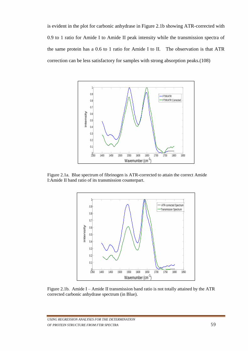
USING REGRESSION ANALYSES FOR THE DETERMINATION
OF PROTEIN STRUCTURE FROM FTIR SPECTRA 59
is evident in the plot for carbonic anhydrase in Figure 2.1b showing ATR-corrected with
0.9 to 1 ratio for Amide I to Amide II peak intensity while the transmission spectra of
the same protein has a 0.6 to 1 ratio for Amide I to II. The observation is that ATR
correction can be less satisfactory for samples with strong absorption peaks.(108)
Figure 2.1a. Blue spectrum of fibrinogen is ATR-corrected to attain the correct Amide
I:Amide II band ratio of its transmission counterpart.
Figure 2.1b. Amide I – Amide II transmission band ratio is not totally attained by the ATR
corrected carbonic anhydrase spectrum (in Blue).
1350 1400 1450 1500 1550 1600 1650 1700 1750 1800 18500
0.1
0.2
0.3
0.4
0.5
0.6
0.7
0.8
0.9
1
Wavemumber (cm-1
)
inte
nsity
FTIR/ATR
FTIR/ATR Corrected
1350 1400 1450 1500 1550 1600 1650 1700 1750 1800 18500
0.1
0.2
0.3
0.4
0.5
0.6
0.7
0.8
0.9
1
Wavemumber (cm-1
)
inte
nsity
ATR-corrected Spectrum
Transmission Spectrum
EXPERIMENTAL METHOD
60
2.4 Data Pre-processing for Multivariate Analysis
The proteins’ secondary structural motif fractions were obtained using Defined
Secondary Structure of Proteins (DSSP)(109) script. The Protein data bank (PDB) does
not give the percentage of secondary structure assignments beyond α-helix, β-sheet and
other; however the PDB file for each protein contains the structural information which
can be fed into the DSSP script. The DSSP code assigns eight secondary structures of
which six are popularly used in protein prediction namely, α-helix, β-sheet, π-helix, 310-
helix, turns, and coils (other); denoted by (H), (E), (I), (G), (T), (“ “).(110) A perl script
was developed in-house to extract these structural compositions from PDB files using
the DSSP script and all spectra pre-processing steps were performed using Matlab
versions R2010 and R2013. Of the six secondary structure assignments, π-helix was not
considered for this project because it is a rare protein secondary structure element;
however, β-sheet structure was further split into parallel and antiparallel β-sheets. See
Appendix A, Table A2 for the 90 proteins and their secondary structure fractions as
derived from DSSP script. Data pre-processing was done on all collected protein spectra
to identify or remove outliers, checking for inconsistencies and missing values and
normalizing the intensities of the data. Figure 2.2 shows the raw spectra of the 90
protein samples.
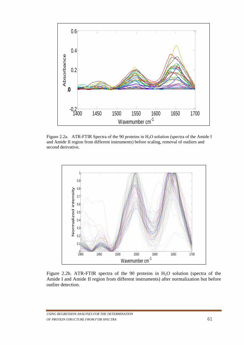
USING REGRESSION ANALYSES FOR THE DETERMINATION
OF PROTEIN STRUCTURE FROM FTIR SPECTRA 61
Figure 2.2a. ATR-FTIR Spectra of the 90 proteins in H2O solution (spectra of the Amide I
and Amide II region from different instruments) before scaling, removal of outliers and
second derivative.
Figure 2.2b. ATR-FTIR spectra of the 90 proteins in H2O solution (spectra of the
Amide I and Amide II region from different instruments) after normalization but before
outlier detection.
1400 1450 1500 1550 1600 1650 1700-0.2
0 .0
0.2
0.4
0.6
Wavemumber cm-1
Absorbance
1400 1450 1500 1550 1600 1650 17000
0.1
0.2
0.3
0.4
0.5
0.6
0.7
0.8
0.9
1
Wavemumber cm-1
Norm
alized inte
nsity

EXPERIMENTAL METHOD
62
Outlier Detection 2.4.1
For proteins in H2O, the Amide III region often had missing data, therefore only the
Amide I and II regions of the spectra were used; these spectra with missing values were
the 28 protein spectra not collected in house (mentioned in section 2.2). Samples with
the Amide III region were used for some experiments that required the study of fewer
proteins; e.g., the study of protein denaturation as seen in Chapter 5. Spectra that were
too noisy to resolve were also removed from the dataset. The removal of unusable
spectra reduced the database size from 90 to 84. These six spectra are: amyloglucanase,
galactose oxidase, d-glucosamin, isocitric dehydrogenase, spectrin, and theamalysin.
Statistical methods for multivariate outliers indicate those observations far from the
centre of the data distribution as outliers.(93) Mahalanobis distance was used for the
calculation of outliers and this is described in section 1.3.2.4 (Detection of Outliers) of
Chapter 1, but it is basically involves a measure of the square of the distance of each
spectrum to the mean of the spectra. Any distance outside the calculated radius,(93, 94)
as given by equation 1.4, is an outlier. These steps are listed below:
1. Spectral matrix: An n × d data set, S.
2. Calculate the mean (μ) and variance-covariance (Σ) of the matrix.
3. Let M be n × 1 vector consisting of square of the Mahalanobis distance to μ.
Where n is the number of samples in the dataset and M is the Mahalanobis
distance, equal to (x − μ)’ Σ -1
(x − μ)
4. Find points ‘p’ in M whose value is greater than the significance level
[𝑖𝑛𝑣(√𝑥𝑑2(.975)) ] : χ
2 (chi square) distribution with ‘d’ degrees of freedom.
5. Return ‘p’ (This is the outlier with value greater than the significant level)

USING REGRESSION ANALYSES FOR THE DETERMINATION
OF PROTEIN STRUCTURE FROM FTIR SPECTRA 63
The plot of the mean and standard deviation of each sample in Figure 2.3a shows that
protein number 88 (d-glucosamine) and protein number 22 (spectrin) are above the
significant level. D-glucosamine differs from the rest of the proteins because it is a
sugar and not a protein and belonged to a different dataset. The spectrin sample could
have been affected during measurement, if left in the dataset it shows as an outlier and
affects the results of the spectral analysis and so was taken out of the 29 samples sent
from Dr. Parvez Haris of DeMontfort University. An evaluation of their mean
prediction errors shows them to be higher than normal and they were therefore treated
as being unreliable. These samples were removed as shown in Figure 2.3b.
Figure 2.3a. Outlier detection using mahalanobis distance. Plot shows D-glucosamine
(sugar) and Spectrin as outliers. The mean of each spectrum and the standard deviation of
each sample are plotted on the x-axis and y-axis, respectively

EXPERIMENTAL METHOD
64
Figure 2.3b. Distribution of protein samples after outliers were taken out.
Centring and Scaling. 2.4.2
Intensities of the 84 protein spectra measured in H2O were scaled to prevent spectra
with strong peaks from obscuring spectra of smaller bands with equally significant
spectral features.(84) The dataset is divided into Amide I, and II, each region was
selectively scaled separately to ensure the significance of each contributing spectrum.
Normalization or range scaling used for this dataset is useful in the identification of
biological samples and for the relationship of the variables in a spectrum as this aids in
the quantification of the sample.(88). Range scaling is done by subtracting the spectrum
column minimum value from each column value and dividing by the range of the
column (the column maximum value minus the minimum value); see section 1.3.2 in
chapter 1 for more information on scaling. In this row operation all sample data are
made compatible with each other and spectral data are scaled to values between 0 and
1.(88) Standardization, which is a column operation also used for scaling, was
performed on the dataset for comparison purposes. Chapter 1, section 1.3 gives the

USING REGRESSION ANALYSES FOR THE DETERMINATION
OF PROTEIN STRUCTURE FROM FTIR SPECTRA 65
formulae for normalization and standardization. Standardization is useful when the
precise number of biological components varies but the relative proportions of the
sample structure, as in the percentage of their secondary structure compositions, can be
measured quantitatively(111). In the methods below, both normalization, and Standard
Normal Variate (SNV), were first performed separately and then together to evaluate
their effect. The scaled data are shown in Figure 2.4.
Figure 2.4. 84 scaled protein spectra (Amide I region) measured in H2O
Multiplicative Scattered Correction (MSC) 2.4.3
Both the original and scaled data were further pre-treated with MSC as described in
section 1.3 of Chapter 1. MSC is a relatively simple processing step that attempts to
account for scaling effects and offset (baseline) effects(112). This method should
correct the multiplicative effect on all other samples to the level of the mean sample.
Judging from the plots below (Figure 2.5a and 2.5b) it may be easy to conclude that
1600 1610 1620 1630 1640 1650 1660 1670 1680 1690 17000
0.1
0.2
0.3
0.4
0.5
0.6
0.7
0.8
0.9
1
inte
nsity
Wavemumber (cm-1
)

EXPERIMENTAL METHOD
66
multiplicative scatter correction was effective because the spectra are tightly grouped
with better separated peaks than that of the Figure 2.4, but this will only be confirmed if
regression analyses on this data give lower prediction errors.
Figure 2.5a. MSC pre-processing performed on 84 raw data showing reduction in spectral
intensities. Spectra are pulled towards the raw spectrum with the mean value
Figure 2.5b. MSC pre-processing performed on normalized spectra. Spectra are pulled
towards the normalized mean sample.
1600 1610 1620 1630 1640 1650 1660 1670 1680 1690 1700-0.1
-0.05
0
0.05
0.1
0.15
0.2
0.25in
tensity
Wavemumber (cm-1
)
1600 1610 1620 1630 1640 1650 1660 1670 1680 1690 1700-0.4
-0.2
0
0.2
0.4
0.6
0.8
1
1.2
1.4
inte
nsity
Wavemumber (cm-1
)

USING REGRESSION ANALYSES FOR THE DETERMINATION
OF PROTEIN STRUCTURE FROM FTIR SPECTRA 67
Standard Normal Variate (SNV) 2.4.4
Figures 2.6a and 2.6b below show the result of SNV on the protein samples measured in
H2O, by subtracting the mean of the data from each value and dividing by their standard
deviation, which gives each sample a unit deviation of 1. Judging from the intensity of
the plots, it appears that SNV scaling gave a much tighter grouping of the data when
they were normalized than without normalization; however, Table 2.1 shows the
minimum and maximum intensities of the spectra after scaling with each of these
methods. SNV and MSC plots look very similar in their peak separation and clustering;
their similarity will be compared in Chapter 4 for regression analysis.
Figure 2.6a. SNV pre-processing performed on 84 protein spectra of raw protein samples
1600 1610 1620 1630 1640 1650 1660 1670 1680 1690 1700-2.5
-2
-1.5
-1
-0.5
0
0.5
1
1.5
2
2.5
inte
nsity
Wavemumber (cm-1
)

EXPERIMENTAL METHOD
68
Figure 2.6b. SNV pre-processing done on normalized 84 protein spectra
2nd Derivative 2.4.5
Since spectra were recorded on different days and in different labs, which are factors
known to affect spectral response, another way to correct instrumentation errors that
was investigated was to calculate the second derivative of all spectra to compare results
to the results of normalization and standardization. With FTIR data it is not uncommon
to differentiate spectra to the 1st or 2
nd derivative as it improves the separation of non-
resolved peaks.(113) Second derivative analyses were employed to reduce any scatter
effects and to extract any latent spectroscopic information that may be hidden in the
broadened background. Matlab software provides a derivative function which was used
to determine 2nd
derivatives. The plots in Figure 3.7 show the 2nd
derivatives of the
normalized 84 proteins samples in H2O.
1600 1610 1620 1630 1640 1650 1660 1670 1680 1690 1700-2
-1.5
-1
-0.5
0
0.5
1
1.5
2
2.5
inte
nsity
Wavemumber (cm-1
)

USING REGRESSION ANALYSES FOR THE DETERMINATION
OF PROTEIN STRUCTURE FROM FTIR SPECTRA 69
Figure 2.7. Second derivative on the normalized data of the ATR-FTIR spectra of 84
proteins collected in H2O
.Table 2.1. A table of pre-processing methods and their minimum and maximum values of
spectral intensities.
Pre-processing Method Min Value Max Value
Normalization 0 1
MSC on Raw Spectra -0.0743 0.2645
MSC on Normalized Spectra -0.1956 1.4587
SNV on Raw Spectra -2.3510 2.1815
SNV on Normalized Spectra -1.7878 2.2367
2nd
Derivative -0.0471 0.0494
1620 1630 1640 1650 1660 1670 1680 1690 1700-0.1
-0.05
0
0.05
0.1
d2A
/dv
2
Wavenumber (cm-1
)

EXPERIMENTAL METHOD
70
2.5 Discussions
Although it is common for pre-processing methods to be used before multivariate
modelling, there is no set standard approach and the results of multivariate analysis are
affected by the methods used. This also means that data pre-processing is often revisited
to ascertain optimal solutions before performing any computational analysis.
The ATR-FTIR technique is highly popular, but it introduces some spectral distortions
that are problematic when comparing spectra of ATR and transmission(114, 115). The
ATR correction does improve the similarity between the transmission and ATR spectra,
but the correction is far from perfect. Corrected ATR-FTIR spectra will be used for
both quantitative and qualitative analysis in this project for compatibility purposes.
One common method of pre-processing used on spectroscopic data is normalization
which involves setting each observation (spectrum) to have unit total intensity by
expressing each data point as a fraction of the total spectral integral. This is referred to
as normalization to a constant sum.(88) Normalization helps in reducing the variations
in data from different scaling and makes apparent the peak intensities that are the
discriminating features. Standardization, which is also commonly used, is performed on
the columns of spectral intensities across all samples, giving each column of the data a
zero mean and a standard deviation of 1. The weighting of standardization reflects the
data correlation and is performed so that Multivariate Analysis, such as Principal
Component Analysis (PCA) and Partial Least Squares (PLS), components have the
centre of the data as their origin, which results in the use of a minimal number of
components in a model.(116)

USING REGRESSION ANALYSES FOR THE DETERMINATION
OF PROTEIN STRUCTURE FROM FTIR SPECTRA 71
From the above plots, MSC operations on the original dataset tightened and reduced the
intensities of the data while SNV centred the data (to give a covariance) and scaled at
the same time to give a correlation of the samples in the dataset. Comparing the SNV
plots in Figure 2.6 a/b to the plot of the normalized spectra in Figure 2. it is obvious that
SNV gives tighter groupings of the measurements and a better attempt at peak
separation. In fact, SNV has been shown to do better with infrared spectroscopic data of
this sort;(65) however, the normalized plot keep the spectra as close to its original form.
Again, comparison of the modelling results from these methods will decide on what pre-
processing method(s) to use.
Pre-processing methods employed by an analyst would depend on the intended purpose,
for example, the biological information to be extracted, or looking for the variations in
the data.(116) Whereas different analysts use one method or another, a combination of
the two methods may be useful for data pre-processing to correct multiplicative scatter
effects and aid in the extraction of important features through multivariate analysis.
Normalization also allows for the identification of biological samples and for the
analysis of the most contributing factors for the variations in the data. This can be done
by plotting and studying the loadings of PCA which is done in the next chapter. Due to
the use of PCA to study structural variations in protein, normalization may be used for
in Chapter 3 unless SNV or MSC give better results. The use of 2nd
derivative helps in
resolving the underlying peaks of the spectra to aid in the quantification of the data, so
this method will be used. Not only does normalization help with biological
identification of samples, the relationship of the variables in the spectra can also be
extracted whereby helping with quantification of the data. As can be seen by Figure
2.4, normalization (range scaling) also keeps the data close to their original form as

EXPERIMENTAL METHOD
72
opposed to SNV and MSC but SNV and MSC centred the data better than
Normalization. The data had already been baseline corrected which MSC and SNV are
good for; however, these three methods will be tested in Chapter 4 which deals with
quantitative analysis as performance of pre-processing method is not easy to analyse
prior to modelling.(91)

USING REGRESSION ANALYSES FOR THE DETERMINATION
OF PROTEIN STRUCTURE FROM FTIR SPECTRA 73
3 PCA Protein Structure Classification
3.1 Introduction
Fourier Transform Infrared (FTIR) spectral data are multivariate (covering hundreds of
wavenumbers), and collinear,(69, 86) meaning that every data point in a protein
spectrum is highly influenced by the next data point due to overlapping absorption
bands of biomolecules caused by spectral shift. (117, 118) In addition to the spectra of
protein samples being heavily influenced by the covariance between biological
components, the differences between FTIR spectra are often subtle making it potentially
difficult to distinguish proteins from each another, particularly when they have similar
structures. To be able to extract meaningful information from these spectra,
multivariate analysis can be applied to correctly classify the spectra based on the
differences in their structural content (119) and also to identify the spectral features that
contribute the most to the spectral differentiation.(120, 121) The usefulness of the
identification of protein structural features and their FTIR marker bands is in the
determination of the structure and the quality (aggregation, degradation, impurities, etc.)
of the protein samples, and also for the identification of unknown samples.
This main aim of this chapter is to explore the existing protein classes in terms of their
secondary structure groups and tertiary folds using spectra measured with ATR-FTIR
spectroscopy (spectral measurements and pre-processing are explain in Chapter 2) and
to create a model with which to qualitatively analyse protein samples to determine their
structures, and this is made possible by applying Principal Component Analysis (PCA).

PROTEIN STRUCTURE CLASSIFICATION
74
The two widely used protein classification systems are CATH(17) (Class, Architecture,
Topology, Homologous superfamily) and SCOP(18) (Structural Classification of
Proteins) and the protein classification assignment used by both systems is based mainly
on X-ray crystallographic measurements. CATH divides proteins into 4 classes (mainly
α, mainly β, αβ, and few secondary structures), while SCOP divides them into 11
protein classes of which 10 were covered by the protein selection in this dataset. These
classes are: All α, All β, α/β, α+β, multi domain (αβ), membrane and cell surface, Small,
Coiled-coil, Peptides, and Designed Proteins. Low resolution is the 11th
class type but it
is not covered in this study simply because there was not any protein of this class
investigated in-house. In this chapter, the PCA results for each protein in our dataset
were compared to those of SCOP, the gold standard for structure comparison, to
determine their class distributions based on their FTIR spectra. SCOP also has the
domain definitions used in this research for protein structure identification.
The PCA method has been previously described in Section 1.3.1 as a multivariate
statistical technique used to reduce data dimensions and to objectively explore the
data.(67) The fewer variables in the FTIR data after reduction of redundant information
make it easier for the data to be explored graphically and statistically; PCA eliminates
data that are not useful in differentiating the protein FTIR spectra, and classifies them as
noise.(68, 122) We have used pre-processing methods, particularly normalization, as
described in Section 2 to remove some linear correlations in the data before PCA
classification of the FTIR dataset. Without normalization of the spectra, the most
intense spectral bands become dominant.(91, 123, 124)
PCA was applied to the Amide I and Amide II regions of ATR-FTIR protein spectra
measured in H2O to perform data reduction, and also to look for variations in the data

USING REGRESSION ANALYSES FOR THE DETERMINATION
OF PROTEIN STRUCTURE FROM FTIR SPECTRA 75
and to group the spectra according to their similarities or differences in structure which
can be viewed by the observation and analysis of the plots of principal component
scores and loadings;(125) therefore, protein structures were identified based on the
similarity of the principal component scores of their IR spectra.
3.2 Dataset used for this method
The Amide I region used for this analysis has a total of 101 data points for each
spectrum, in the range of 1700 cm-1
to 1600 cm-1
spaced 1 cm-1
apart. The measured
ATR-FTIR spectra were put into a matrix form; each row of the matrix corresponds to a
spectrum. and each column is the absorbance at a different wavenumber.(126) The
Amide II region from 1600 cm-1
to 1480 cm-1
contains 121 data points; in all, there are
84 protein spectra in this dataset which are listed in Table A2 in Appendix A. The
dataset is summarized below:
Amide I region: 84x101 matrix of soluble Protein Spectra Data in H2O
Amide II region: 84x121 matrix of soluble Protein Spectra Data in H2O
3.3 PCA Model
Sample preparation and ATR-FTIR spectral collection for this study are described in
Sections 2.2 and 2.3. Data points in the ATR-FTIR spectra, as described in Chapter 2,
were first normalized and autoscaled using the Standard Normal Variate (SNV)
approach. This scaling technique takes care of centring each spectrum by subtracting
the mean value of the spectrum from each spectrum value and this gives the spectrum a
new mean of 0; SNV then scales each spectrum by its standard deviation which gives

PROTEIN STRUCTURE CLASSIFICATION
76
the spectrum a variance of 1; this process is described under ‘Data Processing’ in
Section 1.3.2.2 and Section 2.4.2.
Bands in the Amide I region mostly originate from C=O stretching vibrations and those
in the Amide II region originate mostly from NH bending vibrations. PCA is a pattern
recognition method which does not require a priori knowledge about the protein
structure, and was applied to data for the Amide I and Amide II regions for the 84
proteins in the dataset in order to decompose the FTIR data matrix (X) into scores (T),
and loadings (P). Columns of ‘P’ are values of the calculated covariance (XTX) of ‘X’
and are called the eigenvectors which are the new coordinate axes.(127) The scores,
‘T’, are the new values of the protein samples projected onto each eigenvector. The
principal components (PCs) are the arrangements of eigenvectors according to the
number of variance (non-zero eigenvalues). The sum of the vectors, TPT, represents the
ATR-FTIR data matrix, X. The PCs produced by PCA are ordered by importance to the
data; that is, PC1 has the highest amount of variation, followed by PC2, etc.(126, 128,
129) Principal Component Analysis is covered in the introduction under ‘Multivariate
Analysis’ (Section 1.3.1).
The result of the data decomposition into scores and loadings by PCA is returned in a
matrix of normalized eigenvectors stored in columns (as numbers of loadings ‘P’), and
eigenvalues of each sample (scores ‘T’) stored in rows. The loadings of the principal
components highlight relevant information within the spectra for differentiation. Again,
loadings with no significance are excluded as noise. The first PC, (t1, p1T), gives the
maximum variation in the protein samples, the second principal component is
orthogonal to the first, and describes the maximum of the variation not described by the

USING REGRESSION ANALYSES FOR THE DETERMINATION
OF PROTEIN STRUCTURE FROM FTIR SPECTRA 77
first PC, and so on.(127, 130, 131) Each of these components can be expressed in
terms of their original variables as:
pp xbxbxby ...22111
where: y represents the principal components, b represents the calculated coefficients,
x represents columns of the original measured data and p represents the number of
dimensions.(132) The number of PCs that describe the variations in the protein dataset,
with PC1 being the highest, were selected through a PC plot vs. percentage of the
variance explained. In this analysis, the PCs that gave the highest variance in the data
were considered for the study of the secondary structure information of the 84 measured
proteins. These chosen numbers of PCs were also used in plotting the scores and
loadings for the inspection of peaks influential in distinguishing the protein spectra.
The scattered plots of the PC scores are correlated with the loading plot of the same
dataset to view the influence of spectral wavenumbers on the dataset groupings.
3.4 Model Validation
An unsupervised learning method like PCA does not have a reference dataset, as is
found in supervised learning (133). To validate findings from PCA, the dataset can be
split in two before PCA and their results compared for similar samples and groups. If
the scores and the loadings for the two halves are comparable, then the model is valid.
However, in our case, there are also the SCOP structural assignments of these proteins
which can be used to validate results.
Eq. (3.1)
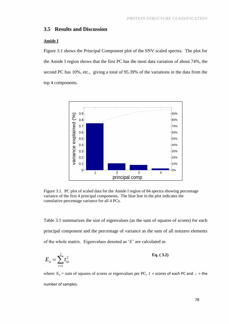
PROTEIN STRUCTURE CLASSIFICATION
78
3.5 Results and Discussion
Amide I
Figure 3.1 shows the Principal Component plot of the SNV scaled spectra. The plot for
the Amide I region shows that the first PC has the most data variation of about 74%, the
second PC has 10%, etc., giving a total of 95.39% of the variations in the data from the
top 4 components.
Figure 3.1. PC plot of scaled data for the Amide I region of 84 spectra showing percentage
variance of the first 4 principal components. The blue line in the plot indicates the
cumulative percentage variance for all 4 PCs.
Table 3.1 summarizes the size of eigenvalues (as the sum of squares of scores) for each
principal component and the percentage of variance as the sum of all nonzero elements
of the whole matrix. Eigenvalues denoted as ‘E’ are calculated as
where: Ea = sum of squares of scores or eigenvalues per PC, t = scores of each PC and j = the
number of samples.
1 2 3 40
0.1
0.2
0.3
0.4
0.5
0.6
0.7
0.8
0.9
principal comp
va
ria
nce
exp
lain
ed
(%
)
0%
10%
20%
30%
40%
50%
60%
70%
80%
90%
Eq. ( 3.2)
j
i
iaa tE1
2

USING REGRESSION ANALYSES FOR THE DETERMINATION
OF PROTEIN STRUCTURE FROM FTIR SPECTRA 79
Table 3.1. PCA analysis for the Amide I region listing the eigenvalues Sum of Squares,
their percentage variance and the cumulative variance.
Amide I Region
PC E %Vi Cumulative %V
1 7.56 74.32 74.32
2 1.07 10.50 84.82
3 0.82 8.05 92.87
4 0.26 2.52 95.39
5 0.15 1.49 96.89
6 0.11 1.07 97.96
7 0.05 0.44 98.41
8 0.03 0.34 98.74
9 0.03 0.32 99.06
10 0.02 0.23 99.29
PC= number of Principal Component
E = eigenvalues
%Vi = eigenvalues presented as percentage
Cumulative %V = accumulated percentage of V
As mentioned above, a score is the amount of latent variable for a particular sample
(protein). Each sample has a score value for every principal component. Proteins
grouped together are similar in properties, so analysis of the loading plot helped to
identify the discriminatory wavenumbers for the structural bands of the protein spectra.
Figure 3.2 shows the Amide I data projection onto the first two principal components.
PC1 separates the proteins’ spectral bands in the Amide I region into α-helices on the
left and β-sheets on the right.

PROTEIN STRUCTURE CLASSIFICATION
80
Fig
ure
3.2
. P
CA
sco
res
plo
t fo
r A
mid
e I
regio
n (
1600 c
m-1
– 1
700cm
-1)
of
AT
R-F
TIR
sp
ectr
a of
84
pro
tein
s in
H2O
(P
C1
xP
C2
).
Plo
t sh
ow
s th
e cl
ust
erin
g o
f sc
ore
s.
Blu
e dots
are
pri
mar
ily α
pro
tein
s, r
ed d
ots
are
pri
mar
ily
β p
rote
ins,
gre
en d
ots
in
dic
ate
pro
tein
s o
f o
ther
types
-10
-8-6
-4-2
02
46
810
-3-2-10123
Firs
t Prin
cipa
l Com
pone
nt
Second Principal Component
alph
a ca
sein
d amin
o ac
id d
ehyd
rco
llage
n
avid
in conc
anav
alin
porin
chym
otry
psin
apha
-cry
stal
linIg
G (
bovi
ne)
IgG
(hu
man
)ca
rbon
ic a
nhyd
rase
alph
a am
ylas
e-ty
pe2
tryp
sin(
hog)
tryp
sin
ribnu
S
typs
in-c
hym
oin
vert
ase
lect
in
Pro
tein
ase
-la
ctog
lobu
lin
elas
tin
peps
inal
pha-
1-an
titry
psin
lglu
tath
ion
lact
ic d
ehyd
rog
l-lac
tic
gluc
ose
oxid
ase
stap
hylo
kina
se-B
es
tera
se(b
.sub
stilis
)
insu
lin
myo
glob
in
tran
sket
alos
e
ferr
itin
albu
min
(bo
vine
)
albu
min
(hu
man
)
alph
a lacto
glph
tosy
stem
II
cyto
chro
me
mel
ittin
rhod
opsi
n bl
each
ed
calm
odul
in
pig
citr
ate
synt
hase
anne
xinV
purp
le m
embr
ane
tryp
toph
an
subt
ilisin
phos
vitin
urea
sees
tera
se(R
.ory
zae)
apro
tinin
pa
pain
lipas
e(C
.rug
osa)
nativ
e-an
ti-th
rom
bin
sp
lit-o
valb
umin
nt-o
valb
umin
othe
r

USING REGRESSION ANALYSES FOR THE DETERMINATION
OF PROTEIN STRUCTURE FROM FTIR SPECTRA 81
Figure 3.3. Loading Plot of the Amide I (1600 cm-1
– 1700cm-1
) region for spectra of 84
proteins in H2O This Plot shows the clustering of scores. Wavenumbers of spectral signals
indicate the discriminating features associated with clustering of scores in Figure 3.2.
Figure 3.4. PC1, PC2, and PC3 loadings plot of Amide I (1600 cm-1 – 1700cm-1) region for spectra of 84 proteins in H2O (PC1xPC2). The wavenumbers listed indicate the discriminating features associated with clustering of scores in Figure 3.2. Both Figure 3.3 and Figure 3.4 were combined in the analysis of the scores plot (Figure 3.2).
-0.2 -0.15 -0.1 -0.05 0 0.05 0.1 0.15 0.2-0.25
-0.2
-0.15
-0.1
-0.05
0
0.05
0.1
0.15
0.2
0.25
Loading for PC1
Load
ing
for
PC
2
1630
1660
1657
1658
1659
1652
1674
1692
1700 1644
1635
1610
1600 1620 1640 1660 1680 1700-0.2
-0.15
-0.1
-0.05
0
0.05
0.1
0.15
0.2
0.25
Wavenumber (cm-1
)
Inte
nsity
1642
1630
1635
16221609
16521657
1662
1674
1688
1693
Loading for PC1
Loading for PC2
Loading for PC3
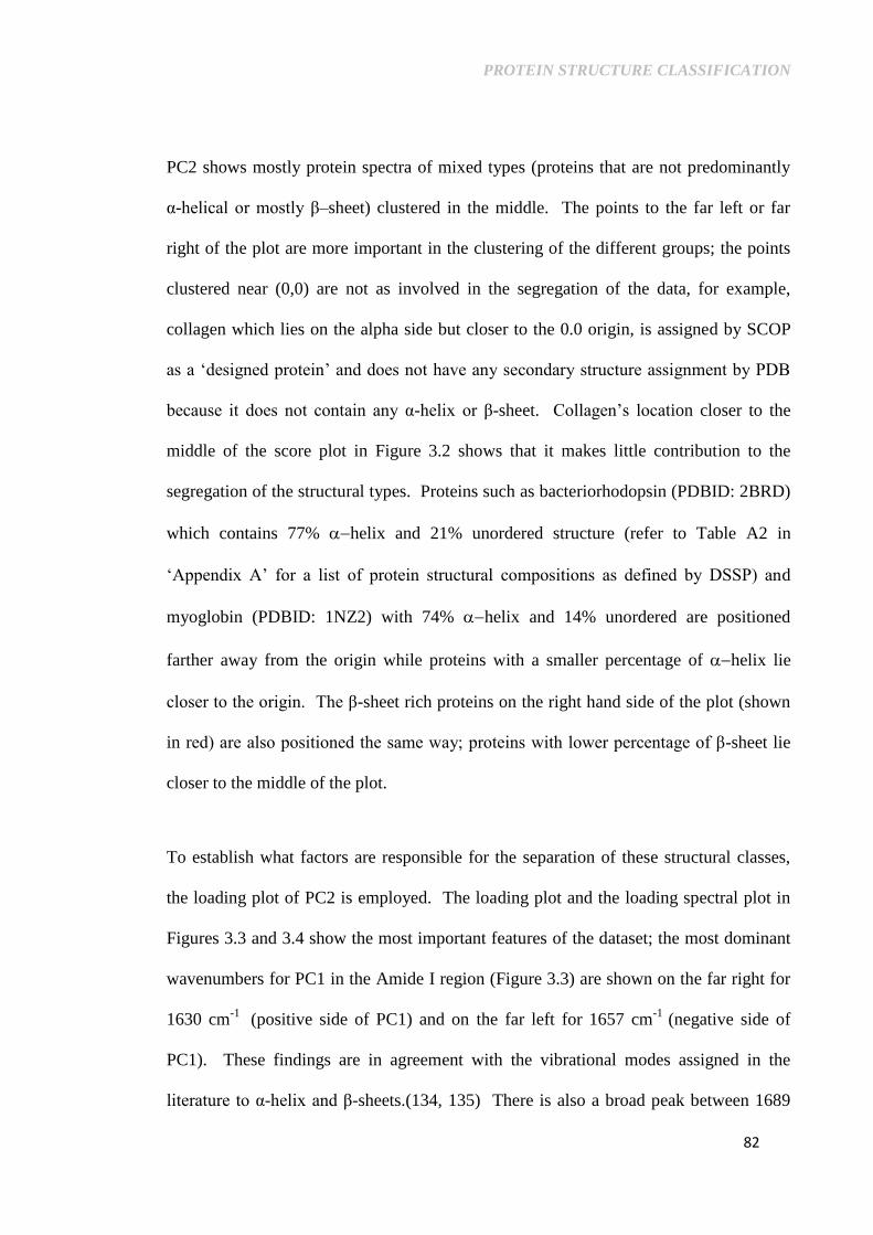
PROTEIN STRUCTURE CLASSIFICATION
82
PC2 shows mostly protein spectra of mixed types (proteins that are not predominantly
α-helical or mostly β–sheet) clustered in the middle. The points to the far left or far
right of the plot are more important in the clustering of the different groups; the points
clustered near (0,0) are not as involved in the segregation of the data, for example,
collagen which lies on the alpha side but closer to the 0.0 origin, is assigned by SCOP
as a ‘designed protein’ and does not have any secondary structure assignment by PDB
because it does not contain any α-helix or β-sheet. Collagen’s location closer to the
middle of the score plot in Figure 3.2 shows that it makes little contribution to the
segregation of the structural types. Proteins such as bacteriorhodopsin (PDBID: 2BRD)
which contains 77% helix and 21% unordered structure (refer to Table A2 in
‘Appendix A’ for a list of protein structural compositions as defined by DSSP) and
myoglobin (PDBID: 1NZ2) with 74% helix and 14% unordered are positioned
farther away from the origin while proteins with a smaller percentage of helix lie
closer to the origin. The β-sheet rich proteins on the right hand side of the plot (shown
in red) are also positioned the same way; proteins with lower percentage of β-sheet lie
closer to the middle of the plot.
To establish what factors are responsible for the separation of these structural classes,
the loading plot of PC2 is employed. The loading plot and the loading spectral plot in
Figures 3.3 and 3.4 show the most important features of the dataset; the most dominant
wavenumbers for PC1 in the Amide I region (Figure 3.3) are shown on the far right for
1630 cm-1
(positive side of PC1) and on the far left for 1657 cm-1
(negative side of
PC1). These findings are in agreement with the vibrational modes assigned in the
literature to α-helix and β-sheets.(134, 135) There is also a broad peak between 1689

USING REGRESSION ANALYSES FOR THE DETERMINATION
OF PROTEIN STRUCTURE FROM FTIR SPECTRA 83
and 1697 cm-1
; which may indicate anti-parallel β-sheet as this has been reported in the
literature as registering between these frequencies.(136) The factors are arranged so
that when one factor is high for an observation, the other factor is low for the same
observation (135), therefore scores with more α-helical structure would lie opposite to
those scores with more β-sheet structure. The principal components distinguish between
observations that have high and low frequency value contributions (numbers above and
below zero). The results reported here are in good agreement with literature
assignments for the FTIR bands for both α-helix and β-sheets.(50)
As mentioned earlier, the score plot (Figure 3.2) shows that PC2 highlights proteins
with approximately equal amounts of α-helix and β-sheet closer to the origin and those
with more α-helix or more β-sheet farther away. A loading spectra plot is an alternative
way of identifying the most significant peaks, which may not be readily visible from
just the loading plot alone. PC2 on the loading spectra plot shows a pronounced peak at
1635 cm-1
(in agreement with the spectrum of PC1 in that region for β-sheets) and
around 1672 - 1675 cm-1
, which is mainly associated with β-turns.(50, 117) PC2 also
detected a band near 1653 cm-1
on the farthest negative side of the plot. Scores of PC2
were investigated further as shown in Figure 4.5.
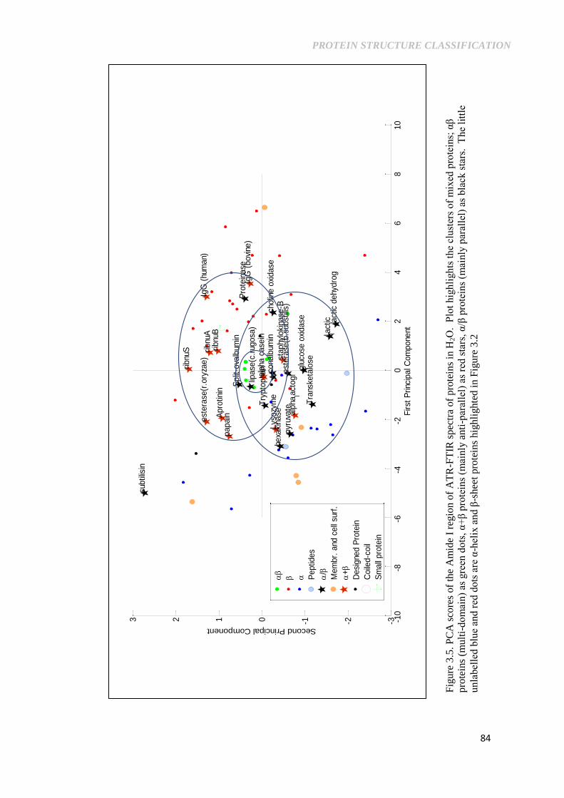
PROTEIN STRUCTURE CLASSIFICATION
84
-10
-8-6
-4-2
02
46
810
-3-2-10123
First
Princ
ipal C
om
pone
nt
Second Principal Component
IgG
(hu
man)
ribnu
S ribnu
Aribnu
B
IgG
(bovi
ne)
Pro
tein
ase
cholin
e o
xidase
lact
ic d
ehy
dro
gl la
ctic
glu
cose
oxi
dase
Tra
nske
talo
se
alp
hala
ctogl
staphy
loki
nase
-B
est
era
se(b
.sub
stili
s)
cona
lbum
in
pyr
uvate
Lys
ozy
me
hexa
kina
se
Try
pto
pha
nalp
ha c
ase
in
Split
-ova
lbum
in
lipase
(c.r
ugosa
)
Apro
tinin
est
era
se(r
.ory
zae)
papain
subtil
isin
Peptid
es
/
Mem
br.
and
cell
surf
.
+
Desi
gne
d P
rote
in
Coile
d-c
oil
Sm
all
pro
tein
Fig
ure
3.5
. P
CA
sco
res
of
the
Am
ide
I re
gio
n o
f A
TR
-FT
IR s
pec
tra
of
pro
tein
s in
H2O
. P
lot
hig
hli
gh
ts t
he
clu
ster
s of
mix
ed p
rote
ins;
αβ
pro
tein
s (m
ult
i-d
om
ain
) as
gre
en d
ots
, α
+β
pro
tein
s (m
ainly
anti
-par
alle
l) a
s re
d s
tars
, α
/β p
rote
ins
(mai
nly
par
alle
l) a
s bla
ck s
tars
. T
he
litt
le
unla
bel
led
blu
e an
d r
ed d
ots
are
α-h
elix
and β
-shee
t pro
tein
s hig
hli
ghte
d i
n F
igure
3.2

USING REGRESSION ANALYSES FOR THE DETERMINATION
OF PROTEIN STRUCTURE FROM FTIR SPECTRA 85
Additional analysis was made, using Figure 3.5, and it was observed that PC2 does
separate the proteins assigned as α+β class (mainly anti-parallel β-sheets shown with red
stars), away from the α/β (mainly parallel β-sheets represented by black stars) class of
proteins located below the origin (below zero). The αβ multi-domain class proteins
shown in green are clustered more tightly around the middle of the plot. Although we
can see significant spectral features in the loading plot of Figure 3.3 at 1635 cm-1
(upper
right) and 1652 cm-1
(lower left), it is the sharp peaks shown in the PC2 loading spectra
plot of Figure 3.4 that re-emphasize the contribution of these wavenumbers in the
discrimination of the different structural origins of bands within this region. The
contribution of the broadband at 1674 cm-1
to any particular protein structure was not
completely clear; this band is mainly associated with β-turns.(13)
Figure 3.6. Scaled ATR-FTIR spectra of the Amide I region for ribonuclease S in red
(which contains mainly anti-parallel β-sheet), transketalose in blue (mainly parallel β-
sheet), and lactic dehydrogenase in green (contains both parallel and anti-parallel β-sheet)
1600 1610 1620 1630 1640 1650 1660 1670 1680 1690 1700-2
-1.5
-1
-0.5
0
0.5
1
1.5
2
wavenumber in (cm-1
)
absorb
ance
Ribonuclease S
Transketalose
Lactic dehydrogenase

PROTEIN STRUCTURE CLASSIFICATION
86
Figure 3.7. PC2 loading spectra plot of the ATR-FTIR Amide I region for 84 proteins in
H2O.
Ribonuclease S, represented in red in the above plot (Figure 3.6) is an anti-parallel β-
sheet protein that shows a marker band around 1635 cm-1
region and has 33% β-sheet
of which almost all of it, 31%, is anti-parallel and 1% is mixed-β as assigned by DSSP.
Amide I marker bands of anti-parallel β-sheet proteins at ~1612 cm-1
, 1640 cm-1
and
1690 cm-1
(weak) were reported by Pelton and McLean (117, 137) and the loadings
peak frequencies shown in the PC2 plot (Figure 3.7) are similar to the frequencies
reported by Pelton and McLean. Transketalose, in blue, on the other hand has 2% anti-
parallel and 11% parallel β-sheet and shows a strong band between 1652 - 1655 cm-1
in agreement with the loading plot; parallel β-sheet frequencies have been reported to
span from 1624 cm-1
to 1648 cm-1
.(50) To highlight the effectiveness of the loading
plot, the FTIR spectrum for lactic-dehydrogenase is shown in green; this protein shows
band intensity ~1651 - 1653 cm-1
in agreement with the assignment of bands at these
frequencies to parallel β-sheet, and another band at about 1635 cm-1
- 1640 cm-1
around the anti-parallel β-sheet marker;(23) lactic-dehydrogenase contains 8% parallel
1600 1610 1620 1630 1640 1650 1660 1670 1680 1690 1700-0.2
-0.15
-0.1
-0.05
0
0.05
0.1
0.15
0.2
Wavenumber in (cm-1
)
Inte
nsity
1635
1652
1674
1609
Loading for PC2

USING REGRESSION ANALYSES FOR THE DETERMINATION
OF PROTEIN STRUCTURE FROM FTIR SPECTRA 87
and 11% anti-parallel β-sheet as assigned by DSSP. Literature reports on mixed
proteins (including Navea et al.(127) and Dong et al.(136)) have stated that they do not
exhibit a clear spectral feature; however, from our dataset a good distinction can be
seen from the spectral plot in Figure 3.6 with the parallel and ant-parallel β-sheet
structures being clearly separated by their maker bands of 1635 cm-1
and 1652 cm-1
,
respectively.

PROTEIN STRUCTURE CLASSIFICATION
88
-0.2
-0.1
5-0
.1-0
.05
00.
050.
10.
150.
2-0
.2
-0.1
5
-0.1
-0.0
50
0.050.
1
0.150.
2
1700 1699 1698 16
97 1696 16
95 1694
1693
1692
1691
1690
1689
1688
1687
1686
1685
1684
1683
1682
1681
1680
1679
1678
1677
1676
1675
1674
1673
1672
1671
1670
1669
1668
1667
1666
1665
1664
1663
1662
1661
1660
1659
1658
165716
56165516
5416
5316
5216
5116
5016
4916
48
1647
1646
1645
1644
1643
1642
1641
1640
1639
1638
1637
1636
1635
1634 16
3316321631
1630
1629
1628
1627
1626
1625
1624
1623
1622
1621
1620
1619
1618
1617
1616
1615
1614
1613
1612
1611
1610
1609
1608
1607
1606
1605
1604
1603
1602
1601
1600
PC1
PC2
Fig
ure
3.8
. B
iplo
t (P
C s
core
s an
d l
oad
ings)
of
Am
ide
I re
gio
n;
blu
e li
nes
show
the
len
gth
of
each
lo
adin
g a
nd
th
eir
dir
ecti
ons.
Red
do
ts a
re t
he
pro
tein
sam
ple
sco
res.

USING REGRESSION ANALYSES FOR THE DETERMINATION
OF PROTEIN STRUCTURE FROM FTIR SPECTRA 89
The biplot, a plot of PCA scores superimposed on the loadings, is another way of
viewing both loading and scores on the same plot; it reveals clusters and allows the
interpretation of PCA plots. In this biplot (Figure 3.8), the red dots represent the spectra
scores of the protein samples and the blue arrows represent the corresponding loadings.
In a biplot, the length of the blue arrows approximates the variances of the eigenvector.
The longer lines have higher variance in their data,(92) these long lines are the features
with the largest spread in the data. The shorter lines closer to zero indicate that the
values of the features are similar. Bands from 1626 to 1634cm-1
seem to contribute
more to the β-sheet rich proteins with the longest length at 1631 cm -1
; bands from 1650
cm-1
to 1660 cm-1
(1657 cm -1
shows more significance) have contributing factors for α-
helical rich proteins. As can be seen in the loading plot of Figure 3.3, frequencies
between 1670 -1674 cm -1
, with 1674 cm-1
having more emphasis (longer length),
contribute strongly to proteins not primarily containing significant quantities of α-helix
or β-sheet structure. The biplot does not allow the arguments for labelling both score
and loadings together on the same plot; elastin is labelled as a guide to show how the
plots are super-imposed (see Figure 3.2 for more score labels).
Amide II
The Amide II PC plot (Figure 3.9) quite expectedly shows the first PC as having 64% of
the variation in the data. Figure 3.10 shows -helix on the lower left, -sheet on the
upper right of the figure and mixed proteins clustered in the middle of the plot. On a
close inspection, it appears that it is PC2, and not PC1, in the loading plot (Figure 3.11)
that shows a strong peak correlation for α-helix at 1546 cm-1
and for β-sheet at 1523 cm-
1. PC1 shows a spectral region on the right that span from 1515
- 1526 cm
-1 (positive
side of PC1) and on the left from 1555 - 1576 cm-1
(negative side of PC1) of the loading

PROTEIN STRUCTURE CLASSIFICATION
90
plot. Although PC2 (from Table 3.2) shows a percentage variance of only 17%, the
discriminating features of the Amide II PC2 loading are in agreement with literature
reports on the FTIR marker bands for α-helix and β-sheet for the Amide II regions of
FTIR spectra.(138) This can be further viewed in the loading spectra plot (Figure 3.12)
below.
Figure 3.9. PC plot of Scaled Amide II region of 84 spectra showing percentage variance
of the first 4 principal components. The blue curve indicates the cumulative variation of all
4 components
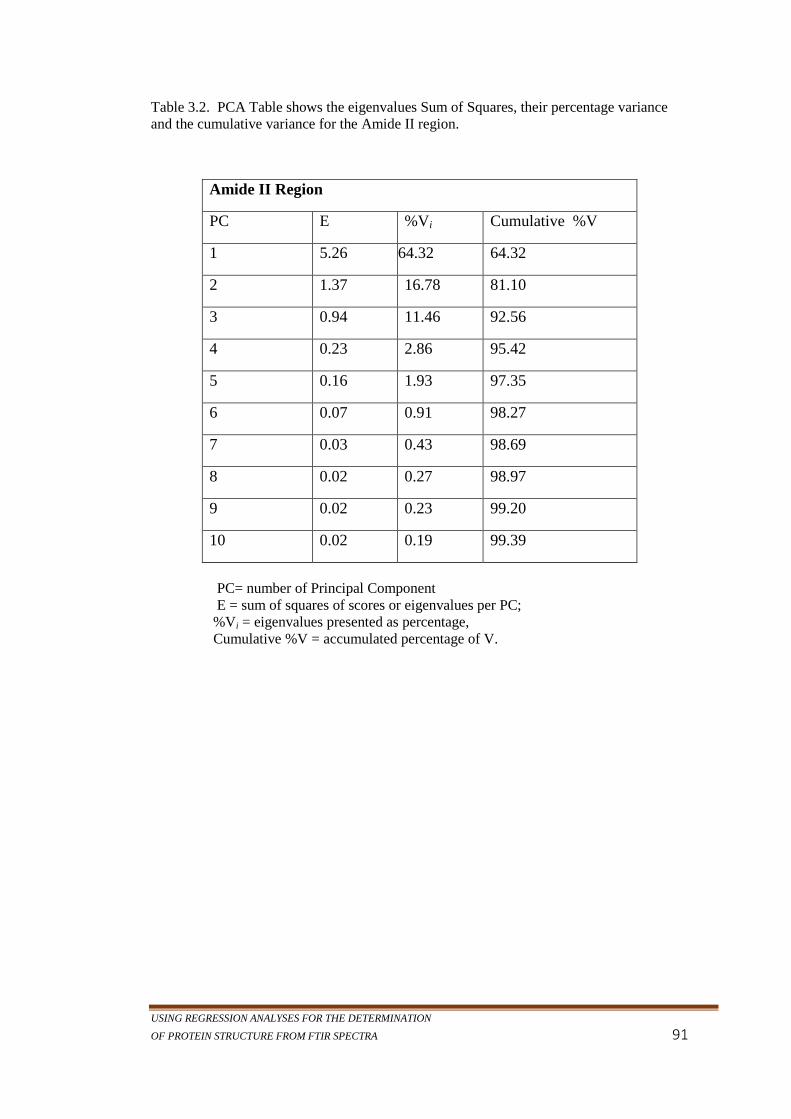
USING REGRESSION ANALYSES FOR THE DETERMINATION
OF PROTEIN STRUCTURE FROM FTIR SPECTRA 91
Table 3.2. PCA Table shows the eigenvalues Sum of Squares, their percentage variance
and the cumulative variance for the Amide II region.
Amide II Region
PC E %Vi Cumulative %V
1 5.26 64.32 64.32
2 1.37 16.78 81.10
3 0.94 11.46 92.56
4 0.23 2.86 95.42
5 0.16 1.93 97.35
6 0.07 0.91 98.27
7 0.03 0.43 98.69
8 0.02 0.27 98.97
9 0.02 0.23 99.20
10 0.02 0.19 99.39
PC= number of Principal Component
E = sum of squares of scores or eigenvalues per PC;
%Vi = eigenvalues presented as percentage,
Cumulative %V = accumulated percentage of V.

PROTEIN STRUCTURE CLASSIFICATION
92
-10
-8-6
-4-2
02
46
810
-4 -3 -2 -1 0 1 2 3 4
First
Princip
al C
om
ponent
Second Principal Component
annexi
nV
calm
odulin m
elit
tin
ferr
itin
rhodopsin
unble
ached
lysozym
em
yoglo
bin
hexa
kin
ase
porin phosvitin
nt-
anti-c
hym
otr
yp
pig
citra
te s
ynth
ase
alc
h-d
ehydro
g
alb
um
in (
sheep)
pero
xidase
phto
syste
m I
I ela
stin
lglu
tath
ion
concanavalin
avid
inapha-c
rysta
llin
chym
otr
ypsin
lactic d
ehydro
genase
pro
tein
ase
carb
onic
anhydra
se
trypsin
(hog)
trypsin
ogen
pepsin
ubiq
uitin
glu
cose o
xidase
split
- c1 inhib
itor
este
rase(b
.substilis
)
trypsin
transketa
lose
reaction c
ente
re R
. S
phae.
alp
ha c
asein
lipase w
heat
oth
er
Fig
ure
3.1
0. S
core
s plo
t fo
r A
mid
e II
reg
ion (
1480 c
m-1
– 1
600cm
-1)
of
spec
tra
of
pro
tein
s in
H2O
(P
C1
xP
C2
).
Plo
t sh
ow
s th
e cl
ust
erin
g o
f
score
s. B
lue
dots
are
pri
mar
ily α
-hel
ix r
ich
pro
tein
s, r
ed d
ots
are
pri
mar
ily β
-shee
t ri
ch pro
tein
s, a
nd
gre
en d
ots
in
dic
ate
pro
tein
s of
oth
er
stru
ctura
l ty
pes
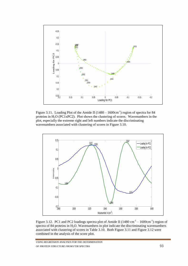
USING REGRESSION ANALYSES FOR THE DETERMINATION
OF PROTEIN STRUCTURE FROM FTIR SPECTRA 93
Figure 3.11. Loading Plot of the Amide II (1480 – 1600cm-1
) region of spectra for 84
proteins in H2O (PC1xPC2). Plot shows the clustering of scores. Wavenumbers in the
plot, especially the extreme right and left numbers indicate the discriminating
wavenumbers associated with clustering of scores in Figure 3.10.
Figure 3.12. PC1 and PC2 loadings spectra plot of Amide II (1480 cm-1
– 1600cm-1
) region of
spectra of 84 proteins in H2O. Wavenumbers in plot indicate the discriminating wavenumbers
associated with clustering of scores in Table 3.10. Both Figure 3.11 and Figure 3.12 were
combined in the analysis of the score plot.
-0.2-0.15-0.1-0.0500.050.10.150.2
-0.25
-0.2
-0.15
-0.1
-0.05
0
0.05
0.1
0.15
0.2
0.25
Loading for PC1
Loadin
g f
or P
C2
1553
1547
1523157215691567
1486
15501551
1555
15061583
1541
1480 1500 1520 1540 1560 1580 1600-0.2
-0.15
-0.1
-0.05
0
0.05
0.1
0.15
Wavenumber in (cm-1
)
Intensity
1522
1546
15671526
1571
1488
Loading for PC1
Loading for PC2

PROTEIN STRUCTURE CLASSIFICATION
94
3.6 Conclusion
ATR-FTIR spectroscopy is a useful tool for the analysis of proteins structure. Protein
amide vibrations are intrinsic to the backbone of the protein’s secondary structure. The
exact band position of the FTIR spectra is determined by the backbone conformation
and the hydrogen bonding pattern involved.(139) Another major contributing factor for
the amide vibration sensitivity to secondary structure is the transition dipole coupling of
the amide groups(the N-H bond) and their relative orientation and distance from one
another; this causes each secondary structure to absorb predominantly in a specific
spectral region helping to distinguish α-helix from β-sheet, etc.(140) The α-helix in the
Amide I absorption band is known to show up between 1655-1648 cm-1
while β-sheet
shows a strong band between 1648-1620 cm-1
.(50) However, the assignment of a band
to a secondary structure type is not straightforward because the bands largely overlap
and a broad band is observed as always seen in the amide I region; these bands can be
determined computationally by methods like curve fitting and multivariate analysis.
The analysis of the distribution of spectral signatures requires complex multivariate tool
like Principal Component Analysis (PCA).(119) Although protein spectra often look
similar, PCA clearly discriminates even structurally similar samples from each other as
was shown in the score plots. In our analysis we have investigated α+β and α/β SCOP
classes usually not considered for protein classification, and the results obtained were
significant.
PCA, an unsupervised pattern recognition technique, is a well-known method of
dimension reduction and data exploration. The basic principle of PCA is to reduce the
dimensionality of a data set, while retaining the variations present in the original
predictor variables (141). Due to the reduction in data, it is possible to graphically

USING REGRESSION ANALYSES FOR THE DETERMINATION
OF PROTEIN STRUCTURE FROM FTIR SPECTRA 95
explore the data correlation and understand the biological differences between protein
samples. Understanding these structural differences in proteins is important for the
proper classification of their biological differences.(142-144) With the help of methods
like PCA, analyses and visualization of the distribution of domains in a three
dimensional structure can be performed, so as to retrieve the important factors related to
protein function.(19, 143, 145)
The structural information in the protein spectra was retrieved primarily from the Amide
I bands, which arises chiefly from the C=O stretching vibrations between 1600 cm-1
and 1700 cm-1
, This region is used by spectroscopists for the study of proteins because
it contains a strong band frequency that is correlated to the secondary structure of
proteins.(134) The Amide I region has been used extensively for the study of protein
secondary structure because it presents the vibrational modes of different secondary
structures (α-helix, β-sheets, β-turns, coils etc.).(127) We have shown that ATR-FTIR
spectroscopy and PCA analysis can be combined successfully in the classification of
protein structure. In order to determine the identity of proteins, the score and the
loading plots of PCA analysis were employed as shown in Figure 3.2. The plot of PC1
versus PC2 plot revealed clusters of α-helix, β-sheets, α/β proteins, and α+β protein.
The loadings plot and loading spectra plots indicate that the most useful peaks in
distinguishing these structural regions, that is, the wavenumbers influence on each
spectrum makes it possible to identify the different classes and patterns of secondary
structures in the protein samples.
It can be shown that PCA loadings of ATR-FTIR spectra provide a basis for the
underlying differences between the identified protein structures (119, 146, 147), making

PROTEIN STRUCTURE CLASSIFICATION
96
it possible to disclose areas of the FTIR spectra that contribute the most to the variance
of the data in the Amide I and Amide II regions. The score plots provided by this PCA
analysis can be used as input to other classification methods; it can also be used to
check the structural grouping of unknown proteins before applying an appropriate
model to quantitatively determine their secondary structure compositions(127, 147-
149). Although PCA explores the structural relationships between data, it cannot be
used for the quantitative analysis of data, for this a different method called Partial Least
Squares is introduced in Chapter 4.
Table 3.3 summarizes the α-helix and β-sheet bands reported by other literature and
how the results from this analysis compare. Except for α/β, the other structure types are
well within the wavenumber ranges reported by the literature.
Table 3.3. FTIR marker bands of protein classes in the Amide I region.
Arrondo, Goni(50) Pelton, Mclean(137) This Work
Sec. Struct. Assign Infrared frequencies in cm -1
α-helix 1655-1648 1655-1650 1657
β-sheet 1648-1620
1693 (weak)
1640-1612 1685(weak) 1630
α+β 1690; 1630 1640-1612
1690-1670
1635
1674
α/β 1648; 1630 1640-1626 1653

USING REGRESSION ANALYSES FOR THE DETERMINATION
OF PROTEIN STRUCTURE FROM FTIR SPECTRA 97
4 PLS Regression for Protein Secondary Structure Determination
4.1 Introduction
The high quality of Fourier-Transform Infrared (FTIR) spectra has been used by many
spectroscopists for the analysis of protein secondary structure.(42, 150-154) It has
become a powerful tool in examining the conformation of proteins in H2O as well as in
D2O.(38) FTIR can rapidly obtain the biochemical fingerprint of samples under study
and give significant information on their biomolecule contents.(42, 155) Section 1.2
explained the importance of FTIR spectroscopy in more detail. This section will address
the quantitative determination of the secondary structural information present in the
infrared spectra of proteins. To determine the protein secondary structures from their
spectra, multivariate regression analysis methods such as Partial Least Squares (PLS)
and Principal Component Regression (PCR) were applied to the dataset of 84 FTIR
protein multivariate spectra with 16 proteins also measured in D2O, with the spectra
being collected and pre-processed as described in the ‘Pre-processing Method’ in
Chapter 2.
The Amide I region of the FTIR spectra is normally used in the analysis protein
secondary structure because the frequencies of the Amide I modes, which are due to
C=O stretching vibration, are known to correlate closely to a protein’s secondary
structure elements;(13, 156) however, the Amide I bands of proteins display extensive
overlaps of the underlying component bands of α-helix, β-sheet, β-turns and coils,
which are not instrumentally resolvable because they lie in too close proximity to each
other.(36) Therefore, mathematical methods, such as second derivatives, are often used
MULTIVARIATE ANALYSIS OF pH EFFECT 0N α-LACTALBUMIN
98
to enhance and resolve the individual band components corresponding to specific
secondary structures.(13) The application of 2nd
derivatives and pre-processing of the
proteins was described in Chapter 2.
The Amide I band components can be assigned by studying their frequency behaviour
in which the protein secondary structure is known by other techniques such as X-ray
crystallography.(157) A calibration model is determined from a set of samples, and the
X-ray known protein content and the resulting model is used to predict the content of
new, unknown samples from their spectra. In this chapter, PLS/PCR multivariate
calibration (using many variables simultaneously) was used to quantify new variables
‘y’ from the matrix of the FTIR measured protein spectra X, via a mathematical
function of some kind.(89) PLS and PCR solve the near multi-collinearity often found
in spectral measurements. This phenomenon has been explained in Chapter 1, it means
when two or more independent (predictor) variables are correlated and so provide
redundant information from the model. FTIR spectra are multivariate and collinear in
nature, therefore, the need for dimension reduction which is achieved by PLS
regression. The Capital letters ‘X’ is used to represent the entire matrix of protein
spectra while capital ‘Y’ represents a matrix of the dependent set, that is, the entire
secondary structure motif from X-ray crystallography. Small letters ‘x’ and ‘y’ are used
to represent a single vector from these matrices.
The PCR method is based on the basic concept of principal component analysis (PCA).
PCR performs data decomposition into loading and score variables used in building a
model. For PCR, the estimated scores matrix consists of the most dominating principal
components of X. These components are linear combinations of X measurements

USING REGRESSION ANALYSES FOR THE DETERMINATION
OF PROTEIN STRUCTURE FROM FTIR SPECTRA 99
determined by their ability to account for the variability in X.(158) The first principal
component is computed as the linear combination of the original X-variables with the
highest possible variance; PCR uses only the X variables for the analysis without
employing the y variable. On the other hand, PLS regression, which is similar to PCR,
can give good prediction results with fewer components than PCR because the response
variable is employed in the regression as well.(159) For detailed information on PLS
methodology, see Chapter 1, Multivariate Regression section. A consequence of this is
that the number of components needed for interpreting the information in X (measured
spectra) which is related to ‘y’ (reference secondary structure) is smaller for PLS than
for PCR. This may, in some cases, lead to simpler interpretation. Using the optimal
number of components in each case, however, the two methods often give comparable
prediction results.(13)
D2O has lower absorption around 1643-1650 cm-1
in the Amide I region which is where
proteins in H2O absorb water vapour;(117) however, H2O is preferred as a solvent for
the study of proteins because unlike D2O it does not modify the structure of
proteins.(53) Cell fluid is made up of high water content and water is less expensive to
work with. The proteins in D2O were analysed for their secondary content to compare
and evaluate the results produced from the regression method employed.
4.2 Protein dataset used for this method
The dataset of proteins used for this study has been described in the Chapter 3 which
covered PCA; this was also covered in Chapter 2 which explained the pre-processing
done for this project.. The dataset represents a wide range of helix and sheet fractional
content values and other structural contents such as 310-helix, turns and unordered

MULTIVARIATE ANALYSIS OF pH EFFECT 0N α-LACTALBUMIN
100
structure as described and determined by the Dictionary of Protein Secondary Structure
(DSSP) (109). The selection of these protein samples was based on criteria such as
crystal structure quality and the distribution of their secondary structures,
conformational classes as described by the Structural Classification of Protein (SCOP)
system,(18) and protein solubility and stability. These 84 proteins measured in H2O and
16 selected proteins measured in D2O are listed in Tables 1a-f and 2a-c in Appendix-B.
All spectra were pre-treated by means of intensity normalization and SNV (Standard
Normal Variate) as described in Chapter 1, section 1.3.
Data Selection Scheme 4.2.1
Models generated from the PLS/PCR methods were used for the prediction of the
structural compositions of new samples; therefore, as many possible biochemical
compositions of protein samples and types of protein structure that could be
encountered later should be represented in the calibration set.(160) From the ‘X’ and
‘y’ matrices of the calibration set of proteins in H2O, 60 spectra were used to develop
the partial least squares regression model. The remaining 24 were used as the
independent test set, set aside for predictive accuracy. Of the training set, 20 were
included in the test set for validation accuracy, totalling 44 samples in the test set. This
selection was done by an algorithm called Kennard Stone (KS).(161) KS is a well-
known method for the selection of a sample subset for calibration. It chooses objects
that are uniformly distributed in the X-matrix (the measured spectra) by assigning a
sample to the calibration set, closest to the mean of the entire sample; the next sample is
then chosen based on the square distance to the sample already assigned.(162) The
sample furthest from the already selected sample is added to the calibration set, etc. In
this way, variations of the dataset are chosen up front. The algorithm was set to select

USING REGRESSION ANALYSES FOR THE DETERMINATION
OF PROTEIN STRUCTURE FROM FTIR SPECTRA 101
the first 60 samples representing the dataset, with the rest left for validation. The
calibration model was constructed and subsequently validated. Figure 4.1 represents
the KS selections split into calibration set and test set.
Figure 4.1. Schematic representation of samples used in the training set and the test set
after application of the Kennard Stone selection algorithm. Matrix X represents the FTIR
spectra while vector ‘y’ represents the percentage fraction of structure determined by DSSP
analysis from X-ray crystallographic data. This figure represents the strategy for the 84
protein samples measured in H2O.
4.3 PLS Modelling
The PLS model is a mathematical representation of a complicated system that holds
within it the information of the contents of that system,(89, 155, 163, 164) in this case,
protein secondary structure. Sample preparation and ATR-FTIR spectral collection for
this experiment are described in sections 2.2 and 2.3. Data points in the ATR-FTIR
40 proteins for calibration set
24 proteins to test set
1
2
.
.
.
.
.
.
.
.
.
.
.
.
.
.
. 84
20 used in both
60 proteins
44 proteins
40
24
20
Matrix X Vector y

MULTIVARIATE ANALYSIS OF pH EFFECT 0N α-LACTALBUMIN
102
spectra, as described in section 3.2, were first normalized before calculating the second
derivative which is done in order to enhance the separation of the underlying bands.
As in the PCA section, the Amide I region, whose bands mostly originates from C=O
stretching vibrations, and Amide II region, mostly arising from NH bending vibrations,
were used for this analysis. The Amide III region was not recorded in many of the
protein spectra used for this study; therefore this region was not analysed here.
The FTIR spectra were put into a matrix form containing 84 rows made of the measured
protein spectral intensities and 101 columns made up of the spectral wavenumbers in
the Amide I region and a separate matrix form of 124 columns for the Amide II region
of the spectra for Amide II analysis. The algorithm for PLS was written using Matlab
R2010 and Matlab’s PLSregression. PLS requires a priori knowledge about the protein
structural groups; fractions of the proteins secondary structure (SS) motifs have been
determined by X-ray crystallography and files of their atomic features obtained from the
Protein Data Bank (PDB)(137, 157, 165) were fed into a DSSP script, output from
DSSP contains the proteins’ secondary structure information which was put into a
matrix form labelled as ‘y’ These SS fractions are listed in Table A2, Appendix A.
PLS regression was applied to determine secondary structure contents using the Amide I
regions (1700-1600 cm-1
region) and Amide II bands (1600–1480 cm 1) of the spectra
separately and to the Amide I & II regions together to determine and compare their
secondary structural compositions to that determined by X-ray crystallography. PLS
finds the optimal linear combination of the variables in the obtained FTIR spectra of
protein samples (X variables) and these linear combination variables, called components

USING REGRESSION ANALYSES FOR THE DETERMINATION
OF PROTEIN STRUCTURE FROM FTIR SPECTRA 103
but also known as latent variables (LV)(105), were used to determine the regression
equation (2.2). The general equation notation is:
Y = Xb + ε, where eq. (4.1)
Y is the matrix of the predicted latent variables, X is the predictor latent variable,
b is the determined coefficients during calibration, and ε is the residual error (the
difference between the observed and predicted dependent variables).
4.4 Results and Discussions
A plot of the ‘percentage of y explained variance’ based on chosen components, as seen
in Figure 4.2, was obtained. The diagnostics from this plot were used to choose a
different model; that is, based on the plotted percentage y explained variance, a
minimum number of components that gave rise to the maximum explained variance was
chosen for each analysed region of the spectra. PLS extracts components in order of
their relevance to the structure type in question.(127, 152) From Figure 4.2 and Figure
4.3 for α-helix, we see that after 10 components the gap between points got smaller and
the line curvature begins to flatten. Any value between 6 and 10 could have been
chosen for the model, validation of this model was done later to eliminate overfitting
issues. 10 components for the analysis α-helix from the Amide I region was selected as
the maximum explanation of variance and a low Root Mean Square Error for
Calibration (RMSEC).

MULTIVARIATE ANALYSIS OF pH EFFECT 0N α-LACTALBUMIN
104
Figure 4.2. Explained Y variance of α-helix for Amide I region; explained variance is
about 96% for 10 components.
Figure 4.3. Plot shows Root Mean Square Error (RMSE) vs. number of components for α-
helix of the Amide I region. 10 components gave low root mean square error and was
chosen to fit the data.
0 5 10 150
20
40
60
80
100
Number of PLS components
% V
aria
nce E
xpla
ined in
y
0 5 10 150
0.01
0.02
0.03
0.04
0.05
Number of PLS components
Root M
ean S
quare E
rror

USING REGRESSION ANALYSES FOR THE DETERMINATION
OF PROTEIN STRUCTURE FROM FTIR SPECTRA 105
Figure 4.4 and Figure 4.5 also show that 10 components for analysis of β-sheet content
from the Amide I gave the maximum explanation of variance at a low Root Mean
Square Error for Calibration (RMSEC) of 0.020. This is the maximum number of
components before the decrease in the RMSEC is negligible. It is assumed that this
number will fit new samples, however, a cross-validation was later performed to
eliminate the need to keep adding unnecessary PLS components to the model. Looking
at the RMSEC plot, anywhere between 7-10 components would be suitable for
providing a good estimate.
Figure 4.4. Explained Y variance of β-sheet for the Amide I region is about 95 % for 10
components.
0 5 10 1540
50
60
70
80
90
100
Number of PLS components
% V
aria
nce E
xpla
ined in y

MULTIVARIATE ANALYSIS OF pH EFFECT 0N α-LACTALBUMIN
106
Figure 4.5. Root Mean Square Error for β-sheet analysis for the Amide I region.
Model Validation 4.4.1
PLS is sensitive to overfitting, that is, the RMSEC will continue to decrease for
additional PLS factors (components) chosen for the model; however, the Root Mean
Square Error for Prediction (RMSEP) will continue to increase due to overfitting.(99)
For this reason cross-validation of the model is carried out to ensure that obtained
results are not from random noise. The test samples left out of the calibration set were
used as the validation set. The predicted ‘y’ values of these new samples are compared
to that of the true ‘y’ values and the predictive ability of the model was then calculated.
Cross-Validation 4.4.2
Models were cross-validated and an optimal number of latent variables, indicated by a
minimum root mean square error of cross-validation (RMSECV),was selected to avoid
overfitting.(100-102) For PLS, this error measurement, which is the standard deviation
0 5 10 150
0.005
0.01
0.015
0.02
0.025
Number of PLS components
Ro
ot
Me
an
Sq
uare
Erro
r

USING REGRESSION ANALYSES FOR THE DETERMINATION
OF PROTEIN STRUCTURE FROM FTIR SPECTRA 107
of the unexplained variance of the cross-validation, is a much better fit than RMSEC
because RMSEC does not indicate when the model is overfitted.
Overfitting occurs when too many components are selected to fit the model as this can
lead to much redundancy in the ‘x’ variables resulting in a higher estimation error due
to data dependency. Cross-validation (CV) is used to choose the optimal number of
components to use for the model and to check on overfitting by not reusing the same
data for calibration and prediction error.(166) With a “Leave One Out” cross-
validation, one data item at a time from the n samples is left out of fitting (n-1), and
error estimation and calibration is performed on the rest of the data. The deleted data
are put back for calibration and another sample is taken out.(100) These samples left
out are used as test samples. In this method a “CV” option was given to the MATLAB
PLS function with 10-fold (segments) specified. "CV" divides the randomly selected
data into 10 segments and each segment was left out one at a time. Plots of the
validation results are used to visualize the number of components that give the lowest
Root Mean Square Error for Cross Validation (RMSECV). Figure 4.6 shows that the
optimum number of components, 4, was enough to fit the spectra of new samples.
The RMSECV (see eq. 4.2) must be interpreted in a slightly different way to Root Mean
Square Error of the Prediction (RMSEP). Note, in particular, that it is not an error
estimate of an actual predictor with already computed regression coefficients. Cross-
validation provides, instead, an estimate of the average prediction error of calibration
equations based on N-1 samples drawn from the actual population of samples.
Eq. (4.2)

MULTIVARIATE ANALYSIS OF pH EFFECT 0N α-LACTALBUMIN
108
RMSECV = √∑(𝑦𝑝𝑟𝑒𝑑
𝑐𝑣,𝑖 −𝑦𝑜𝑏𝑠𝑖 )
2
𝑛−1
𝑛𝑖=1 eq. (4.2)
where n is the number of proteins in the dataset, ypred is the predicted Figure and yobs is
the observed value from X-ray crystallography.
Figure 4.6. CV cross-validation: 4 PLS components only are required to fit the α-helix
model for proteins in H2O for the Amide I region.
Independent Test Set 4.4.3
Cross-validation does an internal test with the calibration model; therefore, it is always
useful to test out a model against an independent test set. For the model that has already
been established, the prediction ability, and not the fitting ability, indicates how well the
model can predict new samples that have not been seen by the model.(167, 168) The
best way to perform this validation is by using the 44 samples in the test set not
previously used. By predicting the ‘y’ values of the samples in the test set and then
comparing the results with the true values, an estimate of the predictive ability of the
0 5 10 15 200.02
0.04
0.06
0.08
0.1
0.12
0.14
0.16
Number of PLS components
RM
SE
CV
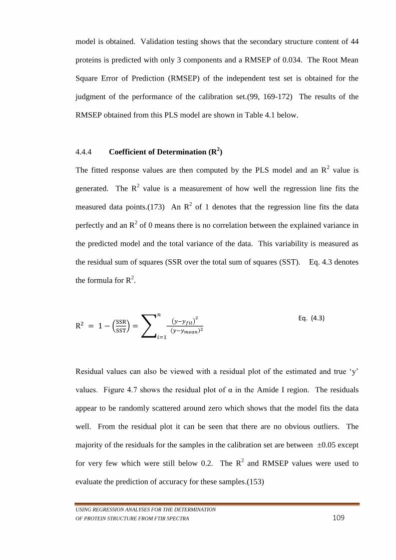
USING REGRESSION ANALYSES FOR THE DETERMINATION
OF PROTEIN STRUCTURE FROM FTIR SPECTRA 109
model is obtained. Validation testing shows that the secondary structure content of 44
proteins is predicted with only 3 components and a RMSEP of 0.034. The Root Mean
Square Error of Prediction (RMSEP) of the independent test set is obtained for the
judgment of the performance of the calibration set.(99, 169-172) The results of the
RMSEP obtained from this PLS model are shown in Table 4.1 below.
Coefficient of Determination (R2) 4.4.4
The fitted response values are then computed by the PLS model and an R2 value is
generated. The R2 value is a measurement of how well the regression line fits the
measured data points.(173) An R2 of 1 denotes that the regression line fits the data
perfectly and an R2 of 0 means there is no correlation between the explained variance in
the predicted model and the total variance of the data. This variability is measured as
the residual sum of squares (SSR over the total sum of squares (SST). Eq. 4.3 denotes
the formula for R2.
R2 = 1 − (SSR
SST) = ∑
(𝑦−𝑦𝑓𝑖𝑡)2
(𝑦−𝑦𝑚𝑒𝑎𝑛)2
𝑛
𝑖=1
Residual values can also be viewed with a residual plot of the estimated and true ‘y’
values. Figure 4.7 shows the residual plot of α in the Amide I region. The residuals
appear to be randomly scattered around zero which shows that the model fits the data
well. From the residual plot it can be seen that there are no obvious outliers. The
majority of the residuals for the samples in the calibration set are between ±0.05 except
for very few which were still below 0.2. The R2 and RMSEP values were used to
evaluate the prediction of accuracy for these samples.(153)
Eq. (4.3)

MULTIVARIATE ANALYSIS OF pH EFFECT 0N α-LACTALBUMIN
110
Figure 4.7. Residual plot of the 60 samples in the Amide I region. Error levels between
the fit and the individual data are shown for each sample. Note: The residuals are not
sorted by protein but by the order in which they were analysed.
PCR 4.4.5
The major difference between PLS and PCR is that PCR uses only the X variables for
the analysis without employing the y variable, although the y response variable is
needed for the calculation of the residual. A comparison of PLS and PCR was made to
see which method works best for the analysis of protein secondary structure.
For our data calibration, PLS and PCR cross-validation were plotted for comparison.
This plot is shown in Figure 4.8. The plot suggests that as few as 3 PLS components
may be adequate to interpret the information in the predictor (X) which is related to the
response (y), but 5 PCR components were required. PCR constructs components to
0 10 20 30 40 50 60-0.15
-0.1
-0.05
0
0.05
0.1
0.15
0.2
Observation
Resid
ual
albumin (sheep)
glucose oxidase (aspegillus niger)Aprotinin (bovine lung)
thaumactin (t.danielli)

USING REGRESSION ANALYSES FOR THE DETERMINATION
OF PROTEIN STRUCTURE FROM FTIR SPECTRA 111
explain the data in the calibration set without much regard to the reference set values
(y), while PLS puts the reference set values into consideration while fitting, and, as a
result, PCR requires more components to fit the data. As the number of components
increases, the two methods often give similar prediction results or PCR may do better.
As seen in Figure 4.8, it appears that the PLS cross-validation (PLS-CV) technique is
more realistic to test the predictive ability. This is not always the case for all secondary
structure results in this analysis. See Section 4.4.8 and Tables 4.1a/b.
Figure 4.8. Performance of CV cross-validation: 4 PLS components is optimal for PLS-
CV while 5 components is optimal for PCR-CV (Amide I region of FTIR spectra).
PLS with 2nd
Derivative 4.4.6
Second derivative spectra did better with fewer components in the calibration of the
entire spectra (combined Amide I and II regions). The plotted observed vs. fitted
response in Figure 4.9 for proteins in H2O solution shows that the regression line fits the
data very well for α-helix and β-sheet from bands in the Amide I region. Datasets
1 2 3 4 5 6 7 8 9 10 110.01
0.02
0.03
0.04
0.05
0.06
Number of CV components
RM
SE
CV
PLS-crossvalidation
PCR-crossvalidation

MULTIVARIATE ANALYSIS OF pH EFFECT 0N α-LACTALBUMIN
112
computed from the second derivatives of the FTIR spectra were used for secondary
structure analysis with a PLS calibration. The R2 and RMSECV values for each
calibration were used in choosing the best fit model in the spectral range of α-helix, β-
sheet, parallel β-sheet, anti-parallel β-sheet, β-turns and “other”. These results can be
seen in the highlighted rows of Table 4.1.
The PLS analysis of the 2nd
derivative of Amide I data used 10 components for the
prediction of α-helix content, giving an R2 of 96% with a low RMSEC of 0.040 which,
after cross-validation, gave an RMSECV value of 0.185 with only 4 components. This
is an ideal number of PLS components for the final model because cross-validation
choses optimal components that ensure no overfitting of the model. This number of
components was found by the low values of the estimated RMSECV and was used to
predict α-helix in the test set, giving a RMSEP of 0.120 with an R2 of 71%. The fit of
the data in the test set for α-helix prediction from the Amide I region is plotted (see
Figure 4.10) and the predicted result of each individual sample can be seen in Tables
B1-B6 in Appendix B. Figures 4.11 and 4.12 show the fitted vs observed plots for the
β-sheet calibration and test sets of data from the Amide I region of the FTIR protein
spectra using the same method.

USING REGRESSION ANALYSES FOR THE DETERMINATION
OF PROTEIN STRUCTURE FROM FTIR SPECTRA 113
Figure 4.9. The plot of the calibration set for the analysis of α-helix content from Amide
I region : This plot shows PLS fitted vs response (X-ray crystallography values) using the
FTIR spectra of 60 proteins in H2O for calibration. The red line of fit going through the
origin emphasises the positive correlation in the data.
Figure 4.10. Test set plot for analysis of α-helix from the Amide I data: PLS fitted vs
response on 44 proteins in H2O used for testing the model. The model shows the
relationship between the crystal structure values and the calculated values of α-helix from
FTIR spectra for these proteins.
0 0.1 0.2 0.3 0.4 0.5 0.6 0.7 0.8 0.9 1-0.2
0
0.2
0.4
0.6
0.8
1
1.2
-helix train set values
predic
ted valu
es
0 0.1 0.2 0.3 0.4 0.5 0.6 0.7 0.8 0.9 1-0.2
0
0.2
0.4
0.6
0.8
1
1.2
-helix test set values
predic
ted valu
es

MULTIVARIATE ANALYSIS OF pH EFFECT 0N α-LACTALBUMIN
114
Figure 4.11. Plot shows PLS prediction for β-sheet vs. X-ray crystallography vales used in
the training of the Amide I region. The training set had FTIR spectra of 60 proteins in
H2O. The red line of fit going through the origin emphasises the positive correlation in the
data.
Figure 4.12. Test set plot of Amide I β-sheet: PLS fitted vs response on 44 proteins in
H2O used for testing the model.
0 0.1 0.2 0.3 0.4 0.5 0.6 0.7 0.8 0.9 1-0.2
0
0.2
0.4
0.6
0.8
1
1.2
-sheet train set values
predic
ted valu
es
0 0.1 0.2 0.3 0.4 0.5 0.6 0.7 0.8 0.9 10
0.2
0.4
0.6
0.8
1
-sheet test set values
predic
ted valu
es
USING REGRESSION ANALYSES FOR THE DETERMINATION
OF PROTEIN STRUCTURE FROM FTIR SPECTRA 115
Eq. (4.4)
Calibration of each of these secondary structural contents was done for both the entire
Amide I and Amide II regions separately and for the combined Amide I and II regions
together, as is shown in Table 4.1. Cross-validation R2 results of 0.88 (α-helix), 0.94
(β-sheet), 0.44 (parallel β-sheet), 0.93 (antiparallel β-sheet), 0.44 (mixed β-sheet), 0.53
(310-helix), 0.60 (turns), and 0.62 (other) for the Amide I region indicates the percentage
explained variance of each predicted structure. The RMSECV must be interpreted
differently, as it is an estimate of the average internal prediction error whereas RMSEC
is an error estimate of the calibration. Note that the RMSECV values for α-helix
(0.185) and β-sheet (0.111) are higher than the ones for parallel β-sheet (0.052), 310-
helix (0.037), and turns (0.051). This is not because the predictive values of the later
are better, but rather that, in our samples, the variations of parallel β sheet, 310-helix and
turns are small with an average of 10% 310-helix content and 3% parallel β- sheet for the
measured proteins. To assess the predictive accuracy of this statistical analysis, a
determinant ‘ζ’ has been calculated and presented alongside with the RMSECV.
Zeta scores ζ 4.4.7
The RMSE of cross-validation and how it relates to the standard deviation of the
reference (crystal) structure(s) is calculated as the ratio of RMSECV (δ) of the FTIR
structure divided by the standard deviation (σ) of the crystal structure.(174) that is, the
standard deviation of the protein secondary structure motif in the reference set;
therefore,
ζ = (δFTIR/ σy) eq. (4.4)
MULTIVARIATE ANALYSIS OF pH EFFECT 0N α-LACTALBUMIN
116
This score compares the distributed width of the reference structure to that of the
RMSECV and is used to compare the prediction accuracy as it accounts for the natural
variation of the crystal structure data to that of the calculated structure obtained from the
FTIR/PLS model. (175, 176) A ζ value of one indicates that the secondary structure
prediction is as accurate as what would be found from any random guess for the average
value.(174, 175) A value less than one indicates that the FTIR prediction values of that
structure are better than the value from X-ray crystallography for that structure and a
value around one means both methods give answers that are comparable. A value much
higher than one indicates that the performance of the crystal structure data is
better.(175, 177) Sometimes the formula above (in eq. 4.4.) is inverted so that the
standard deviation of the crystal structure is divided by the calculated RMSE of the
FTIR structure. In either case, if the calculated value is less than 1 the numerator is the
better predictor but if the value is greater than 1, the denominator is assigned as the
better predictor. Using equation 4.4 the ζ scores for α-helix, β-sheet, and parallel β-
sheet from the Amide I data are comparable to that from their crystal structures. The ζ
values for data in the Amide I & II regions together also gave good predictions for the
same secondary structures. The two scores, RMSECV and ζ, should both be considered
because a secondary structure with few samples in the data space could give a low
RMSE and ζ would indicate this case.
PCR/PLS comparison 4.4.8
In Figure 4.8, it was seen that it took 5 PCR components to give a low RMSECV. As
the object of this comparison is to show the difference in fitting between PLS and PCR
with similar components, this was done using normalized SNV data alone.
Normalization of spectral intensity and use of Singular Value Decomposition (SNV)
have been introduced and explained in the Multivariate Analysis section of Chapter 1.

USING REGRESSION ANALYSES FOR THE DETERMINATION
OF PROTEIN STRUCTURE FROM FTIR SPECTRA 117
The use of ‘Normalized +SNV’ for this comparison also showcases the difference in
performance between this type of pre-processing and the ‘Normalized + 2nd
Derivative’
method (Table 4.1). PCR produced a lower RMSECV for cross-validation (0.104) and
a ζ score of 0.437 for α-helix compared to PLS (SNV) cross-validation values of 0.143
and a ζ score of 0.603; PLS with 2nd
derivative gave RMSECV of 0.181 and ζ score of
0.794 however the calibration and prediction with the independent testset gave better
values than PCR and PLS (SNV), see Table 4.1a for α-helix. The α-helix ζ score was
derived from dividing RMSECV by the standard deviation of the α-helix motif of the
crystal structure used in the reference set; this is done for all secondary structure. ζ is
explained in section 4.4.7.
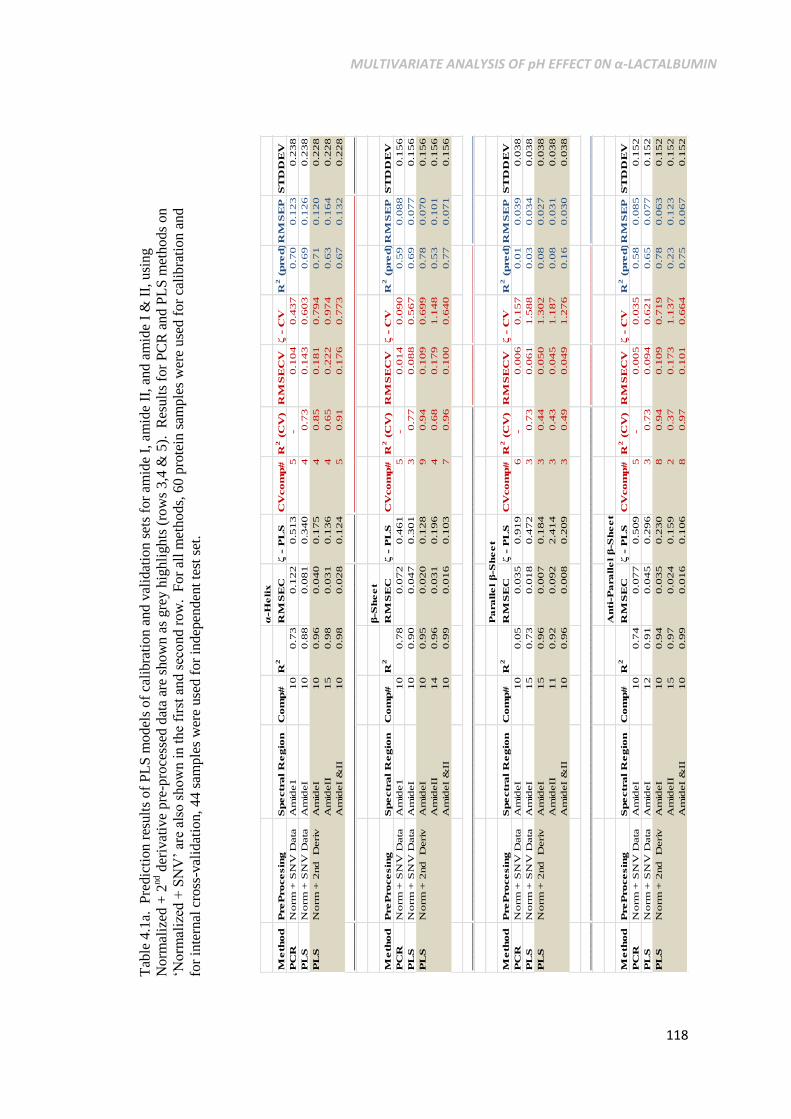
MULTIVARIATE ANALYSIS OF pH EFFECT 0N α-LACTALBUMIN
118
α-H
elix
Meth
od
PreP
ro
cesin
gS
pectr
al R
eg
ion
Co
mp#
R2
RM
SE
Cζ -
PL
SC
Vco
mp#
R2 (
CV
)R
MS
EC
Vζ -
CV
R2 (
pred)R
MS
EP
ST
DD
EV
PC
RN
orm
+ S
NV
Data
Am
ide1
10
0.7
30.1
22
0.5
13
5-
0.1
04
0.4
37
0.7
00.1
23
0.2
38
PL
SN
orm
+ S
NV
Data
Am
ideI
10
0.8
80.0
81
0.3
40
40.7
30.1
43
0.6
03
0.6
90.1
26
0.2
38
PL
SN
orm
+ 2
nd
D
eriv
Am
ideI
10
0.9
60.0
40
0.1
75
40.8
50.1
81
0.7
94
0.7
10.1
20
0.2
28
Am
ideII
15
0.9
80.0
31
0.1
36
40.6
50.2
22
0.9
74
0.6
30.1
64
0.2
28
Am
ideI
&II
10
0.9
80.0
28
0.1
24
50.9
10.1
76
0.7
73
0.6
70.1
32
0.2
28
__________
_______________________________________________________________________________________________________________
________
_______________________________________________________________
_________
β-S
heet
Meth
od
PreP
ro
cesin
gS
pectr
al R
eg
ion
Co
mp#
R2
RM
SE
Cζ -
PL
SC
Vco
mp#
R2 (
CV
)R
MS
EC
Vζ -
CV
R2 (
pred)R
MS
EP
ST
DD
EV
PC
RN
orm
+ S
NV
Data
Am
ide1
10
0.7
80.0
72
0.4
61
5-
0.0
14
0.0
90
0.5
90.0
88
0.1
56
PL
SN
orm
+ S
NV
Data
Am
ideI
10
0.9
00.0
47
0.3
01
30.7
70.0
88
0.5
67
0.6
90.0
77
0.1
56
PL
SN
orm
+ 2
nd
D
eriv
Am
ideI
10
0.9
50.0
20
0.1
28
90.9
40.1
09
0.6
99
0.7
80.0
70
0.1
56
Am
ideII
14
0.9
60.0
31
0.1
96
40.6
80.1
79
1.1
48
0.5
30.1
01
0.1
56
Am
ideI
&II
10
0.9
90.0
16
0.1
03
70.9
60.1
00
0.6
40
0.7
70.0
71
0.1
56
__________
_______________________________________________________________________________________________
_____________________________________________
__________________
_________________
Pa
ra
llel β-S
heet
Meth
od
PreP
ro
cesin
gS
pectr
al R
eg
ion
Co
mp#
R2
RM
SE
Cζ -
PL
SC
Vco
mp#
R2 (
CV
)R
MS
EC
Vζ -
CV
R2 (
pred)R
MS
EP
ST
DD
EV
PC
RN
orm
+ S
NV
Data
Am
ideI
10
0.0
50.0
35
0.9
19
6-
0.0
06
0.1
57
0.0
10.0
39
0.0
38
PL
SN
orm
+ S
NV
Data
Am
ideI
15
0.7
30.0
18
0.4
72
30.7
30.0
61
1.5
88
0.0
30.0
34
0.0
38
PL
SN
orm
+ 2
nd
D
eriv
Am
ideI
15
0.9
60.0
07
0.1
84
30.4
40.0
50
1.3
02
0.0
80.0
27
0.0
38
Am
ideII
11
0.9
20.0
92
2.4
14
30.4
30.0
45
1.1
87
0.0
80.0
31
0.0
38
Am
ideI
&II
10
0.9
60.0
08
0.2
09
30.4
90.0
49
1.2
76
0.1
60.0
30
0.0
38
__________
_______________________________________________________________________________________________
_____________________________________________
__________________
_________________
Anti
-Pa
ra
llel β-S
heet
Meth
od
PreP
ro
cesin
gS
pectr
al R
eg
ion
Co
mp#
R2
RM
SE
Cζ -
PL
SC
Vco
mp#
R2 (
CV
)R
MS
EC
Vζ -
CV
R2 (
pred)R
MS
EP
ST
DD
EV
PC
RN
orm
+ S
NV
Data
Am
ideI
10
0.7
40.0
77
0.5
09
5-
0.0
05
0.0
35
0.5
80.0
85
0.1
52
PL
SN
orm
+ S
NV
Data
Am
ideI
12
0.9
10.0
45
0.2
96
30.7
30.0
94
0.6
21
0.6
50.0
77
0.1
52
PL
SN
orm
+ 2
nd
D
eriv
Am
ideI
10
0.9
40.0
35
0.2
30
80.9
40.1
09
0.7
19
0.7
80.0
63
0.1
52
Am
ideII
15
0.9
70.0
24
0.1
59
20.3
70.1
73
1.1
37
0.2
30.1
23
0.1
52
Am
ideI
&II
10
0.9
90.0
16
0.1
06
80.9
70.1
01
0.6
64
0.7
50.0
67
0.1
52
Tab
le 4
.1a.
P
redic
tion
res
ult
s o
f P
LS
model
s of
cali
bra
tion a
nd v
alid
atio
n s
ets
for
amid
e I,
am
ide
II,
and
am
ide
I &
II,
usi
ng
Norm
aliz
ed +
2nd d
eriv
ativ
e p
re-p
roce
ssed
dat
a ar
e sh
ow
n a
s gre
y h
ighli
ghts
(ro
ws
3,4
& 5
).
Res
ult
s fo
r P
CR
an
d P
LS
met
ho
ds
on
‘Norm
aliz
ed +
SN
V’
are
also
sh
ow
n i
n t
he
firs
t an
d s
eco
nd r
ow
. F
or
all
met
hods,
60 p
rote
in s
amp
les
wer
e u
sed
for
cali
bra
tio
n a
nd
for
inte
rnal
cro
ss-v
alid
atio
n, 4
4 s
ample
s w
ere
use
d f
or
indep
enden
t te
st s
et.
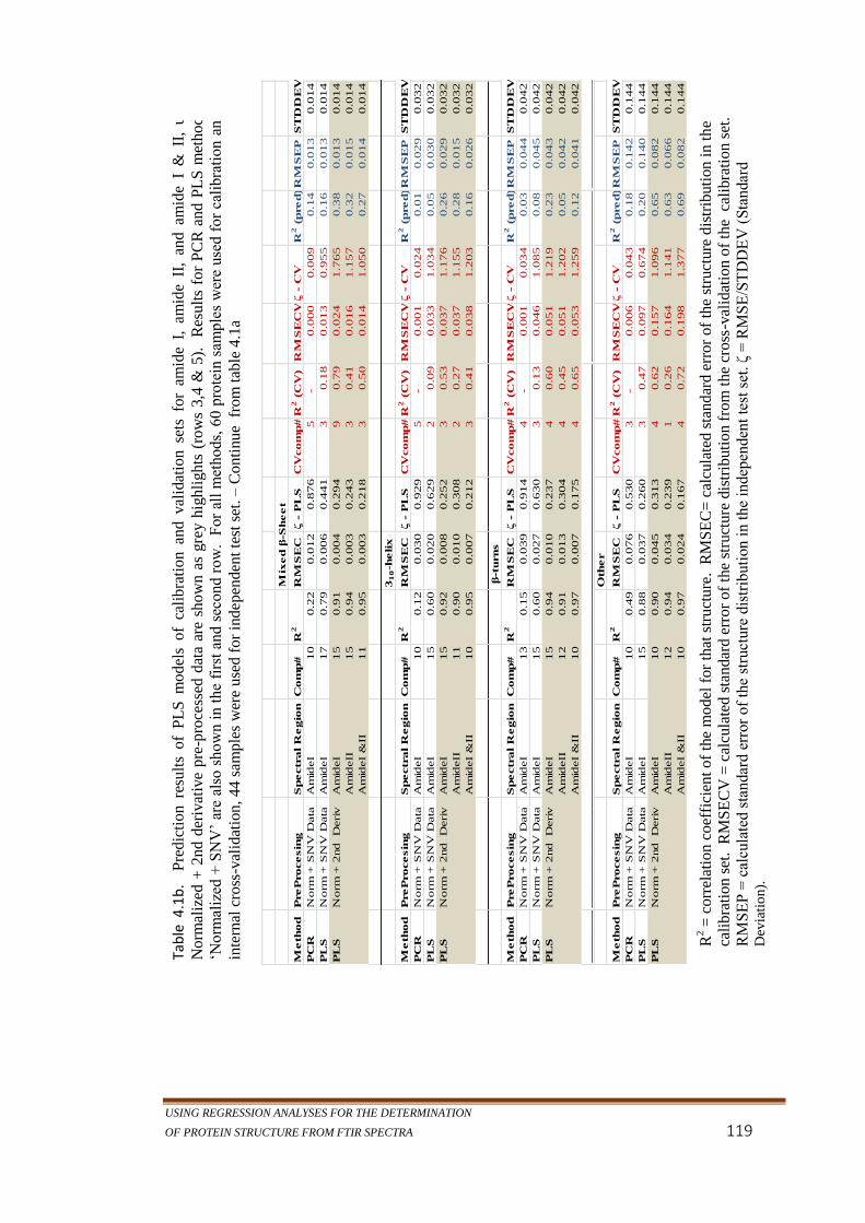
USING REGRESSION ANALYSES FOR THE DETERMINATION
OF PROTEIN STRUCTURE FROM FTIR SPECTRA 119
Mix
ed β
-Sheet
Meth
od
PreP
rocesin
gS
pectr
al R
egio
nC
om
p#
R2
RM
SE
Cζ -
PL
SC
Vcom
p#
R2 (
CV
)R
MS
EC
Vζ -
CV
R2 (
pred)R
MS
EP
ST
DD
EV
PC
RN
orm
+ S
NV
Data
Am
ideI
10
0.2
20.0
12
0.8
76
5-
0.0
00
0.0
09
0.1
40.0
13
0.0
14
PL
SN
orm
+ S
NV
Data
Am
ideI
17
0.7
90.0
06
0.4
41
30.1
80.0
13
0.9
55
0.1
60.0
13
0.0
14
PL
SN
orm
+ 2
nd D
eriv
Am
ideI
15
0.9
10.0
04
0.2
94
90.7
90.0
24
1.7
65
0.3
80.0
13
0.0
14
Am
ideII
15
0.9
40.0
03
0.2
43
30.4
10.0
16
1.1
57
0.3
20.0
15
0.0
14
Am
ideI
&II
11
0.9
50.0
03
0.2
18
30.5
00.0
14
1.0
50
0.2
70.0
14
0.0
14
31
0-h
elix
Meth
od
PreP
rocesin
gS
pectr
al R
egio
nC
om
p#
R2
RM
SE
Cζ -
PL
SC
Vcom
p#
R2 (
CV
)R
MS
EC
Vζ -
CV
R2 (
pred)R
MS
EP
ST
DD
EV
PC
RN
orm
+ S
NV
Data
Am
ideI
10
0.1
20.0
30
0.9
29
5-
0.0
01
0.0
24
0.0
10.0
29
0.0
32
PL
SN
orm
+ S
NV
Data
Am
ideI
15
0.6
00.0
20
0.6
29
20.0
90.0
33
1.0
34
0.0
50.0
30
0.0
32
PL
SN
orm
+ 2
nd D
eriv
Am
ideI
15
0.9
20.0
08
0.2
52
30.5
30.0
37
1.1
76
0.2
60.0
29
0.0
32
Am
ideII
11
0.9
00.0
10
0.3
08
20.2
70.0
37
1.1
55
0.2
80.0
15
0.0
32
Am
ideI
&II
10
0.9
50.0
07
0.2
12
30.4
10.0
38
1.2
03
0.1
60.0
26
0.0
32
β-t
urns
Meth
od
PreP
rocesin
gS
pectr
al R
egio
nC
om
p#
R2
RM
SE
Cζ -
PL
SC
Vcom
p#
R2 (
CV
)R
MS
EC
Vζ -
CV
R2 (
pred)R
MS
EP
ST
DD
EV
PC
RN
orm
+ S
NV
Data
Am
ideI
13
0.1
50.0
39
0.9
14
4-
0.0
01
0.0
34
0.0
30.0
44
0.0
42
PL
SN
orm
+ S
NV
Data
Am
ideI
15
0.6
00.0
27
0.6
30
30.1
30.0
46
1.0
85
0.0
80.0
45
0.0
42
PL
SN
orm
+ 2
nd D
eriv
Am
ideI
15
0.9
40.0
10
0.2
37
40.6
00.0
51
1.2
19
0.2
30.0
43
0.0
42
Am
ideII
12
0.9
10.0
13
0.3
04
40.4
50.0
51
1.2
02
0.0
50.0
42
0.0
42
Am
ideI
&II
10
0.9
70.0
07
0.1
75
40.6
50.0
53
1.2
59
0.1
20.0
41
0.0
42
__________
_______________________________________________________________________________________________
_______________________________________
__________________
Oth
er
Meth
od
PreP
rocesin
gS
pectr
al R
egio
nC
om
p#
R2
RM
SE
Cζ -
PL
SC
Vcom
p#
R2 (
CV
)R
MS
EC
Vζ -
CV
R2 (
pred)R
MS
EP
ST
DD
EV
PC
RN
orm
+ S
NV
Data
Am
ideI
10
0.4
90.0
76
0.5
30
3-
0.0
06
0.0
43
0.1
80.1
42
0.1
44
PL
SN
orm
+ S
NV
Data
Am
ideI
15
0.8
80.0
37
0.2
60
30.4
70.0
97
0.6
74
0.2
00.1
40
0.1
44
PL
SN
orm
+ 2
nd D
eriv
Am
ideI
10
0.9
00.0
45
0.3
13
40.6
20.1
57
1.0
96
0.6
50.0
82
0.1
44
Am
ideII
12
0.9
40.0
34
0.2
39
10.2
60.1
64
1.1
41
0.6
30.0
66
0.1
44
Am
ideI
&II
10
0.9
70.0
24
0.1
67
40.7
20.1
98
1.3
77
0.6
90.0
82
0.1
44
R2 =
co
rrel
atio
n c
oef
fici
ent
of
the
model
for
that
str
uct
ure
. R
MS
EC
= c
alcu
late
d s
tan
dar
d e
rro
r of
the
stru
cture
dis
trib
uti
on
in t
he
cali
bra
tio
n s
et. R
MS
EC
V =
cal
cula
ted s
tandar
d e
rror
of
the
stru
cture
dis
trib
uti
on f
rom
th
e cr
oss
-val
idat
ion o
f th
e c
alib
rati
on
set
.
RM
SE
P =
cal
cula
ted s
tandar
d e
rror
of
the
stru
cture
dis
trib
uti
on i
n t
he
indep
enden
t te
st s
et.
ζ =
RM
SE
/ST
DD
EV
(S
tan
dar
d
Dev
iati
on).
Tab
le 4
.1b
. P
red
icti
on r
esult
s of
PL
S m
odel
s of
cali
bra
tion a
nd v
alid
atio
n s
ets
for
amid
e I,
am
ide
II,
and
am
ide
I &
II
, u
sin
g
No
rmal
ized
+ 2
nd d
eriv
ativ
e pre
-pro
cess
ed d
ata
are
show
n a
s gre
y h
ighli
gh
ts (
row
s 3
,4 &
5).
R
esu
lts
for
PC
R a
nd
PL
S m
eth
od
s o
n
‘Norm
aliz
ed +
SN
V’
are
also
sh
ow
n i
n t
he
firs
t an
d s
eco
nd
ro
w.
For
all
met
hods,
60 p
rote
in s
ample
s w
ere
use
d f
or
cali
bra
tion
and f
or
inte
rnal
cro
ss-v
alid
atio
n,
44 s
ample
s w
ere
use
d f
or
indepen
den
t te
st s
et. – C
on
tinu
e f
rom
tab
le 4
.1a

MULTIVARIATE ANALYSIS OF pH EFFECT 0N α-LACTALBUMIN
120
Results for Proteins in D2O 4.4.9
Protein spectra show strong bands in the Amide I and Amide II regions around 1645
cm-1
and at 1550 cm-1
, respectively. H2O is often a preferable solvent to D2O because
H2O retains the native properties of the protein while D2O changes the protein
properties somewhat as compared to the native structure, also Amide hydrogens in the
protein could readily exchange with deuterium.(13, 50, 53, 178) However, protein
absorption peaks in the Amide I region (1600 – 1700 cm-1
) overlap the absorption of
water band in the same region (around 1643 cm-1
), making it difficult to extrapolate
information from H2O solvent spectrum. One solution is to use D2O as a solvent
because it does not absorb in the same region as the Amide I water absorbance.(13, 50)
However, use of D2O can cause problems; whereas the Amide I region is easily
observed, the Amide II region can be affected by the D2O solvent absorption which
then poses issues for conformational studies.(50)
With the advent of better IR
instruments and software, protein spectra of H2O solvent are now considered to be
suitable for secondary structure analysis.
For this project, selected proteins collections in both solvents were used to investigate
and compare their proteins structure in the Amide I region. The same techniques and
validation steps applied to the proteins dissolved in H2O were also applied to 16
selected proteins in D2O in order to analyse the effect of the solvent on the secondary
structure determination of proteins using same method (FTIR and multivariate
modelling).
Overall, the predicted values of α-helix and β-sheet for the 16 proteins measured in both
H2O and D2O are similar; however, D2O did remarkably better for myoglobin a-helix

USING REGRESSION ANALYSES FOR THE DETERMINATION
OF PROTEIN STRUCTURE FROM FTIR SPECTRA 121
structure prediction with a value of 0.70 which is close to the reference set value (0.74)
while the same protein in H2O gave a value of 0.57. The RMSEP for α-helix from
proteins in H2O vs proteins in D2O are 0.066 and 0.069 respectively, while the RMSEP
for their β-sheet structure are 0.044 and 0.045; this shows H2O in the lead. Table 4.2
shows good results for α-helix and β-sheet in the Amide I for both H2O and D2O; the
accuracy of multivariate results of proteins in H2O makes it unnecessary to carry out
spectroscopic studies in D2O. Results for other structures are listed in Appendix B,
Tables B1-B6.
Table 4.2. Comparison of PLS results of the secondary structure of proteins in H2O and
D2O. The percentage secondary structure for each protein derived from X-ray
crystallography served as a reference.
PLS and other quantitative analysis methods have been used to quantify protein
secondary structure in H2O and D2O.(157) α-helices and β-sheets bands of Amide I
have been published by Kong and Yu (13) for secondary structure assignments for both
α-Helix β-Sheet
PDBID Protein Names
Observed
(X-ray)
Predicted
(proteins
in H2O)
Predicted
(proteins
in D2O)
Observed
(X-ray)
Predicted
(proteins in
H2O)
Predicted
(proteins in
D2O)
3CWL alpha-1-antitypsin 0.28 0.20 0.31 0.31 0.33 0.32
3M1K carbonic anhydrase (human) 0.08 0.10 0.05 0.29 0.35 0.33
1YPH chymotrypsin(bovin) 0.00 0.05 0.05 0.35 0.35 0.36
1HRC cytochrome (Horse heart) 0.41 0.52 0.44 0.00 0.02 0.04
2QSP Hemoglobin bovine 0.67 0.67 0.58 0.00 0.00 0.02
2LYZ lysozyme (chicken egg) 0.32 0.41 0.43 0.06 0.07 0.04
1NZ2 myoglobin(horse muscle) 0.74 0.57 0.70 0.00 0.03 0.00
3DLW native-anti-chymotrypsin 0.29 0.29 0.17 0.36 0.24 0.32
1T1F native form of anti-thrombin 0.26 0.27 0.21 0.27 0.34 0.38
2OAY native form of c1 inhibitor 0.27 0.29 0.25 0.32 0.28 0.26
1YX9 pepsin(pepsin gastric mucosa) 0.10 0.12 0.16 0.42 0.41 0.33
1RBX ribonucleaus A (bovine pancreas) 0.20 0.18 0.10 0.30 0.29 0.31
3DJV ribonucleaus S (bovine pancreas) 0.19 0.20 0.30 0.33 0.32 0.33
1ATH split form of anti-thrombin 0.27 0.29 0.30 0.32 0.33 0.30
1LQ8 split form of c1 inhibitor 0.28 0.29 0.25 0.35 0.28 0.32
2TGA trypsinogen(bovine pancreas) 0.07 -0.01 0.13 0.32 0.35 0.34
R2
0.88 0.87 0.90 0.90
rmsep 0.066 0.069 0.044 0.045

MULTIVARIATE ANALYSIS OF pH EFFECT 0N α-LACTALBUMIN
122
H2O and D2O and Dousseau and Pezolet (41) gave a good paper on protein structural
content in both solutions The results from in their Partial Least Squares analysis of 13
proteins in both H2O and D2O had some proteins in common to the ones used in this
study (chymotrypsin, cytrochrome c, lyzosyme, myoglobin, ribonuclease A, anti-
trypsin). Their D2O results overall did poorer than H2O especially with the prediction
of α-helix and myoglobin in particular, which is not the case with this study. The
prediction of secondary structure of proteins in both solvents from this study was not
actually very good; therefore proteins were collected in the solvent that retains their
native like structure which is water.
4.5 Other PLS Applications
Interval Partial Least Squares (iPLS) is a variant of PLS used to perform regression
analysis on sub-intervals of the protein spectra. Local models are obtained from chosen
interval(s) based on RMSECV performance. Secondary structure methods developed
from sub-intervals may give better predictions over methods based on the whole
spectral space. An advantage to iPLS is that the use of spectral regions that can
introduce noise can be avoided;(157) also, known prediction ability of sub-regions of
FTIR spectra can possibly lead to the improvement of instruments that can reduce
production cost by only employing a few significant spectral regions.(157)
iPLS regions of importance are not always contained within one or two intervals so the
spectral regions must be split in several different ways to find the optimal spectral
model. This time consuming effort contributed to the reasons why it was not further
pursued, in addition, significant spectral regions were identified by the use of PCA.

USING REGRESSION ANALYSES FOR THE DETERMINATION
OF PROTEIN STRUCTURE FROM FTIR SPECTRA 123
Methods used and results from iPLS as it was applied to our dataset are presented
below.
iPLS Method 4.5.1
FTIR spectral collection was performed for iPLS in the same manner as for the
collection procedure described in Chapter 2. The Kennard Stone (KS) algorithm was
used in splitting spectra into calibration and test sets as was done for the traditional PLS
analysis in Section 4.2.1. For iPLS, the spectra were normalized and split into smaller
frequency regions of roughly the same size. Norgaard’s iPLS_ToolBox for Matlab
(179) was used in the implementation of this work. The software allows the matrix of
the entire spectra to be split into several wavenumber number intervals as shown in
Table 4.3; iPLS is performed on the entire spectra (global) and on the intervals (local)
simultaneously. The interval with the lowest error indicates the area of most significant
importance in terms of structural information.
For each type of secondary structure, 7 spectral intervals were initially assigned for
building the model. PLS models were calculated for each of the sub-intervals, using 5
latent variables and a ‘leave 5% out’ for cross validation across all sub-intervals. A plot
of the 5 latent variables (PLS components) and their Root Mean Square Error for Cross
Validation (RMSECV) is shown in Figure 4.13. The component with a minimum
RMSECV can be seen at number 2, therefore 2 components was again chosen to model
all sub-intervals.
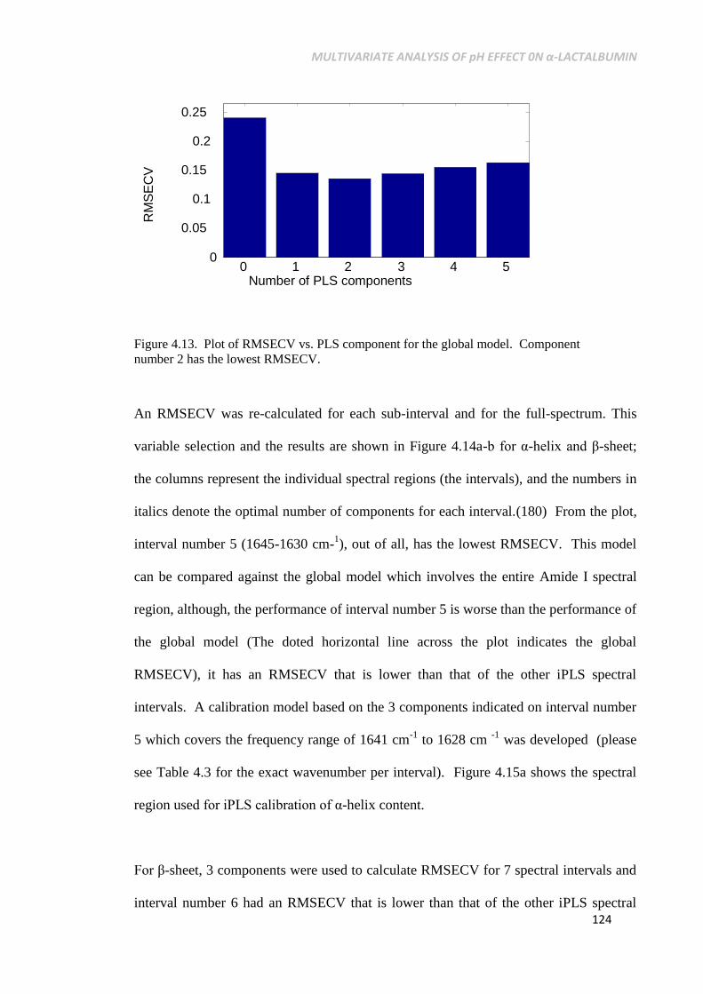
MULTIVARIATE ANALYSIS OF pH EFFECT 0N α-LACTALBUMIN
124
Figure 4.13. Plot of RMSECV vs. PLS component for the global model. Component
number 2 has the lowest RMSECV.
An RMSECV was re-calculated for each sub-interval and for the full-spectrum. This
variable selection and the results are shown in Figure 4.14a-b for α-helix and β-sheet;
the columns represent the individual spectral regions (the intervals), and the numbers in
italics denote the optimal number of components for each interval.(180) From the plot,
interval number 5 (1645-1630 cm-1), out of all, has the lowest RMSECV. This model
can be compared against the global model which involves the entire Amide I spectral
region, although, the performance of interval number 5 is worse than the performance of
the global model (The doted horizontal line across the plot indicates the global
RMSECV), it has an RMSECV that is lower than that of the other iPLS spectral
intervals. A calibration model based on the 3 components indicated on interval number
5 which covers the frequency range of 1641 cm-1
to 1628 cm -1
was developed (please
see Table 4.3 for the exact wavenumber per interval). Figure 4.15a shows the spectral
region used for iPLS calibration of α-helix content.
For β-sheet, 3 components were used to calculate RMSECV for 7 spectral intervals and
interval number 6 had an RMSECV that is lower than that of the other iPLS spectral
0 1 2 3 4 5 0
0.05
0.1
0.15
0.2
0.25
Number of PLS components
RM
SE
CV

USING REGRESSION ANALYSES FOR THE DETERMINATION
OF PROTEIN STRUCTURE FROM FTIR SPECTRA 125
intervals and also lower than the RMSECV of the global model. A calibration model
based on the 3 components indicated on interval number 6 which covers wavenumber
1627 cm-1
to 1614 cm-1
was developed. This β-sheet spectral region deviates from β-
sheet spectral assignment reported by other literatures. Figure 4.15b depicts the spectral
region used for iPLS calibration of α-helix.
Figure 4.14a Each bar in the plot is a spectral interval. The plot shows interval numbers
1-7 ; Interval number 5 corresponds to frequency factors in the range 1641 cm-1
– 1628
cm-1
for α-helix, The dotted line represents the RMSECV for the global iPLS model.
Numbers in italics in each interval bar signifies the number of iPLS components used in
fitting each local model. See Table 4.3 for intervals and wavenumber range. The curve in
the background is a spectrum of the Amide I region.
1 2 3 4 5 6 70
0.05
0.1
0.15
0.2
RM
SE
CV
iPLS Interval number
1 4 2 3 3 3 1

MULTIVARIATE ANALYSIS OF pH EFFECT 0N α-LACTALBUMIN
126
Figure 4.14b. Plot shows interval number 6 (6th bar) corresponding to frequency factors in
the range 1614–1627 cm-1
for β-sheet. See Table 4.3 for each interval actual beginning and
ending wavenumbers). Dotted line is the RMSECV for the global iPLS model. The dotted
line represents the RMSECV for the global iPLS model. Numbers in italics in each
interval bar signifies the number of iPLS components used in fitting each local model.
The curve in the background is a spectrum of the Amide I region.
Table 4.3. Table of intervals and their corresponding frequencies; interval number 8 which
covers the Amide I region was used for the iPLS global model.
1 2 3 4 5 6 70
0.05
0.1
RM
SE
CV
iPLS Interval number
1 4 2 5 3 3 3
Interval
Start
variable
End
variable
Start
wavenumber
End
wavenumber
Number of
variables
1 1 15 1700 1686 15
2 16 30 1685 1671 15
3 31 45 1670 1656 15
4 46 59 1655 1642 14
5 60 73 1641 1628 14
6 74 87 1627 1614 14
7 88 101 1613 1600 14
8 1 101 1700 1600 101

USING REGRESSION ANALYSES FOR THE DETERMINATION
OF PROTEIN STRUCTURE FROM FTIR SPECTRA 127
Figure 4.15a. Plot of the Amide I normalized spectral region shows the spectral region (in
grey bar) used for iPLS analysis of α-helix structure. . The grey bar contains the most
variation for of α-helix structure. This region (1641–1628 cm-1
) corresponds to interval
number 5 from Table 4.14a.
Figure 4.15b. Plot of the normalized spectral region of Amide I that contain the most
significant region (in grey bar) for β-sheet structure. The grey bar contains the most
variation for β-sheet structure. This region (1627 cm-1
–1614 cm-1
) was assigned to
interval number 6 from Figure 4.14b.
1600 1620 1640 1660 1680 17000
0.2
0.4
0.6
0.8
1
Norm
alized inte
nsitie
s
Wavenumber cm-1
1600 1620 1640 1660 1680 17000
0.2
0.4
0.6
0.8
1
Wavemumber cm-1
No
rma
lize
d in
ten
sitie
s

MULTIVARIATE ANALYSIS OF pH EFFECT 0N α-LACTALBUMIN
128
4.6 Results and Discussion
The α-helix and β-sheet secondary structural motifs of proteins have well defined
hydrogen bonding properties which makes them relatively compact and, as a result,
these structures are better defined than other looser spatial structural arrangements such
as turns and coils.(157) This is very evident in the iPLS results obtained from this
work. The selected intervals for all the structural motifs used in this method gave better
prediction over all other intervals that were tried out.
α-helix 4.6.1
Figure 4.16a shows the global prediction fraction of α-helix from the Amide I region vs.
the X-ray diffraction-derived reference fraction for the same structure. The RMSECV
of 0.144 is a little better than that of the traditional PLS model with RMSECV of 0.181
but the iPLS R2 for cross-validation (0.80) is lower than the value for 0.85 found for the
traditional PLS. This difference is not so dramatic to be a deciding factor for which
method to use. The RMSECV figure could have been higher because the model was fit
with 4 components while iPLS model was fit with 3 components.
For each prediction of secondary structure content produced for these intervals, the
factors used to assess the prediction accuracy, were based on the iPLS prediction vs. the
reference X-ray derived PDB data for the secondary structure. The plot in Figure 4.16b
shows the ‘line of fit’ for α-helix from the interval number 5 model (1641 -1628 cm-1)
with 3 latent variables (components). This model gave a RMSECV of 0.149 and an R2
of 0.78 which is below the performance of the global model. Finding a way to divide a
matrix of spectra to give optimal iPLS results is a daunting tasks and required lots of

USING REGRESSION ANALYSES FOR THE DETERMINATION
OF PROTEIN STRUCTURE FROM FTIR SPECTRA 129
trials; sometimes two intervals may need to be merged into one to get accurate results
from the structural analysis.
Figure 4.16a. Prediction line of fit for α-helix from the iPLS global model in the in Amide
I region (1700 – 1600 cm-1
). 3 iPLS components were used for building the model. The
numbers in the plot represent the different proteins in the dataset which are listed in Table
4.4
Figure 4.16b. Prediction line of fit for α-helix from the iPLS local model in the in Amide I
region (1641 cm-1
– 1628 cm-1
). 3 PLS components were used for building the model. The
numbers in the plot are the different proteins in the dataset which are named in Table 4.4.
0 0.2 0.4 0.6 0.8
0
0.2
0.4
0.6
0.8
1
2
3
4
5
6
7
8
9
10
11
12
13
14
15
16
17
18
19
20
21
22
23
24
25
26
27
28
29
3031
32
33
34
35
36
37
38
39
40
41
42
43
44
45
46
47
48
49
50
51
52
53
54
55
56
57
58
59
60
Experimental (X-ray Crystallography: -helix)
Pre
dic
ted (
FT
IR/ iP
LS
)
R2 = 0.8026
RMSECV = 0.1442
0 0.2 0.4 0.6 0.80
0.2
0.4
0.6
0.8
1
2 3
4
5
6
7
8
9
10
11
12
1314
15
16
17
1819
20
21
22
23
24
25
26
27
28
2930
31
32
33
34
35
3637
38
39
40
41
42
43
44
45
46
47
48
49
50
51
52
53
54
55
56
57
58
59
60
Experimental (X-ray Crystallography: -helix)
Pre
dic
ted (
FT
IR/iP
LS
)
RMSECV = 0.1495R
2 = 0.7823

MULTIVARIATE ANALYSIS OF pH EFFECT 0N α-LACTALBUMIN
130
β-sheet 4.6.2
Figure 4.17a shows the global iPLS model plot for the prediction fraction of β-sheet for
the Amide I region vs. X-ray reference fraction from the PDB for the same structure.
The RMSECV for this global model is 0.092 with an R2 of 0.81 while the RMSECV
from the traditional PLS model for β-sheet was 0.050 with R2 of 0.94. The global iPLS
model for β-sheet did much more poorly than the traditional PLS model but this could
be due to the number of components used for iPLS global for Amide I (3 vs. 9
components for traditional PLS). The plot in Figure 4.17b shows the ‘Line of Fit’ for
β-sheet from the model of interval number 6 (1627 -1614 cm-1) with 3 latent variables
(components). This model gave a RMSECV of 0.087 and an R2 of 0.83 which is much
better than the performance of the iPLS global model. Again, this could also be due to
the number of components, 3, used for both local model with 14 variables and global
model with 101 variables; see Table 4.3.
Figure 4.17a. Prediction line of fit for β-sheet from the iPLS global model in the Amide I
region (1700 cm-1
– 1600 cm-1
). 3 iPLS components were used for building the model. The
numbers in the plot are the different proteins in the dataset which are named in Table 4.4.
0 0.1 0.2 0.3 0.4 0.5 0.60
0.1
0.2
0.3
0.4
0.5
0.6
1
2
3
4
5
6
7
8
9
1011
12
13
14
15
16
17
18
19
20
21
22
23
24
25
26
27
28
29
3031
32
33
34
35
36
37
38
39
40
41
42
43
44 45
46
47
48
4950
51
52 53
54
55
56
57
58
59
60
R2 = 0.8052
RMSECV = 0.0924
Experimental (X-ray Crystallography: -sheet)
Pre
dic
ted (
FT
IR/iP
LS
)

USING REGRESSION ANALYSES FOR THE DETERMINATION
OF PROTEIN STRUCTURE FROM FTIR SPECTRA 131
Figure 4.17b. Prediction line of fit for β-sheet from the iPLS local model in the Amide I
region (1627 cm-1
– 1614 cm-1
). 3 iPLS components were used for building the model
from the 6th spectral interval. The numbers in the plot are the different proteins in the
dataset which are named in Table 4.4.
4.7 Validation Set
The Kennard Stone algorithm was used for the splitting of the protein samples into
Training and Test sets. Although the number of proteins in the independent test set were
the same for both PLS and iPLS, a few factors were different between them. The
proteins in the training set for both methods were not completely identical, several
proteins in the calibration set of the PLS method were in the test set of the iPLS method
This is because for iPLS, data selection for calibration set and test set were based on
intervals, regions of the spectra, instead of the full spectra. The number of components
used for the prediction test set models was based on the error of the cross-validation
performed for calibration models. The results of the iPLS validation of 44 proteins in
the test set were as good as the results of the traditional PLS validation result which is
very promising for iPLS method. This comparison is shown in Table 4.5. Figure 4.15a
shows that the model for α-helix fits the data and the Root mean Square Error for
Prediction (RMSEP) is 0.134 with an R2 of 0.78. The β-sheet model also fits the data
0 0.1 0.2 0.3 0.4 0.5 0.6 0.7
0
0.1
0.2
0.3
0.4
0.5
0.6
0.7
1
2
3
4
5
6
7
8
9
10
11
12
13
14
15
1617
18
19
20
21
22
23
24
25
26
27
28
2930
31
32
33
34
35
36
37
38
39
4041
42
43
44
4546
47
48
49
50
5152
53
54
55
56
57
58
59
60
Experimental (X-ray Crystallography: -heet)
Pre
dic
ted (
FT
IR/iP
LS
)
R2 = 0.8281
RMSECV = 0.0868

MULTIVARIATE ANALYSIS OF pH EFFECT 0N α-LACTALBUMIN
132
well with an RMSEP value of 0.089 and an R2 of 0.79. These results are comparable to
the traditional PLS results. To view the PLS calibration results, cross-validation results,
and independent set validation results, see table 4.2a and 4.2b.
Figure 4.18a. Plot of local model line of fit for the prediction of α-helix in Amide I (1641
cm-1
– 1628 cm-1
). 3 PLS components for the 5th spectral interval were used for the
prediction of proteins in the test set.. The numbers in the plot are the different proteins in
the dataset which are named in Table 4.4
Figure 4.18b. Plot of local model line of fit for the prediction of β-sheet in Amide I (1627
cm-1
– 1614 cm-1
). 3 PLS components for the 6th spectral interval were used for the
prediction of proteins in the test set. The numbers in the plot are the different proteins in
the dataset which are named in Table 4.4.
0 0.1 0.2 0.3 0.4 0.5 0.6 0.7 0.8 0.90
0.1
0.2
0.3
0.4
0.5
0.6
0.7
0.8
0.9
1
2
3
4
5
6
7
8
9
10
11
12
13
14
15
16
17
18
19
20
21
22
23
24
2526
27 28
29
3031
32 3334
35
36
37
3839
40
41
42
43
44 45
Experimental (X-ray Crystallography: -heet)
Pre
dic
ted (
FT
IR/iP
LS
)
R2 = 0.7893
RMSEP = 0.1349
0 0.1 0.2 0.3 0.4 0.5
0
0.1
0.2
0.3
0.4
0.5
1 2
3
4
5
6
7
8
9
10
11
1213
14
15
16
17
18
19
20
21
22
23
24 25
26
27
28
29
30 31
32
33
34
35
36
37
38
39
40
41
42
43
4445
R2 = 0.7927
RMSEP = 0.0894
Pre
dic
ted (
FT
IR/iP
LS
)
Experimental (X-ray Crystallography: -sheet)

USING REGRESSION ANALYSES FOR THE DETERMINATION
OF PROTEIN STRUCTURE FROM FTIR SPECTRA 133
Table 4.4. The list of proteins used for the both calibration and test set in the iPLS. These
proteins are listed to match the numbers in the line of fit plot for both calibration and
validation for iPLS models.
Table A2 in Appendix A lists the full name and source (organism) of these proteins”
Num Proteins in Calibration Set Num Proteins in Test Set
1 annexinV 31 esterase(r.oryzae) 1 pyruvate 23 lectin
2 elastin 32 calmodulin 2 transketalose 24 lipase (wheat)
3 porin 33 fibrinogen 3 carbonic anhydrase 25 fetuin
4 trypsin 34 typsin-chymotrypsin 4 pepsin 26 IgG (bovine)
5 alpha-1-antitrypsin 35 invertase 5 alcohol-dehydrog 27 trypsin(hog)
6 myoglobulin 36 IgG (human) 6 reaction centere R. Sphae. 28 apha-Crystallin
7 avidin 37 lipase(c.rugosa) 7 thaumactin 29 superoxide-dismutase
8 phosvitin 38 albumin (bovine) 8 lysozyme (chicken egg) 30 esterase(b.substilis)
9 proteinase 39 d_amino acid dehydr 9 ovalbumin 31 nt-anti-chymotryp
10 tryptophan synthase 40 pyruvate 10 melittin 32 native-anti-thrombin
11 alpha casein 41 transketalose 11 alpha_lactalbumin 33 lactic dehydrog
12 hexakinase 42 carbonic anhydrase 12 staphylokinase-B 34 split-c1 inhibitor
13 l-lactic dehydrogenase 43 pepsin 13 choline oxidase 35 rhodopsin bleached
14 alpha amylase_type2 44 alcohol-dehydrog 14 ribonuclease B 36 split-anti-chymotryp
15 insulin 45 reaction centere R. Sphae. 15 albumin (human) 37 conalbumin
16 chymotrypsin 46 thaumactin 16 trypsin (bovine) 38 anti-thrombin
17 sact1 DIFF 47 lysozyme (chicken egg) 17 ferritin 39 ribonuclease A
18 subtilisin 48 ovalbumin 18 peroxidase 40 trypsinogen
19 rhodopsin unbleached 49 melittin 19 galactose 41 albumin (sheep)
20 phtosystem II 50 alpha_lactalbumin 20 glucose oxidase 42 collagen
21 concanavalin 51 staphylokinase-B 21 hemoglobin 43 split-ovalbumin
22 l-glutathion 52 choline oxidase 22 cytochrome 44 native-c1 inhibitor
23 aprotinin 53 ribonuclease B
24 purple membrane 54 albumin (human)
25 β-lactoglobulin 55 trypsin (bovine)
26 ubiquitin 56 ferritin
27 pig citrate synthase 57 peroxidase
28 ribonuclease S 58 galactose
29 urease 59 glucose oxidase
30 papain 60 hemoglobin
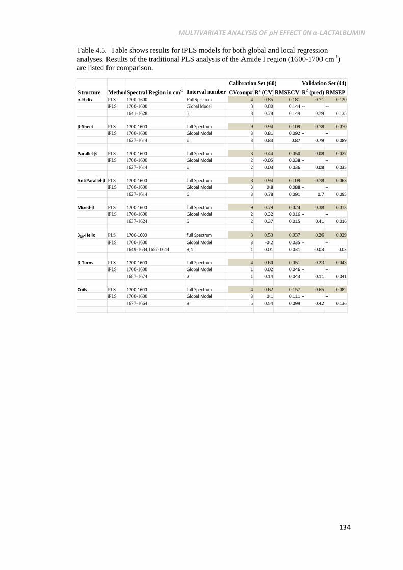
MULTIVARIATE ANALYSIS OF pH EFFECT 0N α-LACTALBUMIN
134
Table 4.5. Table shows results for iPLS models for both global and local regression
analyses. Results of the traditional PLS analysis of the Amide I region (1600-1700 cm-1
)
are listed for comparison.
Calibration Set (60) Validation Set (44)
Structure MethodSpectral Region in cm-1 Interval number CVcomp# R
2 (CV) RMSECV R
2 (pred) RMSEP
α-Helix PLS 1700-1600 Full Spectrum 4 0.85 0.181 0.71 0.120
iPLS 1700-1600 Global Model 3 0.80 0.144 -- --
1641-1628 5 3 0.78 0.149 0.79 0.135
β-Sheet PLS 1700-1600 full Spectrum 9 0.94 0.109 0.78 0.070
iPLS 1700-1600 Global Model 3 0.81 0.092 -- --
1627-1614 6 3 0.83 0.87 0.79 0.089
Parallel-β PLS 1700-1600 full Spectrum 3 0.44 0.050 -0.08 0.027
iPLS 1700-1600 Global Model 2 -0.05 0.038 -- --
1627-1614 6 2 0.03 0.036 0.08 0.035
AntiParallel-β PLS 1700-1600 full Spectrum 8 0.94 0.109 0.78 0.063
iPLS 1700-1600 Global Model 3 0.8 0.088 -- --
1627-1614 6 3 0.78 0.091 0.7 0.095
Mixed-β PLS 1700-1600 full Spectrum 9 0.79 0.024 0.38 0.013
iPLS 1700-1600 Global Model 2 0.32 0.016 -- --
1637-1624 5 2 0.37 0.015 0.41 0.016
310-Helix PLS 1700-1600 full Spectrum 3 0.53 0.037 0.26 0.029
iPLS 1700-1600 Global Model 3 -0.2 0.035 -- --
1649-1634,1657-1644 3,4 1 0.01 0.031 -0.03 0.03
β-Turns PLS 1700-1600 full Spectrum 4 0.60 0.051 0.23 0.043
iPLS 1700-1600 Global Model 1 0.02 0.046 -- --
1687-1674 2 1 0.14 0.043 0.11 0.041
Coils PLS 1700-1600 full Spectrum 4 0.62 0.157 0.65 0.082
iPLS 1700-1600 Global Model 3 0.1 0.111 -- --
1677-1664 3 5 0.54 0.099 0.42 0.136

USING REGRESSION ANALYSES FOR THE DETERMINATION
OF PROTEIN STRUCTURE FROM FTIR SPECTRA 135
4.8 Conclusion
FTIR spectra with PLS gives excellent quantitative results of protein structural analysis.
Tables 4.1a and 4.1b show a good prediction of the proteins structural motifs as
compared to the values given by X-Ray crystallography, for α helix, beta sheets and
other. On the average our regression analyses for the calibration set generated
predictions to within 1-5% accuracy of all secondary structure content (α-helix, β-
sheets, 310-helix, turns and coils) in the Amide I region. The independent test set result
was very good as well. The results obtained for proteins in H2O and D2O were
comparable to the reference data of X-ray crystallography; although in this analysis, the
results (from Table 4.2) of proteins in H2O did slightly better than proteins in D2O.
FTIR absorption spectra contain a great deal of information that can be utilised for
classification and quantitative determination of protein and is a widely applicable
technique; the use of Partial Least Squares (PLS) on FTIR spectra has been
demonstrated as an effective method to provide reliable quantitative structural analysis
of proteins.(157) The Amide II region also gave results comparable to that of the
Amide I region, especially for predictions of helix content; the Amide II region is
known for being less sensitive to secondary structure of protein(181) and some literature
report on the analysis of secondary structure in this region have reported less accurate
results so a good prediction from this region was impressive. Tables 4.1a/b show that
Amide I and II combined gave a much accurate result. In addition to the elucidation of
310-helix which has only being done with linear regression model by Goormaghtigh,
Ruysschaert and Raussens without meaningful result as they clearly stated, (151) we
have also been able to differentiate between parallel and anti-parallel β-sheet, and turns
using our method. This is not always done by spectra analysts because parallel β-sheet
are less common and turns are not so structured and are difficult to determine.
MULTIVARIATE ANALYSIS OF pH EFFECT 0N α-LACTALBUMIN
136
Identifying those critical regions of a spectra for any given secondary structure motif
can improve production cost and reduce analysis time and improve models(182). iPLS
models applied to the local models of Amide I FTIR protein bands showed better
results than the global models for all structural types except in α-helix where the
RMSECV (0.144) of the global model is a little lower than that of the local model
(0.149). Given the number of components used and the lower RMSECV, the results of
iPLS global model came out a little more accurate that of the full-spectrum of traditional
PLS models; however, the RMSEP of full spectrum PLS was much better than the local
model of iPLS for all structural types, meaning that the traditional PLS model did better
as predicting new samples. For quantitative analysis, iPLS is a valuable tool, especially
for the identification of the spectral regions that are more significant for each structural
motif but the trials and errors involved in identifying these intervals coupled with the
fact that the full spectrum PLS analysis does better at quantifying proteins in
independent test set discouraged the further used of the iPLS method for this project.
With iPLS a priori knowledge of spectral regions for each secondary structure may
guide in the spectral variable selection for iPLS; that being said, a look at other
quantitative methods was valuable.
Given the satisfactory performance of Multivariate Analysis tools such as PLS on FTIR
protein spectra, and because of its effectiveness with collinearity,(104) it can be
confirmed that the combination of the two is a powerful tool for the determination of
protein secondary structure from spectra, including the not so common structural types
like 310-helix.
USING REGRESSION ANALYSES FOR THE DETERMINATION
OF PROTEIN STRUCTURE FROM FTIR SPECTRA 137
5 Multivariate analysis of pH effect on α-lactalbumin
5.1 Introduction
In this chapter the developed PLS model for determining the secondary structure of
protein is applied to test the PLS model’s ability to quantitatively determine the
structure of a denatured protein. Bovine -lactalbumin is the protein of choice because
the denatured state of α-lactalbumin (α-LA) is the best characterized folding
intermediate of globular proteins and has been studied by different spectroscopic
techniques (183-185), but it does not have a comprehensive report of its percentage
secondary structure at different pH values.
The backbone hydrogen bonds and the side chain hydrophobic interactions are the most
important bonds that make up the proteins’ secondary and tertiary structure;(186) these
structures can be broken by denaturing conditions and proteins typically need to be in
their native conformations to operate properly, therefore the analysis of their secondary
and tertiary structures is important for characterizing protein stability and function.(106)
The structural changes undergone by proteins can affect their stability, e.g. in drug
formulation where these changes could cause protein aggregation and affect drug
efficacy,(187-189) therefore their higher order structure (secondary and tertiary
structures) must be compared to some reference standard.(106, 190) Structural changes
could also be as a result of misfolding of the protein during biogenesis causing loss of
their functions and also diseases such as Alzheimer's disease and systemic
amyloidoses.(191, 192)
It has been established that proteins in their native states carry out specific biological
functions; understanding what distinguishes a protein’s partially folded states from the
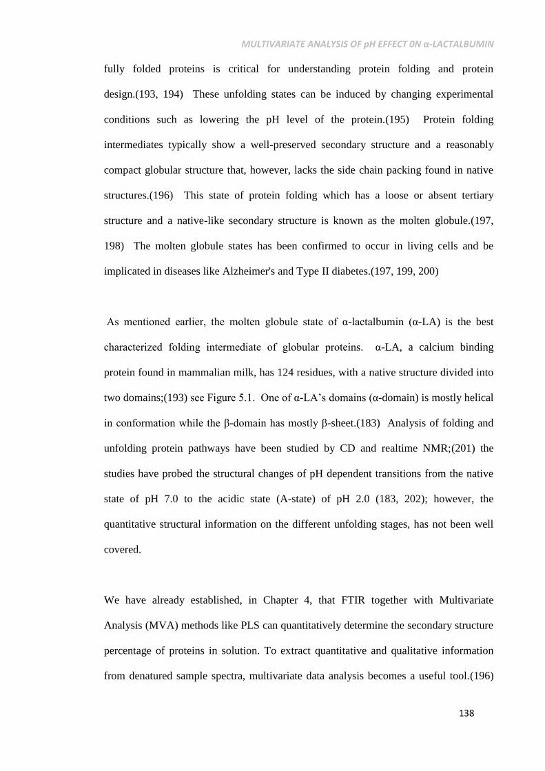
MULTIVARIATE ANALYSIS OF pH EFFECT 0N α-LACTALBUMIN
138
fully folded proteins is critical for understanding protein folding and protein
design.(193, 194) These unfolding states can be induced by changing experimental
conditions such as lowering the pH level of the protein.(195) Protein folding
intermediates typically show a well-preserved secondary structure and a reasonably
compact globular structure that, however, lacks the side chain packing found in native
structures.(196) This state of protein folding which has a loose or absent tertiary
structure and a native-like secondary structure is known as the molten globule.(197,
198) The molten globule states has been confirmed to occur in living cells and be
implicated in diseases like Alzheimer's and Type II diabetes.(197, 199, 200)
As mentioned earlier, the molten globule state of α-lactalbumin (α-LA) is the best
characterized folding intermediate of globular proteins. α-LA, a calcium binding
protein found in mammalian milk, has 124 residues, with a native structure divided into
two domains;(193) see Figure 5.1. One of α-LA’s domains (α-domain) is mostly helical
in conformation while the β-domain has mostly β-sheet.(183) Analysis of folding and
unfolding protein pathways have been studied by CD and realtime NMR;(201) the
studies have probed the structural changes of pH dependent transitions from the native
state of pH 7.0 to the acidic state (A-state) of pH 2.0 (183, 202); however, the
quantitative structural information on the different unfolding stages, has not been well
covered.
We have already established, in Chapter 4, that FTIR together with Multivariate
Analysis (MVA) methods like PLS can quantitatively determine the secondary structure
percentage of proteins in solution. To extract quantitative and qualitative information
from denatured sample spectra, multivariate data analysis becomes a useful tool.(196)

USING REGRESSION ANALYSES FOR THE DETERMINATION
OF PROTEIN STRUCTURE FROM FTIR SPECTRA 139
In this chapter, MVA methods like Partial Least Squares (PLS) and Principal
Component Analysis (PCA) are applied to bovine α-lactalbumin, to characterize the
secondary structure conformational changes at each unfolding transition as a function of
pH. It has been reported by Troullier et al.(201) that FTIR can differentiate between
native and non-native secondary structure present in folding states. We will investigate
and compare the secondary structure results at both the native and non-native states of
samples of -LA measured with FTIR spectroscopy.
Figure 5.1. The diagram on the left of α-LA (PDB ID: 1HFZ) shows the native structure of
α-LA, the intermediate unfolded state is shown in the middle and the unfolded state is
represented on the right. The PDB reported structure of the bovine α-LA (1HFZ is 43%
helical structure, 9% -sheet, 48% other. The Ca2+
ions are shown in black, the blue ribbon
represents α-helix, the green ribbon represents 310-helix and the green arrows represent β-
sheet
5.2 Sample preparation
Bovine α-La was bought from Sigma-Aldrich, and was used without further
purification. Solutions of 50 mg/mL of α-La were prepared in deionized H2O; as
mentioned in D’Antonio, et al.(106)
protein concentrations higher than 25mg/mL
provide great precision in IR spectra. Protein unfolding states can be generated by
modification of the experimental conditions, by changing pH, temperature or
pressure.(203, 204) In this experiment, pH levels were adjusted with diluted HCl acid
to induce conformational changes between pH 2.0 and 7.0. Lowering the pH level by

MULTIVARIATE ANALYSIS OF pH EFFECT 0N α-LACTALBUMIN
140
~0.5 pH units for every new preparation of α-LA solution gave a total of eleven α-LA
samples.
5.3 ATR-FTIR Spectroscopy
All sample spectra were acquired with ATR-FTIR at 32 scans and a resolution of 4 cm-1
for both background and sample measurement; this is described in Chapter 2 for sample
measurements. The overlapping bands in the Amide I region were subjected to second
derivative analysis using a Savistzky-Golay algorithm with 5 degrees; this reveals the
underlying absorption changes.(201) Second derivatives were also calculated for the
Amide II and Amide III regions to provide a consistent basis for analysis.
5.4 PLS and PCA Modelling Technique
The second derivative spectra of all 11 α-LA samples in the Amide I, Amide II and
Amide III regions of the spectra were fed into the PLS application; the 11 α-LA samples
were used as an independent test set; the calibration set of 75 spectra covering Amide I,
II and III regions were extracted from the database used in Chapters 3 and 4. For data
processing, in-house Matlab (R2013a) routine of PLS and PCA codes were developed.
An internal validation (cross-validation) was done on all spectra and the number of
latent variables chosen from cross-validation was used for the prediction set. The
spectral plot of Figure 5.2 shows unfolded stages of α-LA (arising from changes in the
pH levels) in the Amide I, Amide II and Amide III regions for each spectrum. The
unfolding of the protein structure can be monitored through changes in the frequencies
and intensities of the well-resolved peaks in the FTIR spectra (205)
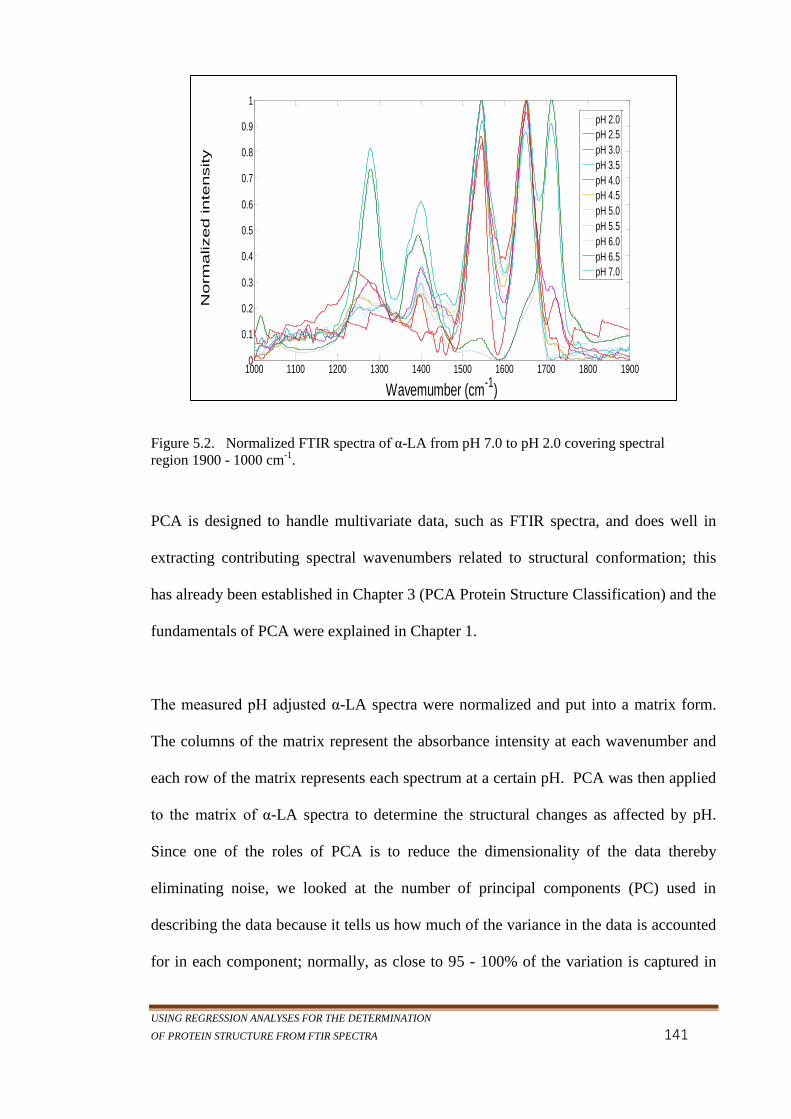
USING REGRESSION ANALYSES FOR THE DETERMINATION
OF PROTEIN STRUCTURE FROM FTIR SPECTRA 141
Figure 5.2. Normalized FTIR spectra of α-LA from pH 7.0 to pH 2.0 covering spectral
region 1900 - 1000 cm-1
.
PCA is designed to handle multivariate data, such as FTIR spectra, and does well in
extracting contributing spectral wavenumbers related to structural conformation; this
has already been established in Chapter 3 (PCA Protein Structure Classification) and the
fundamentals of PCA were explained in Chapter 1.
The measured pH adjusted α-LA spectra were normalized and put into a matrix form.
The columns of the matrix represent the absorbance intensity at each wavenumber and
each row of the matrix represents each spectrum at a certain pH. PCA was then applied
to the matrix of α-LA spectra to determine the structural changes as affected by pH.
Since one of the roles of PCA is to reduce the dimensionality of the data thereby
eliminating noise, we looked at the number of principal components (PC) used in
describing the data because it tells us how much of the variance in the data is accounted
for in each component; normally, as close to 95 - 100% of the variation is captured in
1000 1100 1200 1300 1400 1500 1600 1700 1800 19000
0.1
0.2
0.3
0.4
0.5
0.6
0.7
0.8
0.9
1
Wavemumber (cm-1
)
Norm
alized inte
nsity
pH 2.0
pH 2.5
pH 3.0
pH 3.5
pH 4.0
pH 4.5
pH 5.0
pH 5.5
pH 6.0
pH 6.5
pH 7.0

MULTIVARIATE ANALYSIS OF pH EFFECT 0N α-LACTALBUMIN
142
the first four components, of which the first two may hold 80 - 90%.(206) This means
that the information in the data can be studied by looking at the first and second
principal components. We also visualized the plots of the PCA component scores (the
transformed variable values) and the loadings spectra resulting from the Principal
Component as these can help with observing how the samples are related to each other.
5.5 Results and Discussion
Inspection of the Amide I Spectral Plots 5.5.1
A visual inspection of the normalized spectra (Figure 5.3) shows that the spectra of
bovine α-LA at pH 7.0 to 3.5 had the usual Amide I peaks at about 1656 cm-1
. This
peak intensity dropped significantly for pH 3.0 and increased around 1715 cm-1
with the
right shoulder shifted to 1740 cm-1
. This suggests a decrease in the amount of
secondary structure at pH 3.0. For the spectrum of pH 4.0 spectra, there was a shift in
the right shoulder from 1700 cm-1
to 1750 cm-1
and a slight peak was beginning to
develop around 1720 cm-1.
Figure 5.3 The normalized Amide I region of -LA shows the changes and shifts in
spectral peaks as pH decreases from 4.0 to 2.0
1600 1620 1640 1660 1680 1700 1720 1740 1760 1780 18000
0.1
0.2
0.3
0.4
0.5
0.6
0.7
0.8
0.9
1
Wavemumber (cm-1
)
Norm
alized inte
nsity
pH 2.0
pH 2.5
pH 3.0
pH 3.5
pH 4.0
pH 4.5
pH 5.0
pH 5.5
pH 6.0
pH 6.5
pH 7.0

USING REGRESSION ANALYSES FOR THE DETERMINATION
OF PROTEIN STRUCTURE FROM FTIR SPECTRA 143
A shift of the Amide I peak was seen at pH 2.5 and pH 2.0 around 1715 cm-1
. This
visual inspection of the spectra explains the secondary structure quantitative results for
the decrease in β-sheet for pH 3.0 spectra and a big gain in α-helix as at pH 2.5 and pH
2.0. β-sheet picked up as α-helix declined (see section 5.5.2 for quantitative results).
Figures 5.4a/b and 5.5b/c reveals the second derivatives of the spectra of pH 7.0 and pH
2.0 and pH 2.5, and the shift in peaks from 1657 to 1715 cm-1
. The plots clearly
demonstrate that as the pH levels drop, the structure of the protein goes through
changes. The second derivative band at pH 7.0 is much in line with the peak of the
normalized spectrum which has a major contribution for α-helix at 1657 cm-1
and this is
similar to the pronounced band around 1715 cm-1
at pH 2.0. The peak at 1630 cm-1
, a β-
sheet band, is almost non-existent at pH 3.5 and pH 3.0, but becomes more pronounced
at pH 2.0; the PLS analysis results in Table 5.1 reflects this.
Figure 5.4a. Plot of the second derivatives of the FTIR spectrum for α-LA in the native
state at pH 7.0. A peak at 1657-1658 cm-1
is clearly visible. The second derivatives for pH
6.5 and 6.0 (not shown) are very similar.
1600 1620 1640 1660 1680 1700
Wavemumber (cm-1
)
d2A
/dv
2
pH 7.0
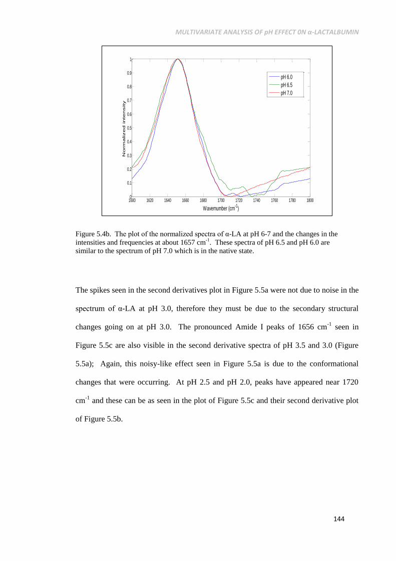
MULTIVARIATE ANALYSIS OF pH EFFECT 0N α-LACTALBUMIN
144
Figure 5.4b. The plot of the normalized spectra of α-LA at pH 6-7 and the changes in the
intensities and frequencies at about 1657 cm-1
. These spectra of pH 6.5 and pH 6.0 are
similar to the spectrum of pH 7.0 which is in the native state.
The spikes seen in the second derivatives plot in Figure 5.5a were not due to noise in the
spectrum of α-LA at pH 3.0, therefore they must be due to the secondary structural
changes going on at pH 3.0. The pronounced Amide I peaks of 1656 cm-1
seen in
Figure 5.5c are also visible in the second derivative spectra of pH 3.5 and 3.0 (Figure
5.5a); Again, this noisy-like effect seen in Figure 5.5a is due to the conformational
changes that were occurring. At pH 2.5 and pH 2.0, peaks have appeared near 1720
cm-1
and these can be as seen in the plot of Figure 5.5c and their second derivative plot
of Figure 5.5b.
1600 1620 1640 1660 1680 1700 1720 1740 1760 1780 18000
0.1
0.2
0.3
0.4
0.5
0.6
0.7
0.8
0.9
1
Wavemumber (cm-1
)
No
rm
alize
d in
ten
sity
pH 6.0
pH 6.5
pH 7.0
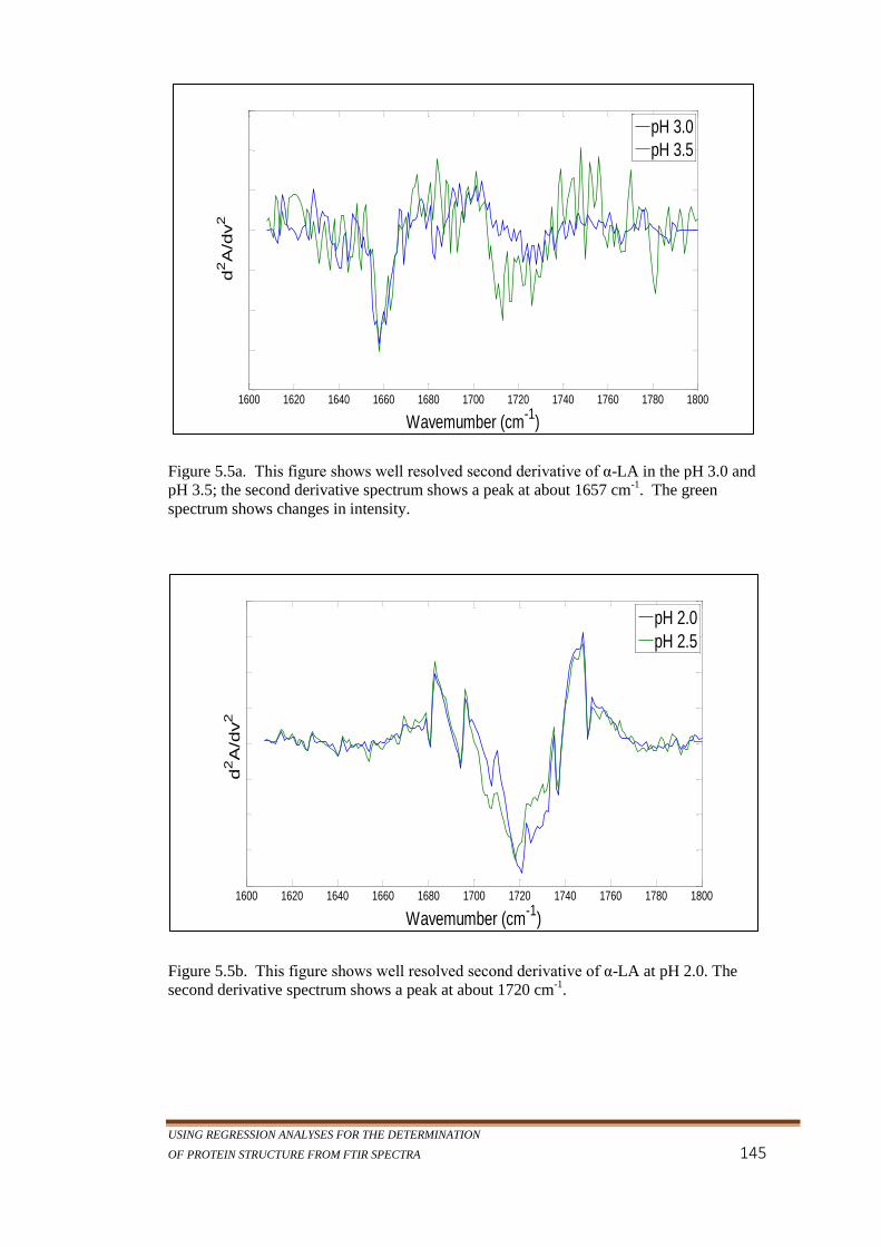
USING REGRESSION ANALYSES FOR THE DETERMINATION
OF PROTEIN STRUCTURE FROM FTIR SPECTRA 145
Figure 5.5a. This figure shows well resolved second derivative of α-LA in the pH 3.0 and
pH 3.5; the second derivative spectrum shows a peak at about 1657 cm-1
. The green
spectrum shows changes in intensity.
Figure 5.5b. This figure shows well resolved second derivative of α-LA at pH 2.0. The
second derivative spectrum shows a peak at about 1720 cm-1
.
1600 1620 1640 1660 1680 1700 1720 1740 1760 1780 1800
Wavemumber (cm-1
)
d2A
/dv
2
pH 3.0
pH 3.5
1600 1620 1640 1660 1680 1700 1720 1740 1760 1780 1800
Wavemumber (cm-1
)
d2A
/dv
2
pH 2.0
pH 2.5

MULTIVARIATE ANALYSIS OF pH EFFECT 0N α-LACTALBUMIN
146
Figure 5.5c. Plot of the normalized spectra of α-LA at pH 2.0-3.5 and the shifts in the
intensities and frequencies.
Amide I PLS Results 5.5.2
We first investigated changes in the Amide I band because this band contains
information on the peptide backbone vibrational frequencies based on their hydrogen
bonding, therefore, the major information on structural changes is contained in this
band.(201) First, the secondary structure of bovine α-LA was assessed by the
comparison of the PLS result of pH 7.0 sample with the native reference values from
DSSP. This had to be done to validate the use of this method in the study of other non-
native states of α-LA. From the values presented in Table 5.1, we can see that structural
values of pH 7.0 (α-helix= 0.37, β-sheet = 0.08, 310-helix = 0.10, Turns = 0.17, 0ther =
0.27).are similar to the reference values of pH 8.0 (α-helix= 0.31, β-sheet = 0.07, 310-
helix = 0.14, Turns = 0.18, 0ther = 0.31). There is about -0.06 difference in α-helix and
1600 1620 1640 1660 1680 1700 1720 1740 1760 1780 18000
0.1
0.2
0.3
0.4
0.5
0.6
0.7
0.8
0.9
1
Wavemumber (cm-1
)
Norm
alized in
tensity
pH 2.0
pH 2.5
pH 3.0
pH 3.5

USING REGRESSION ANALYSES FOR THE DETERMINATION
OF PROTEIN STRUCTURE FROM FTIR SPECTRA 147
-0.01 difference in values of β-sheet from the two different methods (FTIR and X-ray
crystallography). The value differences of 310-helix, turns and ‘other’ between the two
methods are within 0.01 and 0.04; which is remarkable. DSSP script was used to
calculate the secondary structure assignments of α-lactalbumin from the X-ray crystal
3D structure entries in the PDB. However, PDB combines α-helix and 310-helix into
one as helical motif, and as such, PDB helical value for bovine α-LA is 43% helical and
9% for β-sheet. A combination of the α-helix and 310-helix values from the FTIR
results (45%) presented in Table 5.1 is in close agreement with X-ray crystallography
values. This separation of secondary structure values by FTIR spectra cannot be
accurate for other methods like CD because with CD, β-sheet, turns and disordered
structure are hard to separate.(207)
The PLS analysis for the Amide I also shows that the sample for pH 6.5 has a native
structure form (α-helix = 0.34, β-sheet = 0.8, 310-helix = 0.12, Turns = 0.16, Other =
0.32) which is close to the DSSP referenced α-LA structure. In these pH structural
values (pH 7.0 to pH 6.5), there was no visible formation of non-native structures,
compared to the native reference protein.
Given the above results, PLS is applied to the FTIR spectra of α-LA at other pHs. The
PLS results show that there were changes in the structure of α-lactalbumin, as the pH
was lowered. There was an increase in α-helix content for pH 6 through pH 3 (as shown
in Table 5.1), especially at pH 3.0 (α-helix = 0.44, β-sheet = 0.04, 310-helix = 0.15,
Turns = 0.18, Other = 0.25). β-sheet was significantly lower at pH 3.0 and then
increased significantly at pH 2.5 and pH 2.0 while α-helix reduced; a decrease in
disordered structure (Other) was also noticeable seen for pH 3.0; see Table 5.1. It can

MULTIVARIATE ANALYSIS OF pH EFFECT 0N α-LACTALBUMIN
148
also be seen that there was an increase in α-helix and a decrease in β-sheet at pH 5.5 but
not as significant as that at 3.0. Overall, from the Amide I spectra measured in this
study, there were some changes in the α-helix content between pH 6.0 and 3.5 but β-
sheet increased slowly and was lower at pH 3.0 before increasing drastically; this agrees
well with findings of Kim and Baum (184) who stated that the denaturation profile of α-
LA occurred in the pH range of 3.0 to 5.0. The figures remained stable between pH 4.0
and pH 5.0. The proportions of the secondary structure of the analysed α-LA are
presented in Table 5.1 and Figure 5.3. These secondary structural changes at pH 2.5
and pH 2.0 are also evident in Figure 5.5c and in their FTIR spectra of Figure 5.6.
Table 5.1. PLS prediction results for the secondary structure content of Amide I region of
α-lactalbumin at different pH levels using normalized and 2nd
derivative pre-processed
data. Structural values are presented as proportions calculated from 1HFZ (pH 8.0) file
using DSSP script.
Parβ-Sheet denotes parallel -sheet; Anti par β-Sheet denotes anti-parallel -sheet
Amide I
pH α-Helix residueA β-Sheet residueB Par β-Sheet Anti-par β-Sheet Mixed β-Sheet 310-Helix Turns Other
2.0 0.30 0.01 0.15 -0.08 0.01 0.08 0.00 0.14 0.14 0.29
2.5 0.31 0.00 0.13 -0.06 0.01 0.06 0.00 0.14 0.15 0.30
3.0 0.44 -0.13 0.04 0.03 0.02 -0.04 0.00 0.15 0.18 0.25
3.5 0.41 -0.10 0.10 -0.03 0.02 0.09 0.00 0.08 0.15 0.29
4.0 0.38 -0.07 0.10 -0.03 0.02 0.08 0.00 0.09 0.17 0.30
4.5 0.39 -0.08 0.10 -0.03 0.01 0.10 0.00 0.10 0.16 0.28
5.0 0.38 -0.07 0.11 -0.04 0.01 0.10 0.00 0.10 0.16 0.28
5.5 0.42 -0.11 0.07 0.00 0.01 0.06 0.00 0.10 0.17 0.27
6.0 0.41 -0.10 0.08 -0.01 0.01 0.05 0.00 0.09 0.17 0.29
6.5 0.34 -0.03 0.08 -0.01 0.00 0.05 0.00 0.12 0.16 0.32
7.0 0.37 -0.06 0.08 -0.01 0.01 0.08 0.00 0.10 0.17 0.27
DSSP
8.0 0.31 0.07 0.00 0.07 0.00 0.14 0.18 0.31

USING REGRESSION ANALYSES FOR THE DETERMINATION
OF PROTEIN STRUCTURE FROM FTIR SPECTRA 149
Figure 5.6. This plot highlights changes in the secondary structure of α-LA as a function
of pH, based on PLS analysis. The horizontal axis values represents the pH values, the
vertical axis represents the secondary structure proportions. Below pH 3.0, a gain in β-
sheet and a loss in α-helix is seen. The error bars were calculated from the PLS result
residual for each spectrum (which is the observed X-ray value – the calculated FTIR
value).
Inspection of the Amide II Spectral Plots 5.5.3
In the Amide II region we found a main peak of the native form of α-LA at 1546 cm-1
,
as depicted in Figure 5.7, and a peak of the A-state (pH 2.0) at 1521 cm-1
. Although
there appeared to be structural changes in the spectral plot, the change in intensities that
was seen in the Amide I region was not noticed in the Amide II region; however, a shift
in frequencies were noticeable, especially for pH 2.5 and pH 2.0. The spectrum at pH
2.5 developed a noticeable structural change but maintained a peak at 1546 cm-1
.

MULTIVARIATE ANALYSIS OF pH EFFECT 0N α-LACTALBUMIN
150
Figure 5.7. The plot of the normalized spectra of α-LA at pH 2.0 -7.0. Plot shows peak
shift and structural changes especially for pH 2.5 and pH 2.0
Amide II PLS Results 5.5.4
For Amide II results, again the comparison between the PLS result of pH 7.0 and the
known structural values (PDB code 1HFZ) of X-ray crystallography calculated by
DSSP was made to validate this method as fit enough to study other pH ranges in this
region (1480-1575 cm-1
); The secondary structure figures for pH 7.0 (α-helix = 0.36, β-
sheet = 0.10, 310-helix = 0.11, Turns = 0.16, disorder = 0.30), are very similar to the
DSSP values (α-helix = 0.31, β-sheet = 0.07, 310-helix = 0.14, Turns = 0.18, disorder =
0.31) with residues of -0.04 and -0.03 for α-helix and β-sheet respectively. Although
there were structural fluctuations from one pH to another, a noticeable structural
similarity was observed at pH 4.5 (α-helix= 0.45, β-sheet=0.05, 310-helix = 0.11, Turns
= 0.16, Other = 0.25) and at pH 5.0 (α-helix= 0.45, β-sheet = 0.05, 310-sheet = 0.11,
1480 1500 1520 1540 1560 1580 16000
0.2
0.4
0.6
0.8
1
Wavemumber (cm-1
)
Norm
alized inte
nsity
pH 2.0
pH 2.5
pH 3.0
pH 3.5
pH 4.0
pH 4.5
pH 5.0
pH 5.5
pH 6.0
pH 6.5
pH 7.0

USING REGRESSION ANALYSES FOR THE DETERMINATION
OF PROTEIN STRUCTURE FROM FTIR SPECTRA 151
turns = 0.16, disorder = 0.25); a little decrease in disordered structure was also observed
at these pH levels (pH 4.5 and pH 5.0). Again, comparing these values against those for
the known structure from DSSP (α-helix = 0.31, β-sheet = 0.07, 310-helix = 0.14, Turns
= 0.18, disorder = 0.31), we see that α-helix structural values at these pH levels were
0.14 more than the α-helix value of the reference protein. β-sheet value was reduced at
pH 5.0 and pH 4.5 but it increased drastically after pH 3.5, more than doubled in value
at pH 2.0, while a reduction in α-helix was seen at these acidic states. These results are
listed in Table 5.2.
Table 5.2. PLS Prediction results for the secondary structure of Amide II region of α-LA at
different pH levels using normalized and 2nd
derivative pre-processed data. Structural
values are presented in proportions.
Parβ-Sheet denotes parallel beta sheet; Anti par β-Sheet denotes anti-parallel beta-sheet
Inspection of the Amide III Spectral Plots 5.5.5
Denatured protein produced some alteration in the Amide III band of α-Lactalbumin
spectra as shown in Figure 5.8 and Figure 5.9. It can be observed that the peaks of the
Amide II
pH α-Helix β-Sheet Par β-Sheet Anti-par β-Sheet Mixed β-Sheet 310-Helix Turns Other
2.0 0.25 0.06 0.19 -0.12 0.01 0.16 0.00 0.11 0.18 0.32
2.5 0.32 -0.01 0.13 -0.06 0.00 0.12 0.00 0.08 0.16 0.32
3.0 0.40 -0.09 0.10 -0.03 0.02 0.07 0.00 0.08 0.14 0.28
3.5 0.42 -0.11 0.07 0.00 0.02 0.05 0.00 0.09 0.16 0.29
4.0 0.37 -0.06 0.12 -0.05 0.00 0.10 0.01 0.10 0.15 0.27
4.5 0.45 -0.14 0.05 0.02 0.02 0.02 0.00 0.11 0.16 0.25
5.0 0.45 -0.14 0.05 0.02 0.01 0.03 0.00 0.11 0.16 0.25
5.5 0.43 -0.12 0.06 0.01 0.02 0.04 0.00 0.11 0.16 0.26
6.0 0.33 -0.02 0.12 -0.05 0.00 0.10 0.00 0.10 0.14 0.33
6.5 0.26 0.05 0.14 -0.07 0.02 0.13 0.01 0.12 0.13 0.32
7.0 0.36 -0.05 0.10 -0.03 0.01 0.08 0.01 0.11 0.16 0.30
DSSP
8.0 0.31 0.07 0.00 0.07 0.00 0.14 0.18 0.31

MULTIVARIATE ANALYSIS OF pH EFFECT 0N α-LACTALBUMIN
152
spectra of pH 3.4 through pH 2.0 registered at 1278 cm-1
but pH 3.5 and pH 3.0 were
beginning to show alterations at the shoulders. These settled changes were picked up by
the PLS quantitative result in Table 5.3 for α-helix and β-sheet. Amide III bands at
1300, 1260, and 1235 cm-1
regions have been assigned to α-helix, disordered, and β-
sheet structures.(208). The 1250 cm-1
band normally seen for Amide III peak appeared
at 1278 cm-1
; This means that the pH dependent structural changes are not local to the
Amide I region alone but are also effective in the Amide III region These peak values
changes at about the same regions in the Amide III have also been reported by Anderle
and Meldelsohn(209) in their work for denatured proteins.
Figure 5.8. This is the plot of the effect of pH 3.5 (intermediate) – pH 2.0 on the
normalized Amide I spectral region of α-LA protein. Plot shows slight changes at these pH
levels. The different spectral colours represent different pH levels.
Amide III bands for pH 4.0 – pH 5.5 had their main peak at 1250 cm-1
. In addition to
the major peak at 1250 cm-1
which correlates to the β-sheet region of Amide III, pH 5.0
and pH 5.5 had reduced intensities but significant peaks at 1290 cm-1
and 1300 cm-1
1200 1250 1300 13500
0.2
0.4
0.6
0.8
1
Wavemumber (cm-1
)
Norm
alized inte
nsity
pH 2.0
pH 2.5
pH 3.0
pH 3.5

USING REGRESSION ANALYSES FOR THE DETERMINATION
OF PROTEIN STRUCTURE FROM FTIR SPECTRA 153
respectively (β-turns); these regions are in agreement with the α-helix regions for
Amide III (α-helix: 1330–1295 cm−1
, β-sheets: 1250–1220 cm−1
, β-turns: 1295–1270
cm−1
, random coils: 1270–1250 cm−1
) reported by Cai and Singh(39) in their study of
infrared bands for secondary structure. The spectra for these pHs were not as smooth as
that of the spectra of the native state α-LA (pH 7.0); this is because of the many spectral
features present in the Amide III region.
Figure 5.9. Plot of Amide III region depicts peaks shift for pH 5.5 - pH 4.0 at 1250 cm-1
and pH 4.0 at 1279 cm-1
respectively.
At pH 7.0 and 6.5, the spectral peak was at 1256 cm-1
as shown by the plot of Figure
5.10 and well in agreement with literature report for the Amide III region peak(210). At
pH 6.0 a peak had developed at 1240 cm-1
and this make the transition to the 1250 peak
seen at pH 5.5. Amide III PLS results obtained in this experiment are close to X-ray
crystallography values for α-lactalbumin.
1200 1250 1300 13500
0.1
0.2
0.3
0.4
0.5
0.6
0.7
0.8
0.9
1
Wavemumber (cm-1
)
Norm
alized inte
nsity
pH 4.0
pH 4.5
pH 5.0
pH 5.5

MULTIVARIATE ANALYSIS OF pH EFFECT 0N α-LACTALBUMIN
154
Figure 5.10. Plot of Amide III region depicts peak for pH 7.0 (native protein) at 1256 cm-1
Amide III PLS Results 5.5.6
Amide I and Amide II regions of FTIR spectra are the two regions popularly used in the
determination of protein secondary structure. The Amide III region (1200-1350 cm-1
) is
often neglected due to its relative weakness, yet this region offers some advantages for
the IR study because the range of vibrational frequency for secondary structure in the
Amide III region is somewhat greater than Amide I or Amide II.(209) Moreover, the
water vapour absorption overlap found in the Amide I region is not an issue in the
Amide III region. PLS results of native and unfolding spectra in this study are
highlighted in Table 5.3. At pH 7.0 , pH 6.5 and especially at pH 6.0, the value of α-
helix increased as compared to its DSSP numbers (See Table 5.3) -sheet increased
tremendously at pH 5.0, 3.0, 2.5 and pH 2.0 while α-helix for these pH values reduced
from the values seen at pH 6.0, pH 6.5 and pH 7.0. sheet contributions decreased at
pH 4.0 and pH 3.5; an increase in β-sheet formation was seen as the pH reached the A-
state (2.0). The spectra of pH 7.0 has the closest values to that of the reference protein,
1200 1250 1300 13500
0.1
0.2
0.3
0.4
0.5
0.6
0.7
0.8
0.9
1
Wavemumber cm-1
Norm
alized inte
nsity
pH 6.0
pH 6.5
pH 7.0
pH 6.0
pH 6.5
pH 7.0

USING REGRESSION ANALYSES FOR THE DETERMINATION
OF PROTEIN STRUCTURE FROM FTIR SPECTRA 155
showing that it is possible to determine the secondary structures of proteins from the
Amide III region of the native protein spectrum (see Table 5.3).
Table 5.3. PLS Prediction results for the secondary structure content of Amide III region of
α -lactalbumin at different pH levels using normalized and 2nd
derivative pre-processed
data. Structural values are presented in proportions.
Parβ-Sheet denotes parallel beta sheet; Anti par β-Sheet denotes anti-parallel beta-sheet
PCA of α-Lactalbumin Spectra 5.5.7
PCA did well in describing the changes in the secondary structure of the α-LA
unfolding process; this PCA analysis was performed on Amide through Amide III. PC1
captured close to 95% of the total Amide I absorbance and the PC2 component captures
about 5%, while PC3 captured 3% of the remaining variances not described by the PC1
and PC2. This means that the variation in the data are well distributed and data noise
distortion was not an issue.
The Principal Component Score plot of Figure 5.11 shows the classification of -LA
spectra based on its pH levels. From this plot it can be seen that between pH 7.0 and pH
4.5, α-LA is close to its native structure as depicted on the left of PC1, while the acidic
lower pH structures lie on the right of the plot. PC2 places the spectra with the most
Amide III
pH α-Helix β-Sheet Par β-Sheet Anti-par β-Sheet Mixed β-Sheet 310-Helix Turns Other
2.0 0.34 0.19 0.03 0.15 0.00 0.09 0.13 0.29
2.5 0.34 0.19 0.03 0.15 0.00 0.09 0.14 0.29
3.0 0.23 0.23 0.00 0.21 0.00 0.09 0.12 0.32
3.5 0.36 0.18 0.02 0.15 0.00 0.10 0.14 0.29
4.0 0.36 0.15 0.00 0.13 0.01 0.14 0.16 0.30
4.5 0.28 0.17 0.00 0.17 0.00 0.10 0.16 0.31
5.0 0.25 0.20 0.02 0.17 0.00 0.09 0.16 0.28
5.5 0.34 0.12 0.01 0.12 0.01 0.13 0.18 0.24
6.0 0.54 -0.11 -0.01 -0.02 -0.01 0.13 0.21 0.17
6.5 0.48 0.06 -0.02 0.07 -0.01 0.13 0.18 0.20
7.0 0.40 0.08 0.01 0.08 0.01 0.14 0.17 0.26
DSSP
8.0 0.31 0.07 0.00 0.07 0.00 0.14 0.18 0.31

MULTIVARIATE ANALYSIS OF pH EFFECT 0N α-LACTALBUMIN
156
structural shifts at the top (pH 4.0 to pH 3.0). The score plot shows a gradual structural
shift from 5.5 to 4.5 and then a fast shift to pH 3.5, pH 3.0 and pH 2.5 before slowing
down; this suggests a conformational change in the process of unfolding.(211) This
also supports the Amide I stable intermediate figure obtained from PLS for pH 5.0
through pH 4.0 (see Table 5.1). A clear 3 state transition can be seen in the PCA score
plot of Figure 5.13, the native (N) state on the left of PC1, the unfolded stable (U) state
on the right of PC1 and the intermediate (I) state at the top clearly separated by PC2.
Figure 5.11. Score plot of α-LA at different pH on the first and second principal
components. Principal Component Score plot shows the classification of α-LA spectra
based on the pH levels. PC1 has more native state spectra on left and acidic state spectra on
the right. PC2 separates the intermediates at the top
The loadings plot presented in Figure 5.12 and Figure 5.13 enabled us to classify the
absorbance changes into ranges attributed to the three states. Using the PCA approach,
it was possible to detect the changes that are directly correlated with the Amide I,
Amide II and Amide III regions of the FTIR spectra.(212) These are indicated in the
three positive PC1 peaks around 1656 cm-1
1545 cm-1
and 1280 cm-1
respectively. The
-15 -10 -5 0 5 10 15 20 25 30 35-6
-4
-2
0
2
4
6
8
First Principal Component
Se
co
nd
Prin
cip
al C
om
po
ne
nt
pH 2.0pH 2.5
pH 3.0pH 3.5
pH 4.0
pH 4.5
pH 5.5
pH 7.0
pH 5.0pH 6.5
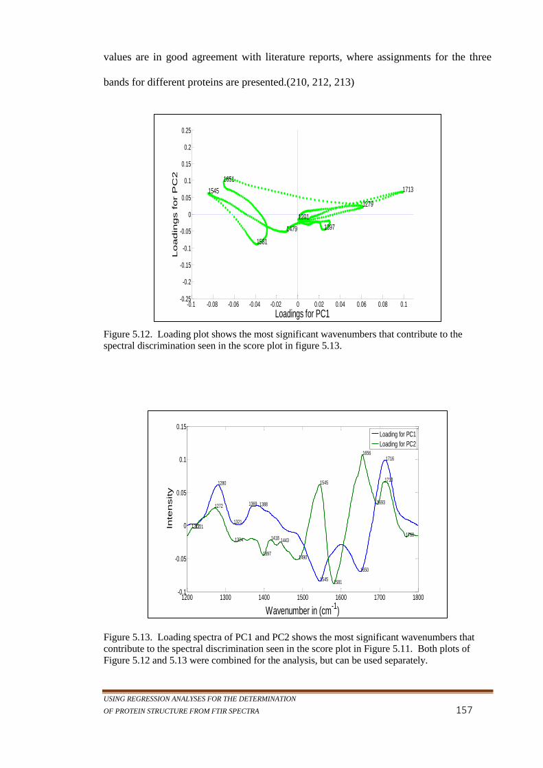
USING REGRESSION ANALYSES FOR THE DETERMINATION
OF PROTEIN STRUCTURE FROM FTIR SPECTRA 157
values are in good agreement with literature reports, where assignments for the three
bands for different proteins are presented.(210, 212, 213)
Figure 5.12. Loading plot shows the most significant wavenumbers that contribute to the
spectral discrimination seen in the score plot in figure 5.13.
Figure 5.13. Loading spectra of PC1 and PC2 shows the most significant wavenumbers that
contribute to the spectral discrimination seen in the score plot in Figure 5.11. Both plots of
Figure 5.12 and 5.13 were combined for the analysis, but can be used separately.
-0.1 -0.08 -0.06 -0.04 -0.02 0 0.02 0.04 0.06 0.08 0.1-0.25
-0.2
-0.15
-0.1
-0.05
0
0.05
0.1
0.15
0.2
0.25
Loadings for PC1
Loadin
gs for P
C2
1545
1581
1713
1279
13971479
1651
1201
1200 1300 1400 1500 1600 1700 1800-0.1
-0.05
0
0.05
0.1
0.15
Wavenumber in (cm-1
)
Inte
nsity
16561716
1713
1693
1650
15811545
1545
14901397
1280
1272
12211321
1324
1369
1418 1443
1388
1768
1212
Loading for PC1
Loading for PC2

MULTIVARIATE ANALYSIS OF pH EFFECT 0N α-LACTALBUMIN
158
As can be seen in Figure 5.15, PC1 depicted 1651 cm-1
from the Amide 1 region and
1546 cm-1
from the Amide II region as significant marker bands on the negative
intensities; these marker bands contribute strongly to pH 7.0 down to 4.0; 1713 cm-1
on
the positive side is significant to pH 3.0 through to pH 2.0; PC2 has also picked up these
bands as 1656 cm-1
for Amide I, 1546 cm-1
for Amide II and 1709 cm-1
respectively.
The peaks of 1693 and 1709 cm-1
are assigned to antiparallel sheets normally seen
with aggregated protein. (214) These can also be seen in the Amide II normalized
spectral plots shown in Figure 5.7 and 5.8.
Another report for secondary structure frequency windows for Amide III are: α-helix,
1328-1289 cm-1
; unordered, 1288-1256 cm-1
; and β-sheets, 1255-1224 cm-1
, as stated by
Fen-Nifu et al.(210) in their study of Amide III FTIR spectra; 1280 cm-1
was picked up
by PC1 of the loading plot while PC2 highlighted 1273 cm-1
as the most significant
peak for the denatured spectra of pH 3.5 to pH 2.0. These wavenumbers fall within the
unordered frequency window listed above. Peaks seen at 1335 cm-1
(PC1) and 1335
cm-1
(PC2) in Figure 5.15 are attributed to α-helix structure based on literature figure
comparison.(210)
Comparison with other methods 5.5.8
The comparison here is not with other quantitative analysis methods since this level of
secondary structure detail of denatured lactalbumin has not been previously reported.
The comparison will be made on the experimental methods. Arai and Kuwajima (215),
in their CD and NMR study of the formation of the molten globule in bovine α-LA, held
the same view as Alexandrescu et al.,(216) that α-LA has similar amount of secondary
structure in its intermediate as in the native molten globule state; however, these
USING REGRESSION ANALYSES FOR THE DETERMINATION
OF PROTEIN STRUCTURE FROM FTIR SPECTRA 159
literature did not report on the exact amount of each secondary structure motif at each
stage of the transition. The analytical tools developed in this project now allow such
quantitative information to be obtained.
Paci, et al.(24) described the molten globule state of α-LA, as being stable under acidic
conditions (pH 2). In their CD study of partially unfolded state of a-LA, they found that
α-helix is the best preserved secondary structure, as did this study. The Amide I result
from this study found that α-helix and 310 helix retained values similar to their structural
values of X-ray crystallography but -sheet increased tremendously in the acidic states.
Rosner and Redfield also found, in their NMR study of a-LA at both pH 2.0 and pH 7.0
, that helical structure was more resistant to at pH 2.0 than at pH 7.0.(217)
Bramaud et al.(218) stated that α-LA calcium binding is pH dependent, especially
below pH 4.0; its isoelectric point is between pH 4.2 and pH 4.5 where the
hydrophobicity increases (leading to lower solubility).(219) Lefevre and Subirade(220)
described this process as the breakage of intramolecular bonds of the native structure at
the exposure of the initially hidden hydrophobic core which later cause intramolecular
antiparallel β-sheet formation in an attempt by the protein molecules to hide their
hydrophobic groups from water, this condition is often seen with the denaturation of
proteins. This could explain why in this study, there is a decrease in β-sheet at pH 3.0
where the absence (apo-form) of calcium is exhibited. α-LA has been shown to acquire
an apo-like conformation at around pH 4, (202, 219) it is also important to point out that
the proportion of disordered structure for pH 3.0 was reduced compared to that at pH
4.0. There was, however, a stable structure from pH 5.0 - 4.0.

MULTIVARIATE ANALYSIS OF pH EFFECT 0N α-LACTALBUMIN
160
Nozaka, et al.(221) reported a molten globule from denaturant-induced unfolding of α-
LA at near-neutral pH as well as acidic pH. From the multivariate analysis results of
the Amide I region shown in Table 5.1, the secondary structure values at pH 6.5 are the
closest to the DSSP native reference values; the values at pH 2.5 and pH 2.0 cannot be
considered because of the raised β-sheet values.
5.6 Conclusion
FTIR spectra of α-lactalbumin treated with HCl allowed us to study α-LA denatured
states dependent on pH levels; this study was done by means of Multivariate Analysis
(MVA). The results have shown that Multivariate Analysis (MVA) is a suitable tool for
both qualitative and quantitative analysis of protein unfolding.
Exploratory analysis and supervised classification, using Principal Components
Analysis (PCA) and Partial Least Squares revealed that FTIR spectroscopy is able to
correctly discriminate between native-like and non-native states of proteins. PCA, a
form of MVA, was able to extract the wavenumber contributions for different
transitional states of α-LA unfolding and Partial Least Squares (PLS) captured,
quantitatively, the values of the structural conformations of the protein during the
unfolding process. FTIR spectroscopy, together with MVA, is increasingly becoming
an important method to determine secondary structure of proteins.(157) Although CD
spectroscopy has been used extensively in the study of denatured proteins, some motifs
like -sheet, -turns and coils overlap and have relatively small signals. CD signal is
dominated by the -helix component. This makes for a difficult interpretation and CD is
therefore prone to error.(201, 222)
USING REGRESSION ANALYSES FOR THE DETERMINATION
OF PROTEIN STRUCTURE FROM FTIR SPECTRA 161
It can be seen from the spectral plots presented in Figures 5.4, 5.6 and 5.7 that there
were peak and shoulder shifts and intensity shifts from one pH value to another; These
losses and gains of the secondary structure show that there was an intermediate during
unfolding.(196) (223) A three state transition (native N, Intermediate I, Unfolded U)
can be seen in these plots and in the PLS results of Tables 5.1, 5.2 and 5.3. Whereas α-
helix values fluctuated a little, perhaps sensitive to the denaturant solvent, β-sheet
values lowered significantly at pH 3.0 (for Amide I); from all indications, there was an
unfolding tertiary structure change at these pH levels.
The predicted values of secondary structure elements of α-LA in native-like state, by
PLS, showed strong agreement with its secondary structure values from X-ray
crystallography. This chapter also describes, in Table 5.4, the identification of Amide I,
Amide II and Amide III bands of native and denatured α-Lactalbumin protein obtained
from our qualitative analysis.
Among all spectral regions arising out of Amide bonds modes, Amide I and Amide III
spectral bands have been reported to be the most sensitive to the variations found in
secondary structure folding.(39) Amide I results from PLS quantitative analysis in
Table 5.1 were more meaningful because it distinguished the three state transition better
than Amide II and Amide III.
Overall, the results presented in this chapter provide strong evidence that the percentage
of each of these secondary structures can be derived at each pH level, and that α-LA has
undergoes structural changes as the pH is reduced towards the acidic states. PCA does
show the spectroscopic marker bands that differentiate between native and non-native
MULTIVARIATE ANALYSIS OF pH EFFECT 0N α-LACTALBUMIN
162
proteins. The PCA of the FTIR spectra showed that the three-state transition of α-LA is
the result of the pH dependent conformational changes. PCA was able to detect the
structural changes of the pH dependent transition.
There are evidence that several amyloid diseases are cause by prefibril intermediates;
FTIR spectroscopy is a very powerful tool which can be applied to diluted proteins as
well as to aggregated protein to reveal their molecular details.(186) FTIR
measurements were sensitive to the changes associated with the formation of the A-state
of a-LA(224) and FTIR spectral classification and elucidation of protein secondary
structure by Multivariate Analysis (MVA) can be used to monitor protein
folding/unfolding.

USING REGRESSION ANALYSES FOR THE DETERMINATION
OF PROTEIN STRUCTURE FROM FTIR SPECTRA 163
6 Limit of Quantitation of Protein Structure Using PLS
6.1 Introduction
Limit of Quantitation (LoQ) is a term used to describe the lowest concentration of a
sample at which a reliable quantitative result can be measured or detected by an
analytical procedure.(225) This is not to be confused with Limit of Detection (LoD) in
which the measurement focuses on the lowest quantity of a substance that can be
distinguished from the absence of that substance or blank. In the former (LoQ), the
focus is on the quantification method which we have established in this project, to be
Partial Least Squares (PLS); in the latter (LoD), the focus is on the instrumentation used
for the measurement.
Using Multivariate Regression (MVR) methods like Partial Least Squares (PLS)
together with FTIR is becoming a more accepted way of analysing protein secondary
structure in native and denatured states. The goal of this study is to investigate the
potential use of FTIR with MVR method for the elucidation of secondary structure from
low protein concentrations. Some pharmaceutical proteins are formulated at relatively
high concentrations greater than 25 mg/mL when using H2O as a solvent, this provides
good precision, reproducible and quantifiable results;(106) however, 1 – 5 mg/mL has
been reported as the low limit for ATR-FTIR with D2O as a buffer.(226) Many
analytical techniques are not able to deal with very high protein concentrations (50
mg/mL), whereas in FTIR the higher concentrations are actually beneficial to the
analysis.(227) However, for forensic studies where detection of substances in low
concentrations is important(228) (e.g. drug test in urine sample), methods with a low
Limit of Quantitation (LoQ) are needed; for example, illicit drugs use have made it

LIMIT OF QUANTITATION USING FTIR AND PLS
164
necessary to develop a fast and reliable method for identifying and quantifying
substances in low concentrations.(229)
Six different proteins in H2O solution were measured from a high concentration of
200mg/ml down to a low concentration of 0.19 mg/ml and were analysed for their
secondary structure components using the PLS tools described in Chapter 4. These
proteins were chosen for their availabilities and well characterized structural and
spectral properties. Three all α-proteins: BSA (PDBID: 3V03) used to maintain the
osmotic pressure and pH of blood, (230-232) Fibrinogen (PDB ID: 3ghg) is essential for
blood clot formation(233) Lysozyme (PDBID: 2LYZ) can break down bacterial cell
walls and is used for food preservation(234, 235). Three all β-proteins: IgG (PDBID:
3AGV) used for biologic therapies,(236) β-lactoglobulin (PDB ID: 1BEB) a major
protein component in mammalian milk and whey protein,(237) Ubiquitin (PDB ID:
2ZCB) which plays a vital role in protein degradation.(238) These proteins, especially,
lysozyme and BSA are used for laboratory testing of different techniques and standards.
ATR-FTIR measurements of the lowest concentrations for these protein samples were
conducted to test the method used for quantification, therefore, measurements of each
sample were collected until the spectrum of the sample was difficult to detect on the
instrument screen. The objective of this exercise was to test the ability of PLS for
determining protein structure from sample spectra at low concentration and to determine
at what lowest concentration these results were still reliable, hence, the test for LoQ.

USING REGRESSION ANALYSES FOR THE DETERMINATION
OF PROTEIN STRUCTURE FROM FTIR SPECTRA 165
6.2 Sample preparation
Bovine serum albumin (BSA), β-lactoglobulin, fibrinogen, IgG (Human), lysozyme
(hen egg white), and ubiquitin were obtained from Sigma-Aldrich, and were used
without further purification. Each protein was dissolved in H2O to a concentration of
200 mg/mL, and each stock solution was sequentially diluted by 50% until the spectral
intensities of each of the samples was too weak to measure further. Therefore, spectra
were acquired at 200mg/mL, 100mg/mL, 50mg/mL, 25mg/mL, 12.50mg/mL,
6.25mg/mL, 3.13mg/mL, 1.56mg/mL, 0.78mg/mL, 0.39mg/mL, 0.19mg/mL, giving a
total of 11 concentration samples per protein.
6.3 FTIR Spectroscopy
All sample spectra were acquired with ATR-FTIR at the resolution of 4 cm-1
collected
over the range of 900 cm-1
and 4000 cm-1
; water subtraction and baseline correction
were done as described in Chapter 2 for sample measurements. Chapter 2 (section 2.3)
also covers the exact instrument and spectral measurements used for all proteins in this
thesis. Several of the protein spectra at low concentrations below 0.19mg/mL were very
weak, very noisy and sometimes bands could not be detected; therefore in the interests
of consistency no spectra acquired for concentrations below 0.19mg/ml were used.
There were 11 spectra per protein sample giving 66 samples for the six measured
proteins shown in Figure 6.1. Water absorption was subtracted as described in Chapter
2 and the spectra were subject to second derivative using Savistzky-Golay algorithm
with 5 degrees to resolve spectral bands in the Amide 1 region which were used for this
analysis. From quantitative analysis done in Chapter 4, second derivative can be used to
effectively enhance the analysis of the secondary structure of proteins from their FTIR
spectra.
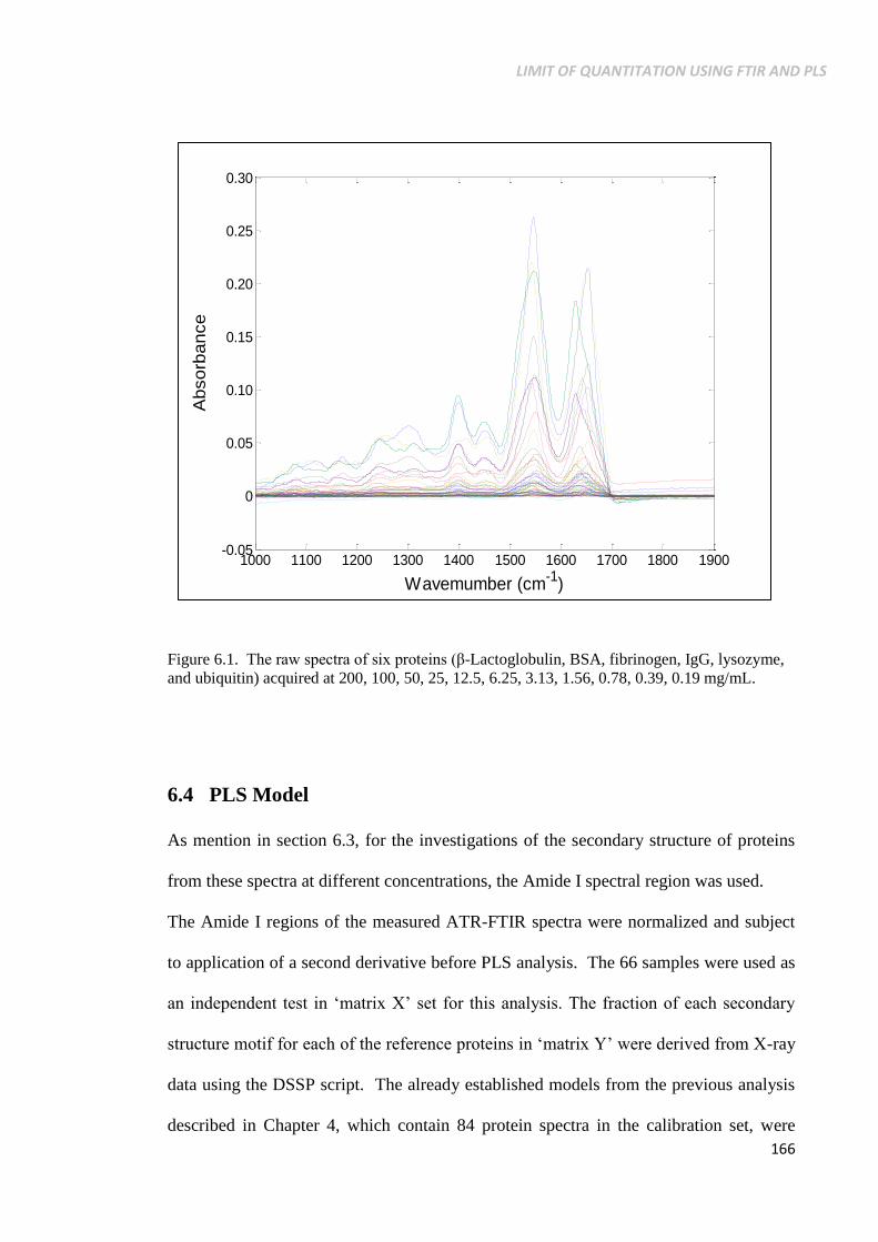
LIMIT OF QUANTITATION USING FTIR AND PLS
166
Figure 6.1. The raw spectra of six proteins (β-Lactoglobulin, BSA, fibrinogen, IgG, lysozyme,
and ubiquitin) acquired at 200, 100, 50, 25, 12.5, 6.25, 3.13, 1.56, 0.78, 0.39, 0.19 mg/mL.
6.4 PLS Model
As mention in section 6.3, for the investigations of the secondary structure of proteins
from these spectra at different concentrations, the Amide I spectral region was used.
The Amide I regions of the measured ATR-FTIR spectra were normalized and subject
to application of a second derivative before PLS analysis. The 66 samples were used as
an independent test in ‘matrix X’ set for this analysis. The fraction of each secondary
structure motif for each of the reference proteins in ‘matrix Y’ were derived from X-ray
data using the DSSP script. The already established models from the previous analysis
described in Chapter 4, which contain 84 protein spectra in the calibration set, were
1000 1100 1200 1300 1400 1500 1600 1700 1800 1900-0.05
0
0.05
0.10
0.15
0.20
0.25
0.30
Absorb
ance
Wavemumber (cm-1
)

USING REGRESSION ANALYSES FOR THE DETERMINATION
OF PROTEIN STRUCTURE FROM FTIR SPECTRA 167
used for structural determination for the different protein concentrations. This model
satisfies the condition described by eq. (1.3) in Chapter 1. The PLS models were
validated, as specified in Chapter 1, with 10-fold (segments) specified. Again, this
algorithm aims to maximize the association between the secondary structure of proteins
in matrix X and their DSSP values in matrix Y while minimizing E (error). The
principles underlying the PLS technique were described in Chapter 1.
6.5 Results and discussion
High quality FTIR spectra of proteins are usually obtained using high protein
concentrations. Dong, et al. (136) reported that higher than 12 mg/mL of protein
concentration is required to obtain good quality infrared spectra, and D’Antonio, et
al.(106) also reported that concentrations at 25mg/ml or higher provides good precision
and reproducibility. In Figure 6.1, it can be seen that the quality of the spectrum
decreases with decrease in concentration, as expected, and this, as Dong, et al. argued in
their study, has made FTIR spectroscopy not quite as useful in the study of protein at
low concentration. It also makes it difficult to compare spectra measured by FTIR and
circular dichroism. With the use of Multivariate Regression (MVR) analysis such as
PLS, the contributions of weaker bands can be equally as significant as those of stronger
bands by using normalization. Spectral data points were scaled to values between 0 and
1 for all spectra, making them compatible with each other and useful for multivariate
analysis.(88)
Proteins used for the analysis of secondary structure in the previous work performed in
this research and presented in the previous chapters were collected at a uniform
concentration of 50mg/mL; this was to ensure high quality spectra. However, the pre-

LIMIT OF QUANTITATION USING FTIR AND PLS
168
processing methods such as normalization (as seen in Figure 6.2 of the Amide I region)
and second derivative ensures that, even at low concentration, PLS can extract the latent
variables that explain the structural variations in the dataset.(239)
Figure 6.2. Spectra of 66 proteins in the Amide I region in concentrations between 200 mg/mL
and 0.19 mg/mL and scaled for PLS analysis.
Figure 6.3 shows the scaled spectra of Lysozyme acquired at the concentration of 200
mg/mL, 50 mg/mL, and 0.19 mg/mL. While all 3 spectra show peaks at about 1654 cm-
1, there are noticeable difference in the spectra; the spectrum at the lower concentration
(0.19 mg/mL) shows peaks at 1610 cm-1
and 1680 cm-1
and seems to have more
structural variations than the spectra of the 50 mg/mL and 200 mg/mL. The spectrum of
200 mg/mL appears broader than the other two spectra in the plot.
1600 1620 1640 1660 1680 17000
0.1
0.2
0.3
0.4
0.5
0.6
0.7
0.8
0.9
1
Norm
alized inte
nsity
Wavenumber (cm-1)
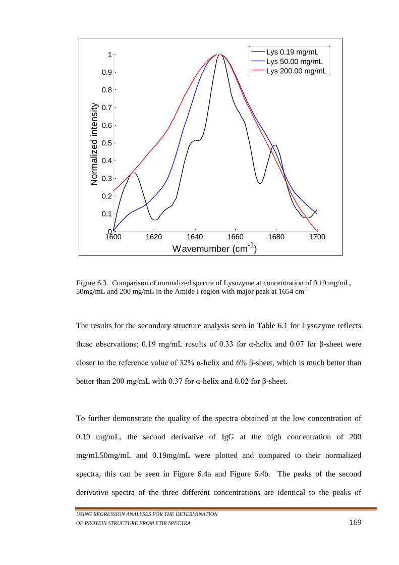
USING REGRESSION ANALYSES FOR THE DETERMINATION
OF PROTEIN STRUCTURE FROM FTIR SPECTRA 169
Figure 6.3. Comparison of normalized spectra of Lysozyme at concentration of 0.19 mg/mL,
50mg/mL and 200 mg/mL in the Amide I region with major peak at 1654 cm-1
The results for the secondary structure analysis seen in Table 6.1 for Lysozyme reflects
these observations; 0.19 mg/mL results of 0.33 for α-helix and 0.07 for β-sheet were
closer to the reference value of 32% α-helix and 6% β-sheet, which is much better than
better than 200 mg/mL with 0.37 for α-helix and 0.02 for β-sheet.
To further demonstrate the quality of the spectra obtained at the low concentration of
0.19 mg/mL, the second derivative of IgG at the high concentration of 200
mg/mL50mg/mL and 0.19mg/mL were plotted and compared to their normalized
spectra, this can be seen in Figure 6.4a and Figure 6.4b. The peaks of the second
derivative spectra of the three different concentrations are identical to the peaks of
1600 1620 1640 1660 1680 17000
0.1
0.2
0.3
0.4
0.5
0.6
0.7
0.8
0.9
1
Wavemumber (cm-1
)
No
rma
lize
d in
ten
sity
Lys 0.19 mg/mL
Lys 50.00 mg/mL
Lys 200.00 mg/mL
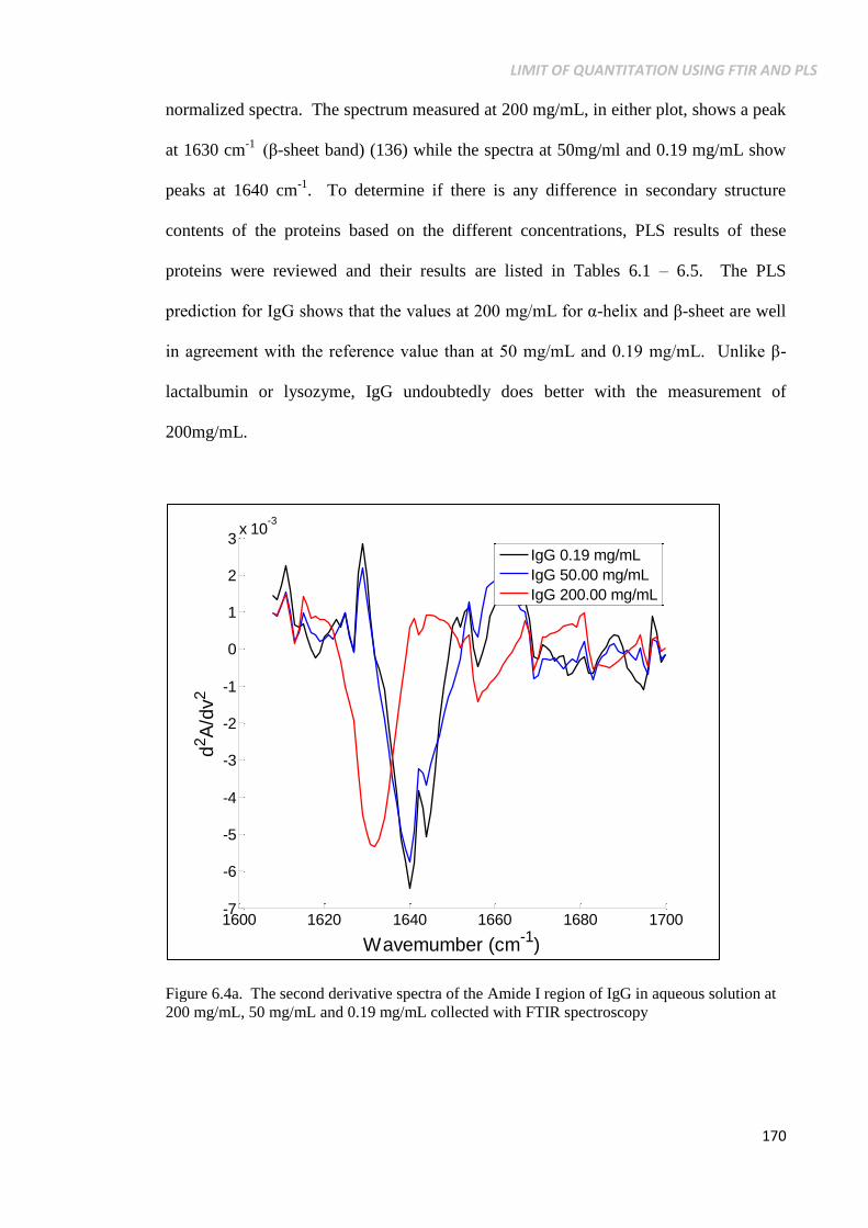
LIMIT OF QUANTITATION USING FTIR AND PLS
170
normalized spectra. The spectrum measured at 200 mg/mL, in either plot, shows a peak
at 1630 cm-1
(β-sheet band) (136) while the spectra at 50mg/ml and 0.19 mg/mL show
peaks at 1640 cm-1
. To determine if there is any difference in secondary structure
contents of the proteins based on the different concentrations, PLS results of these
proteins were reviewed and their results are listed in Tables 6.1 – 6.5. The PLS
prediction for IgG shows that the values at 200 mg/mL for α-helix and β-sheet are well
in agreement with the reference value than at 50 mg/mL and 0.19 mg/mL. Unlike β-
lactalbumin or lysozyme, IgG undoubtedly does better with the measurement of
200mg/mL.
Figure 6.4a. The second derivative spectra of the Amide I region of IgG in aqueous solution at
200 mg/mL, 50 mg/mL and 0.19 mg/mL collected with FTIR spectroscopy
1600 1620 1640 1660 1680 1700-7
-6
-5
-4
-3
-2
-1
0
1
2
3x 10
-3
Wavemumber (cm-1
)
d2A
/dv
2
IgG 0.19 mg/mL
IgG 50.00 mg/mL
IgG 200.00 mg/mL

USING REGRESSION ANALYSES FOR THE DETERMINATION
OF PROTEIN STRUCTURE FROM FTIR SPECTRA 171
Figure 6.4b. The normalized spectra of the Amide I region of IgG in aqueous solution at 200
mg/mL, 50 mg/mL and 0.19 mg/mL collected with FTIR spectroscopy.
The PLS result for the secondary structure contents of the six proteins used in this
analysis are listed in Tables 6.1 - 6.5. The bar graphs have been colour coded for ease
of review. The left hand black bar for each protein result is the reference value from
DSSP analysis of X-ray crystallographic data for that protein and the white bar in black
outline (50 mg/mL) is the concentration used for the prediction model.
IgG gave the most inconsistent results for the measured spectra. Gorga, et al.(207)
reported that the secondary structure analysis of proteins with low amounts of α-helix
such as IgG can be difficult to determine with CD spectra; however, secondary structure
composition of IgG FTIR spectra from this analysis compared to the corresponding
DSSP-derived reference set values was within ±0.05 accuracy (see Tables 6.1 – 6.5 for
1600 1620 1640 1660 1680 17000
0.1
0.2
0.3
0.4
0.5
0.6
0.7
0.8
0.9
1
Wavemumber (cm-1)
Norm
aliz
ed inte
nsity
IgG 0.19 mg/mL
IgG 50.00 mg/mL
IgG 200.00 mg/mL

LIMIT OF QUANTITATION USING FTIR AND PLS
172
secondary structure predictions). The predicted value of α-helix for IgG at 0.19 mg/mL
(α-helix: 0.03, β-sheet: 0.40) was low but the result at 0.39 mg/mL (α-helix: 0.07, β-
sheet: 0.39) obtained from this analysis were in agreement with Circular Dichroism
(CD) results for α-helix (8%) and β-sheet (41.3%) provided by Tetin et al.;(240)
although the concentration used for the CD measurement was not stated, CD spectra
are normally collected at 0.1 - 0.2 mg/mL. β-lactoglobulin results were in reasonable
agreement with X-ray crystallography values for all structural types for concentrations
between 0.19 and 1.56 mg/mL (See Tables 6.1 -6.4 for values). Ubiquitin, at higher
concentrations (0.50 mg/mL, 100 mg/mL, 200 mg/mL) had poorer α-helix results (0.20,
0.19, 0.24) respectively, as compared to the reference value of 0.16. Lysozyme, with a
major peak at 1654 cm-1
due to the presence of α-helix, gave results similar to the
structure of X-ray crystallography (within ±0.05 accuracy) for all concentrations.
Lysozyme results at 0.19 mg/mL (α-helix:0.33, β-sheet: 0.07) compared with X-ray
Crystallography values used for this study (α-helix = 0.32, β-sheet: 0.06) were also
comparable to (Chen, et al.) (241) results given for α-helix and β-sheet content from
CD (α=0.37, β= 0.11) with X-ray crystallography values of (α= 0.41, β=0.16).
Fibrinogen maintained its accurate results for higher concentrations (3.13 mg/mL to
200mg/mL) for the prediction of α-helix and β-sheet but also had very good results from
the lower concentration. These results can be viewed in Tables 6.1 – 6.5. BSA also had
very good result with lower protein concentrations from 0.19mg/mL up to 6.25 mg/mL.
It appears that the all α-proteins gave consistent results for the secondary structure
predictions across the board except for the prediction of β-sheet content. Overall,
results at lower concentrations for FTIR are consistent with that of their reference
protein values from X-ray crystallography and also with CD results for the compared

USING REGRESSION ANALYSES FOR THE DETERMINATION
OF PROTEIN STRUCTURE FROM FTIR SPECTRA 173
proteins given above.(241, 242) Overall, the results shown in Tables 6.1 – 6.5 are not
concentration dependent, and this quite evident with 310-helix (Table 6.3) where
sometimes proteins of lower and higher concentrations had more accurate results than
the concentrations in the middle; therefore the randomness seen in the data values may
be due to noise or systematic error due to interference during spectral measurement.

LIMIT OF QUANTITATION USING FTIR AND PLS
174
α-h
eli
x
Pro
tein
Na
me
PD
B V
alu
e0
.19
mg
/mL
0.3
9 m
g/m
L0
.78
mg
/mL
1.5
6 m
g/m
L3
.13
mg
/mL
6.2
5 m
g/m
L1
2.2
5 m
g/m
L2
5.0
0 m
g/m
L5
0.0
0 m
g/m
L1
00
.00
mg
/mL
20
0.0
0 m
g/m
L
β-L
acto
glo
bulin
0.1
00.1
00.1
00.1
00.1
10.1
10.1
20.0
70.1
10.1
20.1
00.0
8
BS
A0.7
00.6
90.7
10.7
20.7
10.7
20.6
90.7
40.6
40.6
70.7
10.7
0
Fib
rino
gen
(b
ovin
e p
lasm
a)0.7
00.7
50.7
30.7
00.6
60.6
60.6
40.6
70.6
40.7
10.7
00.7
1
IgG
(H
um
an)
0.0
80.0
30.0
70.1
10.0
80.1
20.0
30.0
40.1
20.0
60.1
00.0
8
Lyso
zym
e (C
hic
hen
egg)
0.3
20.3
30.3
10.3
10.3
00.3
40.3
10.3
60.3
60.2
80.3
20.3
7
Ub
iquitin
(b
ovin
e)0.1
60.1
70.1
50.2
00.1
60.1
40.1
10.1
60.1
40.2
00.1
90.2
4
0.0
0
0.1
0
0.2
0
0.3
0
0.4
0
0.5
0
0.6
0
0.7
0
0.8
0
β-L
act
ogl
ob
uli
nB
SAFi
bri
no
gen
(b
ovi
ne
pla
sma)
IgG
(H
um
an)
Lyso
zym
e (C
hic
he
n e
gg)
Ub
iqu
itin
(b
ovi
ne
)
PD
B V
alu
e
0.1
9 m
g/m
L
0.3
9 m
g/m
L
0.7
8 m
g/m
L
1.5
6 m
g/m
L
3.1
3 m
g/m
L
6.2
5 m
g/m
L
12
.25
mg/
mL
25
.00
mg/
mL
50
.00
mg/
mL
10
0.00
mg/
mL
20
0.00
mg/
mL
Tab
le 6
.1. P
LS
res
ult
s of
α-h
elix
co
nte
nt
of
6 p
rote
ins.
F
TIR
sp
ectr
a w
ere
use
d f
or
this
anal
ysi
s. E
ach p
rote
in
spec
tra
was
coll
ecte
d a
t co
nce
ntr
atio
ns
rangin
g f
rom
0.1
9 m
g/m
L t
o 2
00 m
g/m
L.

USING REGRESSION ANALYSES FOR THE DETERMINATION
OF PROTEIN STRUCTURE FROM FTIR SPECTRA 175
β-Sh
eet
Pro
tein
Nam
eP
DB
Val
ue0.
19 m
g/m
L0.
39 m
g/m
L0.
78 m
g/m
L1.
56 m
g/m
L3.
13 m
g/m
L6.
25 m
g/m
L12
.25
mg/
mL
25.0
0 m
g/m
L50
.00
mg/
mL
100.
00 m
g/m
L20
0.00
mg/
mL
β-La
ctog
lobu
lin0.
420.
400.
430.
440.
400.
420.
410.
390.
400.
400.
390.
38
BSA
0.00
0.00
0.01
-0.0
30.
01-0
.01
-0.0
7-0
.01
0.04
0.05
0.06
0.06
Fibr
inog
en (b
ovin
e pl
asm
a)0.
020.
070.
07-0
.07
0.07
0.02
0.05
0.03
0.03
0.02
0.03
0.02
IgG
(Hum
an)
0.37
0.40
0.39
0.40
0.33
0.35
0.37
0.39
0.40
0.41
0.39
0.38
Lyso
zym
e (C
hich
en e
gg)
0.06
0.07
0.08
0.08
0.05
0.05
0.03
0.06
0.07
0.06
0.02
0.02
Ubi
quiti
n (b
ovin
e)0.
310.
330.
330.
300.
320.
320.
260.
300.
280.
310.
280.
21
-0.1
0
0.00
0.10
0.20
0.30
0.40
0.50
β-L
acto
glob
ulin
BSA
Fibr
inog
en (
bovi
ne p
lasm
a)Ig
G (H
uman
)L
ysoz
yme
(Chi
chen
egg
)U
biqu
itin
(bov
ine)
PDB
Val
ue
0.19
mg/
mL
0.39
mg/
mL
0.78
mg/
mL
1.56
mg/
mL
3.13
mg/
mL
6.25
mg/
mL
12.2
5 m
g/m
L
25.0
0 m
g/m
L
50.0
0 m
g/m
L
100.
00 m
g/m
L
200.
00 m
g/m
L
Tab
le 6
.2. P
LS
res
ult
s of
β-s
hee
t co
nte
nt
of
6 p
rote
ins.
F
TIR
spec
tra
wer
e use
d f
or
this
an
alysi
s. E
ach
pro
tein
sp
ectr
a w
as c
oll
ecte
d a
t co
nce
ntr
atio
ns
rangin
g f
rom
0.1
9 m
g/m
L t
o 2
00
mg/m
L.

LIMIT OF QUANTITATION USING FTIR AND PLS
176
31
0-h
elix
Pro
tein
Na
me
PD
B V
alu
e0
.19
mg
/mL
0.3
9 m
g/m
L0
.78
mg
/mL
1.5
6 m
g/m
L3
.13
mg
/mL
6.2
5 m
g/m
L1
2.2
5 m
g/m
L2
5.0
0 m
g/m
L5
0.0
0 m
g/m
L1
00
.00
mg
/mL
20
0.0
0 m
g/m
L
β-L
acto
glo
bul
in0.
060.
060.
060.
060.
060.
060.
050.
050.
050.
050.
050.
04
BS
A0.
040.
040.
040.
050.
040.
030.
030.
040.
050.
050.
050.
05
Fib
rino
gen
(bo
vine
pla
sma)
0.02
0.03
0.02
0.01
0.03
0.03
0.02
0.02
0.01
0.01
0.04
0.03
IgG
(H
uman
)0.
040.
050.
050.
050.
030.
050.
050.
050.
050.
050.
050.
04
Lys
ozy
me
(Chi
chen
egg
)0.
100.
100.
100.
100.
090.
110.
100.
090.
100.
090.
090.
09
Ub
iqui
tin (
bo
vine
)0.
080.
070.
080.
080.
080.
090.
090.
070.
070.
080.
070.
06
0
0.050.
1
0.150.
2
0.250.
3
0.350.
4
0.450.
5
β-La
ctog
lobu
linBS
AFi
brin
ogen
IgG
(Hum
an)
Lyso
zym
e (C
hich
en e
gg)
Ubi
quiti
n
PDB
Valu
e
0.19
mg/
mL
0.39
mg/
mL
0.78
mg/
mL
1.56
mg/
mL
3.13
mg/
mL
6.25
mg/
mL
12.2
5mg/
mL
25.0
0mg/
mL
50.0
0mg/
mL
100.
00m
g/m
L
200.
00m
g/m
L
0.00
0.02
0.04
0.06
0.08
0.10
0.12
β-La
ctog
lobu
linBS
AFi
brin
ogen
(bov
ine
plas
ma)
IgG
(Hum
an)
Lyso
zym
e (C
hich
en e
gg)
Ubi
quiti
n (b
ovin
e)
PDB
Valu
e
0.19
mg/
mL
0.39
mg/
mL
0.78
mg/
mL
1.56
mg/
mL
3.13
mg/
mL
6.25
mg/
mL
12.2
5 m
g/m
L
25.0
0 m
g/m
L
50.0
0 m
g/m
L
100.
00 m
g/m
L
200.
00 m
g/m
L
Tab
le 6
.3. P
LS
res
ult
s of
31
0-h
elix
conte
nt
of
6 p
rote
ins.
F
TIR
spec
tra
wer
e u
sed f
or
this
anal
ysi
s.
Eac
h p
rote
in s
pec
tra
was
coll
ecte
d a
t co
nce
ntr
atio
ns
ran
gin
g f
rom
0.1
9 m
g/m
L t
o 2
00
mg/m
L.
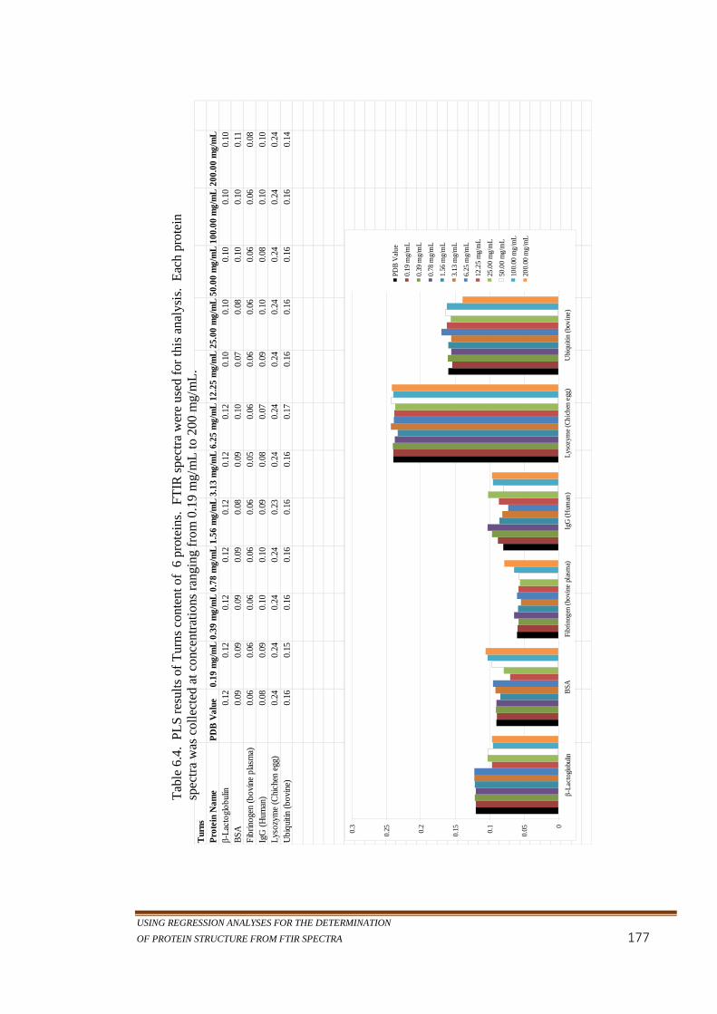
USING REGRESSION ANALYSES FOR THE DETERMINATION
OF PROTEIN STRUCTURE FROM FTIR SPECTRA 177
Tu
rns
Pro
tein
Na
me
PD
B V
alu
e0
.19
mg
/mL
0.3
9 m
g/m
L0
.78
mg
/mL
1.5
6 m
g/m
L3
.13
mg
/mL
6.2
5 m
g/m
L1
2.2
5 m
g/m
L2
5.0
0 m
g/m
L5
0.0
0 m
g/m
L1
00
.00
mg
/mL
20
0.0
0 m
g/m
L
β-L
acto
glo
bul
in0.
120.
120.
120.
120.
120.
120.
120.
100.
100.
100.
100.
10
BS
A0.
090.
090.
090.
090.
080.
090.
100.
070.
080.
100.
100.
11
Fib
rino
gen
(bo
vine
pla
sma)
0.06
0.06
0.06
0.06
0.06
0.05
0.06
0.06
0.06
0.06
0.06
0.08
IgG
(H
uman
)0.
080.
090.
100.
100.
090.
080.
070.
090.
100.
080.
100.
10
Lys
ozy
me
(Chi
chen
egg
)0.
240.
240.
240.
240.
230.
240.
240.
240.
240.
240.
240.
24
Ub
iqui
tin (
bo
vine
)0.
160.
150.
160.
160.
160.
160.
170.
160.
160.
160.
160.
14
0
0.050.1
0.150.2
0.250.3
β-L
acto
glob
ulin
BS
AF
ibri
nog
en (
bovi
ne p
lasm
a)Ig
G (
Hum
an)
Lys
ozym
e (C
hic
hen
egg
)U
biqu
itin
(bo
vin
e)
PD
B V
alu
e
0.19
mg/
mL
0.39
mg/
mL
0.78
mg/
mL
1.56
mg/
mL
3.13
mg/
mL
6.25
mg/
mL
12.2
5 m
g/m
L
25.0
0 m
g/m
L
50.0
0 m
g/m
L
100.
00 m
g/m
L
200.
00 m
g/m
L
Tab
le 6
.4. P
LS
res
ult
s of
Turn
s co
nte
nt
of
6 p
rote
ins.
F
TIR
spec
tra
wer
e use
d f
or
this
an
alysi
s.
Eac
h p
rote
in
spec
tra
was
coll
ecte
d a
t co
nce
ntr
atio
ns
rangin
g f
rom
0.1
9 m
g/m
L t
o 2
00 m
g/m
L.

LIMIT OF QUANTITATION USING FTIR AND PLS
178
Table 6.6 lists the R2 and overall root-mean-square error for prediction (δ); estimated (δ)
are less than 0.04 for 66 protein samples (11 different concentrations per protein). This
Oth
er
Pro
tein
Na
me
PD
B V
alu
e0
.19
mg
/mL
0.3
9 m
g/m
L0
.78
mg
/mL
1.5
6 m
g/m
L3
.13
mg
/mL
6.2
5 m
g/m
L1
2.2
5 m
g/m
L2
5.0
0 m
g/m
L5
0.0
0 m
g/m
L1
00
.00
mg
/mL
20
0.0
0 m
g/m
L
β-L
acto
glo
bul
in0.
290.
290.
290.
290.
310.
290.
300.
350.
360.
360.
350.
35
BS
A0.
160.
160.
150.
160.
150.
170.
150.
150.
170.
160.
170.
16
Fib
rino
gen
(bo
vine
pla
sma)
0.21
0.22
0.21
0.20
0.21
0.20
0.21
0.23
0.21
0.21
0.22
0.21
IgG
(H
uman
)0.
420.
430.
350.
360.
420.
400.
400.
420.
360.
430.
350.
35
Lys
ozy
me
(Chi
chen
egg
)0.
280.
270.
280.
280.
280.
280.
290.
280.
290.
280.
270.
27
Ub
iqui
tin (
bo
vine
)0.
280.
290.
290.
280.
280.
290.
250.
280.
280.
290.
270.
26
0
0.050.
1
0.150.
2
0.250.
3
0.350.
4
0.450.
5
β-La
ctog
lobu
linBS
AFi
brin
ogen
(bov
ine
plas
ma)
IgG
(Hum
an)
Lyso
zym
e (C
hich
en e
gg)
Ubi
quiti
n (b
ovin
e)
PDB
Valu
e
0.19
mg/
mL
0.39
mg/
mL
0.78
mg/
mL
1.56
mg/
mL
3.13
mg/
mL
6.25
mg/
mL
12.2
5 m
g/m
L
25.0
0 m
g/m
L
50.0
0 m
g/m
L
100.
00 m
g/m
L
200.
00 m
g/m
L
Tab
le 6
.5. P
LS
res
ult
s of
Dis
ord
ered
conte
nt
of
6 p
rote
ins.
F
TIR
spec
tra
wer
e use
d f
or
this
anal
ysi
s.
Eac
h p
rote
in s
pec
tra
was
coll
ecte
d a
t co
nce
ntr
atio
ns
ran
gin
g f
rom
0.1
9 m
g/m
L t
o 2
00
mg/m
L.
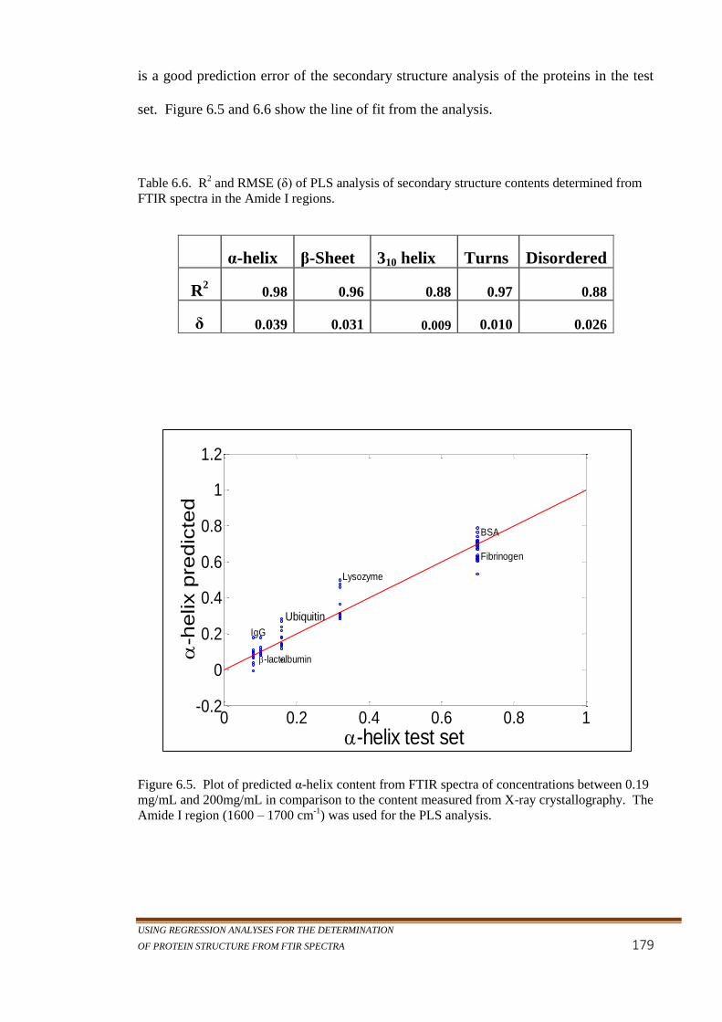
USING REGRESSION ANALYSES FOR THE DETERMINATION
OF PROTEIN STRUCTURE FROM FTIR SPECTRA 179
is a good prediction error of the secondary structure analysis of the proteins in the test
set. Figure 6.5 and 6.6 show the line of fit from the analysis.
Table 6.6. R2 and RMSE (δ) of PLS analysis of secondary structure contents determined from
FTIR spectra in the Amide I regions.
α-helix β-Sheet 310 helix Turns Disordered
R2 0.98 0.96 0.88 0.97 0.88
δ 0.039 0.031 0.009 0.010 0.026
Figure 6.5. Plot of predicted α-helix content from FTIR spectra of concentrations between 0.19
mg/mL and 200mg/mL in comparison to the content measured from X-ray crystallography. The
Amide I region (1600 – 1700 cm-1
) was used for the PLS analysis.
0 0.2 0.4 0.6 0.8 1-0.2
0
0.2
0.4
0.6
0.8
1
1.2
-helix test set
-h
elix p
redic
ted
BSA
Fibrinogen
Lysozyme
Ubiquitin
IgG
-lactalbumin
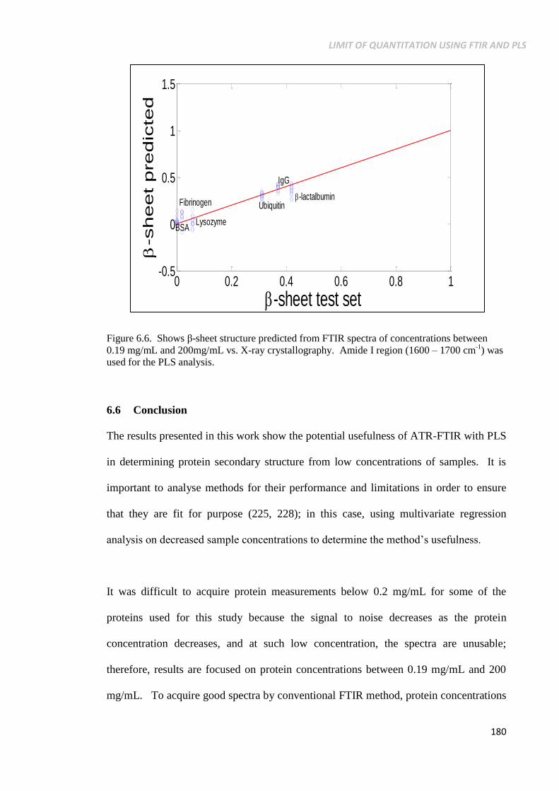
LIMIT OF QUANTITATION USING FTIR AND PLS
180
Figure 6.6. Shows β-sheet structure predicted from FTIR spectra of concentrations between
0.19 mg/mL and 200mg/mL vs. X-ray crystallography. Amide I region (1600 – 1700 cm-1
) was
used for the PLS analysis.
6.6 Conclusion
The results presented in this work show the potential usefulness of ATR-FTIR with PLS
in determining protein secondary structure from low concentrations of samples. It is
important to analyse methods for their performance and limitations in order to ensure
that they are fit for purpose (225, 228); in this case, using multivariate regression
analysis on decreased sample concentrations to determine the method’s usefulness.
It was difficult to acquire protein measurements below 0.2 mg/mL for some of the
proteins used for this study because the signal to noise decreases as the protein
concentration decreases, and at such low concentration, the spectra are unusable;
therefore, results are focused on protein concentrations between 0.19 mg/mL and 200
mg/mL. To acquire good spectra by conventional FTIR method, protein concentrations
0 0.2 0.4 0.6 0.8 1-0.5
0
0.5
1
1.5
-sheet test set
-sheet predic
ted
-lactalbumin
IgG
Ubiquitin
Lysozyme
Fibrinogen
BSA

USING REGRESSION ANALYSES FOR THE DETERMINATION
OF PROTEIN STRUCTURE FROM FTIR SPECTRA 181
above 10 mg/mL are normally used for proteins in H2O solutions due to the strong
absorption of water molecule in the Amide I region;(13, 136) However, technical
advances in FTIR spectroscopy have made it possible to routinely acquire protein
spectra from aqueous solutions at concentrations reportedly as low as 0.5mg/mL with
good signal to noise ratio,(136) therefore making it possible to compare FTIR results to
CD which is a well-established technique for determining the secondary structure of
proteins in solution. In addition, CD spectroscopy is limited by the strong overlap of β-
sheet, β-turns and unordered structure.(207)
Results from this study gave a RMSE of less than 0.04 for α-helix and β-sheet
prediction for samples collected at concentrations between 0.19 mg/mL and 200
mg/mL. These results are more accurate than the CD prediction results with RMSE of
0.06 – 0.1 for both α-helix and β-sheet (sample concentrations collected at 0.1 – 2.0
mg/mL).(136, 175, 177, 243, 244)
Again, this study was not done to determine the limit of detection of protein spectra by
ATR-FTIR, rather, it was done to determine how well multivariate regression analysis
methods like PLS can determine secondary structures from spectra of low
concentrations. The results derived from this study show that the combination of
second derivative and PLS analysis of FTIR spectra of proteins, has made it possible to
resolve peak intensities and statistically derive their secondary structure conformations
at even low concentrations.
CONCLUSION
182
7 Conclusion
This thesis has demonstrated that spectroscopic techniques can be used in conjunction
with multivariate analytical tools in order to achieve great results for the structural
analysis of proteins in solutions. Even though X-ray crystallography and NMR are used
to solve the three dimensional structures of proteins, they have their limitations; protein
crystallography is time consuming and many proteins do not readily crystalize, and protein
size limitation is an issue for NMR, besides, NMR is time consuming.(33, 210, 245,
246) Fourier transform infrared (FT-IR) spectroscopy is a rapid spectroscopic
technique that can give fingerprints of protein structures in solution, solid or gas phase.
It can be used to reduce the sample analysis period significantly due to its rapid spectral
measurement.(36, 121) However, FTIR spectra suffer from interfering background
signals that must be reduced or removed before any data analysis.(247, 248) There are
many methods used to remove background effects from the spectra, these include some
of the methods used in this thesis: baseline correction, Multiplicative Scattered
Correction (MSC), Standard Normal Variate (SNV), and Second Derivative. There is
also a need to analyse the underlying biological differences between the identified FTIR
spectral regions and also to determine their secondary structures.(69, 249) Methods that
have been used to determine protein structure include band deconvolution and neural
networks (ANN) but their models are difficult to interpret.(250) MVA has proved to be
an appropriate tool to carry out the quantification of protein secondary structure from
their infrared spectra because of its simplicity and ability to reduce the data to a lower
dimension and extract the relevant information.(251, 252)
USING REGRESSION ANALYSES FOR THE DETERMINATION
OF PROTEIN STRUCTURE FROM FTIR SPECTRA 183
Myra Kinalwa(177) used similar methods on Raman spectra and achieved very good
results especially with the Amide I, II and III regions combined; however, the size of
the protein dataset was too small to validate the model with an independent test set.
Raman spectroscopy, a technique based on inelastic scattering of monochromatic light,
is making its mark as another vibrational spectroscopic method that has been
successfully used in the determination of the secondary structure of protein.(137, 253)
FTIR and Raman techniques provide complementary information; while Raman
spectroscopy may not have the H2O absorption in the Amide I region found in FTIR, its
signal to noise is inferior to FTIR absorption spectra and the quantitative results from
FTIR method are better.(254, 255)
In the first result chapter 3, FTIR spectra were obtained for proteins dissolved in H2O.
The absorbance spectra of predominantly α-helical, β-sheet and mixture of α and β
proteins were measured and analysed. This analysis made use of the strength of
Principal Component Analysis (PCA), an MVA classification method, on ATR-FTIR
spectra for classification of proteins into their natural groupings of All α, All β, α/β,
α+β, as defined by SCOP. SCOP (release 1.75) currently has 110800 Domains protein
domains classified into 1195 folds; this means there are 92.72 domains per fold.
Performing data classification on the SCOP folds will need lots of data; (256, 257)
therefore the analysis was limited to the protein class structure.
The variations in the samples used for this analysis were described by 4 PCs giving a
95.39% of the total variations in the data. The protein spectra classifications showed
strong groupings of proteins of α and β classes and those of mixed types not in any of
the two groups. The obtained PCA results using FTIR spectra were comparable or

CONCLUSION
184
even better than CD methods currently used for protein classification. ATR-FTIR
absorption spectra contain a great deal of information that can be utilized for
classification and identity determination of proteins and other biologic systems; for
example, qualitative analysis tools like PCA can be used in the identification of
biomarkers of several diseases like cancer, Alzheimer’s and other autoimmune disorders
due to changes in the secondary structure of their biomolecules.(258, 259)
In the second result Chapter 4, ATR-FTIR spectroscopy in combination with partial
least squares (PLS), a multivariate regression methods, was used to calibrate and
quantify different proteins in H2O; the calibration dataset covered Amide I, II and III
(1700cm – 1200 cm-1) regions of the protein spectra. The ATR-FTIR spectra showed
very good predictive value for the calibration (to within 0.01 to 0.05 RMSE) and the
independent test set prediction (from 0.01 – 0.12 RMSEP). Spectral features linked to
α-helix and β-sheet had excellent structural determination; structural features like 310
helix, turns and random coils were also elucidated with good results as listed in Chapter
4 and Appendix B of this thesis.
A version of PLS called interval PLS (iPLS) uses subintervals of the full spectrum.
Local models are built with intervals of the spectral region; the performance of the local
models is compared to that of the full spectrum model. By using intervals of the
spectrum, regions specific to each secondary structure motif can be identified. This use
of only the significant spectral regions can reducing spectral measurement time;
however, selection of the number of intervals that can yield an optimum result for each
motif can be time consuming. The iPLS result in this analysis, although useful, was not
as good as that of the traditional PLS model.
USING REGRESSION ANALYSES FOR THE DETERMINATION
OF PROTEIN STRUCTURE FROM FTIR SPECTRA 185
Many researchers focused their analysis on α-helix and β-sheet contents because these
spectral features are better abundant than 310-helix other structural types.(150) With
the use of second derivative, underlying spectral peaks can be resolved to identify their
positions whereby aiding in the multivariate regression analysis of different structural
motifs. One of the uses of statistical quantitative analysis in the biomedical field is in
pharmaceuticals to confirm their structural conformation from manufacturing to
distributions, including their shelf lives.(64, 69) Multivariate regression analysis can be
also combined with X-ray crystallography or NMR spectroscopy to derive information
from their protein measurements due to the reliability and accuracy of the statistical
method.(260) Three key advantages of MVA is the small sample size needed to train
the model, the method’s ability to handle multivariate data, and missing data in the
spectra;(261) however, PLS has a known fault of being sensitive to the number of
components used in the model; increasing the number of components or descriptors in
the model improves it’s fit but decreases its ability to fit new data well.(262) (Zeng and
Li)(263) pointed out that PLS cannot handle continuous streams data as all of the data
are loaded into memory. This incremental PLS for continuous streams of should help in
the analysis of large data sets and real-time data.
Chapter 5 illustrated the strength of using FTIR to distinguish between native and
unfolding proteins between pH 2.0 and pH 7.0 in increments of 0.5 pH levels. The PLS
calibration model established in Chapter 4 was used to elucidate the secondary structure
of the denatured α-Lactalbumin (α-LA) proteins at each pH. The second derivative
spectra showed important spectral changes that occurred during denaturation. Result
from the analysis in this study showed the structure of α-LA at the native state, the
absence of Ca2+
binding molecule (the apo-protein) where an intermediate form and the
structure of β-sheet diminished, and finally the formation of intramolecular anti-parallel
CONCLUSION
186
β-sheet in the acidic (A-state) protein. Proteins need to be in their native state to operate
efficiently, therefore; studying the changes in their aggregation stages may help in
understanding how proteins misfold.(183, 203) A related study done with Raman
spectroscopy using 2Dimensional Correlation (2DCOS) to study the spectral intensity
variations of α-lactalbumin within the pH ranges of 2 and 7 was successfully carried out
by Ashton and Blanch(254). The 2DCOS method was used to identify secondary
structure variations occurring in the different FTIR spectral bands of denatured α-LA.
In Chapter 6, the calibration model was applied to proteins of various concentrations to
determine their secondary structure. The main aim of this Chapter is to test the model
for its limit of quantification. It is clear that some proteins absorb well at low
concentrations; in general, multivariate regression analysis does a good job with
proteins at concentrations as low as 0.20 mg/mL. This method serves as a good
detection tool for forensic and other biomedical needs of detecting substances at low
concentrations.
One other popular types of multivariate analysis method used in the elucidation of
protein is Artificial Neural Network (ANN).(252) ANN is also popular for determining
the secondary structure of proteins from spectra; however, the methodology is not as
fast as PLS and not as easy to learn, moreover, overfitting can be stronger in neural
networks than in PLS because of the layers or neurons used for the analysis.(253)
In summary, FTIR has advantages over other widely used structural spectroscopic
methods like CD and NMR; FTIR is fast and easy to use and require very little sample.
The four result chapters in this thesis show how multivariate statistical analytical tools
like PLS and PCA can be used to obtain structural contents from ATR-FTIR spectra.

USING REGRESSION ANALYSES FOR THE DETERMINATION
OF PROTEIN STRUCTURE FROM FTIR SPECTRA 187
These results show that FT-IR spectroscopy can extend its applications in the
biotechnology industry as a rapid method for detection and quantification of substances,
especially for proteins in solution.

APPENDIX
188
8 References
1. Whitford D. Proteins: Structure and function. Hoboken, N.J.: John Wiley &
Sons; 2013.
2. Lehninger AL, Nelson DL, Cox MM. Lehninger principles of biochemistry.
New York, N.Y.: W. H. Freeman; 2008.
3. McMurry J. Fundamentals of organic chemistry: Cengage Learning; 2010.
4. Purves WK. Life, the science of biology: Sinauer Associates; 2004.
5. Clayden J, Greeves N, Warren S, P. W. Organic chemistry, Oxford, England:
Oxford University; 2000.
6. Degrève L, Fuzo CA, Caliri A. Extended secondary structures in proteins.
Biochimica et Biophysica Acta (BBA) - Proteins and Proteomics.
2014;1844(2):384-388.
7. Eidhammer I, Jonassen I, Taylor WR. Protein bioinformatics: An algorithmic
approach to sequence and structure analysis: J. Wiley & Sons; 2004.
8. Petsko GA, Ringe D. Protein structure and function: New Science Press;
2004.
9. Brändén CI, Tooze J. Introduction to protein structure: Garland Pub.; 1999.
10. Alberts B, Johnson A, Lewis J, Raff M, Robert K, et al. Molecular biology of
the cell. 4th. ed. New York: Garland Science; 2002.
11. Vieira-Pires RS, Morais-Cabral JH. 310-helices in channels and other
membrane proteins. The Journal of General Physiology. 2010;136(6):585-
592.
12. Barlow DJ, Thornton JM. Helix geometry in proteins. Journal of Molecular
Biology. 1988;201(3):601-619.
13. Kong J, Yu S. Fourier transform infrared spectroscopic analysis of protein
secondary structures. Acta Biochimica et Biophysica Sinica. 2007;39(8):549-
559.
14. Pain RH. Mechanisms of protein folding: Oxford University Press; 2000.
15. Heller BA, Gindt YM. A biochemical study of noncovalent forces in proteins
using phycocyanin from spirulina. Journal of Chemical Education.
2000;77(11):1458.
16. Fold classification based on structure-structure alignment of proteins.

USING REGRESSION ANALYSES FOR THE DETERMINATION
OF PROTEIN STRUCTURE FROM FTIR SPECTRA 189
17. Orengo CA, Michie AD, Jones S, Jones DT, Swindells MB, Thornton JM.
Cath – a hierarchic classification of protein domain structures. Structure.
1997;5(8):1093-1109.
18. Murzin AG, Brenner SE, Hubbard T, Chothia C. Scop: A structural
classification of proteins database for the investigation of sequences and
structures. Journal of Molecular Biology. 1995;247(4):536-540.
19. Yu X, Wang C, Li Y. Classification of protein quaternary structure by
functional domain composition. BMC Bioinformatics. 2006;7(1):187.
20. Squire J, Parry DAD. Fibrous proteins: Muscle and molecular motors:
Elsevier; 2005.
21. Ruso JM, Attwood D, García M, Prieto G, Sarmiento F, Taboada P, et al.
Interaction of amphiphilic propranolol hydrochloride with haemoglobin and
albumin in aqueous solution. Langmuir : The ACS Journal of Surfaces and
Colloids. 2000;16(26):10449-10455.
22. Richter JD. Mrna formation and function: Elsevier Science; 1997.
23. Permiakov EA, Permi akov EA. Alpha-lactalbumin: Nova Science Publishers;
2005.
24. Paci E, Smith LJ, Dobson CM, Karplus M. Exploration of partially unfolded
states of human α-lactalbumin by molecular dynamics simulation. Journal of
Molecular Biology. 2001;306(2):329-347.
25. Spiro RG. Protein glycosylation: nature, distribution, enzymatic formation,
and disease implications of glycopeptide bonds. Glycobiology.
2002;12(4):43R-56R.
26. Ovádi J, Orosz F. Protein folding and misfolding: Neurodegenerative
diseases: Neurodegenerative diseases: Springer; 2008.
27. Shenolikar S. Protein phosphorylation in health and disease: Elsevier
Science & Technology Books; 2012.
28. Martin I, Kim JW, Lee BD, Kang HC, Xu JC, Jia H, et al. Ribosomal protein
s15 phosphorylation mediates lrrk2 neurodegeneration in parkinson's disease.
Cell. 2014;157(2):472-485.
29. Cohen P. The role of protein phosphorylation in human health and disease. .
European Journal of Biochemistry. 2001;268(19):5001-5010.
30. Muller P, Ruckova E, Halada P, Coates PJ, Hrstka R, Lane DP, et al. C-
terminal phosphorylation of hsp70 and hsp90 regulates alternate binding to
co-chaperones chip and hop to determine cellular protein folding/degradation
balances. Oncogene. 2013;32(25):3101-3110.
31. Dobson CM. Protein folding and misfolding. Nature. 2003;426(6968):884-
890.

APPENDIX
190
32. Seddon AM, Curnow P, Booth PJ. Membrane proteins, lipids and detergents:
Not just a soap opera. Biochimica et Biophysica Acta (BBA) - Biomembranes.
2004;1666(1–2):105-117.
33. Barton GJ. Protein secondary structure prediction. Current Opinion in
Structural Biology. 1995;5(3):372-376.
34. Jackson M, Mantsch H. The use and misuse of FTIR spectroscopy in the
determination of protein structure. Critical Reviews in Biochemistry and
Molecular Biology. 1995;30(2):95-120.
35. Smith BC. Fundamentals of Fourier transform infrared spectroscopy, second
edition: Taylor & Francis; 2011.
36. Haris PI, Severcan F. FTIR spectroscopic characterization of protein structure
in aqueous and non-aqueous media. Journal of Molecular Catalysis B:
Enzymatic. 1999;7(1–4):207-221.
37. Magazu S, Calabro E. Studying the electromagnetic-induced changes of the
secondary structure of bovine serum albumin and the bioprotective
effectiveness of trehalose by Fourier transform infrared spectroscopy. The
Journal of Physical Chemistry B. 2011;115(21):6818-6826.
38. Smith E, Dent G. Modern Raman spectroscopy: A practical approach:
Wiley; 2013.
39. Cai S, Singh BR. Identification of β-turn and random coil amide iii infrared
bands for secondary structure estimation of proteins. Biophysical Chemistry.
1999;80(1):7-20.
40. Dunuwila DD, Berglund KA. Identification of infrared spectral features
related to solution structure for utilization in solubility and supersaturation
measurements. Organic Process Research & Development. 1997;1(5):350-
354.
41. Dousseau F, Pezolet M. Determination of the secondary structure content of
proteins in aqueous solutions from their amide i and amide ii infrared bands.
Comparison between classical and partial least-squares methods.
Biochemistry. 1990;29(37):8771-8779.
42. Stuart BH. A FFourier transform infrared spectroscopic study of the
secondary structure of myelin basic protein in reconstituted myelin.
Biochemistry and molecular biology international. 1996;38(4):839-845.
43. Davis R, Mauer IJ. Fourier transform infrared (FTIR) spectroscopy: A rapid
tool for detection and analysis of foodborne pathogenic bacteria. In: A. M-V,
editor. Current research, technology and education topics in applied
microbiology and microbial biotechnology. 2: ormatex Research Center;
2010.582-1594.
44. Nishikida K, Nishio E, Hannah RW. Selected applications of modern ft-ir
techniques: Taylor & Francis; 1996.

USING REGRESSION ANALYSES FOR THE DETERMINATION
OF PROTEIN STRUCTURE FROM FTIR SPECTRA 191
45. Pretsch E, Bühlmann P, Badertscher M. Structure determination of organic
compounds: Tables of spectral data: Springer; 2009.
46. Ramer G, Lendl B. Attenuated total reflection Fourier transform infrared
spectroscopy. Encyclopedia of Analytical Chemistry: John Wiley & Sons,
Ltd; 2006.
47. Schrader B. Infrared and Raman Spectroscopy: Methods and Applications:
Wiley; 2008.
48. Glassford SE, Byrne B, Kazarian SG. Recent applications of ATR-FTIR
spectroscopy and imaging to proteins. Biochimica et Biophysica Acta (BBA) -
Proteins and Proteomics. 2013;1834(12):2849-2858.
49. Goldberg ME, Chaffotte AF. Undistorted structural analysis of soluble
proteins by attenuated total reflectance infrared spectroscopy. Protein
Science. 2005;14(11):2781-2792.
50. Arrondo JLR, Goñi FM. Structure and dynamics of membrane proteins as
studied by infrared spectroscopy. Progress in Biophysics and Molecular
Biology. 1999;72(4):367-405.
51. Raman S, Lange OF, Rossi P, Tyka M, Wang X, Aramini J, et al. NMR
structure determination for larger proteins using backbone-only data. Science.
2010;327(5968):1014-1018.
52. Wu TD, Schmidler SC, Hastie T, Brutlag DL. Journal of Computational
Biology. 1998;5(3):585-595.
53. Efimova YM, Haemers S, Wierczinski B, Norde W, Well AAv. Stability of
globular proteins in h2o and d2o. Biopolymers. 2007;85(3):264-273.
54. Keiderling TA, Wang B, Urbanova M, Pancoska P, Dukor RK. Empirical
studies of protein secondary structure by vibrational circular dichroism and
related techniques. Alpha-lactalbumin and lysozyme as examples. Faraday
Discussions. 1994(99):263-285
55. Downer NW, Bruchman TJ, Hazzard JH. Infrared spectroscopic study of
photoreceptor membrane and purple membrane. Protein secondary structure
and hydrogen deuterium exchange. J Biol Chem. 1986;261(8):3640-3647.
56. Joosten R, te Beek T, Krieger E, Hekkelman M, Hooft R, Schneider R, et al.
A series of pdb related databases for everyday needs 2011 [cited 2013 12
Dec]. Available from: http://dx.doi.org/10.1093/nar/gkq1105.
57. Strasfeld DB, Ling YL, Shim S-H, Zanni MT. Tracking fiber formation in
human islet amyloid polypeptide with automated 2d-ir spectroscopy. Journal
of the American Chemical Society. 2008;130(21):6698-6699.
58. Pirovano W, Heringa J. Protein secondary structure prediction. Methods in
Molecular Biology. 2010;609:327-348.
APPENDIX
192
59. Wang F, Liu AP, Ren FZ, Zhang XY, Stephanie C, Zhang LD, et al. FTIR
analysis of protein secondary structure in cheddar cheese during ripening.
Guang pu. 2011;31(7):1786-1789.
60. Higuchi II, Eguchi S. The influence function of principal component analysis
by self-organizing rule. Neural Computation. 1998;10(6):1435-1444.
61. Candolfi A, De Maesschalck R, Jouan-Rimbaud D, Hailey PA, Massart DL.
The influence of data pre-processing in the pattern recognition of excipients
near-infrared spectra. Elsevier. 1999. 115-132.
62. Ge Y-S, Jin C, Song Z, Zhang J-Q, Jiang F-L, Liu Y. Multi-spectroscopic
analysis and molecular modeling on the interaction of curcumin and its
derivatives with human serum albumin: A comparative study. Spectrochimica
Acta Part A: Molecular and Biomolecular Spectroscopy. 2014;124(0):265-
276.
63. Wold S. Chemometrics, why, what and where to next? Journal of
Pharmaceutical and Biomedical Analysis. 1991;9(8):589-596.
64. Brereton RG. Applied chemometrics for scientists: Wiley; 2007.
65. Jorgensen A. Clustering excipient near infrared spectra using different
chemometric methods Dept. of Pharmacy, University of Helsinki2000 [cited
2014 12 Jan.]. Available from:
http://www.pharmtech.helsinki.fi/seminaarit/vanhat/annajorgensen.pdf.
66. Yao F, Coquery J, Le Cao KA. Independent principal component analysis for
biologically meaningful dimension reduction of large biological data sets.
BMC Bioinformatics. 2012;13:24.
67. Uceda Otero EP, Eliel GSN, Fonseca EJS, Hickmann JM, Rodarte R, Barreto
E, et al. Study of cancer cell lines with Fourier transform infrared
(FTIR)/vibrational absorption (va) spectroscopy. Current Physical Chemistry.
2013;3(1).
68. Rusak DA, Brown LM, Martin SD. Classification of vegetable oils by
principal component analysis of FTIR spectra. Journal of Chemical
Education. 2003;80(5):541.
69. Ami D, Doglia SM, Mereghetti P. Multivariate analysis for Fourier
transform infrared spectra of complex biological systems and processes.
InTech. 2013.
70. Hemmateenejad B, Akhond M, Samari F. A comparative study between pcr
and pls in simultaneous spectrophotometric determination of diphenylamine,
aniline, and phenol: Effect of wavelength selection. Spectrochimica Acta Part
A: Molecular and Biomolecular Spectroscopy. 2007;67(3–4):958-965.
71. Phatak A. A user-friendly guide to multivariate calibration and
classificationtion, t. Næs, t. Isaksson, t. Fearn, t. Davies: Chichester: Nir
USING REGRESSION ANALYSES FOR THE DETERMINATION
OF PROTEIN STRUCTURE FROM FTIR SPECTRA 193
publications. Chemometrics and Intelligent Laboratory Systems.
2004;71(1):79-81.
72. Hori R, Sugiyama J. A combined FTIR microscopy and principal component
analysis on softwood cell walls. Carbohydrate Polymers. 2003;52(4):449-
453.
73. David CC, Jacobs DJ. Principal component analysis: A method for
determining the essential dynamics of proteins. Methods in Molecular
Biology. 2014;1084:193-226.
74. Shojaei M, Mirmohseni A, Farbodi M. Application of a quartz crystal
nanobalance and principal component analysis for the detection and
determination of histidine. Analytical and Bioanalytical Chemistry.
2008;391(8):2875-2880.
75. Wold S, Esbensen K, Geladi P. Principal component analysis. Chemometrics
and Intelligent Laboratory Systems. 1987;2(1–3):37-52.
76. Burstyn I. Principal component analysis is a powerful instrument in
occupational hygiene inquiries. The Annals of Occupational Hygiene.
2004;48(8):655-661.
77. Carey RN, Wold S, Westgard JO. Principal component analysis: An
alternative to "referee" methods in method comparison studies. Analytical
Chemistry. 1975;47(11):1824-1829.
78. Campins-Falco P, Blasco-Gomez F, Bosch-Reig F, Gallo-Martinez L.
Principal component analysis for the selection of variables in the application
of the h-point and generalised h-point standard addition method. Talanta.
2000;53(2):317-330.
79. Varnek A, Baskin I. Machine learning methods for property prediction in
chemoinformatics: Quo vadis? Journal of Chemical Information and
Modeling. 2012;52(6):1413-1437.
80. Bai L, Gao B, Tian S, Cheng Y, Chen Y, Tian GY, et al. A comparative study
of principal component analysis and independent component analysis in eddy
current pulsed thermography data processing. The Review of Scientific
instruments. 2013;84(10):104901.
81. Craig A, Merlic CA. Introduction to ir spectra: UCLA chemistry and
Biochemistry 1997 [cited 2010 20th Nov]. Available from: Available from:
http://www.chem.ucla.edu/~webspectra/irintro.html.
82. Delwiche SR, Reeves JB, 3rd. A graphical method to evaluate spectral
preprocessing in multivariate regression calibrations: Example with savitzky-
golay filters and partial least squares regression. Applied Spectroscopy.
2010;64(1):73-82.

APPENDIX
194
83. Berg R, Hoefsloot H, Westerhuis J, Smilde A, Werf M. Centering, scaling,
and transformations: Improving the biological information content of
metabolomics data. BMC Genomics. 2006;7(1):1-15.
84. Noda I. Scaling techniques to enhance two-dimensional correlation spectra.
Journal of Molecular Structure. 2008;883–884(0):216-227.
85. Karpievitch Y, Dabney A, Smith R. Normalization and missing value
imputation for label-free lc-ms analysis. BMC Bioinformatics. 2012;13(Suppl
16):S5.
86. Lacher DA. Interpretation of laboratory results using multidimensional
scaling and principal component analysis. Annals of Clinical and Laboratory
Science. 1987;17(6):412-417.
87. McPhie P. Concentration-independent estimation of protein secondary
structure by circular dichroism: A comparison of methods. Anal Biochem.
2008;375(2):379-381.
88. Craig A, Cloarec O, Holmes E, Nicholson JK, Lindon JC. Scaling and
normalization effects in NMR spectroscopic metabonomic data sets.
Analytical Chemistry. 2006;78(7):2262-2267.
89. Martens H, Naes T. Multivariate calibration: Wiley; 1989.
90. Perez-Guaita D, Kuligowski J, Quintas G, Garrigues S, Guardia Mde L.
Modified locally weighted--partial least squares regression improving clinical
predictions from infrared spectra of human serum samples. Talanta.
2013;107:368-375.
91. Rinnan Å, Berg Fvd, Engelsen SB. Review of the most common pre-
processing techniques for near-infrared spectra. TrAC Trends in Analytical
Chemistry. 2009;28(10):1201-1222.
92. Kohler U, Luniak M. Data inspection using biplots. Stata Journal.
2005;5(2):208-223.
93. Ben-Gal I. Outlier detection. In: Maimon O, Rockach L, editors. Data mining
and knowledge discovery handbook: A complete guide for practitioners and
researchers: Kluwer Academic Publishers; 2005.1-12.
94. Aggarwal CC, Yu PS. Outlier detection for high dimensional data. SIGMOD
Rec. 2001;30(2):37-46.
95. Hawkins DM. Identification of outliers: Chapman and Hall; 1980.
96. Mark H, Workman J. Chemometrics in spectroscopy: Elsevier Science; 2010.
97. Ramachandran BR, Halpern AM. An experiment in electronic spectroscopy:
Information enhancement using second derivative analysis. Journal of
Chemical Education. 1998;75(2):234.

USING REGRESSION ANALYSES FOR THE DETERMINATION
OF PROTEIN STRUCTURE FROM FTIR SPECTRA 195
98. Wang Q, Zhang R. Statistical estimation in varying coefficient models with
surrogate data and validation sampling. Journal of Multivariate Analysis.
2009;100(10):2389-2405.
99. Faber NM. Estimating the uncertainty in estimates of root mean square error
of prediction: Application to determining the size of an adequate test set in
multivariate calibration. Chemometrics and Intelligent Laboratory Systems.
1999;49(1):79-89.
100. Al-Ghouti MA, Al-Degs YS, Amer M. Determination of motor gasoline
adulteration using FTIR spectroscopy and multivariate calibration. Talanta.
2008;76(5):1105-1112.
101. Bjelanovic M, Sorheim O, Slinde E, Puolanne E, Isaksson T, Egelandsdal B.
Determination of the myoglobin states in ground beef using non-invasive
reflectance spectrometry and multivariate regression analysis. Meat Science.
2013;95(3):451-457.
102. Macdonald JR, Johnson WC, Jr. Environmental features are important in
determining protein secondary structure. Protein Science. 2001;10(6):1172-
1177.
103. Yanagihara H, Tonda T, Matsumoto C. Bias correction of cross-validation
criterion based on kullback–leibler information under a general condition.
Journal of Multivariate Analysis. 2006;97(9):1965-1975.
104. Oberg KA, Ruysschaert JM, Goormaghtigh E. The optimization of protein
secondary structure determination with infrared and circular dichroism
spectra. European journal of biochemistry / FEBS. 2004;271(14):2937-2948.
105. Wold S, Martens H, Wold H. The multivariate calibration problem in
chemistry solved by the pls method. In: Kågström B, Ruhe A, editors. Matrix
pencils. Lecture notes in mathematics. 973: Springer Berlin Heidelberg;
1983.286-293.
106. D'Antonio J, Murphy BM, Manning MC, Al-azzam WA. Comparability of
protein therapeutics: Quantitative comparison of second-derivative amide i
infrared spectra. Journal of Pharmaceutical Sciences. 2012;101(6):2025-
2033.
107. Nunn S, Nishikida K. Advanced ATR correction algorithm: Thermo Fisher
Scientific; [cited 2013 20th Sept.].
108. Milosevic M. Internal reflection and ATR spectroscopy: Wiley; 2012.
109. Kabsch W, Sander C. Dictionary of protein secondary structure: Pattern
recognition of hydrogen-bonded and geometrical features. Biopolymers.
1983;22(12):2577-2637.
110. Wang L, Zimmermann O, Hansmann UHE. Prediction of parallel and anti-
parallel beta-sheets using conditional random fields. In: Mohanty S,

APPENDIX
196
Hansmann UHE, editors. From computational biophysics to systems biology.
34. Julich: John von Neumann Institute for Computing; 2006.201-204.
111. Shaopu Q, Jinhee K, Dalia A, Greg G. Effect of normalization on statistical
and biological interpretation of gene expression profiles. Frontiers in
Genetics. 2013;3.
112. Chen Y-C, Thennadil SN. Insights into information contained in
multiplicative scatter correction parameters and the potential for estimating
particle size from these parameters. Analytica Chimica Acta. 2012;746(0):37-
46.
113. Allison GG. Application of Fourier transform mid-infrared spectroscopy
(FTIR) for research into biomass feed stocks. . In: Nikolic G, editor. Fourier
transforms - new analytical approaches and FTIR strategies. Aberystwyth
University, United Kingdom: Institute of Biology, Environmental and Rural
Science; 2011.71-88.
114. Spencer ND. Tailoring surfaces: Modifying surface composition and
structure for applications in tribology, biology and catalysis: World
Scientific; 2011.
115. Mudunkotuwa IA, Minshid AA, Grassian VH. ATR-FTIR spectroscopy as a
tool to probe surface adsorption on nanoparticles at the liquid-solid interface
in environmentally and biologically relevant media. The Analyst.
2014;139(5):870-881.
116. van den Berg RA, Hoefsloot HC, Westerhuis JA, Smilde AK, van der Werf
MJ. Centering, scaling, and transformations: Improving the biological
information content of metabolomics data. BMC genomics. 2006;7:142.
117. Dong A, Huang P, Caughey WS. Protein secondary structures in water from
second-derivative amide i infrared spectra. Biochemistry. 1990;29(13):3303-
3308.
118. Allison GG. Application of Fourier transform mid-infrared spectroscopy
(FTIR) for research into biomass feed stocks. In: Nikolic G, editor. Fourier
transforms - new analytical approaches and FTIR strategies. Aberystwyth
University, United Kingdom: Institute of Biology, Environmental and Rural
Science; 2011.71-88.
119. Bonnier F, Byrne HJ. Understanding the molecular information contained in
principal component analysis of vibrational spectra of biological systems. The
Analyst. 2012;137(2):322-332.
120. Bonnier F, Rubin S, Debelle L, Venteo L, Pluot M, Baehrel B, et al. FTIR
protein secondary structure analysis of human ascending aortic tissues.
Journal of Biophotonics. 2008;1(3):204-214.
121. Guerra M, Lopez MA, Esteves I, Zubillaga AL, Croquer A. Fourier-
transformed infrared spectroscopy: A tool to identify gross chemical changes

USING REGRESSION ANALYSES FOR THE DETERMINATION
OF PROTEIN STRUCTURE FROM FTIR SPECTRA 197
from healthy to yellow band disease tissues. Diseases of Aquatic Organisms.
2014;107(3):249-258.
122. Kubota T, Hanamura J, Kano K, Uno B. Application of principal component
analysis to the study of quantitative structure-activity relationships by means
of multiple regression analysis. Chemical & Pharmaceutical Bulletin.
1985;33(4):1488-1495.
123. Brereton RG. Chemometrics: Data analysis for the laboratory and chemical
plant: Wiley; 2003.
124. Razifar P, Engler H, Blomquist G, Ringheim A, Estrada S, Langstrom B, et
al. Principal component analysis with pre-normalization improves the signal-
to-noise ratio and image quality in positron emission tomography studies of
amyloid deposits in alzheimer's disease. Physics in Medicine and Biology.
2009;54(11):3595-3612.
125. Bonnier F, Mehmood A, Knief P, Meade AD, Hornebeck W, Lambkin H, et
al. Erratum: In vitro analysis of immersed human tissues by Raman
microspectroscopy. Journal of Raman Spectroscopy. 2011;42(8):1711-1711.
126. Benar P, Gonçalves AR, Mandelli D, Ferreira MMC, Schuchardt U. Principal
component analysis of the hydroxymethylation of sugarcane lignin: A time-
depending study by FTIR. Journal of Wood Chemistry and Technology.
1999;19(1-2):151-165.
127. Navea S, Tauler R, Goormaghtigh E, de Juan A. Chemometric tools for
classification and elucidation of protein secondary structure from infrared and
circular dichroism spectroscopic measurements. Proteins. 2006;63(3):527-
541.
128. Capy P. A principal component analysis program. The Journal of heredity.
1985;76(5):401-402.
129. Forner-Cordero A, Levin O, Li Y, Swinnen SP. Principal component analysis
of complex multijoint coordinative movements. Biological Cybernetics.
2005;93(1):63-78.
130. Ma S, Dai Y. Principal component analysis based methods in bioinformatics
studies. Briefings in Bioinformatics. 2011;12(6):714-722.
131. Marti J, Santa-Cruz MC, Serra R, Valero O, Molina V, Hervas JP, et al.
Principal component and cluster analysis of morphological variables reveals
multiple discrete sub-phenotypes in weaver mouse mutants. Cerebellum.
2013;12(3):406-417.
132. Ringner M. What is principal component analysis? Nature Biotechnology.
2008;26(3):303-304.
133. Scholz M. Validation of nonlinear PCA. Neural Process Lett. 2012;36(1):21-
30.
APPENDIX
198
134. Bestley NA. Computing protein infrared spectroscopy with quantum
chemistry. Phil Trans R A. 2007;365(1861):2799-2812.
135. Bell AJ, Sejnowski TJ. The “independent components” of natural scenes are
edge filters. Vision Research. 1997;37(23):3327-3338.
136. Dong A, Jones LS, Kerwin BA, Krishnan S, Carpenter JF. Secondary
structures of proteins adsorbed onto aluminum hydroxide: Infrared
spectroscopic analysis of proteins from low solution concentrations.
Analytical Biochemistry. 2006;351(2):282-289.
137. Pelton JT, McLean LR. Spectroscopic methods for analysis of protein
secondary structure. Anal Biochem. 2000;277(2):167-176.
138. Adochitei A, Drochioiu G. Rapid characterization of peptide secondary
structure by ft-ir spectroscopy. Rev Roum Chim. 2011;56(8):783-791.
139. Chirgadze YN, Nevskaya NA. Infrared spectra and resonance interaction of
amide-i vibration of the antiparallel-chain pleated sheet. Biopolymers.
1976;15(4):607-625.
140. Barth A. Infrared spectroscopy of proteins. Biochimica et Biophysica Acta
(BBA) - Bioenergetics. 2007;1767(9):1073-1101.
141. Babrah J, McCarthy K, Lush RJ, Rye AD, Bessant C, Stone N. Fourier
transform infrared spectroscopic studies of T-cell lymphoma, B-cell lymphoid
and myeloid leukaemia cell lines. The Analyst. 2009;134(4):763-768.
142. Iban A, Simon P, Wiwat N, Elmar HH, Alexander AG, Florian H, et al.
Structural analysis and mapping of individual protein complexes by infrared
nanospectroscopy. Nature Communications. 2013;4.
143. Kurgan LA, Zhang T, Zhang H, Shen S, Ruan J. Secondary structure-based
assignment of the protein structural classes. Amino Acids. 2008;35(3):551-
564.
144. Adzhubei AA, Eisenmenger F, Tumanyan VG, Zinke M, Brodzinski S,
Esipova NG. Approaching a complete classification of protein secondary
structure. Journal of Biomolecular Structure & Dynamics. 1987;5(3):689-
704.
145. Shi J-Y, Yiu S-M, Zhang Y-N, Chin F-L. Effective moment feature vectors
for protein domain structures. PloS One. 2013;8(12):1-11.
146. Bonifazzi C, Di Domenico G, Lodi E, Maino G, Tartari A. Principal
component analysis of large layer density in compton scattering
measurements. Applied radiation and isotopes : including data,
instrumentation and methods for use in agriculture, Industry and Medicine.
2000;53(4-5):571-579.
147. Ergon R. Informative pls score-loading plots for process understanding and
monitoring. Journal of Process Control. 2004;14(8):889-897.

USING REGRESSION ANALYSES FOR THE DETERMINATION
OF PROTEIN STRUCTURE FROM FTIR SPECTRA 199
148. Seierstad T, Roe K, Sitter B, Halgunset J, Flatmark K, Ree AH, et al.
Principal component analysis for the comparison of metabolic profiles from
human rectal cancer biopsies and colorectal xenografts using high-resolution
magic angle spinning 1h magnetic resonance spectroscopy. Molecular
Cancer. 2008;7:33.
149. Lourenco ND, Paixao F, Pinheiro HM, Sousa A. Use of spectra in the visible
and near-mid-ultraviolet range with principal component analysis and partial
least squares processing for monitoring of suspended solids in municipal
wastewater treatment plants. Applied Spectroscopy. 2010;64(9):1061-1067.
150. Wu TD, Hastie T, Schmidler SC, Brutlag DL. Regression analysis of multiple
protein structures. Proceedings of the second annual international conference
on Computational molecular biology; New York, New York, USA. 279132:
ACM; 1998.276-284.
151. Goormaghtigh E, Ruysschaert JM, Raussens V. Evaluation of the information
content in infrared spectra for protein secondary structure determination.
Biophys J. 2006;90(8):2946-2957.
152. Zhang L, Zhang LM, Li Y, Liu BP, Wang XF, Wang JD. Application and
improvement of partial-least-squares in Fourier transform infrared
spectroscopy. Guang pu. 2005;25(10):1610-1613.
153. Fadzlillah NA, Rohman A, Ismail A, Mustafa S, Khatib A. Application of
FTIR-ATR spectroscopy coupled with multivariate analysis for rapid
estimation of butter adulteration. Journal of Oleo Science. 2013;62(8):555-
562.
154. Warren G. FTIR analysis of protein structure: [cited 2010 Apr 20]. Available
from:
http://www.chem.uwec.edu/Chem455_S05/Pages/Manuals/FTIR_of_proteins
.pdf.
155. Ami D, Mereghetti P, Doglia SM. Multivariate analysis for Fourier transform
infrared spectra of complex biological systems and processes 2013 [cited
2014 Lan 12]. Available from: www.intechopen.com/books/multivariate-
analysis-in-management-engineering-and-the-sciences/multivariate-analysis-
for-Fourier-transform-infrared-spectra-of-complex-biological-systems-and-
proce.
156. Kong L, Zhang L, Lv J. Accurate prediction of protein structural classes by
incorporating predicted secondary structure information into the general form
of chou's pseudo amino acid composition. Journal of Theoretical Biology.
2014;344:12-18.
157. Navea S, Tauler R, de Juan A. Application of the local regression method
interval partial least-squares to the elucidation of protein secondary structure.
Anal Biochem. 2005;336(2):231-242.

APPENDIX
200
158. Depczynski U, Frost VJ, Molt K. Genetic algorithms applied to the selection
of factors in principal component regression. Analytica chimica acta.
2000;420(2):217-227.
159. Haaland DM, Jones HDT, Thomas EV. Multivariate classification of the
infrared spectra of cell and tissue samples. Applied Spectroscopy.
1997;51(3):340-345.
160. Selection and representativity of the calibration sample subset [cited 2013 22
Nov]. Available from:
http://www.vub.ac.be/fabi/multi/pcr/pages/menu/mll.html.
161. Kennard RW, Stone LA. Computer aided design of experiments.
Technometrics. 1969;11(1):137-148.
162. Perez-Guaita D, Ventura-Gayete J, Pérez-Rambla C, Sancho-Andreu M,
Garrigues S, Guardia M. Protein determination in serum and whole blood by
attenuated total reflectance infrared spectroscopy. Analytical and
Bioanalytical Chemistry. 2012;404(3):649-656.
163. Duleba AJ, Olive DL. Regression analysis and multivariate analysis.
Seminars in reproductive endocrinology. 1996;14(2):139-153.
164. Jackson D, Riley RD. A refined method for multivariate meta-analysis and
meta-regression. Statistics in Medicine. 2014;33(4):541-554.
165. Luo S, Huang CY, McClelland JF, Graves DJ. A study of protein secondary
structure by Fourier transform infrared/photoacoustic spectroscopy and its
application for recombinant proteins. Anal Biochem. 1994;216(1):67-76.
166. Cogdill RP, Anderson CA, Delgado M, Chisholm R, Bolton R, Herkert T, et
al. Process analytical technology case study: Part ii. Development and
validation of quantitative near-infrared calibrations in support of a process
analytical technology application for real-time release. AAPS PharmSciTech.
2005;6(2):E273-283.
167. Li H-D, Liang Y-Z, Xu Q-S, Cao D-S. Model population analysis for variable
selection. Journal of Chemometrics. 2010;24(7-8):418-423.
168. Dalmas B, Bannister WH. Prediction of protein secondary structure from
circular dichroism spectra: An attempt to solve the problem of the best-fitting
reference protein subsets. Anal Biochem. 1995;225(1):39-48.
169. Feng J, Wang Z, Li L, Li Z, Ni W. A nonlinearized multivariate dominant
factor-based partial least squares (pls) model for coal analysis by using laser-
induced breakdown spectroscopy. Applied Spectroscopy. 2013;67(3):291-
300.
170. Gomes Ade A, Alcaraz MR, Goicoechea HC, Araujo MC. The successive
projections algorithm for interval selection in trilinear partial least-squares
with residual bilinearization. Analytica chimica acta. 2014;811:13-22.

USING REGRESSION ANALYSES FOR THE DETERMINATION
OF PROTEIN STRUCTURE FROM FTIR SPECTRA 201
171. Passos CP, Cardoso SM, Barros AS, Silva CM, Coimbra MA. Application of
Fourier transform infrared spectroscopy and orthogonal projections to latent
structures/partial least squares regression for estimation of procyanidins
average degree of polymerisation. Analytica chimica acta. 2010;661(2):143-
149.
172. Xu D, Fan W, Lv H, Liang Y, Shan Y, Li G, et al. Simultaneous
determination of traces amounts of cadmium, zinc, and cobalt based on uv-vis
spectrometry combined with wavelength selection and partial least squares
regression. Spectrochimica acta Part A, Molecular and Biomolecular
spectroscopy. 2014;123:430-435.
173. Gallardo-Velázquez T, Osorio-Revilla G, Cárdenas-Bailón F, Beltrán-Orozco
MC. Determination of ternary solutions concentration in liquid–liquid
extraction by the use of attenuated total reflectance-Fourier transform infrared
spectroscopy and multivariate data analysis. The Canadian Journal of
Chemical Engineering. 2008;86(1):77-83.
174. Oberg K, Ruysschaert J, Goormaghtigh E. The optimization of protein
secondary structure determination with infrared and circular dichroism
spectra. European journal of biochemistry / FEBS. 2004;271:2937 - 2948.
175. Lees J, Miles A, Janes R, Wallace B. Novel methods for secondary structure
determination using low wavelength (vuv) circular dichroism spectroscopic
data. BMC Bioinformatics. 2006;7(1):507.
176. Janik L, Skjemstad J, Raven M. Characterization and analysis of soils using
mid-infrared partial least-squares .1. Correlations with xrf-determined major-
element composition. Soil Research. 1995;33(4):621-636.
177. Kinalwa MN, Blanch EW, Doig AJ. Accurate determination of protein
secondary structure content from Raman and Raman optical activity spectra.
Analytical Chemistry. 2010;82(15):6347-6349.
178. Huyghues-Despointes BP, Pace CN, Englander SW, Scholtz JM. Measuring
the conformational stability of a protein by hydrogen exchange. In: Murphy
K, editor. Protein structure, stability, and folding. Methods in Molecular
biology. 168: Humana Press; 2001.69-92.
179. Norgaard L. Interval partial least squares 2005 [cited 2011 12 June].
Available from: http://www.models.kvl.dk/source/clipls/index.asp.
180. Zou X, Zhao J, Mao H, Shi J, Yin X, Li Y. Genetic algorithm interval partial
least squares regression combined successive projections algorithm for
variable selection in near-infrared quantitative analysis of pigment in
cucumber leaves. Applied Spectroscopy. 2010;64(7):786-794.
181. Vedantham G, Sparks HG, Sane SU, Tzannis S, Przybycien TM. A holistic
approach for protein secondary structure estimation from infrared spectra in
h(2)o solutions. Anal Biochem. 2000;285(1):33-49.

APPENDIX
202
182. Norgaard L, Saudland A, Wagner J, Nielsen JP, Munck L, Engelsen SB.
Interval partial least-squares regression (ipls): A comparative chemometric
study with an example from near-infrared spectroscopy. Applied
Spectroscopy. 2000;54(3):413-419.
183. Kuwajima K. The molten globule state of α-lactalbumin. FASEB.
1996;10(1):102-109.
184. Kim S, Baum J. Electrostatic interactions in the acid denaturation of α-
lactalbumin determined by NMR. Protein Science. 1998;7(9):1930-1938.
185. Ashton L, Blanch EW. Ph-induced conformational transitions in α-
lactalbumin investigated with two-dimensional Raman correlation variance
plots and moving windows. Journal of Molecular Structure. 2010;974(1–
3):132-138.
186. Pieters S, Vander Heyden Y, Roger J-M, D’Hondt M, Hansen L, Palagos B,
et al. Raman spectroscopy and multivariate analysis for the rapid
discrimination between native-like and non-native states in freeze-dried
protein formulations. European Journal of Pharmaceutics and
Biopharmaceutics. 2013;85(2):263-271.
187. Sola RJ, Griebenow K. Glycosylation of therapeutic proteins: An effective
strategy to optimize efficacy. BioDrugs : Clinical Immunotherapeutics,
Biopharmaceuticals and Gene Therapy. 2010;24(1):9-21.
188. Owen SC, Doak AK, Wassam P, Shoichet MS, Shoichet BK. Colloidal
aggregation affects the efficacy of anticancer drugs in cell culture. ACS
Chemical Biology. 2012;7(8):1429-1435.
189. Frokjaer S, Otzen DE. Protein drug stability: A formulation challenge. Nat
Rev Drug Discov. 2005;4(4):298-306.
190. Bandyopadhyay S, Chakraborty S, Bagchi B. Exploration of the secondary
structure specific differential solvation dynamics between the native and
molten globule states of the protein hp-36. The Journal of Physical Chemistry
B. 2006;110(41):20629-20634.
191. Hauser K. Infrared spectroscopy of protein folding, misfolding and
aggregation. In: Roberts GK, editor. Encyclopedia of biophysics: Springer
Berlin Heidelberg; 2013.1089-1095.
192. Aguzzi A, O'Connor T. Protein aggregation diseases: Pathogenicity and
therapeutic perspectives. Nat Rev Drug Discov. 2010;9(3):237-248.
193. Schulman BA, Redfield C, Peng Z-Y, Dobson CM, Kim PS. Different
subdomains are most protected from hydrogen exchange in the molten
globule and native states of human α-lactalbumin. Journal of Molecular
Biology. 1995;253(5):651-657.
194. Wu LC, Peng Z-Y, Kim PS. Bipartite structure of the α-lactalbumin molten
globule. Nature Structural & Molecular Biology. 1995;2(4):281-286.
USING REGRESSION ANALYSES FOR THE DETERMINATION
OF PROTEIN STRUCTURE FROM FTIR SPECTRA 203
195. Poklar N, Lah J, Salobir M, Macek P, Vesnaver G. Ph and temperature-
induced molten globule-like denatured states of equinatoxin ii: A study by
uv-melting, dsc, far- and near-uv cd spectroscopy, and ans fluorescence.
Biochemistry. 1997;36(47):14345-14352.
196. Navea S, de Juan A, Tauler R. Three-way data analysis applied to
multispectroscopic monitoring of protein folding. Analytica Chimica Acta.
2001;446(1–2):185-195.
197. Prajapati RS, Indu S, Varadarajan R. Identification and thermodynamic
characterization of molten globule states of periplasmic binding proteins†.
Biochemistry. 2007;46(36):10339-10352.
198. Ptitsyn O. Protein folding: Hypotheses and experiments. Journal of Protein
Chemistry. 1987;6(4):273-293.
199. Stefani M. Protein misfolding and aggregation: New examples in medicine
and biology of the dark side of the protein world. Biochimica et Biophysica
Acta (BBA) - Molecular Basis of Disease. 2004;1739(1):5-25.
200. Aguzzi A, Calella AM. Prions: Protein Aggregation and Infectious Diseases
2009. 1105-1152.
201. Agnès T, Diane R, Yves D, Dieter N, Vincent F. Transient non-native
secondary structures during the refolding of α-lactalbumin detected by
infrared spectroscopy. Nature Structural & Molecular Biology. 2000;7(1):78-
86.
202. Horng JC, Demarest SJ, Raleigh DP. Ph-dependent stability of the human
alpha-lactalbumin molten globule state: Contrasting roles of the 6 - 120
disulfide and the beta-subdomain at low and neutral ph. Proteins.
2003;52(2):193-202.
203. Chamberlain AK, Marqusee S. Molten globule unfolding monitored by
hydrogen exchange in urea†. Biochemistry. 1998;37(7):1736-1742.
204. Yang J, Dunker AK, Powers JR, Clark S, Swanson BG. Β-lactoglobulin
molten globule induced by high pressure. Journal of Agricultural and Food
Chemistry. 2001;49(7):3236-3243.
205. Schulman BA, Kim PS, Dobson CM, Redfield C. A residue-specific NMR
view of the non-cooperative unfolding of a molten globule. Nature Structural
Biology. 1997;4(8):630-634.
206. Fearn T. Principal component discriminant analysis. Statistical applications in
genetics and molecular biology. Ecopapers 2008;7(2):1-6.
207. Gorga JC, Dong A, Manning MC, Woody RW, Caughey WS, Strominger JL.
Comparison of the secondary structures of human class i and class ii major
histocompatibility complex antigens by Fourier Transform Infrared and
Circular Dichroism spectroscopy. Proc Natl Acad Sci U S A.
1989;86(7):2321-2325.

APPENDIX
204
208. Kaiden K, Matsui T, Tanaka S. A study of the amide iii band by ft-ir
spectrometry of the secondary structure of albumin, myoglobin. Applied
spectroscopy. 1987;41(2):180-184.
209. Anderle G, Mendelsohn R. Thermal denaturation of globular proteins. Fourier
transform-infrared studies of the amide III spectral region. Biophysical
Journal. 1987;52(1):69-74.
210. Fen N, DeOliveira DB, Trumble WR, Sarkar HK, Singh BR. Secondary
structure estimation of proteins using the amide iii region of Fourier
transform infrared spectroscopy: Application to analyze calcium-binding-
induced structural changes in calsequestrin. Applied Spectroscopy.
1994;48(11):1432-1441.
211. Sakurai K, Goto Y. Principal component analysis of the ph-dependent
conformational transitions of bovine beta-lactoglobulin monitored by
heteronuclear NMR. Proc Natl Acad Sci U S A. 2007;104(39):15346-15351.
212. Maisuradze GG, Liwo A, Scheraga HA. Principal component analysis for
protein folding dynamics. J Mol Biol. 2009;385(1):312-329.
213. Nieuwoudt HH, Prior BA, Pretorius IS, Manley M, Bauer FF. Principal
component analysis applied to Fourier transform infrared spectroscopy for the
design of calibration sets for glycerol prediction models in wine and for the
detection and classification of outlier samples. Journal of Agricultural and
Food Chemistry. 2004;52(12):3726-3735.
214. Furlan PY, Scott SA, Peaslee MH. FTIR‐ATR study of ph effects on egg
albumin secondary structure. Spectroscopy Letters. 2007;40(3):475-482.
215. Arai M, Kuwajima K. Rapid formation of a molten globule intermediate in
refolding of α-lactalbumin. Folding and Design. 1996;1(4):275-287.
216. Alexandrescu AT, Evans PA, Pitkeathly M, Baum J, Dobson CM. Structure
and dynamics of the acid-denatured molten globule state of .Alpha.-
lactalbumin: A two-dimensional NMR study. Biochemistry. 1993;32(7):1707-
1718.
217. Rösner HI, Redfield C. The human α-lactalbumin molten globule:
Comparison of structural preferences at ph 2 and ph 7. Journal of Molecular
Biology. 2009;394(2):351-362.
218. Bramaud C, Aimar P, Daufin G. Thermal isoelectric precipitation of α-
lactalbumin from a whey protein concentrate: Influence of protein–calcium
complexation. Biotechnology and Bioengineering. 1995;47(2):121-130.
219. Shanbhag VP, Johansson G, Ortin A. Ca2+ and ph dependence of
hydrophobicity of alpha-lactalbumin: Affinity partitioning of proteins in
aqueous two-phase systems containing poly(ethylene glycol) esters of fatty
acids. Biochemistry international. 1991;24(3):439-450.
USING REGRESSION ANALYSES FOR THE DETERMINATION
OF PROTEIN STRUCTURE FROM FTIR SPECTRA 205
220. Lefèvre T, Subirade M. Formation of intermolecular β-sheet structures: A
phenomenon relevant to protein film structure at oil–water interfaces of
emulsions. Journal of Colloid and Interface Science. 2003;263(1):59-67.
221. Nozaka M, Kuwajima K, Nitta K, Sugai S. Detection and characterization of
the intermediate on the folding pathway of human α-lactalbumin.
Biochemistry. 1978;17(18):3753-3758.
222. Schönbrunner N, Wey J, Engels J, Georg H, Kiefhaber T. Native-like β-
structure in a trifluoroethanol-induced partially folded state of the all-β-sheet
protein tendamistat. Journal of Molecular Biology. 1996;260(3):432-445.
223. Mizuguchi M, Hashimoto D, Sakurai M, Nitta K. Cold denaturation of alpha-
lactalbumin. Proteins. 2000;38(4):407-413.
224. Litwińczuk A, Ryu SR, Nafie LA, Lee JW, Kim HI, Jung YM, et al. The
transition from the native to the acid-state characterized by multi-
spectroscopy approach: Study for the holo-form of bovine α-lactalbumin.
Biochimica et Biophysica Acta (BBA) - Proteins and Proteomics.
2014;1844(3):593-606.
225. Armbruster DA, Pry T. Limit of blank, limit of detection and limit of
quantitation. The Clinical biochemist Reviews / Australian Association of
Clinical Biochemists. 2008;29 Suppl 1:S49-52.
226. Sigurdsson EM. Amyloid proteins: Methods and protocols: Humana Press;
2005.
227. Jiskoot W, Crommelin D. Methods for structural analysis of protein
pharmaceuticals: American Assoc. of Pharm. Scientists; 2005.
228. Armbruster DA, Tillman MD, Hubbs LM. Limit of detection (lqd)/limit of
quantitation (loq): Comparison of the empirical and the statistical methods
exemplified with gc-ms assays of abused drugs. Clinical Chemistry.
1994;40(7):1233-1238.
229. Hughes J, Ayoko G, Collett S, Golding G. Rapid quantification of
methamphetamine: Using attenuated total reflectance Fourier transform
infrared spectroscopy (ATR-FTIR) and chemometrics. Plos One.
2013;8(7):1-7.
230. Francis G. Albumin and mammalian cell culture: Implications for
biotechnology applications. Cytotechnology. 2010;62(1):1-16.
231. Huang BX, Kim H-Y, Dass C. Probing three-dimensional structure of bovine
serum albumin by chemical cross-linking and mass spectrometry. Journal of
the American Society for Mass Spectrometry. 2004;15(8):1237-1247.
232. Carter DC, Ho JX. Structure of serum albumin. Advances in Protein
Chemistry. 1994;45:153-203.

APPENDIX
206
233. Fries D. The early use of fibrinogen, prothrombin complex concentrate, and
recombinant-activated factor viia in massive bleeding. Transfusion. 2013;53
Suppl 1:91S-95S.
234. Jolles P. A possible physiological function of lysozyme. Biomedicine /
[publiee pour l'AAICIG]. 1976;25(8):275-276.
235. Proctor VA, Cunningham FE. The chemistry of lysozyme and its use as a
food preservative and a pharmaceutical. Critical Reviews in Food Science and
Nutrition. 1988;26(4):359-395.
236. Smith DI, Swamy PM, Heffernan MP. Off-label uses of biologics in
dermatology: Interferon and intravenous immunoglobulin (part 1 of 2). J Am
Acad Dermatol. 2007;56(1):e1-54.
237. Kontopidis G, Holt C, Sawyer L. Invited review: Beta-lactoglobulin: Binding
properties, structure, and function. Journal of Dairy Science. 2004;87(4):785-
796.
238. Lecker SH, Goldberg AL, Mitch WE. Protein degradation by the ubiquitin-
proteasome pathway in normal and disease states. Journal of the American
Society of Nephrology : JASN. 2006;17(7):1807-1819.
239. Rahmelow K, Hübner W. Secondary structure determination of proteins in
aqueous solution by infrared spectroscopy: A comparison of multivariate data
analysis methods. Analytical Biochemistry. 1996;241(1):5-13.
240. Tetin SY, Prendergast FG, Venyaminov SY. Accuracy of protein secondary
structure determination from circular dichroism spectra based on
immunoglobulin examples. Analytical Biochemistry. 2003;321(2):183-187.
241. Chen Y-H, Yang JT, Chau KH. Determination of the helix and β form of
proteins in aqueous solution by circular dichroism. Biochemistry.
1974;13(16):3350-3359.
242. Matsuo K, Yonehara R, Gekko K. Improved estimation of the secondary
structures of proteins by vacuum-ultraviolet circular dichroism spectroscopy.
Journal of biochemistry. 2005;138(1):79-88.
243. Louis-Jeune C, Andrade-Navarro MA, Perez-Iratxeta C. Prediction of protein
secondary structure from circular dichroism using theoretically derived
spectra. Proteins. 2011.
244. Lees JG, Janes RW. Combining sequence-based prediction methods and
circular dichroism and infrared spectroscopic data to improve protein
secondary structure determinations. BMC Bioinformatics. 2008;9:24.
245. Byler M, Susi H. Examination of the secondary structure of proteins by
deconvolved FTIR spectra. Biopolymers. 1986;25(3):469-487.
246. Brahms S, Brahms J. Determination of protein secondary structure in solution
by vacuum ultraviolet circular dichroism. J Mol Biol. 1980;138(2):149-178.
USING REGRESSION ANALYSES FOR THE DETERMINATION
OF PROTEIN STRUCTURE FROM FTIR SPECTRA 207
247. Borissova A, Khan S, Mahmud T, Roberts KJ, Andrews J, Dallin P, et al. In
situ measurement of solution concentration during the batch cooling
crystallization of l-glutamic acid using ATR-FTIR spectroscopy coupled with
chemometrics. Crystal Growth & Design. 2008;9(2):692-706.
248. Hawkins SA, Park B, Poole GH, Gottwald TR, Windham WR, Albano J, et
al. Comparison of FTIR spectra between huanglongbing (citrus greening) and
other citrus maladies. Journal of Agricultural and Food Chemistry.
2010;58(10):6007-6010.
249. Alexopoulos EC. Introduction to multivariate regression analysis.
Hippokratia. 2010;14(Suppl 1):23-28.
250. Alsberg BK, Kell DB, Goodacre R. Variable selection in discriminant partial
least-squares analysis. Analytical Chemistry. 1998;70(19):4126-4133.
251. Vitrai J, Czobor P, Simon G, Varga L, Marosfi S. Beyond principal
component analysis: Canonical component analysis for data reduction in
classification of eps. International journal of bio-medical computing. IEEE
1984;15(2):93-111.
252. Vidal R, Ma Y, Sastry S. Generalized principal component analysis (gpca).
IEEE transactions on pattern analysis and machine intelligence.
2005;27(12):1945-1959.
253. Muratore M. Raman spectroscopy and partial least squares analysis in
discrimination of peripheral cells affected by huntington's disease. Analytica
Chimica Acta. 2013;793:1-10.
254. Kaltashov IA, Eyles SJ, Desiderio DM. Mass spectrometry in structural
biology and biophysics: Architecture, Dynamics, and Interaction of
Biomolecules: Wiley; 2012.
255. Williams RW. Protein secondary structure analysis using Raman amide i and
amide iii spectra. Methods in Enzymology. 1986;130:311-331.
256. Tan AC, Gilbert D, Deville Y. Multi-class protein fold classification using a
new ensemble machine learning approach. Genome informatics International
Conference on Genome Informatics. 2003;14:206-217.
257. Kinalwa M, Blanch EW, Doig AJ. Determination of protein fold class from
Raman or Raman optical activity spectra using random forests. Protein
Science. 2011;20(10):1668-1674.
258. Zira AN, Theocharis SE, Mitropoulos D, Migdalis V, Mikros E. 1h NMR
metabonomic analysis in renal cell carcinoma: A possible diagnostic tool.
Journal of proteome research. 2010;9(8):4038-4044.
259. Finan DA, Zisser H, Jovanovic L, Bevier WC, Seborg DE. Automatic
detection of stress states in type 1 diabetes subjects in ambulatory conditions.
Industrial & Engineering Chemistry Research. 2010;49(17):7843-7848.

APPENDIX
208
260. Tarachiwin L, Masako O, Fukusaki E. Quality evaluation and prediction of
citrullus lanatus by 1H NMR-based metabolomics and multivariate analysis.
Journal of agricultural and food chemistry. 2008;56(14):5827-5835.
261. Antoniewicz MR, Stephanopoulos G, Kelleher JK. Evaluation of regression
models in metabolic physiology: Predicting fluxes from isotopic data without
knowledge of the pathway. Metabolomics. 2006;2(1):41-52.
262. Cramer R, III. Partial least squares (pls): Its strengths and limitations.
Perspectives in Drug Discovery and Design. 1993;1(2):269-278.
263. Zeng X-Q, Li G-Z. Incremental partial least squares analysis of big streaming
data. Pattern Recognition. 2014;47(11):3726-3735.
264. Kennedy DF, Crisma M, Toniolo C, Chapman D. Studies of peptides forming
310- and .Alpha.-helixes and .Beta.-bend ribbon structures in organic solution
and in model biomembranes by Fourier transform infrared spectroscopy.
Biochemistry. 1991;30(26):6541-6548.
265. Singh BR, DeOliveira DB, Fu F-N, Fuller MP, editors. Fourier transform
infrared analysis of amide III bands of proteins for the secondary structure
estimation. Proc. SPIE 1993:1890: 46-55.
266. Kabsch W, Sander C. Dictionary of protein secondary structure: Pattern
recognition of hydrogen-bonded and geometrical features. Biopolymers.
1983;22:2577 - 2637.

USING REGRESSION ANALYSES FOR THE DETERMINATION
OF PROTEIN STRUCTURE FROM FTIR SPECTRA 209
Appendix A
List of proteins and their percentage motifs as determined by DSSP based on the
atomic resonance contained in their PDF files. This list also contains the SCOP
classifications of the proteins. For the detailed PCA analysis, see Chapter 3 of this
Thesis.

APPENDIX
210
Table A1. FTIR Protein Band Assignments
Amide I C=O stretching (80%), N-H
bending (20%) Spectral Region
(1700 – 1600 cm-1
)
α-helix 1658 – 1654 cm-1
β-sheet 1642 – 1624 cm-1
310-helix 1660 cm-1
, 1645 cm-1
Disordered 1648 –
1640 cm-1
Turns 1672 cm-1
, 1680 cm-1
- 1688 cm
-1
Amide II N-H bending (60%), C-N
stretching (40%)
(1600 - 1480 cm-1
)
α-helix 1545 cm-1
Β-sheet 1530 - 1526 cm-1
310-helix 1533 - 1531 cm
-1
Turns 1538 – 1536 cm-1
Disordered 1432 –1441 cm-1
Amide III C–N stretch (40%), N–H bend
(30%), C-C stretching (20%)
(1200 - 1350 cm-1
)
α-helix 1328 - 1289 cm-1
Β-sheet 1255 - 1224 cm-1
Turns 1295 - 1270 cm-1
Disordered 1288 - 1256 cm-1
Amide I and Amide II Characteristics infrared band by Kennedy et al.(264)
Amide III Characteristics infrared band by Singh et al(265)

USING REGRESSION ANALYSES FOR THE DETERMINATION
OF PROTEIN STRUCTURE FROM FTIR SPECTRA 211
Table A2. Secondary structure fractions of 90 proteins obtained from DSSP.(266)
These proteins were used as reference set for the multivariate calibration of FTIR spectra of
proteins in H2O buffer.
Note: the secondary structure proportions should add up to 1 (+-0.01); parallel β, anti-
parallel β, and mixed β sum up to β-sheet and should not be added in the calculation.
PDBNum ProteinName Label α β Parallel βAntiParallel β Mixed 310-helixTurns Other
3V03 albumin (bovine) alpha 0.70 0.00 0.00 0.00 0.00 0.04 0.09 0.16
1A06 albumin (human) alpha 0.69 0.00 0.00 0.00 0.00 0.02 0.09 0.19
1E7H albumin (sheep) alpha 0.71 0.00 0.00 0.00 0.00 0.02 0.09 0.17
6ADH alcohol dehydrogenase alpha/beta 0.16 0.19 0.07 0.11 0.01 0.02 0.18 0.45
1QHO alpha amylase_type2 (basillus species)beta 0.20 0.29 0.06 0.20 0.01 0.03 0.14 0.34
1RQW alpha casein (bovine milk) alpha/beta 0.36 0.15 0.00 0.13 0.00 0.08 0.10 0.31
1HFZ alpha_lactalbumin (human) alpha 0.31 0.07 0.00 0.07 0.00 0.14 0.18 0.31
3CWL alpha-1-antitrypsin alpha/beta 0.28 0.31 0.03 0.21 0.06 0.02 0.10 0.28
1LF6 amyloglucanase(Asp. Niger) alpha 0.32 0.21 0.00 0.20 0.00 0.03 0.12 0.33
1YJ0 annexinV/without calcium alpha 0.68 0.00 0.00 0.00 0.00 0.10 0.07 0.25
4GCR apha-Crystallin(Bovine eye lens) beta 0.03 0.46 0.00 0.38 0.00 0.06 0.08 0.37
3LDJ aprotinin (bovine lung) alpha/beta 0.14 0.25 0.00 0.25 0.00 0.07 0.07 0.46
1SLF avidin beta 0.03 0.55 0.00 0.53 0.00 0.05 0.05 0.32
2BRD bacteriorhodopsin in purple membrane alpha 0.77 0.00 0.00 0.00 0.00 0.00 0.02 0.21
3IF7 calmodulin alpha 0.59 0.06 0.00 0.06 0.00 0.00 0.07 0.28
1V94 carbonic anhydrase (bovin) alpha/beta 0.08 0.30 0.05 0.19 0.05 0.08 0.11 0.42
3M1K carbonic anhydrase (human) alpha/beta 0.08 0.29 0.04 0.19 0.05 0.08 0.11 0.44
3NNE choline oxidase alpha/beta 0.21 0.21 0.06 0.12 0.01 0.05 0.14 0.40
1YPH chymotrypsin(bovin) beta 0.00 0.35 0.00 0.32 0.00 0.02 0.18 0.45
1ATH cleaved form of anti-thrombin beta 0.27 0.32 0.03 0.25 0.03 0.02 0.11 0.28
1BKV collagen(calf skin) designed p 0.00 0.00 0.00 0.00 0.00 0.00 0.00 1.00
1OVT conalbumin.dpt(chicken egg white) alpha/beta 0.28 0.18 0.06 0.11 0.00 0.05 0.16 0.34
3CNA concanavalin(jack bean) beta 0.00 0.41 0.00 0.41 0.00 0.00 0.09 0.50
1HRC cytochrome (Horse heart) alpha 0.41 0.00 0.00 0.00 0.00 0.00 0.17 0.41
1MPX d_amino acid dehydrogenase beta 0.18 0.27 0.06 0.18 0.01 0.05 0.12 0.38
2GL9 d-glucosamin alpha 0.44 0.15 0.02 0.10 0.02 0.00 0.12 0.28
2OII elastin beta 0.00 0.31 0.00 0.29 0.00 0.00 0.08 0.61
1W17 esterase (bacillus sybstilis) alpha/beta 0.40 0.15 0.13 0.02 0.00 0.03 0.10 0.32
1T1C esterase (rhizopus oryzae) alpha/beta 0.25 0.28 0.00 0.27 0.00 0.02 0.14 0.31
3F32 ferritin (Horse spleen) alpha 0.75 0.00 0.00 0.00 0.00 0.00 0.07 0.19
1DLP fetuin (calf serum) beta 0.00 0.32 0.00 0.31 0.00 0.00 0.09 0.58
3GHG fibrinogen(bovine plasma) alpha 0.70 0.02 0.00 0.01 0.01 0.02 0.06 0.21
2EIB galactose oxidase beta 0.01 0.38 0.01 0.34 0.01 0.02 0.13 0.46
1GAL glucose oxidase (aspegillus niger) alpha/beta 0.27 0.20 0.05 0.12 0.01 0.07 0.12 0.33
2QSP Hemoglobin bovine alpha 0.67 0.00 0.00 0.00 0.00 0.09 0.11 0.14
1BG3 hexakinase alpha/beta 0.44 0.15 0.05 0.08 0.02 0.03 0.11 0.27
3AGV IgG (Human) beta 0.08 0.37 0.00 0.37 0.00 0.04 0.08 0.42
1IGT IgG {bovine) beta 0.06 0.42 0.00 0.42 0.00 0.02 0.08 0.42
2OLY insulin (human) alpha 0.69 0.12 0.00 0.12 0.00 0.12 0.00 0.08
1W2T invertase(from baker's yeast) beta 0.00 0.57 0.01 0.49 0.00 0.03 0.10 0.30
3BLX isocitric dehydrogenase alpha 0.36 0.22 0.07 0.11 0.02 0.05 0.11 0.26
3H3F l_lactic (rabbit muscle) alpha/beta 0.40 0.21 0.08 0.11 0.00 0.04 0.11 0.24
1EZ4 lactic dehydrogenase alpha/beta 0.45 0.20 0.08 0.11 0.00 0.07 0.06 0.22
1IOA lectin ( p.ulgaris) beta 0.02 0.43 0.00 0.43 0.00 0.04 0.14 0.37
1HNA lglutathion (reduced) alpha 0.51 0.09 0.04 0.04 0.01 0.03 0.12 0.26
1CRL lipase (candida rugosa) alpha/beta 0.33 0.14 0.06 0.05 0.01 0.05 0.13 0.36
10IL lipase (wheat) alpha/beta 0.36 0.18 0.09 0.07 0.00 0.02 0.16 0.28
2LYZ lysozyme (chicken egg) alpha 0.32 0.06 0.00 0.06 0.00 0.10 0.24 0.28
2MLT melittin pH 6 alpha 0.88 0.00 0.00 0.00 0.00 0.00 0.04 0.08

APPENDIX
212
Continuation of Table A2. Secondary structure fractions of 90 proteins obtained
from DSSP
Note: the secondary structure proportions should add up to 1 (+-0.01); parallel β, anti-
parallel β, and mixed β sum up to β-sheet and should not be added in the calculation.
1NZ2 myoglobin(horse muscle) alpha 0.74 0.00 0.00 0.00 0.00 0.00 0.12 0.14
3DLW native anti-chymotrypsin alpha/beta 0.29 0.36 0.02 0.31 0.02 0.02 0.07 0.27
1T1F native form of anti-thrombin alpha/beta 0.26 0.27 0.03 0.21 0.03 0.04 0.10 0.33
2OAY native form of c1 inhibitor alpha/beta 0.27 0.32 0.01 0.28 0.01 0.02 0.09 0.30
1OVA native ovalbumin alpha/beta 0.30 0.32 0.03 0.22 0.05 0.03 0.13 0.23
9PAP papain(papaya lanex) alpha/beta 0.23 0.17 0.01 0.15 0.01 0.03 0.11 0.46
1T5A paruvate kinase alpha 0.36 0.20 0.10 0.08 0.01 0.04 0.10 0.30
1YX9 pepsin(pepsin gastric mucosa) beta 0.10 0.42 0.04 0.32 0.03 0.04 0.13 0.31
1HCH peroxidase (horseradish) alpha 0.44 0.02 0.00 0.02 0.00 0.06 0.17 0.31
1LSH phosvitin(from egg white) alpha/beta 0.29 0.37 0.00 0.35 0.00 0.02 0.10 0.23
2AXT phtosystem II reaction centre alpha 0.52 0.01 0.01 0.00 0.00 0.04 0.10 0.33
3ENJ pig citrate synthase alpha 0.59 0.03 0.00 0.03 0.00 0.03 0.10 0.24
2ZFG porin beta 0.04 0.59 0.00 0.56 0.00 0.00 0.14 0.24
3AJ8 proteinase (from bovine pancreas) alpha/beta 0.24 0.23 0.14 0.08 0.01 0.03 0.16 0.34
1QOV reaction centere R. Sphae. alpha 0.18 0.22 0.00 0.18 0.02 0.06 0.12 0.42
2I37 rhodopsin bleached alpha 0.55 0.04 0.00 0.04 0.00 0.04 0.12 0.25
1HZX rhodopsin unbleached alpha 0.59 0.04 0.00 0.04 0.00 0.03 0.10 0.25
1RBX ribonucleaus A (bovine pancreas) alpha/beta 0.20 0.30 0.00 0.28 0.01 0.02 0.06 0.41
1RBB ribonucleaus B(bovine pancreas) alpha/beta 0.18 0.33 0.00 0.31 0.01 0.03 0.15 0.31
3DJV ribonucleaus S ( bovine pancreas) alpha/beta 0.19 0.33 0.00 0.31 0.01 0.05 0.11 0.32
2ACH sact1 DIFF beta 0.31 0.34 0.02 0.29 0.02 0.02 0.09 0.23
1U06 spectrin beta 0.00 0.45 0.00 0.42 0.02 0.05 0.11 0.38
1AS4 split anti-chymotrypsin alpha/beta 0.32 0.37 0.02 0.32 0.02 0.02 0.09 0.20
1LQ8 split form of c1 inhibitor beta 0.28 0.35 0.02 0.30 0.02 0.04 0.08 0.26
1H3E Split form ovalbumin alpha/beta 0.44 0.14 0.00 0.00 0.00 0.00 0.00 0.42
1SSN staphylokinase-B wild type alpha/beta 0.09 0.28 0.07 0.14 0.06 0.02 0.08 0.53
1GNS subtilisin alpha/beta 0.32 0.18 0.13 0.04 0.00 0.00 0.16 0.34
3CEI superoxide dismutase alpha 0.51 0.10 0.00 0.09 0.00 0.03 0.13 0.23
1RQW thaumatin (t.danielli) beta 0.11 0.36 0.00 0.27 0.05 0.01 0.12 0.40
3N21 thermolysin (bacillus t rokko) alpha 0.37 0.16 0.03 0.11 0.03 0.04 0.10 0.32
1QGD transketalose (E.coli) alpha 0.42 0.14 0.11 0.02 0.00 0.05 0.13 0.26
3A7T trypsin beta 0.07 0.32 0.00 0.30 0.00 0.03 0.15 0.43
3A7T trypsin (bovine) beta 0.07 0.32 0.00 0.30 0.00 0.03 0.15 0.43
1UHB trypsin (hog pancreas) beta 0.00 0.34 0.00 0.33 0.00 0.02 0.12 0.51
2TGA trypsinogen(bovine pancreas) beta 0.07 0.32 0.00 0.30 0.00 0.03 0.14 0.44
2J9Z tryptophan Synthase alpha/beta 0.32 0.06 0.00 0.06 0.00 0.10 0.24 0.28
1BBI typsin-chymotrypsin small protein 0.00 0.25 0.00 0.25 0.00 0.00 0.06 0.69
2ZCB ubiquitin (bovine) beta 0.16 0.31 0.03 0.23 0.05 0.08 0.16 0.28
4H9M urease (Canavalia ensiformis) alpha/beta 0.26 0.22 0.07 0.13 0.01 0.04 0.15 0.34
1BEB β-lactoglobulin beta 0.10 0.42 0.00 0.38 0.00 0.06 0.12 0.29

USING REGRESSION ANALYSES FOR THE DETERMINATION
OF PROTEIN STRUCTURE FROM FTIR SPECTRA 213
Appendix B
This section contains the results of the calibration and the cross-validation of PLS
analysis of each protein motif. Each protein was prepared in H2O and measured
using Fourier Transformed Infrared Spectroscopy. Some proteins were also
prepared in D2O and their figures are also listed in tables in this section. For
detailed analysis of the PLS regression method, see Chapter 4.

APPENDIX
214
Table B1. Secondary Structure FTIR/PLS predicted result of each individual sample in
calibration set of 60 proteins in H2O solution.
α-Helix β-Sheet
PDBID Protein Names Observed Predicted Residual Observed Predicted Residual3V03 albumin (bovine) 0.70 0.73 -0.03 0.00 -0.01 0.01
1A06 albumin (human) 0.69 0.67 0.02 0.00 0.00 0.00
1E7H albumin (sheep) 0.71 0.55 0.16 0.00 0.03 -0.03
6ADH alcohol dehydrogenase 0.16 0.15 0.01 0.19 0.19 0.00
1QHO alpha amylase_type2 (basillus species) 0.20 0.21 -0.01 0.29 0.28 0.01
1DAY alpha casein (bovine milk) 0.36 0.37 -0.01 0.15 0.15 0.00
1HFZ alpha_lactalbumin 0.31 0.33 -0.01 0.07 0.10 -0.03
4GCR apha-crystallin(bovine eye lens) 0.03 0.03 0.00 0.46 0.44 0.02
3LDJ aprotinin (bovine lung) 0.14 0.23 -0.09 0.25 0.22 0.03
1SLF avidin 0.03 0.02 0.01 0.55 0.48 0.07
1BEB β-lactoglobulin 0.10 0.08 0.02 0.42 0.45 -0.03
1V9E carbonic anhydrase(bovine) 0.08 0.07 0.01 0.30 0.34 -0.05
3M1K carbonic anhydrase (human) 0.08 0.10 -0.02 0.29 0.35 -0.06
3NNE choline oxidase 0.21 0.18 0.03 0.21 0.25 -0.04
1YPH chymotrypsin(bovin) 0.00 0.03 -0.03 0.35 0.38 -0.03
1BKV collagen(calf skin) 0.00 0.06 -0.06 0.00 0.06 -0.06
1OVT conalbumin.dpt(chicken egg white) 0.28 0.28 0.00 0.18 0.16 0.02
3CNA concanavalin(jack bean) 0.00 -0.04 0.04 0.41 0.44 -0.03
1MPX d_amino acid dehydrogenase 0.18 0.12 0.06 0.27 0.20 0.07
2OII elastin 0.00 0.00 0.00 0.31 0.33 -0.02
1W17 esterase (bacillus sybstilis) 0.40 0.42 -0.02 0.15 0.14 0.01
1T1C esterase (rhizopus oryzae) 0.25 0.24 0.01 0.28 0.29 -0.01
3F32 ferritin (horse spleen) 0.75 0.70 0.05 0.00 0.02 -0.02
1DLP fetuin (calf serum) 0.00 0.01 -0.01 0.32 0.34 -0.02
3GHG fibrinogen(bovine plasma) 0.70 0.71 -0.01 0.02 0.00 0.02
2EIB galactose oxidase 0.01 0.01 0.00 0.38 0.38 0.00
1GAL glucose oxidase (aspegillus niger) 0.27 0.38 -0.11 0.20 0.13 0.07
2QSP hemoglobin (bovine) 0.67 0.67 0.00 0.00 0.03 -0.03
1BG3 hexakinase 0.44 0.45 -0.01 0.15 0.17 -0.02
1IGT IgG (bovine) 0.06 0.04 0.04 0.42 0.35 0.02
3AGV IgG (human) 0.08 0.05 0.03 0.37 0.39 -0.02
2OLY insulin (human) 0.69 0.67 0.02 0.12 0.08 0.04
1W2T invertase(from bakers yeast) 0.00 -0.01 0.01 0.57 0.56 0.01
3H3F l_lactic (rabbit muscle) 0.40 0.39 0.01 0.21 0.22 -0.01
1LDM lactic dehydrogenase 0.45 0.45 0.00 0.20 0.24 -0.04
1IOA lectin ( p.vulgaris) 0.02 0.00 0.02 0.43 0.37 0.06
1HNA l-glutathion (reduced) 0.51 0.47 0.04 0.09 0.10 -0.01
1CRL lipase (candida rugosa) 0.33 0.34 -0.01 0.14 0.13 0.01
2OAY native form of c1 inhibitor 0.27 0.34 -0.07 0.32 0.22 0.10
1OVA native ovalbumin 0.30 0.26 0.04 0.32 0.26 0.06
9PAP papain(papaya lanex) 0.23 0.21 0.02 0.17 0.14 0.03
1YX9 pepsin(pepsin gastric mucosa) 0.10 0.13 -0.03 0.42 0.42 0.00
1LSH phosvitin(from egg white) 0.29 0.27 0.02 0.37 0.37 0.00
2ZFG porin 0.04 0.09 -0.05 0.59 0.57 0.02
3AJ8 proteinase (from bovine pancreas) 0.24 0.28 -0.04 0.23 0.24 -0.01
1HZX rhodopsin unbleached 0.59 0.63 -0.04 0.04 0.05 -0.01
1RBX ribonucleaus A (bovine pancrease) 0.20 0.18 0.02 0.30 0.32 -0.02
3DJV ribonucleaus S (from bovine pancreas) 0.19 0.19 0.00 0.33 0.36 -0.03
1RBB ribonucleausB (bovine pancrease) 0.18 0.15 0.03 0.33 0.30 0.03
1SSN staphylokinase-B wild type 0.09 0.09 0.00 0.28 0.30 -0.02
1GNS subtilisin 0.32 0.37 -0.05 0.18 0.17 0.01
3CEI superoxide dismutase 0.51 0.45 0.06 0.10 0.16 -0.06
1RQW thaumactin (t.danielli) 0.11 0.02 0.09 0.36 0.37 -0.01
1QGD transketalose (E.coli) 0.42 0.42 0.00 0.14 0.12 0.02
3A7T trypsin (bovine) 0.07 0.05 0.02 0.32 0.32 0.00
2TGA trypsinogen(bovine pancreas) 0.07 0.11 -0.04 0.32 0.29 0.03
2J9Z tryptophan Synthase 0.32 0.36 -0.04 0.06 0.07 -0.01
1BBI typsin-chymotripsin 0.00 -0.02 0.02 0.25 0.30 -0.05
2ZCB ubiquitin (bovine) 0.16 0.25 -0.09 0.31 0.30 0.01
4H9M urease (Canavalia ensiformis) 0.26 0.28 -0.02 0.22 0.22 0.00

USING REGRESSION ANALYSES FOR THE DETERMINATION
OF PROTEIN STRUCTURE FROM FTIR SPECTRA 215
Table B2. Continuation of FTIR/PLS calibration results for ‘Parallel, Anti-Parallel and
Mixed β-sheet
Parallel β-Sheet Anti-Parallel β-Sheet Mixedl β-Sheet
PDBID Protein Names Observed Predicted Residual Observed Predicted Residual Observed Predicted Residual3V03 albumin (bovine) 0.00 0.00 0.00 0.00 -0.01 0.01 0.00 0.00 0.00
1A06 albumin (human) 0.00 0.00 0.00 0.00 -0.03 0.03 0.00 0.01 -0.01
1E7H albumin (sheep) 0.00 0.01 -0.01 0.00 0.03 -0.03 0.00 -0.01 0.01
6ADH alcohol dehydrogenase 0.07 0.07 0.00 0.11 0.10 0.01 0.01 0.01 0.00
1QHO alpha amylase_type2 (basillus species) 0.06 0.06 0.00 0.20 0.20 0.00 0.01 0.01 0.00
1DAY alpha casein (bovine milk) 0.00 -0.01 0.01 0.13 0.12 0.01 0.00 0.00 0.00
1HFZ alpha_lactalbumin 0.00 0.00 0.00 0.07 0.11 -0.04 0.00 0.00 0.00
4GCR apha-crystallin(bovine eye lens) 0.00 -0.01 0.01 0.38 0.39 -0.01 0.00 0.00 0.00
3LDJ aprotinin (bovine lung) 0.00 -0.01 0.01 0.25 0.25 0.00 0.00 0.00 0.00
1SLF avidin 0.00 0.01 -0.01 0.53 0.45 0.08 0.00 0.00 0.00
1BEB β-lactoglobulin 0.00 0.00 0.00 0.38 0.40 -0.02 0.00 0.00 0.00
1V9E carbonic anhydrase(bovine) 0.05 0.04 0.00 0.19 0.27 -0.08 0.05 0.04 0.01
3M1K carbonic anhydrase (human) 0.04 0.03 0.01 0.19 0.29 -0.10 0.05 0.05 0.00
3NNE choline oxidase 0.06 0.08 -0.02 0.12 0.17 -0.05 0.01 0.01 0.00
1YPH chymotrypsin(bovin) 0.00 0.01 -0.01 0.32 0.30 0.02 0.00 0.00 0.00
1BKV collagen(calf skin) 0.00 0.00 0.00 0.00 0.05 -0.05 0.00 0.00 0.00
1OVT conalbumin.dpt(chicken egg white) 0.06 0.06 0.00 0.11 0.10 0.01 0.00 0.00 0.00
3CNA concanavalin(jack bean) 0.00 0.00 0.00 0.41 0.43 -0.02 0.00 0.00 0.00
1MPX d_amino acid dehydrogenase 0.06 0.06 0.00 0.18 0.13 0.05 0.01 0.01 0.00
2OII elastin 0.00 0.00 0.00 0.29 0.30 -0.01 0.00 0.00 0.00
1W17 esterase (bacillus sybstilis) 0.13 0.13 0.00 0.02 0.04 -0.02 0.00 0.00 0.00
1T1C esterase (rhizopus oryzae) 0.00 0.00 0.00 0.27 0.27 0.00 0.00 0.01 -0.01
3F32 ferritin (horse spleen) 0.00 0.02 -0.02 0.00 0.00 0.00 0.00 0.00 0.00
1DLP fetuin (calf serum) 0.00 0.01 -0.01 0.31 0.33 -0.02 0.00 0.00 0.00
3GHG fibrinogen(bovine plasma) 0.00 -0.01 0.01 0.01 0.00 0.01 0.01 0.01 0.00
2EIB galactose oxidase 0.01 0.01 0.00 0.34 0.31 0.03 0.01 0.01 0.00
1GAL glucose oxidase (aspegillus niger) 0.05 0.05 0.00 0.12 0.09 0.03 0.01 0.01 0.00
2QSP hemoglobin (bovine) 0.00 0.01 -0.01 0.00 -0.01 0.01 0.00 0.01 -0.01
1BG3 hexakinase 0.05 0.05 0.00 0.08 0.11 -0.03 0.02 0.02 0.00
1IGT IgG (bovine) 0.00 0.00 0.00 0.42 0.34 0.08 0.00 0.00 0.00
3AGV IgG (human) 0.00 0.00 0.00 0.37 0.38 -0.01 0.00 0.00 0.00
2OLY insulin (human) 0.00 0.00 0.00 0.12 0.08 0.04 0.00 0.00 0.00
1W2T invertase(from bakers yeast) 0.01 0.01 0.00 0.49 0.50 -0.01 0.00 0.00 0.00
3H3F l_lactic (rabbit muscle) 0.08 0.08 0.00 0.11 0.17 -0.06 0.00 0.00 0.00
1LDM lactic dehydrogenase 0.08 0.08 0.00 0.11 0.14 -0.03 0.00 0.00 0.00
1IOA lectin ( p.vulgaris) 0.00 0.00 0.00 0.43 0.34 0.09 0.00 0.01 -0.01
1HNA lglutathion (reduced) 0.04 0.05 -0.01 0.04 0.04 0.00 0.01 0.02 -0.01
1CRL lipaseA (candida rugosa) 0.06 0.06 0.00 0.05 0.05 0.00 0.01 0.01 0.00
2OAY native form of c1 inhibitor 0.01 0.00 0.01 0.28 0.23 0.05 0.01 0.01 0.00
1OVA native ovalbumin 0.03 0.05 -0.02 0.22 0.14 0.08 0.05 0.05 0.00
9PAP papain(papaya lanex) 0.01 0.02 -0.01 0.15 0.12 0.03 0.01 0.01 0.00
1YX9 pepsin(pepsin gastric mucosa) 0.04 0.03 0.01 0.32 0.34 -0.02 0.03 0.03 0.00
1LSH phosvitin(from egg white) 0.00 0.00 0.00 0.35 0.34 0.01 0.00 0.00 0.00
2ZFG porin 0.00 0.00 0.00 0.56 0.55 0.01 0.00 0.00 0.00
3AJ8 proteinase (from bovine pancreas) 0.14 0.14 0.00 0.08 0.09 -0.01 0.01 0.01 0.00
1HZX rhodopsin unbleached 0.00 -0.01 0.01 0.04 0.05 -0.01 0.00 -0.01 0.01
1RBX ribonucleaus A(from bovine pancreas) 0.00 0.00 0.00 0.28 0.29 -0.01 0.01 0.01 0.00
3DJV ribnuS.dpt (from bovine pancreas) 0.00 0.00 0.00 0.31 0.33 -0.02 0.01 0.00 0.01
1RBB ribonucleausB(bovine pancrease) 0.00 0.01 -0.01 0.31 0.27 0.04 0.01 0.02 -0.01
1SSN staphylokinase-B wild type 0.07 0.06 0.01 0.14 0.14 0.00 0.06 0.06 0.00
1GNS subtilisin 0.13 0.11 0.02 0.04 0.05 -0.01 0.00 0.00 0.00
3CEI superoxide dismutase 0.00 0.00 0.00 0.09 0.11 -0.02 0.00 0.00 0.00
1RQW thaumactin (t.danielli) 0.00 -0.01 0.01 0.27 0.26 0.01 0.05 0.04 0.01
1QGD transketalose (E.coli) 0.11 0.11 0.00 0.02 0.00 0.02 0.00 0.00 0.00
3A7T trypsin (bovine) 0.00 0.00 0.00 0.30 0.30 0.00 0.00 0.00 0.00
2TGA trypsinogen(bovine pancreas) 0.00 0.00 0.00 0.30 0.30 0.00 0.00 0.00 0.00
2J9Z tryptophan Synthase 0.00 0.00 0.00 0.06 0.05 0.01 0.00 0.00 0.00
1BBI typsin-chymotripsin 0.00 0.00 0.00 0.25 0.30 -0.05 0.00 -0.01 0.01
2ZCB ubiquitin (bovine) 0.03 0.02 0.01 0.23 0.23 0.00 0.05 0.04 0.01
4H9M urease (Canavalia ensiformis) 0.07 0.06 0.01 0.13 0.13 0.00 0.01 0.01 0.00

APPENDIX
216
Table B3. Continuation of FTIR/PLS calibration results for 310-helix, turns and other
310 helix β-turns Other
PDBID Protein Names Observed Predicted Residual Observed Predicted Residual Observed Predicted Residual3V03 albumin (bovine) 0.04 0.04 0.00 0.09 0.09 0.00 0.16 0.18 -0.02
1A06 albumin (human) 0.02 0.02 0.00 0.09 0.09 0.00 0.19 0.21 -0.02
1E7H albumin (sheep) 0.02 0.03 -0.01 0.09 0.08 0.01 0.17 0.30 -0.13
6ADH alcohol dehydrogenase 0.02 0.02 0.00 0.18 0.18 0.00 0.45 0.43 0.02
1QHO alpha amylase_type2 (basillus species) 0.03 0.04 -0.01 0.14 0.14 0.00 0.34 0.36 -0.02
1DAY alpha casein (bovine milk) 0.08 0.08 0.00 0.10 0.09 0.01 0.31 0.32 -0.01
1HFZ alpha_lactalbumin 0.14 0.13 0.01 0.18 0.18 0.00 0.31 0.30 0.01
4GCR apha-Crystallin(Bovine eye lens) 0.06 0.06 0.00 0.08 0.09 -0.01 0.37 0.38 -0.01
3LDJ aprotinin (bovine lung) 0.07 0.07 0.00 0.07 0.06 0.01 0.46 0.42 0.04
1SLF avidin 0.05 0.06 -0.01 0.05 0.05 0.00 0.32 0.36 -0.04
1BEB B-lactoglobulin 0.06 0.05 0.01 0.12 0.13 -0.01 0.29 0.27 0.02
1V9E carbonic anhydrase (bovin) 0.08 0.05 0.03 0.11 0.11 0.00 0.42 0.44 -0.02
3M1K carbonic anhydrase (human) 0.08 0.07 0.01 0.11 0.12 -0.01 0.44 0.36 0.08
3NNE choline oxidase 0.05 0.04 0.01 0.14 0.15 -0.01 0.40 0.32 0.08
1YPH chymotrypsin(bovin) 0.02 0.03 -0.01 0.18 0.16 0.02 0.45 0.40 0.05
1BKV collagen(calf skin) 0.00 -0.01 0.01 0.00 0.01 -0.01 1.00 0.86 0.14
1OVT conalbumin.dpt(chicken egg white) 0.05 0.04 0.01 0.16 0.16 0.00 0.34 0.37 -0.03
3CNA concanavalin(jack bean) 0.00 0.01 -0.01 0.09 0.09 0.00 0.50 0.51 -0.01
1MPX d_amino acid dehydrogenase 0.05 0.06 -0.01 0.12 0.11 0.01 0.38 0.52 -0.14
2OII elastin 0.00 -0.01 0.01 0.08 0.07 0.01 0.61 0.59 0.02
1W17 esterase (bacillus sybstilis) 0.03 0.03 0.00 0.10 0.10 0.00 0.32 0.30 0.02
1T1C esterase (rhizopus oryzae) 0.02 0.03 -0.01 0.14 0.14 0.00 0.31 0.31 0.00
3F32 ferritin (horse spleen) 0.00 0.02 -0.02 0.07 0.09 -0.02 0.19 0.17 0.02
1DLP fetuin (calf serum) 0.00 0.00 0.00 0.09 0.09 0.00 0.58 0.59 -0.01
3GHG fibrinogen(bovine plasma) 0.02 0.02 0.00 0.06 0.05 0.01 0.21 0.22 -0.01
2EIB galactose oxidase 0.02 0.02 0.00 0.13 0.13 0.00 0.46 0.46 0.00
1GAL glucose oxidase (aspegillus niger) 0.07 0.08 -0.01 0.12 0.12 0.00 0.33 0.30 0.03
2QSP Hemoglobin bovine 0.09 0.09 0.00 0.11 0.11 0.00 0.14 0.11 0.03
1BG3 hexakinase 0.03 0.02 0.01 0.11 0.12 -0.01 0.27 0.25 0.02
1IGT IgG (bovine) 0.02 0.03 -0.01 0.08 0.07 0.01 0.42 0.45 -0.03
3AGV IgG (Human) 0.04 0.05 -0.01 0.08 0.08 0.00 0.42 0.44 -0.02
2OLY insulin (human) 0.12 0.10 0.02 0.00 0.03 -0.03 0.08 0.10 -0.02
1W2T invertase(from bakers yeast) 0.03 0.03 0.00 0.10 0.10 0.00 0.30 0.32 -0.02
3H3F l_lactic (rabbit muscle) 0.04 0.04 0.00 0.11 0.13 -0.02 0.24 0.23 0.01
1LDM lactic dehydrogenase 0.07 0.07 0.00 0.06 0.05 0.01 0.22 0.19 0.03
1IOA lectin ( p.vulgaris) 0.04 0.05 -0.01 0.14 0.14 0.00 0.37 0.46 -0.09
1HNA lglutathion (reduced) 0.03 0.04 -0.01 0.12 0.09 0.03 0.26 0.29 -0.03
1CRL lipaseA (candida rugosa) 0.05 0.05 0.00 0.13 0.13 0.00 0.36 0.37 -0.01
2OAY native form of c1 inhibitor 0.02 0.02 0.00 0.09 0.08 0.01 0.30 0.30 0.00
1OVA native ovalbumin 0.03 0.04 -0.01 0.13 0.13 0.00 0.23 0.31 -0.08
9PAP papain(papaya lanex) 0.03 0.04 -0.01 0.11 0.12 -0.01 0.46 0.50 -0.04
1YX9 pepsin(pepsin gastric mucosa) 0.04 0.04 0.00 0.13 0.13 0.00 0.31 0.29 0.02
1LSH phosvitin(from egg white) 0.02 0.02 0.00 0.10 0.09 0.01 0.23 0.24 -0.01
2ZFG porin 0.00 -0.01 0.01 0.14 0.13 0.01 0.24 0.22 0.02
3AJ8 proteinase (from bovine pancreas) 0.03 0.03 0.00 0.16 0.16 0.00 0.34 0.32 0.02
1HZX rhodopsin unbleached 0.03 0.03 0.00 0.10 0.09 0.01 0.25 0.17 0.08
1RBX ribonucleaus A (bovine pancrease) 0.02 0.01 0.01 0.06 0.08 -0.02 0.41 0.40 0.01
3DJV ribonucleaus S (from bovine pancreas) 0.05 0.05 0.00 0.11 0.11 0.00 0.32 0.27 0.05
1RBB ribonucleausB (bovine pancrease) 0.03 0.04 -0.01 0.15 0.15 0.00 0.31 0.37 -0.06
1SSN staphylokinase-B wild type 0.02 0.01 0.01 0.08 0.08 0.00 0.53 0.51 0.02
1GNS subtilisin 0.00 -0.01 0.01 0.16 0.15 0.01 0.34 0.32 0.02
3CEI superoxide dismutase 0.03 0.04 -0.01 0.13 0.14 -0.01 0.23 0.21 0.02
1RQW thaumactin (t.danielli) 0.01 0.02 -0.01 0.12 0.14 -0.02 0.40 0.46 -0.06
1QGD Transketalose (E.coli) 0.05 0.05 0.00 0.13 0.14 -0.01 0.26 0.27 -0.01
3A7T trypsin (bovine) 0.03 0.03 0.00 0.15 0.15 0.00 0.43 0.47 -0.04
2TGA trypsinogen(bovine pancreas) 0.03 0.03 0.00 0.14 0.14 0.00 0.44 0.44 0.00
2J9Z Tryptophan Synthase 0.10 0.10 0.00 0.24 0.23 0.01 0.28 0.25 0.03
1BBI typsin-chymotripsin 0.00 -0.02 0.02 0.06 0.05 0.01 0.69 0.66 0.03
2ZCB ubiquitin (bovine) 0.08 0.08 0.00 0.16 0.15 0.01 0.28 0.25 0.03
4H9M Urease (Canavalia ensiformis) 0.04 0.04 0.00 0.15 0.16 -0.01 0.34 0.32 0.02
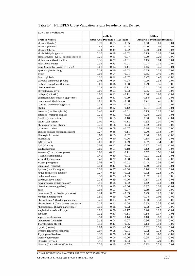
USING REGRESSION ANALYSES FOR THE DETERMINATION
OF PROTEIN STRUCTURE FROM FTIR SPECTRA 217
Table B4. FTIR/PLS Cross-Validation results for α-helix, and β-sheet
PLS Cross-Validation
α-Helix β-Sheet
Protein Names Observed Predicted Residual Observed PredictedResidual
albumin (bovine) 0.70 0.75 -0.05 0.00 -0.01 0.01
albumin (human) 0.69 0.61 0.08 0.00 0.01 -0.01
albumin (sheep) 0.71 0.49 0.22 0.00 0.04 -0.04
alcohol dehydrogenase 0.16 0.18 -0.02 0.19 0.18 0.01
alpha amylase_type2 (basillus species) 0.20 0.13 0.07 0.29 0.29 0.00
alpha casein (bovine milk) 0.36 0.37 -0.01 0.15 0.14 0.01
alpha_lactalbumin 0.32 0.33 -0.01 0.07 0.11 -0.04
apha-Crystallin(Bovine eye lens) 0.03 0.14 -0.11 0.46 0.45 0.01
aprotinin (bovine lung) 0.14 0.16 -0.02 0.25 0.22 0.03
avidin 0.03 0.04 -0.01 0.55 0.49 0.06
B-lactoglobulin 0.10 0.12 -0.02 0.42 0.45 -0.03
carbonic anhydrase (bovin) 0.08 0.16 -0.08 0.29 0.33 -0.04
carbonic anhydrase (human) 0.08 0.16 -0.08 0.29 0.35 -0.06
choline oxidase 0.21 0.10 0.11 0.21 0.26 -0.05
chymotrypsin(bovin) 0.00 0.03 -0.03 0.35 0.38 -0.03
collagen(calf skin) 0.00 0.11 -0.11 0.00 0.07 -0.07
conalbumin.dpt(chicken egg white) 0.28 0.37 -0.09 0.18 0.15 0.03
concanavalin(jack bean) 0.00 0.08 -0.08 0.41 0.46 -0.05
d_amino acid dehydrogenase 0.18 0.10 0.08 0.27 0.20 0.07
elastin 0.00 0.12 -0.12 0.31 0.32 -0.01
esterase (bacillus sybstilis) 0.40 0.41 -0.01 0.15 0.12 0.03
esterase (rhizopus oryzae) 0.25 0.22 0.03 0.28 0.29 -0.01
ferritin (horse spleen) 0.75 0.65 0.10 0.00 0.01 -0.01
fetuin (calf serum) 0.00 0.11 -0.11 0.32 0.30 0.02
fibrinogen(bovine plasma) 0.70 0.66 0.04 0.02 0.00 0.02
galactose oxidase 0.01 0.08 -0.07 0.38 0.38 0.00
glucose oxidase (aspegillus niger) 0.27 0.38 -0.11 0.20 0.13 0.07
Hemoglobin bovine 0.67 0.65 0.02 0.00 0.03 -0.03
hexakinase 0.44 0.50 -0.06 0.15 0.18 -0.03
IgG (bovine) 0.08 -0.01 0.09 0.37 0.34 0.03
IgG (Human) 0.08 -0.12 0.20 0.37 0.40 -0.03
insulin (human) 0.69 0.51 0.18 0.12 0.08 0.04
invertase(from bakers yeast) 0.00 -0.11 0.11 0.57 0.56 0.01
l_lactic (rabbit muscle) 0.40 0.39 0.01 0.21 0.22 -0.01
lactic dehydrogenase 0.45 0.37 0.08 0.20 0.25 -0.05
lectin ( p.vulgaris) 0.02 0.03 -0.01 0.43 0.36 0.07
lglutathion (reduced) 0.51 0.47 0.04 0.09 0.10 -0.01
lipaseA (candida rugosa) 0.33 0.37 -0.04 0.14 0.13 0.01
native form of c1 inhibitor 0.27 0.29 -0.02 0.32 0.23 0.09
native ovalbumin 0.30 0.35 -0.05 0.32 0.26 0.06
papain(papaya lanex) 0.23 0.29 -0.06 0.17 0.14 0.03
pepsin(pepsin gastric mucosa) 0.10 0.08 0.02 0.42 0.41 0.01
phosvitin(from egg white) 0.29 0.35 -0.06 0.37 0.38 -0.01
porin 0.04 -0.03 0.07 0.59 0.59 0.00
proteinase (from bovine pancreas) 0.24 0.27 -0.03 0.23 0.23 0.00
rhodopsin unbleached 0.59 0.59 0.00 0.04 0.06 -0.02
ribonucleaus A (bovine pancrease) 0.20 0.13 0.07 0.30 0.30 0.00
ribonucleaus S (from bovine pancreas) 0.19 0.11 0.08 0.33 0.35 -0.02
ribonucleausB (bovine pancrease) 0.18 0.16 0.02 0.33 0.27 0.06
staphylokinase-B wild type 0.09 0.26 -0.17 0.28 0.29 -0.01
subtilisin 0.32 0.43 -0.11 0.18 0.17 0.01
superoxide dismutase 0.51 0.37 0.14 0.10 0.18 -0.08
thaumactin (t.danielli) 0.11 0.04 0.07 0.36 0.36 0.00
Transketalose (E.coli) 0.42 0.47 -0.05 0.14 0.12 0.02
trypsin (bovine) 0.07 0.13 -0.06 0.32 0.31 0.01
trypsinogen(bovine pancreas) 0.07 0.08 -0.01 0.32 0.34 -0.02
Tryptophan Synthase 0.32 0.38 -0.06 0.06 0.08 -0.02
typsin-chymotripsin 0.00 0.06 -0.06 0.25 0.30 -0.05
ubiquitin (bovine) 0.16 0.20 -0.04 0.31 0.29 0.02
Urease (Canavalia ensiformis) 0.26 0.19 0.07 0.22 0.21 0.01

APPENDIX
218
Table B5. FTIR/PLS Cross-Validation results for parallel β-sheet, antiparallel β-sheet and
mixed β-sheet
PLS Cross-Validation
Parallel β-Sheet antiParallel β-Sheet mixed β-Sheet
PDBID Protein Names Observed Predicted Residual Observed Predicted Residual Observed Predicted Residual
3V03 albumin (bovine) 0.00 0.02 -0.02 0.00 0.00 0.00 0.00 0.00 0.00
1A06 albumin (human) 0.00 0.02 -0.02 0.00 -0.02 0.02 0.00 0.00 0.00
1E7H albumin (sheep) 0.00 0.02 -0.02 0.00 0.03 -0.03 0.00 -0.01 0.01
6ADH alcohol dehydrogenase 0.07 0.06 0.01 0.11 0.11 0.00 0.01 0.01 0.00
1QHO alpha amylase_type2 (basillus species) 0.06 0.08 -0.02 0.20 0.20 0.00 0.01 0.01 0.00
1DAY alpha casein (bovine milk) 0.00 0.01 -0.01 0.13 0.11 0.02 0.00 0.00 0.00
1HFZ alpha_lactalbumin 0.00 0.03 -0.03 0.07 0.11 -0.04 0.00 0.00 0.00
4GCR apha-Crystallin(Bovine eye lens) 0.00 0.00 0.00 0.38 0.40 -0.02 0.00 0.00 0.00
3LDJ aprotinin (bovine lung) 0.00 0.01 -0.01 0.25 0.23 0.02 0.00 -0.01 0.01
1SLF avidin 0.00 0.01 -0.01 0.53 0.45 0.08 0.00 0.01 -0.01
1BEB B-lactoglobulin 0.00 0.00 0.00 0.38 0.41 -0.03 0.00 -0.01 0.01
1V9E carbonic anhydrase (bovin) 0.04 0.01 0.03 0.19 0.27 -0.08 0.05 0.03 0.02
3M1K carbonic anhydrase (human) 0.04 0.01 0.03 0.19 0.29 -0.10 0.05 0.03 0.02
3NNE choline oxidase 0.06 0.04 0.02 0.12 0.18 -0.06 0.01 0.00 0.01
1YPH chymotrypsin(bovin) 0.00 0.02 -0.02 0.32 0.30 0.02 0.00 0.01 -0.01
1BKV collagen(calf skin) 0.00 0.03 -0.03 0.00 0.05 -0.05 0.00 0.00 0.00
1OVT conalbumin.dpt(chicken egg white) 0.06 0.03 0.03 0.11 0.10 0.01 0.00 0.00 0.00
3CNA concanavalin(jack bean) 0.00 0.04 -0.04 0.41 0.43 -0.02 0.00 0.00 0.00
1MPX d_amino acid dehydrogenase 0.06 0.03 0.03 0.18 0.13 0.05 0.01 0.01 0.00
2OII elastin 0.00 0.03 -0.03 0.29 0.30 -0.01 0.00 0.00 0.00
1W17 esterase (bacillus sybstilis) 0.13 0.03 0.10 0.02 0.04 -0.02 0.00 0.00 0.00
1T1C esterase (rhizopus oryzae) 0.00 0.04 -0.04 0.27 0.26 0.01 0.00 0.00 0.00
3F32 ferritin (horse spleen) 0.00 0.01 -0.01 0.00 0.00 0.00 0.00 0.00 0.00
1DLP fetuin (calf serum) 0.00 -0.01 0.01 0.31 0.29 0.02 0.00 0.00 0.00
3GHG fibrinogen(bovine plasma) 0.00 0.03 -0.03 0.01 0.00 0.01 0.01 0.00 0.01
2EIB galactose oxidase 0.01 -0.03 0.04 0.34 0.35 -0.01 0.01 0.01 0.00
1GAL glucose oxidase (aspegillus niger) 0.05 0.02 0.03 0.12 0.09 0.03 0.01 0.01 0.00
2QSP Hemoglobin bovine 0.00 0.03 -0.03 0.00 -0.01 0.01 0.00 0.01 -0.01
1BG3 hexakinase 0.05 0.04 0.01 0.08 0.11 -0.03 0.02 0.02 0.00
1IGT IgG (bovine) 0.00 0.01 -0.01 0.37 0.32 0.05 0.00 0.01 -0.01
3AGV IgG (Human) 0.00 0.00 0.00 0.37 0.39 -0.02 0.00 0.01 -0.01
2OLY insulin (human) 0.00 0.01 -0.01 0.12 0.08 0.04 0.00 0.00 0.00
1W2T invertase(from bakers yeast) 0.01 0.01 0.00 0.49 0.47 0.02 0.00 0.00 0.00
3H3F l_lactic (rabbit muscle) 0.08 0.02 0.06 0.11 0.17 -0.06 0.00 0.00 0.00
1LDM lactic dehydrogenase 0.08 0.05 0.03 0.11 0.15 -0.04 0.00 0.01 -0.01
1IOA lectin ( p.vulgaris) 0.00 0.01 -0.01 0.43 0.33 0.10 0.00 0.01 -0.01
1HNA lglutathion (reduced) 0.04 0.02 0.02 0.04 0.04 0.00 0.01 0.02 -0.01
1CRL lipaseA (candida rugosa) 0.06 0.04 0.02 0.05 0.04 0.01 0.01 0.01 0.00
2OAY native form of c1 inhibitor 0.01 0.01 0.00 0.28 0.24 0.04 0.01 0.00 0.01
1OVA native ovalbumin 0.03 0.04 -0.01 0.22 0.14 0.08 0.05 0.04 0.01
9PAP papain(papaya lanex) 0.01 0.05 -0.04 0.15 0.11 0.04 0.01 0.00 0.01
1YX9 pepsin(pepsin gastric mucosa) 0.04 0.02 0.02 0.32 0.33 -0.01 0.03 0.03 0.00
1LSH phosvitin(from egg white) 0.00 0.02 -0.02 0.35 0.34 0.01 0.00 0.01 -0.01
2ZFG porin 0.00 0.01 -0.01 0.56 0.57 -0.01 0.00 0.00 0.00
3AJ8 proteinase (from bovine pancreas) 0.14 0.11 0.03 0.08 0.09 -0.01 0.01 0.01 0.00
1HZX rhodopsin unbleached 0.00 0.03 -0.03 0.04 0.04 0.00 0.00 -0.01 0.01
1RBX ribonucleaus A (bovine pancrease) 0.00 0.01 -0.01 0.28 0.28 0.00 0.01 0.02 -0.01
3DJV ribonucleaus S (from bovine pancreas) 0.00 0.01 -0.01 0.31 0.32 -0.01 0.01 0.01 0.00
1RBB ribonucleausB (bovine pancrease) 0.00 0.01 -0.01 0.31 0.25 0.06 0.01 0.02 -0.01
1SSN staphylokinase-B wild type 0.07 0.03 0.04 0.14 0.15 -0.01 0.06 0.06 0.00
1GNS subtilisin 0.13 0.04 0.09 0.04 0.06 -0.02 0.00 0.01 -0.01
3CEI superoxide dismutase 0.00 0.02 -0.02 0.09 0.13 -0.04 0.00 0.01 -0.01
1RQW thaumactin (t.danielli) 0.00 0.01 -0.01 0.27 0.27 0.00 0.05 0.05 0.00
1QGD Transketalose (E.coli) 0.11 0.11 0.00 0.02 -0.01 0.03 0.00 0.00 0.00
3A7T trypsin (bovine) 0.00 0.03 -0.03 0.30 0.30 0.00 0.00 0.00 0.00
2TGA trypsinogen(bovine pancreas) 0.00 0.00 0.00 0.30 0.33 -0.03 0.00 0.00 0.00
2J9Z Tryptophan Synthase 0.00 0.01 -0.01 0.06 0.06 0.00 0.00 0.01 -0.01
1BBI typsin-chymotripsin 0.00 0.01 -0.01 0.25 0.29 -0.04 0.00 0.01 -0.01
2ZCB ubiquitin (bovine) 0.03 0.01 0.02 0.23 0.23 0.00 0.05 0.03 0.02
4H9M Urease (Canavalia ensiformis) 0.07 0.08 -0.01 0.13 0.11 0.02 0.01 0.01 0.00

USING REGRESSION ANALYSES FOR THE DETERMINATION
OF PROTEIN STRUCTURE FROM FTIR SPECTRA 219
Table B6. FTIR/PLS Cross-Validation results for 310-helix, turns and other
PLS Cross-Validation
310 helix β-turns Other
PDBID Protein Names Observed Predicted Residual Observed Predicted Residual Observed Predicted Residual
3V03 albumin (bovine) 0.04 0.03 0.01 0.09 0.11 -0.02 0.16 0.13 0.03
1A06 albumin (human) 0.02 0.03 -0.01 0.09 0.09 0.00 0.19 0.25 -0.06
1E7H albumin (sheep) 0.02 0.04 -0.02 0.09 0.08 0.01 0.17 0.30 -0.13
6ADH alcohol dehydrogenase 0.02 0.00 0.02 0.18 0.17 0.01 0.45 0.43 0.02
1QHO alpha amylase_type2 (basillus species) 0.03 0.05 -0.02 0.14 0.14 0.00 0.34 0.32 0.02
1DAY alpha casein (bovine milk) 0.08 0.06 0.02 0.10 0.10 0.00 0.31 0.30 0.01
1HFZ alpha_lactalbumin 0.14 0.08 0.06 0.17 0.14 0.03 0.31 0.29 0.02
4GCR apha-Crystallin(Bovine eye lens) 0.06 0.05 0.01 0.08 0.08 0.00 0.37 0.31 0.06
3LDJ aprotinin (bovine lung) 0.07 0.04 0.03 0.07 0.07 0.00 0.46 0.40 0.06
1SLF avidin 0.05 0.05 0.00 0.05 0.09 -0.04 0.32 0.34 -0.02
1BEB B-lactoglobulin 0.06 0.05 0.01 0.12 0.12 0.00 0.29 0.28 0.01
1V9E carbonic anhydrase (bovin) 0.08 0.06 0.02 0.11 0.11 0.00 0.44 0.37 0.07
3M1K carbonic anhydrase (human) 0.08 0.05 0.03 0.11 0.12 -0.01 0.44 0.33 0.11
3NNE choline oxidase 0.05 0.06 -0.01 0.14 0.15 -0.01 0.40 0.38 0.02
1YPH chymotrypsin(bovin) 0.02 0.04 -0.02 0.18 0.14 0.04 0.45 0.40 0.05
1BKV collagen(calf skin) 0.00 0.02 -0.02 0.00 0.03 -0.03 1.00 0.71 0.29
1OVT conalbumin.dpt(chicken egg white) 0.05 0.04 0.01 0.16 0.11 0.05 0.34 0.34 0.00
3CNA concanavalin(jack bean) 0.00 0.02 -0.02 0.09 0.10 -0.01 0.50 0.42 0.08
1MPX d_amino acid dehydrogenase 0.05 0.04 0.01 0.12 0.09 0.03 0.38 0.61 -0.23
2OII elastin 0.00 0.01 -0.01 0.08 0.05 0.03 0.61 0.55 0.06
1W17 esterase (bacillus sybstilis) 0.03 0.05 -0.02 0.10 0.10 0.00 0.32 0.31 0.01
1T1C esterase (rhizopus oryzae) 0.02 0.01 0.01 0.14 0.14 0.00 0.31 0.30 0.01
3F32 ferritin (horse spleen) 0.00 0.04 -0.04 0.07 0.08 -0.01 0.19 0.22 -0.03
1DLP fetuin (calf serum) 0.00 0.00 0.00 0.09 0.05 0.04 0.58 0.62 -0.04
3GHG fibrinogen(bovine plasma) 0.02 0.02 0.00 0.06 0.09 -0.03 0.21 0.26 -0.05
2EIB galactose oxidase 0.02 0.03 -0.01 0.13 0.14 -0.01 0.46 0.47 -0.01
1GAL glucose oxidase (aspegillus niger) 0.07 0.07 0.00 0.12 0.10 0.02 0.33 0.31 0.02
2QSP Hemoglobin bovine 0.09 0.08 0.01 0.11 0.12 -0.01 0.14 0.21 -0.07
1BG3 hexakinase 0.03 0.00 0.03 0.11 0.11 0.00 0.27 0.15 0.12
1IGT IgG (bovine) 0.04 0.07 -0.03 0.08 0.10 -0.02 0.42 0.44 -0.02
3AGV IgG (Human) 0.04 0.02 0.02 0.08 0.07 0.01 0.42 0.51 -0.09
2OLY insulin (human) 0.12 0.06 0.06 0.00 0.08 -0.08 0.08 0.27 -0.19
1W2T invertase(from bakers yeast) 0.03 0.02 0.01 0.10 0.10 0.00 0.30 0.43 -0.13
3H3F l_lactic (rabbit muscle) 0.04 0.05 -0.01 0.11 0.11 0.00 0.24 0.26 -0.02
1LDM lactic dehydrogenase 0.07 0.05 0.02 0.06 0.05 0.01 0.22 0.32 -0.10
1IOA lectin ( p.vulgaris) 0.04 0.05 -0.01 0.14 0.12 0.02 0.37 0.41 -0.04
1HNA lglutathion (reduced) 0.03 0.07 -0.04 0.12 0.10 0.02 0.26 0.27 -0.01
1CRL lipaseA (candida rugosa) 0.05 0.05 0.00 0.13 0.16 -0.03 0.36 0.45 -0.09
2OAY native form of c1 inhibitor 0.02 0.04 -0.02 0.09 0.10 -0.01 0.30 0.31 -0.01
1OVA native ovalbumin 0.03 0.05 -0.02 0.13 0.14 -0.01 0.23 0.28 -0.05
9PAP papain(papaya lanex) 0.03 0.03 0.00 0.11 0.12 -0.01 0.46 0.42 0.04
1YX9 pepsin(pepsin gastric mucosa) 0.04 0.06 -0.02 0.13 0.14 -0.01 0.31 0.30 0.01
1LSH phosvitin(from egg white) 0.02 0.02 0.00 0.10 0.09 0.01 0.23 0.13 0.10
2ZFG porin 0.00 -0.01 0.01 0.14 0.12 0.02 0.24 0.33 -0.09
3AJ8 proteinase (from bovine pancreas) 0.03 0.01 0.02 0.16 0.20 -0.04 0.34 0.44 -0.10
1HZX rhodopsin unbleached 0.03 0.04 -0.01 0.10 0.11 -0.01 0.25 0.23 0.02
1RBX ribonucleaus A (bovine pancrease) 0.02 0.03 -0.01 0.06 0.09 -0.03 0.41 0.43 -0.02
3DJV ribonucleaus S (from bovine pancreas) 0.05 0.05 0.00 0.11 0.13 -0.02 0.32 0.38 -0.06
1RBB ribonucleausB (bovine pancrease) 0.03 0.04 -0.01 0.15 0.13 0.02 0.31 0.37 -0.06
1SSN staphylokinase-B wild type 0.02 0.02 0.00 0.08 0.09 -0.01 0.53 0.37 0.16
1GNS subtilisin 0.00 0.01 -0.01 0.16 0.12 0.04 0.34 0.32 0.02
3CEI superoxide dismutase 0.03 0.04 -0.01 0.13 0.12 0.01 0.23 0.28 -0.05
1RQW thaumactin (t.danielli) 0.01 0.04 -0.03 0.12 0.12 0.00 0.40 0.41 -0.01
1QGD Transketalose (E.coli) 0.05 0.06 -0.01 0.13 0.15 -0.02 0.26 0.15 0.11
3A7T trypsin (bovine) 0.03 0.02 0.01 0.15 0.16 -0.01 0.43 0.41 0.02
2TGA trypsinogen(bovine pancreas) 0.03 0.02 0.01 0.14 0.16 -0.02 0.44 0.46 -0.02
2J9Z Tryptophan Synthase 0.10 0.08 0.02 0.24 0.16 0.08 0.28 0.26 0.02
1BBI typsin-chymotripsin 0.00 0.04 -0.04 0.06 0.13 -0.07 0.69 0.41 0.28
2ZCB ubiquitin (bovine) 0.08 0.06 0.02 0.16 0.11 0.05 0.28 0.33 -0.05
4H9M Urease (Canavalia ensiformis) 0.04 0.03 0.01 0.15 0.14 0.01 0.34 0.37 -0.03

APPENDIX
220
Table B7. Result of 44 samples in the test set used for Partial Least Squares (PLS)
analysis. About 20 spectra from calibration set were included in the test set for validation
purpose (α-helix and β-sheet only).
α-Helix β-Sheet
PDBID Protein Names Observed Predicted Residual Observed Predicted Residual
1E7H albumin (sheep) 0.71 0.49 0.22 0.00 0.04 -0.04
1DAY alpha casein (bovine milk) 0.36 0.37 -0.01 0.15 0.14 0.01
1HFZ alpha_lactalbumin 0.31 0.33 -0.02 0.07 0.11 -0.04
3CWL alpha-1-antitypsin 0.28 0.18 0.10 0.31 0.33 -0.02
1YJ0 annexinV/without calcium 0.68 0.53 0.15 0.00 0.08 -0.08
1AS4 anti-chymotrypsin 0.32 0.25 0.07 0.37 0.30 0.07
3LDJ aprotinin (bovine lung) 0.14 0.16 -0.02 0.25 0.22 0.03
1SLF avidin 0.03 0.04 -0.01 0.55 0.49 0.06
2BRD bacteriorhodopsin in purple membrane 0.77 0.35 0.42 0.00 0.20 -0.20
3IF7 calmodulin 0.59 0.51 0.08 0.06 0.08 -0.02
3M1K carbonic anhydrase (human) 0.08 0.16 -0.08 0.29 0.33 -0.04
1YPH chymotrypsin(bovin) 0.00 0.03 -0.03 0.35 0.38 -0.03
1ATH cleaved form of anti-thrombin 0.27 0.28 -0.01 0.32 0.30 0.02
1BKV collagen(calf skin) 0.00 0.11 -0.11 0.00 0.07 -0.07
1HRC cytochrome (horse heart) 0.41 0.49 -0.08 0.00 0.02 -0.02
1GAL glucose oxidase (aspegillus niger) 0.27 0.38 -0.11 0.20 0.13 0.07
1IGT IgG (bovine) 0.06 -0.01 0.07 0.42 0.34 0.08
2OLY insulin (human) 0.69 0.51 0.18 0.12 0.08 0.04
3H3F l_lactic (rabbit muscle) 0.40 0.39 0.01 0.21 0.22 -0.01
1IOA lectin ( p.vulgaris) 0.02 0.03 -0.01 0.43 0.36 0.07
1HNA l-glutathion (reduced) 0.51 0.47 0.04 0.09 0.10 -0.01
1OIL lipase (wheat) 0.36 0.34 0.02 0.18 0.19 -0.01
2LYZ lysozyme (chicken egg) 0.32 0.40 -0.08 0.06 0.12 -0.06
2MLT melittin pH 6 0.88 0.47 0.41 0.00 0.12 -0.12
1NZ2 myoglobulin(horse muscle) 0.74 0.62 0.12 0.00 0.01 -0.01
3DLW native anti-chymotrypsin 0.29 0.29 0.00 0.36 0.25 0.11
1T1F native form of anti-thrombin 0.26 0.27 -0.01 0.27 0.32 -0.05
1OVA native ovalbumin 0.30 0.35 -0.05 0.32 0.26 0.06
1HCH peroxidase (horseradish) 0.44 0.35 0.09 0.02 0.17 -0.15
2AXT phtosystem II reaction centre 0.52 0.50 0.02 0.01 0.12 -0.11
3ENJ pig citrate synthase 0.59 0.49 0.10 0.03 0.10 -0.07
1T5A pyruvate kinase 0.36 0.51 -0.15 0.20 0.11 0.09
1QOV Reaction centere R. Sphae. 0.18 0.38 -0.20 0.22 0.21 0.01
2I37 rhodopsin bleached 0.55 0.61 -0.06 0.04 0.03 0.01
1HZX rhodopsin unbleached 0.59 0.59 0.00 0.04 0.06 -0.02
2ACH sact1 DIFF 0.31 0.25 0.06 0.34 0.30 0.04
1LQ8 split form of c1 inhibitor 0.28 0.29 -0.01 0.35 0.25 0.10
1H3E split form ovalbumin 0.41 0.35 0.06 0.13 0.27 -0.14
3CEI superoxide dismutase 0.51 0.37 0.14 0.10 0.18 -0.08
1RQW thaumactin (t.danielli) 0.11 0.04 0.07 0.36 0.36 0.00
3A7T trypsin 0.07 0.22 -0.15 0.32 0.27 0.05
1UHB trypsin (hog pancreas) 0.00 0.01 -0.01 0.34 0.40 -0.06
2J9Z tryptophan Synthase 0.32 0.38 -0.06 0.06 0.08 -0.02
2ZCB ubiquitin (bovine) 0.16 0.20 -0.04 0.31 0.29 0.02

USING REGRESSION ANALYSES FOR THE DETERMINATION
OF PROTEIN STRUCTURE FROM FTIR SPECTRA 221
Table B8. Result of 44 samples in the test set used for Partial Least Squares (PLS)
analysis. About 20 spectra from calibration set were included in the test set for validation
purpose (parallel β-sheet, parallel β-sheet, and mixed β-sheet).
PDBID Protein Names Observed Predicted Residual Observed Predicted Residual Observed Predicted Residual
1E7H albumin (sheep) 0.00 0.02 -0.02 0.00 0.02 -0.02 0.00 0.00 0.00
1DAY alpha casein (bovine milk) 0.00 0.01 -0.01 0.13 0.11 0.02 0.00 0.01 -0.01
1HFZ alpha_lactalbumin 0.00 0.03 -0.03 0.07 0.11 -0.04 0.00 0.00 0.00
3CWL alpha-1-antitypsin' 0.03 0.33 -0.30 0.21 0.21 0.27 0.06 0.02 0.04
1YJ0 annexinV/without calcium 0.00 0.03 -0.03 0.00 0.04 -0.04 0.00 0.01 -0.01
1AS4 anti-chymotrypsin 0.02 0.02 0.00 0.32 0.25 0.07 0.02 0.02 0.00
3LDJ aprotinin (bovine lung) 0.00 0.01 -0.01 0.25 0.22 0.03 0.00 -0.01 0.01
1SLF avidin 0.00 0.01 -0.01 0.53 0.45 0.08 0.00 0.01 -0.01
2BRD bacteriorhodopsin in purple membrane 0.00 0.02 -0.02 0.00 0.18 -0.18 0.00 0.01 -0.01
3IF7 calmodulin 0.00 0.03 -0.03 0.06 0.05 0.01 0.00 0.01 -0.01
3M1K carbonic anhydrase (human) 0.04 0.01 0.03 0.19 0.27 -0.08 0.05 0.02 0.03
1YPH chymotrypsin(bovin) 0.00 0.02 -0.02 0.32 0.30 0.02 0.00 0.01 -0.01
1ATH cleaved form of anti-thrombin 0.03 0.02 0.01 0.25 0.26 -0.01 0.03 0.01 0.02
1BKV collagen(calf skin) 0.00 0.03 -0.03 0.00 0.06 -0.06 0.00 -0.01 0.01
1HRC cytochrome (horse heart) 0.00 0.02 -0.02 0.00 0.01 -0.01 0.00 0.00 0.00
1GAL glucose oxidase (aspegillus niger) 0.05 0.02 0.03 0.12 0.09 0.03 0.01 0.01 0.00
1IGT IgG (bovine) 0.00 0.01 -0.01 0.42 0.32 0.10 0.00 0.02 -0.02
2OLY insulin (human) 0.00 0.01 -0.01 0.12 0.07 0.05 0.00 0.01 -0.01
3H3F l_lactic (rabbit muscle) 0.08 0.02 0.06 0.11 0.15 -0.04 0.00 0.01 -0.01
1IOA lectin ( p.vulgaris) 0.00 0.01 -0.01 0.43 0.32 0.11 0.00 0.01 -0.01
1HNA lglutathion (reduced) 0.04 0.02 0.02 0.04 0.05 -0.01 0.01 0.02 -0.01
1OIL lipase (wheat) 0.09 0.02 0.07 0.07 0.14 -0.07 0.00 0.01 -0.01
2LYZ lysozyme (chicken egg) 0.00 0.02 -0.02 0.06 0.09 -0.03 0.00 0.01 -0.01
2MLT melittin pH 6 0.00 0.03 -0.03 0.00 0.07 -0.07 0.00 0.01 -0.01
1NZ2 myoglobulin(horse muscle) 0.00 0.02 -0.02 0.00 -0.03 0.03 0.00 0.00 0.00
3DLW native anti-chymotrypsin 0.02 0.02 0.00 0.31 0.19 0.12 0.02 0.02 0.00
1T1F native form of anti-thrombin 0.03 0.03 0.00 0.21 0.24 -0.03 0.03 0.02 0.01
1OVA native ovalbumin 0.03 0.04 -0.01 0.22 0.13 0.09 0.05 0.03 0.02
1HCH peroxidase (horseradish) 0.00 0.02 -0.02 0.02 0.13 -0.11 0.00 0.01 -0.01
2AXT phtosystem II reaction centre 0.01 0.02 -0.01 0.00 0.11 -0.11 0.00 0.01 -0.01
3ENJ pig citrate synthase 0.00 0.03 -0.03 0.03 0.07 -0.04 0.00 0.01 -0.01
1T5A pyruvate kinase 0.10 0.02 0.08 0.08 0.09 -0.01 0.01 0.01 0.00
1QOV Reaction centere R. Sphae. 0.00 0.02 -0.02 0.18 0.17 0.01 0.02 0.01 0.01
2I37 rhodopsin bleached 0.00 0.03 -0.03 0.04 0.01 0.03 0.00 0.01 -0.01
1HZX rhodopsin unbleached 0.00 0.03 -0.03 0.04 0.04 0.00 0.00 0.00 0.00
2ACH sact1 DIFF 0.02 0.02 0.00 0.29 0.25 0.04 0.02 0.02 0.00
1LQ8 split form of c1 inhibitor 0.02 0.01 0.01 0.30 0.25 0.05 0.02 0.01 0.01
1H3E split form ovalbumin 0.07 0.04 0.03 0.05 0.12 -0.07 0.01 0.03 -0.02
3CEI superoxide dismutase 0.00 0.02 -0.02 0.09 0.14 -0.05 0.00 0.01 -0.01
1RQW thaumactin (t.danielli) 0.00 0.01 -0.01 0.27 0.27 0.00 0.05 0.02 0.03
3A7T trypsin 0.00 0.03 -0.03 0.30 0.20 0.10 0.00 0.02 -0.02
1UHB trypsin (hog pancreas) 0.00 0.02 -0.02 0.33 0.32 0.01 0.00 0.02 -0.02
2J9Z tryptophan Synthase 0.00 0.01 -0.01 0.06 0.07 -0.01 0.00 0.02 -0.02
2ZCB ubiquitin (bovine) 0.03 0.01 0.02 0.23 0.23 0.00 0.05 0.02 0.03

APPENDIX
222
Table B9. Result of 44 samples in the test set used for Partial Least Squares (PLS)
analysis. About 20 spectra from calibration set were included in the test set for validation
purpose (310-helix, β-turns and other).
PDBID Protein Names Observed Predicted Residual Observed Predicted Residual Observed Predicted Residual
1E7H albumin (sheep) 0.02 0.04 -0.02 0.09 0.08 0.01 0.17 0.30 -0.13
1DAY alpha casein (bovine milk) 0.08 0.06 0.02 0.10 0.10 0.00 0.31 0.30 0.01
1HFZ alpha_lactalbumin 0.14 0.07 0.07 0.18 0.14 0.04 0.31 0.29 0.02
3CWL alpha-1-antitypsin' 0.02 0.04 -0.02 0.10 0.12 -0.02 0.28 0.35 -0.07
1YJ0 annexinV/without calcium 0.10 0.04 0.06 0.07 0.12 -0.05 0.25 0.25 0.00
1AS4 anti-chymotrypsin 0.02 0.04 -0.02 0.09 0.12 -0.03 0.20 0.31 -0.11
3LDJ aprotinin (bovine lung) 0.07 0.04 0.03 0.07 0.07 0.00 0.46 0.40 0.06
1SLF avidin 0.05 0.05 0.00 0.05 0.09 -0.04 0.32 0.34 -0.02
2BRD bacteriorhodopsin in purple membrane 0.00 0.04 -0.04 0.02 0.12 -0.10 0.21 0.29 -0.08
3IF7 calmodulin 0.00 0.04 -0.04 0.07 0.11 -0.04 0.28 0.25 0.03
3M1K carbonic anhydrase (human) 0.08 0.05 0.03 0.11 0.11 0.00 0.44 0.37 0.07
1YPH chymotrypsin(bovin) 0.02 0.04 -0.02 0.18 0.14 0.04 0.45 0.40 0.05
1ATH cleaved form of anti-thrombin 0.02 0.03 -0.01 0.11 0.11 0.00 0.28 0.29 -0.01
1BKV collagen(calf skin) 0.00 0.02 -0.02 0.00 0.03 -0.03 1.00 0.71 0.29
1HRC cytochrome (horse heart) 0.00 0.05 -0.05 0.17 0.10 0.07 0.41 0.29 0.12
1GAL glucose oxidase (aspegillus niger) 0.07 0.06 0.01 0.12 0.10 0.02 0.33 0.31 0.02
1IGT IgG (bovine) 0.02 0.04 -0.02 0.08 0.10 -0.02 0.42 0.44 -0.02
2OLY insulin (human) 0.12 0.06 0.06 0.00 0.08 -0.08 0.08 0.27 -0.19
3H3F l_lactic (rabbit muscle) 0.04 0.06 -0.02 0.11 0.11 0.00 0.24 0.26 -0.02
1IOA lectin ( p.vulgaris) 0.04 0.05 -0.01 0.14 0.12 0.02 0.37 0.41 -0.04
1HNA lglutathion (reduced) 0.03 0.07 -0.04 0.12 0.10 0.02 0.26 0.27 -0.01
1OIL lipase (wheat) 0.02 0.05 -0.03 0.16 0.11 0.05 0.28 0.31 -0.03
2LYZ lysozyme (chicken egg) 0.10 0.05 0.05 0.24 0.10 0.14 0.28 0.30 -0.02
2MLT melittin pH 6 0.00 0.04 -0.04 0.04 0.11 -0.07 0.08 0.26 -0.18
1NZ2 myoglobulin(horse muscle) 0.00 0.06 -0.06 0.12 0.09 0.03 0.14 0.23 -0.09
3DLW native anti-chymotrypsin 0.02 0.04 -0.02 0.07 0.12 -0.05 0.27 0.31 -0.04
1T1F native form of anti-thrombin 0.04 0.03 0.01 0.10 0.12 -0.02 0.33 0.30 0.03
1OVA native ovalbumin 0.03 0.04 -0.01 0.13 0.14 -0.01 0.23 0.28 -0.05
1HCH peroxidase (horseradish) 0.06 0.05 0.01 0.17 0.10 0.07 0.31 0.31 0.00
2AXT phtosystem II reaction centre 0.04 0.04 0.00 0.10 0.11 -0.01 0.33 0.24 0.09
3ENJ pig citrate synthase 0.03 0.04 -0.01 0.10 0.12 -0.02 0.24 0.25 -0.01
1T5A pyruvate kinase 0.04 0.04 0.00 0.10 0.10 0.00 0.30 0.24 0.06
1QOV Reaction centere R. Sphae. 0.06 0.04 0.02 0.12 0.12 0.00 0.42 0.27 0.15
2I37 rhodopsin bleached 0.04 0.03 0.01 0.12 0.11 0.01 0.25 0.23 0.02
1HZX rhodopsin unbleached 0.03 0.04 -0.01 0.10 0.11 -0.01 0.25 0.23 0.02
2ACH sact1 DIFF 0.02 0.04 -0.02 0.09 0.12 -0.03 0.23 0.31 -0.08
1LQ8 split form of c1 inhibitor 0.04 0.03 0.01 0.08 0.11 -0.03 0.26 0.31 -0.05
1H3E split form ovalbumin 0.04 0.04 0.00 0.14 0.14 0.00 0.28 0.29 -0.01
3CEI superoxide dismutase 0.03 0.04 -0.01 0.13 0.12 0.01 0.23 0.28 -0.05
1RQW thaumactin (t.danielli) 0.01 0.04 -0.03 0.12 0.12 0.00 0.40 0.41 -0.01
3A7T trypsin 0.03 0.04 -0.01 0.15 0.12 0.03 0.43 0.35 0.08
1UHB trypsin (hog pancreas) 0.02 0.04 -0.02 0.12 0.13 -0.01 0.51 0.42 0.09
2J9Z tryptophan Synthase 0.10 0.08 0.02 0.24 0.16 0.08 0.28 0.26 0.02
2ZCB ubiquitin (bovine) 0.08 0.06 0.02 0.16 0.11 0.05 0.28 0.33 -0.05
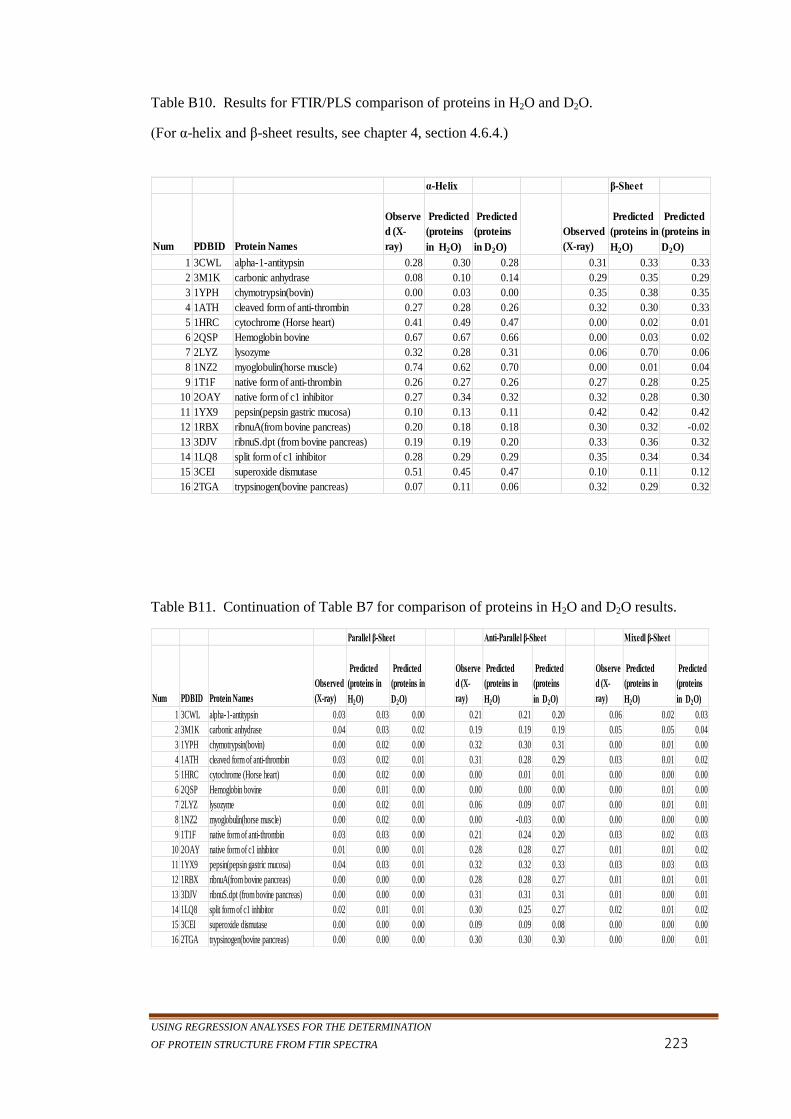
USING REGRESSION ANALYSES FOR THE DETERMINATION
OF PROTEIN STRUCTURE FROM FTIR SPECTRA 223
Table B10. Results for FTIR/PLS comparison of proteins in H2O and D2O.
(For α-helix and β-sheet results, see chapter 4, section 4.6.4.)
Table B11. Continuation of Table B7 for comparison of proteins in H2O and D2O results.
α-Helix β-Sheet
Num PDBID Protein Names
Observe
d (X-
ray)
Predicted
(proteins
in H2O)
Predicted
(proteins
in D2O)
Observed
(X-ray)
Predicted
(proteins in
H2O)
Predicted
(proteins in
D2O)
1 3CWL alpha-1-antitypsin 0.28 0.30 0.28 0.31 0.33 0.33
2 3M1K carbonic anhydrase 0.08 0.10 0.14 0.29 0.35 0.29
3 1YPH chymotrypsin(bovin) 0.00 0.03 0.00 0.35 0.38 0.35
4 1ATH cleaved form of anti-thrombin 0.27 0.28 0.26 0.32 0.30 0.33
5 1HRC cytochrome (Horse heart) 0.41 0.49 0.47 0.00 0.02 0.01
6 2QSP Hemoglobin bovine 0.67 0.67 0.66 0.00 0.03 0.02
7 2LYZ lysozyme 0.32 0.28 0.31 0.06 0.70 0.06
8 1NZ2 myoglobulin(horse muscle) 0.74 0.62 0.70 0.00 0.01 0.04
9 1T1F native form of anti-thrombin 0.26 0.27 0.26 0.27 0.28 0.25
10 2OAY native form of c1 inhibitor 0.27 0.34 0.32 0.32 0.28 0.30
11 1YX9 pepsin(pepsin gastric mucosa) 0.10 0.13 0.11 0.42 0.42 0.42
12 1RBX ribnuA(from bovine pancreas) 0.20 0.18 0.18 0.30 0.32 -0.02
13 3DJV ribnuS.dpt (from bovine pancreas) 0.19 0.19 0.20 0.33 0.36 0.32
14 1LQ8 split form of c1 inhibitor 0.28 0.29 0.29 0.35 0.34 0.34
15 3CEI superoxide dismutase 0.51 0.45 0.47 0.10 0.11 0.12
16 2TGA trypsinogen(bovine pancreas) 0.07 0.11 0.06 0.32 0.29 0.32
Parallel β-Sheet Anti-Parallel β-Sheet Mixedl β-Sheet
Num PDBID Protein Names
Observed
(X-ray)
Predicted
(proteins in
H2O)
Predicted
(proteins in
D2O)
Observe
d (X-
ray)
Predicted
(proteins in
H2O)
Predicted
(proteins
in D2O)
Observe
d (X-
ray)
Predicted
(proteins in
H2O)
Predicted
(proteins
in D2O)
1 3CWL alpha-1-antitypsin 0.03 0.03 0.00 0.21 0.21 0.20 0.06 0.02 0.03
2 3M1K carbonic anhydrase 0.04 0.03 0.02 0.19 0.19 0.19 0.05 0.05 0.04
3 1YPH chymotrypsin(bovin) 0.00 0.02 0.00 0.32 0.30 0.31 0.00 0.01 0.00
4 1ATH cleaved form of anti-thrombin 0.03 0.02 0.01 0.31 0.28 0.29 0.03 0.01 0.02
5 1HRC cytochrome (Horse heart) 0.00 0.02 0.00 0.00 0.01 0.01 0.00 0.00 0.00
6 2QSP Hemoglobin bovine 0.00 0.01 0.00 0.00 0.00 0.00 0.00 0.01 0.00
7 2LYZ lysozyme 0.00 0.02 0.01 0.06 0.09 0.07 0.00 0.01 0.01
8 1NZ2 myoglobulin(horse muscle) 0.00 0.02 0.00 0.00 -0.03 0.00 0.00 0.00 0.00
9 1T1F native form of anti-thrombin 0.03 0.03 0.00 0.21 0.24 0.20 0.03 0.02 0.03
10 2OAY native form of c1 inhibitor 0.01 0.00 0.01 0.28 0.28 0.27 0.01 0.01 0.02
11 1YX9 pepsin(pepsin gastric mucosa) 0.04 0.03 0.01 0.32 0.32 0.33 0.03 0.03 0.03
12 1RBX ribnuA(from bovine pancreas) 0.00 0.00 0.00 0.28 0.28 0.27 0.01 0.01 0.01
13 3DJV ribnuS.dpt (from bovine pancreas) 0.00 0.00 0.00 0.31 0.31 0.31 0.01 0.00 0.01
14 1LQ8 split form of c1 inhibitor 0.02 0.01 0.01 0.30 0.25 0.27 0.02 0.01 0.02
15 3CEI superoxide dismutase 0.00 0.00 0.00 0.09 0.09 0.08 0.00 0.00 0.00
16 2TGA trypsinogen(bovine pancreas) 0.00 0.00 0.00 0.30 0.30 0.30 0.00 0.00 0.01

APPENDIX
224
Table B12. Continuation of Table B8 for comparison of proteins in H2O and D2O results.
310 helix β-turns Other
Num PDBID Protein Names
Observe
d (X-
ray)
Predicted
(proteins
in H2O)
Predicted
(proteins
in D2O)
Observe
d (X-
ray)
Predicted
(proteins
in H2O)
Predicted
(proteins
in D2O)
Observe
d (X-
ray)
Predicted
(proteins in
H2O)
Predicted
(proteins
in D2O)
1 3CWL alpha-1-antitypsin 0.02 0.04 0.04 0.10 0.12 0.11 0.28 0.24 0.25
2 3M1K carbonic anhydrase 0.08 0.07 0.06 0.11 0.12 0.11 0.44 0.44 0.44
3 1YPH chymotrypsin(bovin) 0.02 0.04 0.03 0.18 0.14 0.17 0.45 0.40 0.40
4 1ATH cleaved form of anti-thrombin 0.02 0.03 0.03 0.11 0.11 0.11 0.28 0.29 0.29
5 1HRC cytochrome (Horse heart) 0.00 0.05 0.04 0.17 0.16 0.16 0.41 0.41 0.42
6 2QSP Hemoglobin bovine 0.09 0.09 0.07 0.11 0.11 0.13 0.14 0.14 0.14
7 2LYZ lysozyme 0.10 0.05 0.09 0.24 0.22 0.23 0.28 0.30 0.28
8 1NZ2 myoglobulin(horse muscle) 0.00 0.06 0.00 0.12 0.09 0.11 0.14 0.15 0.13
9 1T1F native form of anti-thrombin 0.04 0.03 0.03 0.10 0.12 0.12 0.33 0.30 0.32
10 2OAY native form of c1 inhibitor 0.02 0.02 0.02 0.09 0.08 0.08 0.30 0.30 0.30
11 1YX9 pepsin(pepsin gastric mucosa) 0.04 0.04 0.03 0.13 0.13 0.13 0.31 0.31 0.32
12 1RBX ribnuA(from bovine pancreas) 0.02 0.01 0.02 0.06 0.08 0.07 0.41 0.41 0.39
13 3DJV ribnuS.dpt (from bovine pancreas) 0.05 0.05 0.06 0.11 0.11 0.11 0.32 0.32 0.32
14 1LQ8 split form of c1 inhibitor 0.04 0.03 0.04 0.08 0.11 0.09 0.26 0.31 0.28
15 3CEI superoxide dismutase 0.03 0.04 0.04 0.13 0.14 0.14 0.23 0.23 0.23
16 2TGA trypsinogen(bovine pancreas) 0.03 0.03 0.03 0.14 0.14 0.14 0.44 0.44 0.44
USING REGRESSION ANALYSES FOR THE DETERMINATION
OF PROTEIN STRUCTURE FROM FTIR SPECTRA 225
Appendix C
Appendix C contains PCA plots for D2O and plots for Discriminant Function
Analysis (DFA) for Amide I and Amide II not used in the main body of this thesis;
the protein data set is the same and the results from these analyses were quite
favourable.
A usefulness of DFA is in maximising the differences among sample groups;
however, the score plots in the PCA analysis in Chapter 3 reviled well clustered
protein samples and served the purpose for our data exploration. See Chapter 3.

APPENDIX
226
Figure C1. Principal Component plot of Amide I region of 16 proteins in D2O showing
percentage variance of the first 4 PCs. Blue line indicates that the accumulative percentage
variance is about 98%.
Figure C2. PCA Score plot of the Amide I region for 16 proteins in D2O. The plot show
lysozyme associated with α-helix on the left. It was wrongly marked as ‘other’ before the
analysis. β-sheet proteins are clustered above right while ‘other’ appears below right.
1 2 3 40
0.1
0.2
0.3
0.4
0.5
0.6
0.7
0.8
0.9
principal comp
varia
nce e
xpla
ined (
%)
0%
10%
20%
30%
40%
50%
60%
70%
80%
90%
-4 -3 -2 -1 0 1 2-3
-2
-1
0
1
2
3
First Principal Component
Second P
rincip
al C
om
ponent
Lysozymecytochrome
Hemoglobin
myoglobulin
chymotrypsin
carbonic anhydrase
pepsinsplit-anti-thrombin
ribnuA ribnuS fewdays
nt-anti-chymotrypnative-anti-thrombin
native-c1 inhibitor
split- c1 inhibitor
trypsinogen
other
beta
alpha
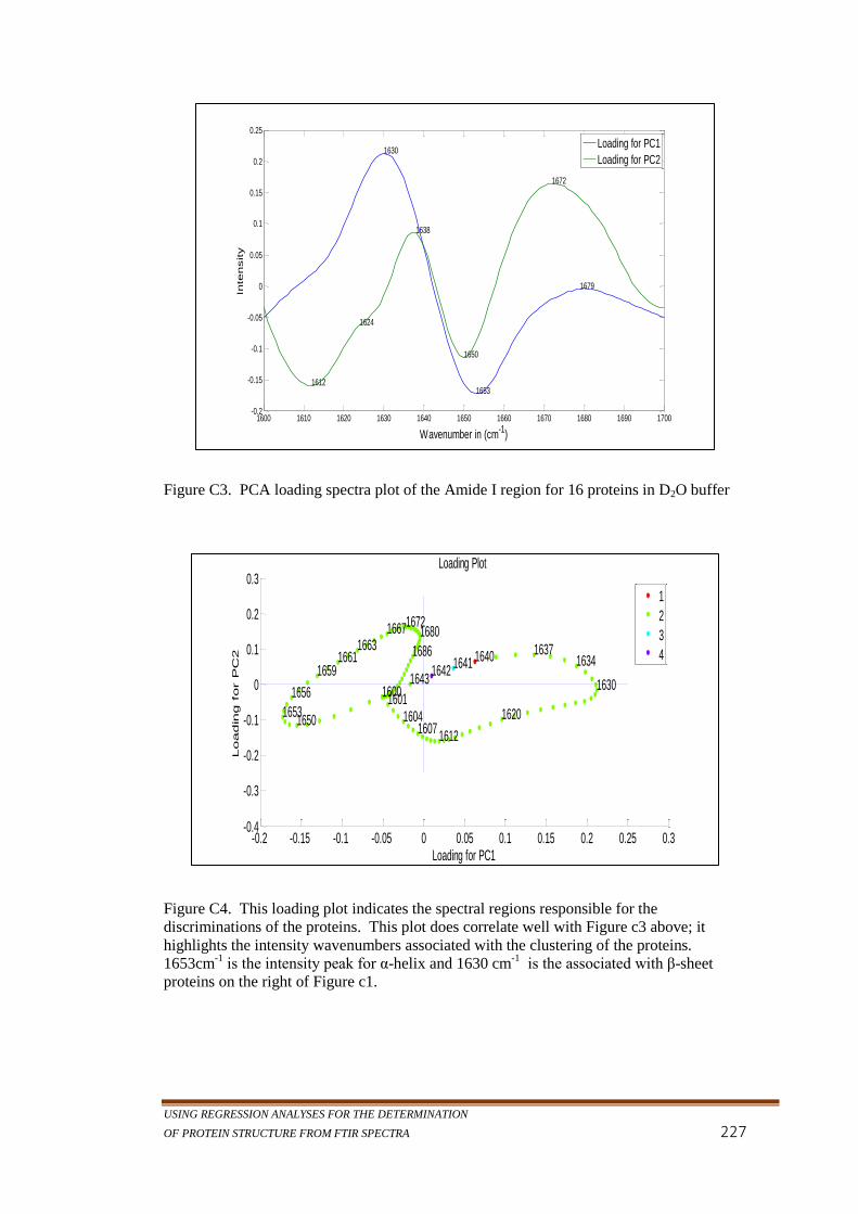
USING REGRESSION ANALYSES FOR THE DETERMINATION
OF PROTEIN STRUCTURE FROM FTIR SPECTRA 227
Figure C3. PCA loading spectra plot of the Amide I region for 16 proteins in D2O buffer
Figure C4. This loading plot indicates the spectral regions responsible for the
discriminations of the proteins. This plot does correlate well with Figure c3 above; it
highlights the intensity wavenumbers associated with the clustering of the proteins.
1653cm-1
is the intensity peak for α-helix and 1630 cm-1
is the associated with β-sheet
proteins on the right of Figure c1.
1600 1610 1620 1630 1640 1650 1660 1670 1680 1690 1700-0.2
-0.15
-0.1
-0.05
0
0.05
0.1
0.15
0.2
0.25
Wavenumber in (cm-1
)
Inte
nsity
1630
1638
1612
1624
1650
1653
1672
1679
Loading for PC1
Loading for PC2
-0.2 -0.15 -0.1 -0.05 0 0.05 0.1 0.15 0.2 0.25 0.3-0.4
-0.3
-0.2
-0.1
0
0.1
0.2
0.3
Loading for PC1
Loadin
g for P
C2
Loading Plot
16721680
16531650
1612
1630
1637164016411642
1643
16861663
16591661
1656
1667
16041607
16011600
1620
1634
1
2
3
4

APPENDIX
228
Figure C5. This plot of the Amide I region of FTIR protein spectra was produced from
Discriminant Function Analysis. The first DF discriminates between alpha-helix on the
right and beta-sheet proteins on the left; the second DF separates the ‘other’ proteins,
mainly above zero but clustered in the middle, from the rest of the data.
Figure C6. This plot of the Amide II region of FTIR protein spectra was produced from
Discriminant Function Analysis. The first DF discriminates between α-helix on the left
and β-sheet proteins on the right; the second DF separates the ‘other’ proteins, mainly
above zero but clustered in the middle, from the rest of the data.
-4 -2 0 2 4-0.4
-0.2
0
0.2
0.4
First Discriminant AnalysisSecond D
iscrim
inant
Analy
sis
other
-sheet
-helix
-3 -2 -1 0 1 2-0.4
-0.2
0
0.2
0.4
First Discriminant Analysis
Se
co
nd D
iscrim
ina
nt
An
aly
sis
other
-sheet
-helix
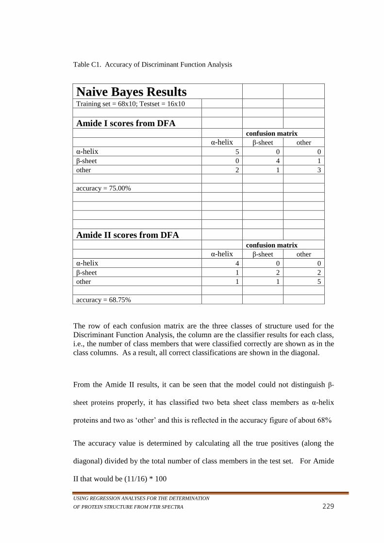
USING REGRESSION ANALYSES FOR THE DETERMINATION
OF PROTEIN STRUCTURE FROM FTIR SPECTRA 229
Table C1. Accuracy of Discriminant Function Analysis
Naive Bayes Results
Training set = 68x10; Testset = 16x10
Amide I scores from DFA
confusion matrix
α-helix β-sheet other
α-helix 5 0 0
β-sheet 0 4 1
other 2 1 3
accuracy = 75.00%
Amide II scores from DFA
confusion matrix
α-helix β-sheet other
α-helix 4 0 0
β-sheet 1 2 2
other 1 1 5
accuracy = 68.75%
The row of each confusion matrix are the three classes of structure used for the
Discriminant Function Analysis, the column are the classifier results for each class,
i.e., the number of class members that were classified correctly are shown as in the
class columns. As a result, all correct classifications are shown in the diagonal.
From the Amide II results, it can be seen that the model could not distinguish β-
sheet proteins properly, it has classified two beta sheet class members as α-helix
proteins and two as ‘other’ and this is reflected in the accuracy figure of about 68%
The accuracy value is determined by calculating all the true positives (along the
diagonal) divided by the total number of class members in the test set. For Amide
II that would be (11/16) * 100

APPENDIX
230
Appendix D
Appendix D contains a high level flow chart of the steps taken mainly for the
spectral pre-processing steps carried out in Chapter 2 and a generalized
Multivariate Analysis (MVA) flow done in Chapters 3 and 4.

USING REGRESSION ANALYSES FOR THE DETERMINATION
OF PROTEIN STRUCTURE FROM FTIR SPECTRA 231
Figure D 1. This top level flow chart represents the operations carried out in this thesis.
Level 3.0 and 4.0 can be done in the same step as part of the multivariate regression
analysis. Each step of the chart is expanded on different flow diagrams. See Figure D2
and D3 of this thesis.

APPENDIX
232
Figure D2. Step 1.0 of the flow chart highlights the steps taken for the ATR-FTIR spectra
measurements using the Bruker Tensor spectrometer with Opus 6.2 software. The process
in red is an external entity to the spectra measurement; the spectra can be saved and plotted
in any chosen plotting software.

USING REGRESSION ANALYSES FOR THE DETERMINATION
OF PROTEIN STRUCTURE FROM FTIR SPECTRA 233
Figure D3. Step 2.0 captures the pre-processing steps that were done on the ATR-FTIR
measured spectra used for this research. Each step of this flow chart was done in Matlab
R2010 and Matlab R2013a. The process in red is not necessary part of the pre-processing
steps and is expanded in Figure D4.
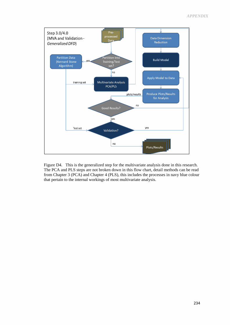
APPENDIX
234
Figure D4. This is the generalized step for the multivariate analysis done in this research.
The PCA and PLS steps are not broken down in this flow chart, detail methods can be read
from Chapter 3 (PCA) and Chapter 4 (PLS), this includes the processes in navy blue colour
that pertain to the internal workings of most multivariate analysis.