using multi-criteria analysis and gis to determine the …431811/fulltext01.pdfexamensarbete,...

Examensarbete, Kandidantnivå, 15 hp

Geomatik

Using Multi-criteria analysis and GIS to

determine the brown bear denning habitat -a case study in Sånfjället National Park, Sweden

YANJING JIA

ZIHAN LIU

2011

Bachelor’s Thesis in Geomatics

STUDY PROGRAMME FOR A DEGREE OF

BACHELOR OF SCIENCE IN GEOMATICS

Supervisor: Dr. Julia Åhlén

Examiner: Dr. Bin Jiang

Co-examiner: Mr. Peter D. Fawcett

JIA YANJING & LIU ZIHAN 2011-06-02

Abstract Human disturbance as the main factor influencing the habitat of brown bear (Ursus

arctos) has occurred frequently with the development of human society. How to

reduce and prevent the conflict between human and brown bears is considered as an

important question for brown bear conservation, management and public safety.

Sånfjället National Park has one of the densest bear populations in Sweden. Many

tourists are attracted to visit bears each year. Through this study, the most possibility

brown bear denning habitat in Sånfjället National Park was determined by using

Multi-Criteria Analysis. A customized habitat distribution map generator was

programmed within the Microsoft Visual Basic® for Applications (VBA) in ArcGIS.

Three themes were designed in the map generator, i.e., the human impact emphasis

weighted, neutral weighted themes and customized weighted theme. Customized

weighted theme was produced for user discovering denning habitat results with user-

defined weights. Comparing the final maps generated from the human impact

emphasis weighted and neutral weighted themes, human influence concentrated in the

south area of the National Park. The trails near Sveduterget should be changed to

avoid human disturbance in the bear denning period.

Keywords: Brown bear; Human influence; Denning habitat; Multi-Criteria Analysis

(MCA); Microsoft Visual Basic® for Applications (VBA); Sånfjället National Park


Table of contents

1. Introduction ................................................................................................................ 1

1.1 Aims ................................................................................................................. 1

1.2 Research Questions .......................................................................................... 2

1.3 Background ...................................................................................................... 2

2. Study Area ................................................................................................................. 4

3. Methods...................................................................................................................... 7

3.1 Data collection and data processing ................................................................. 9

3.1.1 Digital land use map ........................................................................... 10

3.1.1.1 Settlement ................................................................................ 11

3.1.1.2 Drainage and land type ............................................................ 12

3.1.1.3 Forest type ................................................................................ 13

3.1.2 Digital elevation model ....................................................................... 14

3.2 GIS analysis and customized habitat selection tool ....................................... 17

4. Results ...................................................................................................................... 20

4.1 The interface of the customized habitat distribution map generator .............. 20

4.2 The implementation results of two themes: human impact emphasis weighted

theme and neutral weighted theme ...................................................................... 22

5. Discussion and Conclusion ...................................................................................... 25

References .................................................................................................................... 26

Appendix I: Calculation of priority vector................................................................... 30

Appendix II: Computation of Maximum Eigenvalue of Normal matrix and

Consistence Ratio......................................................................................................... 30

Appendix III: Final result map generation ................................................................... 36


Acknowledgements We would like to express our appreciation to our supervisor Dr. Julia Åhlén, who

guides us patiently and gives us many advices and ideas. We are grateful to our

classmate, Tao Peng, who gives us a great help in programming. We thank our

examiner and co-examiner, Dr. Bin Jiang and Mr. Peter Fawcett, for their valuable

comments.

We would also like to thank Lantmäteriverket for providing data material. Thanks to

Scandinavian Brown Bear Research Project provide us lots of useful scientific articles.


1

1. Introduction Because of the development of the human society, bear habitat is seriously influenced.

Not only their life is threated by hunting, vehicle and train collisions and conflicts in

human benefits, but also they must avoid or tolerate human disturbance in their

denning period. In Sweden and Norway about 9% winter den abandonment happened

by brown bear (Swenson et al. 1997). Swenson et al. (1997) find that most den

abandonment was caused by human disturbance. Bears might walk maximum 30km

to find another den. Den abandonment would cause their health expense. Pregnant

females even lost their cubs.

Since time immemorial, spatial information has remained close relationship with

people’s daily life. Geographical information system (GIS) represents the process of

capturing, storing, processing, analyzing, and displaying geographical information

(Longley et al., 2005, p.28). As Burrough and McDonnell (1998) state that, in the

core area of GIS, data in a location associate with its attributes is comparable with

data in other locations. With the progress of science and technology, GIS proved to be

a powerful tool as it can process huge volume data, decrease analysis time, reduce

human resource cost and achieve vivid vision effect. GIS contributes to government,

business and environment in a mount of fields, for instance, urban management,

commercial site selection, environmental assessment, natural disaster monitoring, etc.

Among these applications, many researchers have utilized GIS based method to

search optimal habits for wildlife animals. For example, Gerrard et al. (2001) derive a

small-cell GIS raster to assess kit fox habitat.

1.1 Aims The purpose of this study is to determine the brown bear denning habitat in Sånfjället

National Park by using Multi-Criteria Analysis and VBA in ArcGIS. Bears are rarely

seen, so it is difficult to determine their habitat by field survey. GIS-based Multi-

Criteria Analysis provides an effectively method for the conservation and

management of the brown bears in Sweden. The most possible bear denning habitat

was displayed in a thematic map, and the possibility was classified into several groups.

Meanwhile, with the programming in ArcGIS, user can discover their own habitat

results with weight. This study could provide achievable suggestion for the National

Park management and effectively method for brown bear research in the whole

Scandinavia. With the help of the study, a recommendation was obtained which

intend to reduce the potential conflicts between people and brown bears, including

whether the designed tourist trail is reasonable or not considering about brown bear

encounter. It can also give the suggestion for the hikers and campers that which area

the bear frequent. For the National Park development, if they want to build more

tourist facilities, such as cabins, with this bear denning habitat selection tool, the most

possibility denning habitat area can be avoided from disturbance or destroying.

Meanwhile, with the accuracy bear habitat distribution map, researcher can study the

bear efficiently when doing the fieldwork in this area, such as the bear tracking

project.


2

1.2 Research Questions After successfully processing data, a thematic map was generated to provide solution

of following research questions:

1) What influence does human activity cause for bear denning habitat by comparing

the human influence bias result map and neutral position result map?

2) Where is the optimal habitat of brown bears?

3) What suggestion could be given for the conservation and tourism management in

Sånfjället National Park?

1.3 Background Along with increasingly extensive and intensive human activities, the rate of species

extinction is more than 100-1,000 times higher than the expected natural rate (World

Wildlife Fund, 2011). Over last century, the severe situation causes the attention of

people increasingly. The protective measures for carnivores have been taken in

increasing population, reversing trends and establish habitats (Noss et al., 1996).

Nowadays, although Swedish government protects brown bear, a few bears hunting

are allowed in some specific each year (Nature Travels, 2008). With a graceful

isolated mountain and surrounding forest, the study area, Sånfjället National Park

established in 1909 is well known as the important brown bear habitat in all of

Scandinavia (Swedish Environmental Protection Agency, 2011). Brown bear is very

secretive mammal. So it’s difficult to observe their behavior and determine their

population. One ongoing Scandinavian Brown Bear Research Project estimate the

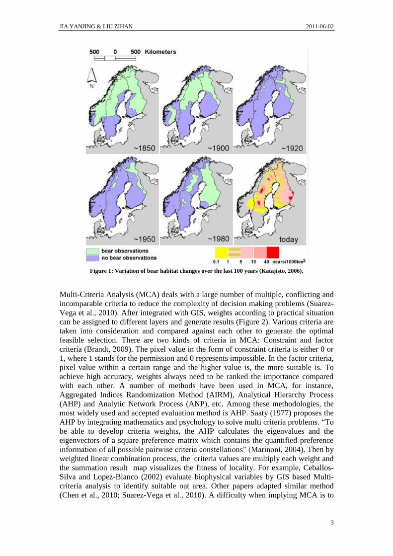
population between 1635 and 2840 individuals in the year 2004 (Figure 1). Brown

bear is a kind of omnivorous animals. In summer and autumn they eat ants, voles,

reindeers, and also berries, roots, buds of plants to store fat in their body for the

preparation of hibernation. In fact, brown bears are not true hibernators. They may

wake up occasionally or even wander outside their dens. In this period, they

metabolism is very slow and sleep through most of the winter time. Pregnant females

give birth to a cub in January or February when they are sleeping (Great Bear

Foundation, 2011). Swenson et al. (1997) represent the bears are vulnerable to

disturbance during the hibernation because of their weight loss and reproduction.

Elfström et al. (2008) prove that the habitat preference slightly changes with the age

or sex. Bears prefer open canopy forest than closed canopy forest, and like the habitat

with moist soil. Water, deciduous forest, peat, exposed bedrock and gravel pits are

improper for the inhabitance of bears. Additionally, compared with available bears,

the number of denned bears was found more in areas with lower altitudes, easterly

aspects and steeper slopes. As human disturbance is the main factor influence the

brown bear density, bears except for the young individuals mainly distributed up to

10km from human settlement (Kindberg, 2010). Linnell et al. (2000) indicate that

more than 1km is the distance which bear could tolerant human disturbances,

including roads and industrial activity.


3

Figure 1: Variation of bear habitat changes over the last 100 years (Katajisto, 2006).

Multi-Criteria Analysis (MCA) deals with a large number of multiple, conflicting and

incomparable criteria to reduce the complexity of decision making problems (Suarez-

Vega et al., 2010). After integrated with GIS, weights according to practical situation

can be assigned to different layers and generate results (Figure 2). Various criteria are

taken into consideration and compared against each other to generate the optimal

feasible selection. There are two kinds of criteria in MCA: Constraint and factor

criteria (Brandt, 2009). The pixel value in the form of constraint criteria is either 0 or

1, where 1 stands for the permission and 0 represents impossible. In the factor criteria,

pixel value within a certain range and the higher value is, the more suitable is. To

achieve high accuracy, weights always need to be ranked the importance compared

with each other. A number of methods have been used in MCA, for instance,

Aggregated Indices Randomization Method (AIRM), Analytical Hierarchy Process

(AHP) and Analytic Network Process (ANP), etc. Among these methodologies, the

most widely used and accepted evaluation method is AHP. Saaty (1977) proposes the

AHP by integrating mathematics and psychology to solve multi criteria problems. “To

be able to develop criteria weights, the AHP calculates the eigenvalues and the

eigenvectors of a square preference matrix which contains the quantified preference

information of all possible pairwise criteria constellations” (Marinoni, 2004). Then by

weighted linear combination process, the criteria values are multiply each weight and

the summation result map visualizes the fitness of locality. For example, Ceballos-

Silva and Lopez-Blanco (2002) evaluate biophysical variables by GIS based Multi-

criteria analysis to identify suitable oat area. Other papers adapted similar method

(Chen et al., 2010; Suarez-Vega et al., 2010). A difficulty when implying MCA is to


4

determine credible weights. The stakeholders compare importance of each criterion

leading the existence of large subjectivity.

Figure 2: An example of GIS based Multi-Criteria Decision Analysis.

With the rapid development of computer technology, the computers have equipped

with modern accessories and maintain better performance. A great number of

software developed, and one of the most successful is the ArcGIS developed by ESRI

Company. It helps user with asset or data management, planning and analysis,

business operations and situational awareness (ESRI, 2011). The commercial software

designate to multitude, so just basic and general functions are owned by it. While

ArcGIS enables user to plan, design and implement their own customized tools to

solve related questions. By using ArcObjects and Visual Basic for Application (VBA)

into ArcGIS, weights in MCA can be specified by users and final result map can be

visualized by clicking a customized button in ArcMap.

2. Study Area The study area, Sånfjället National Park (62°17′N 13°32′E) was conducted in the

country of Härjedalen in the middle of Sweden (Figure 3). It was established in 1909

and takes about 104 km2 after extended in 1989.


5

Figure 3: The study area of brown bear habitat in Sånfjället National Park (Naturvårdsverket, 2011).

Härjedalen contains a wealth of nature resources and tourism resources. About 9000

years ago, the first population appeared living on fishing and hunting. Since 17th

century, the Lapps and their reindeer have played an important role in the history of

Härjedalen. Nowadays, there are only 11000 inhabitants living in this 12000 square

kilometers county. Härjedalen, this wildness area is a paradise for wild animals and

plants. Bears, moose, wolfs, lynx have lived in their nature habitat for centuries. More

than 400 species of flowers grow on the mountain, including very rare orchids. Not

only the county symbol of Härjedalen is a bear, but there is also a 13 meters high

figure of the world’s largest wooden bear. That is because the Sånfjället National Park

in Härjedalen has one of the densest bear populations in the country (Härjedalen

Kommun, 2009). In the thematic map of bear distribution data in 1998-2003 surveyed

by Scandinavian Brown Bear Research Project, Sånfjället is in the one of the largest

value area of observations per hour average (Figure 4).

Sånfjället is known as one of the first National Parks both in Sweden and in the whole

Europe. For the purpose of the finest natural beauty protection, Sånfjället National

Park was found in 1909. Covered with lichen layer, the isolated mountain reaches

1278 meters high. At first, the National Park just contains the alpine area. In 1989, the

surrounding forest was also included in the protection (The County Administrative

Board of Jämtland, 2009).


6

Figure 4: Bear observations average 1998-2003 produced by Scandinavian Brown Bear Research Project

(Scandinavian Brown Bear Research Project, 2004).

Bears habitat depends partly on the landscapes type or vegetation zone. Basically, the

vegetation zone of Sweden is cataloged into six classes: alpine zone, northern boreal

zone, middle boreal zone, Southern boreal zone, boreo-nemoral zone and nemoral

zone (Figure 5). Alpine zone and northern boreal zone is concentrated in the northern

part of border with Norway. Sånfjället National Park is just in these two vegetation

zone. The landscapes are bare mountain and coniferous forests respectively (National

Atlas of Sweden, 2003) and which is exactly the bear prefer. That is one of the

reasons why Sånfjället National Park distributes more bears than other areas. Because

frost weathering process and the rain lashed on the Sånfjället’s slopes, just the coarse,

nutrient-poor soils left. On the bare mountain, only various types of lichens, trailing

azalea and diapensia can survive in the extreme weather condition and scrawny soil.

The forests in the Sånfjället National Park consist of three main parts: Spruce in the

Ryå ravine, mixed forest along Valmen and Styggtjärn and birch forests around

Nyvallen. All creature on the earth need water to stay alive. The river in Sånfjället

National Park can be treated as meltwater. In fact, glacial rivers shaped the land in the

most recent Ice Age. As the traces, these spillways or canyons still can be found

between the peaks (The County Administrative Board of Jämtland, 2009). As the

Meteorological statistic data from 1961 to 1990 reported by Swedish Meteorological

and Hydrological Institute (2011), the mean annual temperature is 0℃, ranging from -

15℃ in December to 17℃ in July. The average annual precipitation is 800mm. Each

year, about 175-200 days are covered with snow and the average maximum snow

depth is 90-110cm. With a long period deep snow covered, this place is also a winter

resort for various snow activities. The official park map (figure 3) shows that several

tourist trails radiate from the center of the National Park. One of them is specialized


7

winter trail. But, for the environmental protection, snowmobiles are forbidden to

access the entire park area. As The County Administrative Board of Jämtland (2009)

indicates, the service facilities in Sånfjället National Park include parking areas,

information boards, picnic places, shelters, earth toilets and cabins. These facilities

are found at the three main visitor centers. They are Nyvallen, Nysätern and Valmen

which are on the edge of the National Park (see Figure 3). In addition, an earth toilet,

a picnic place and an emergency shelter are placed in the valley south-west of mount

Högfjället. Two simple built wind shelters are also located in a valley between two

mountain tops and a wetland area near Stor-Ryvålen at the foot of the mountain

respectively. These facilities are also shown in Figure 3. The National Park also

provides fully equipped wooden cabins for visitors hiring at Nyvallen, Nysätern and

Dalsvallen on the edge of the National Park.

Figure 5: Vegetation zone of Sweden (National Atlas of Sweden, 2003)

3. Methods The study can be considered in two phases. Data collection and processing was the

first phase, from the raw data to well-prepared data for the further Multi-Criteria

Analysis. The second phase included GIS analysis and customized habitat distribution

map generators programming by using ArcObjects and Visual Basic for Application

(VBA) into ArcGIS. The flowchart of the process is shown in Figure 6. In this study,


8

ERDAS IMAGINE 9.3 and ArcMap 9.3 computer software were used for data

processing, GIS analysis and programming. ArcScene 9.3 was contributed to visualize

final result map in three-dimensional.

Figure 6: The flowchart.

The original data

The criteria layers

The weighted themes

The final maps

Constraint Map

Factor Map

Required criteria

Optional criteria


9

3.1 Data collection and data processing Data collection of the thesis was mainly based on Digitala Kartbiblioteket i

SWEREF99 from Lantmäteriverket. This Digital Map Library provides researcher

various map data covering the entire Sweden, such as Orthophoto and digital

elevation model. Depending on the brown bear behavior and living requirement,

several criteria should be concerned, such as slope, elevation, drainage, settlement,

road, forest density and so on. These layers were obtained from digital elevation

model and digital land use map (figure 7). According to their attitude and the impact

on bear denning habitat, these criteria were made into constraint and factor maps

(Table 1). To make sure these two types of map data were covering the same area, the

coordinates of two ending points (assume they were point a, b) on the rectangle

diagonal line should be exactly the same. In SWEREF99 reference system, point a

was (6915311, 432797) and point b was (6896186, 416987).

Figure 7: The original digital land use map image (left) and digital elevation model image (right) covering

the study area.


10

Table 1: Denning habitat criteria and their corresponding constraint and factor zones

Denning

habitat

criteria

Data

Source

Constraint zones Factor zones

Settlement Land use

map

<1km=0 Suitability was

proportional to

distance

Drainage water=0 Suitability was

proportional to

distance

Land type Wetland=50,

Exposed rock and

sparse land=50

Forest type coniferous

forest=255,

young forest and

mixed forest=150,

Selectively logged

forest=100,

Bushes and

deciduous forest=50

Slope

Digital

elevation

model

(DEM)

>10.6°=0

<0.6°=0

Suitability was

proportional to slope

Aspect Southwestern(202.5°~247.5°)=0,

western(247.5°~292.5°)=0,

northwestern(292.5°~337.5°)=0,

northern(0°~22.5°&337.5°~360°)=0,

northeastern(22.5°~67.5°)=0

Eastern(67.5°-

112.5°)=255,

Southeastern(112.5°-

157.5°) and

southern(157.5°-

202.5°)=150

elevation >620.9m=0

<378.5m=0

Suitability was

inversely proportion

to elevation

3.1.1 Digital land use map

The digital land use map on the digital map library had already been classified into

dozens of types, from settlement type to forest density. So, there was no need to

collect data from original satellite image by using supervised or unsupervised

classification method. The criteria for this study were selected separately by using

recoding in Erdas 9.3 according to the legend. Finally, settlement, drainage, land type

and vegetation type were collected as the criteria layer and totally 12 sub-criteria were

divided in several layers (Figure 8).


11

Figure 8: The recoded land use map

3.1.1.1 Settlement

The brown bear is a very bashful animal. They prefer the place where the human

influence is lowest. Especially in winter, Petram et al. (2004) claim that brown bears

are very sensitive during the hibernation period. They are very aggressive if they feel

human disturbances during this period. Since there is no motorway in the National

Park and the snowmobiles is also prohibited, in this study human settlement was

treated as human influence, an important habitat factor. In Slovenia, Petram et al.

(2004) have showed that brown bears prefer to choose caves in the steep ravines and

large karst dolines for winter dens where human cannot easily access. They compared

the caves in four different landscape type, the karst plateau, big dolines, canyons and

river valley area. Big doline had more probability for cave choice by brown bears than

karst plateau. After doing statistic of the distance between the caves of all landscape

types and villages, they obtained that the dens of brown bears was at least 540m away

from village. Due to the human activities, such as forestry survey activity, roe deer

hunter, ice fishing and so on, den abandonment may happen when bears feel

disturbance. Sweson et al. (1997) describe that it would causes the result of fitness

cost and danger of abortion for pregnant females. When bears abandoned a den, they

would dig a new den, or just lay on the ground with branches bed in a few hundred

meters away, or walking even further. For the bear conservation from minimizing den

abandonment, and the human safety reason, Sweson et al. (1997) suggest that human

activity should keep distance from the active bear dens at least 100m, or maybe up to

1 km. Because of their data collection limitation, they didn’t provide an accuracy

figure of the distance. Linnell et al. (2000) indicate that more than 1km is the distance

which bear could tolerant human disturbances, including roads and industrial activity.

In this study, human settlement contained rural settlement, camping and holiday

house, and arable land and farm (Figure 9). The suitability value was 0 within 1 km.

In the area larger than 1 km, suitability was proportional to distance.


12

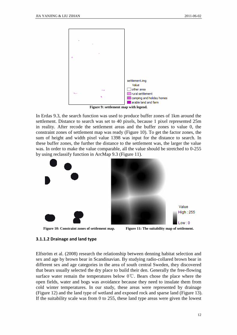
Figure 9: settlement map with legend.

In Erdas 9.3, the search function was used to produce buffer zones of 1km around the

settlement. Distance to search was set to 40 pixels, because 1 pixel represented 25m

in reality. After recode the settlement areas and the buffer zones to value 0, the

constraint zones of settlement map was ready (Figure 10). To get the factor zones, the

sum of height and width pixel value 1398 was input for the distance to search. In

these buffer zones, the further the distance to the settlement was, the larger the value

was. In order to make the value comparable, all the value should be stretched to 0-255

by using reclassify function in ArcMap 9.3 (Figure 11).

Figure 10: Constraint zones of settlement map. Figure 11: The suitability map of settlement.

3.1.1.2 Drainage and land type

Elfström et al. (2008) research the relationship between denning habitat selection and

sex and age by brown bear in Scandinavian. By studying radio-collared brown bear in

different sex and age categories in the area of south central Sweden, they discovered

that bears usually selected the dry place to build their den. Generally the free-flowing

surface water remain the temperatures below 0℃. Bears chose the place where the

open fields, water and bogs was avoidance because they need to insulate them from

cold winter temperatures. In our study, these areas were represented by drainage

(Figure 12) and the land type of wetland and exposed rock and sparse land (Figure 13).

If the suitability scale was from 0 to 255, these land type areas were given the lowest


13

values of 50, according to the suitability ranking. And suitability increase with the

distance from the drainage.

First of all, the drainage area was recoded to the value 0 in Erdas 9.3. Factor zones

were also obtained from search function in Erdas while the distance to search was set

to 1398, as the sum of height and width pixel value. The suitability value was

proportional to the distance from drainage. At first, the pixel values were ranging

from 0 to 527. After reclassify processing in ArcMap 9.3, these pixel values were

stretched from 0 to 255 (Figure 14). Land type map didn’t produce the buffer zones.

The value of 50 was given directly through the reclassify function in ArcMap to the

land type of wetland and exposed rock and sparse land instead (Figure 15).

Figure 12: Drainage map with legend Figure 13: Land type map with legend

Figure 14: The suitability map of drainage. Figure 15: The suitability map of land type.

3.1.1.3 Forest type

According to the dominant species, the forest type in Sånfjället National Park was

divided into several groups. These were deciduous forest, coniferous forest, mixed

forest, bushes, selectively logged forest and young forest (Figure 16). After analyzing

by a ranking matrix of brown bear winter dens, Elfström et al. (2008) show that

denning bears don’t like alpine mountain-birch forest and deciduous forest. Instead,

they prefer coniferous forest, young forest and selectively logged forest. Ciarniello et

al. (2005) also find that there were “no dens in black spruce, shrubs, meadows,

swamps, rock-bare ground, or anthropogenic landscapes.” Therefore, Bushes was the

lowest suitable forest type of bear habitat. As Petram et al. (2003) describe, bear


14

habitat consisted mixed, uneven aged forests with “varying amounts of spruce (Picea

abies), sycamore (Acer pseudoplatanus) and elm (Ulmus sp.)”. So, mixed forest type

would be considered as one of the suitable forest types for dens by brown bear. After

estimating the suitability of each forest type, these were reclassified as several values

in a factor map by using ArcMap 9.3. The most suitable ranking type coniferous

forest was given the highest values of 255. Then young forest and mixed forest as the

moderate ranked at 150. Selectively logged forest also showed little use had the value

of 100. Bushes and deciduous forest represented by the lowest value 50 (Figure 17).

Figure 16: Forest type map with legend.

Figure 17: The suitability map of forest type.

3.1.2 Digital elevation model

From the digital elevation model (DEM), elevation, aspect and slope could be

obtained. DEM as a raster format contained elevation value in each pixel. In ArcMap

9.3, with the help of spatial analysis tool, a layer of slope (Figure 18) and aspect

(Figure 19) can be generated from digital elevation model. The elevation ranging

from 422.5m to 1274.8m had the largest value in the center of the park with the flat

area surrounding (Figure 20). The value of slope in Sånfjället National Park was

ranging from 0° to 38.9066°.In the previous study, critical value for brown bear

denning habitat suitability in Scandinavian has been reported by Elfström et al. (2008).

They list the mean values and corresponding standard derivation of elevation and

slope with different categories of age and gender respectively. In our study, only the


15

values for all bear categories were used. Those were elevation 378.5m~620.9m and

slope 0.6°~10.6°. As Elfström et al. (2008) report “lower altitude, easterly aspect and

steeper slope” were the conditions of bear denning habitat selection. Ciarniello et al.

(2005) state bear prefer steep slopes to avoid human access. Li et al. (1994) report the

most dens were found on the eastern, southeastern and southern aspect. The reason

why is that solar energy could provide heat for bear to against the bitter cold. The

other reason explained by Schoen et al. (1987) is that easterly aspect would

accumulate greatest snowpack which resulted satisfactory den insulating effect for

Scandinavian bear dens.

Figure 18: The slope map with legend

Figure 19: The aspect map with legend


16

Figure 20: The elevation map with legend.

By using raster calculator in ArcMap 9.3, the areas with the elevation lower than

620.9m were selected. After reclassified, all elevation values were stretched from 0 to

255. Since the suitability value increased as the elevation decreased, raster calculator

was used to subtract the stretched image from 255. Now, higher value represented

more suitable habitat areas in lower elevation (Figure 21). Meanwhile, the slope value

from 0.6° to 10.6° was selected and stretched in ArcMap (Figure 22). As for aspect,

all the other aspects except eastern, southern and southeastern were reclassified into 0.

Eastern had the highest value of 255. Southeastern and southern were given the value

of 150 (Figure 23).

Figure 21: The suitability map of elevation Figure 22: The suitability map of slope.


17

Figure 23: The suitability map of aspect

3.2 GIS analysis and customized habitat selection tool The accomplishment of layer decision and raster dataset generation processes leaded

to the initial phase of VBA programming in ArcMap 9.3. A customized toolbar

designed to facilitate user to select relevant layers was developed in this section.

The core of the bear habitat selection tool was the determination of criteria’s weight.

Analytical Hierarchy Process (AHP) was utilized in the system to decide the multi

criteria’s weight. By comparing the relative relevance of every two criteria, values

from 1 to 9 were assigned according the importance of each criterion (Table 2), where

1 representing few variation, 9 standing for the extremely importance difference

between two criteria and the other integers between 1 to 9 shows gradual change of

relevance. Table 2: Judgment of relevance value in AHP (Saaty and Vargas, 1991, p.251).

Judgment of relevance Value

Equal Importance

Weak Importance of one over another

Essential or Strong Importance

Demonstrated Importance

Absolute Importance

Intermediate value between the two adjacent judgments

If cell a(i,j) has one of the previous value, then cell a(j,i) was assigned

the reciprocal value. (a(i,j)*a(j,i)=1)

1

3

5

7

9

2,4,6,8

Reciprocals

The symmetrical entries’ product equaled to 1, so the user only need to choose the

value of pairwise comparison value below the diagonal line. Mortenson (no date)

provides several groups of pairwise comparison matrix values for the project of

grizzly bear habitat assessing in GIS. Since the criteria and purpose were very similar

with our research. The weights of human impact emphasis weighted theme (Table 3)

and neutral weighted theme (Table 4) were assigned by referencing Mortenson’s

project.


18

Table 3:Pairwise comparison matrix in human impact emphasis weighted theme

CRITERIA Distance

to

settlement

Distance

to

drainage

Elevation Slope Aspect Land

type

Forest

type

Distance to

settlement

1 5 3 3 3 2 2

Distance to

drainage

1/5 1 1/3 1/2 1/2 1/4 1/4

Elevation 1/3 3 1 2 2 1/2 1/2

Slope 1/3 2 1/2 1 1 1/2 1/2

Aspect 1/3 2 1/2 1 1 1/2 1

Land type 1/2 4 2 2 2 1 1

Forest type 1/2 4 2 2 1 1 1

Table 4: Pairwise comparison matrix in neutrality weighted theme

CRITERIA Distance

to

settlement

Distance

to

drainage

Elevation Slope Aspect Land

type

Forest

type

Distance to

settlement

1 2 1/2 1 1 1/3 1/3

Distance to

drainage

1/2 1 1/3 1/2 1/2 1/3 1/3

Elevation 2 3 1 2 2 1/2 1/2

Slope 1 2 1/2 1 1 1/2 1/2

Aspect 1 2 1/2 1 1 1 1/2

Land type 3 3 2 2 1 1 1/2

Forest type 3 3 2 2 2 2 1

Supposed the generated pairwise comparison judgment matrix A has i row and j

column and entries aij, then the formula of priority vector calculation consists of three

steps:

1. Normalize every column of A: ∑ (1)

2. Sum entities of in one row: ∑ (2)

3. Normalize : ∑ (3)

The is the priority vector of judgment matrix A with property∑ , and i is the

i-th selected criterion. To ensure the priority vector credible and reduce subjective

human judgment error, consistency check is essential (Madhuri, et al., 2010). As Lin

and Yang (1996) state that An*n consistent matrix A’s maximum eigenvalue should

equal to n. While due to the practical calculation deviation, A cannot be the consistent

matrix. So, Saaty developed a method utilizing Consistence Index (CI) and Random

Consistency Index (RI) to measure the degree of consistency variation. The

consistence index (CI) is computed by the following formula:

(4)


19

The Random Consistency Index (RI) was the average of 500 reciprocal matrices (with

value 1,2…9 and 1/2,1/3…1/9) generated randomly (Kardi, 2006). The value of RI

with order from 1 to 10 was shown in the Table 4. Table 4: Random Consistency Index value from n=1 to 10 (Kardi, 2006).

n 1 2 3 4 5 6 7 8 9 10

RI 0 0 0.58 0.9 1.12 1.24 1.32 1.41 1.45 1.49

The Consistence Ratio with optimal value 0 could be accepted less than 0.1.

Algorithm for CR is:

(5)

Finally, the remaining question is how to calculate the maximum eigenvalue. First

change the pairwise comparison judgment matrix to Hessenberg matrix by the use of

stabilized elementary matrix. To transfer a normal matrix to Hessenberg form, n-2

steps taken for the matrix Ai*j. Matin and Wilkinson (1968) use formula to expound

the r-th step in real matrix transformation:

(1) Determine the maximum non zero entity: | ( )|( ) . The

maximum element is denoted by | ( )

( )| If the maximum entity value equals to

zero, skip this r-th step. (2) Switch rows (r+1)’ with (r+1) and columns (r+1)’ with (r+1).

(3) For each i changes from r+2 to n, ( )

( )

, subtract × row r+1

from row I and add × column i to column r+1.

( ) ( ) , (6)

Where ( ) is an elementary permutation matrix and is an elementary

matrix with

( ) ( ) and ( ) (7)

Then, Solve all the eigenvalue of Hessenberg matrix with QR method proposed by

Franeis in 1960. The formula of Hessenberg matrix (Hi,j) calculated by the following

formula:

(8)

( ) (9)

where is the eigenvector of H, is eigenvalue of H and I is the Identity matrix with

the same stage of H. The eigenvalues may be real or imaginary, and complex numbers

cannot compare value. Therefore, the imaginary eigenvalues were abandoned and the

maximum real eigenvalue was we desired. Eigenvalues of matrix Ai,j are equivalent to

the Hessenerg Hi,j . The consistence ratio was identified by Formula (5). Warning

message was shown when consistence ratio larger than 0.1 and a recalculation was

recommended. Value less than 0.1 dignified priority vector credible and was

incorporated into the final result map analysis.

Final result map was computed by a linear combination of relevant criteria (Nyoman

et al., 2008). The variable wi represents priority vector, ai,j is the stretched factor or

constraint raster dataset.

∑ (10)

Until now, the final result map was generated, while it would be more informatics

through a series of following interpretation and enhancement.


20

4. Results There were three themes (human impact emphasis, neutral weighted and customized

criteria) with distinct intentions implemented in the customized habitat distribution

map generator. Human impact emphasis analysis stressed on the human factor

influence on the bear distribution, in this case, the human settlement criterion

weighted high than others. Dissimilar to the first theme, neutral weight

comprehensively considered the entire seven layers. The last theme enabled user to

select criteria and weight based on their own opinions. The previous two themes were

pre-assigned pairwise comparison value and user assigned the matrix value. By

selecting pairwise comparison value from the list boxes, each criteria weight and

consistence ration was calculated. After obtaining rational weights (consistence ration

< 0.1), the number of classes and legend of final result map were modified to get a

higher vision effect. Buffers could be created depending on the user’s decision to

visualize the bear habitat’s impaction on the tourist and human activity.

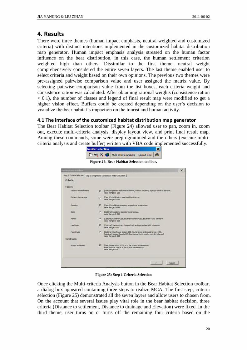
4.1 The interface of the customized habitat distribution map generator The Bear Habitat Selection toolbar (Figure 24) allowed user to pan, zoom in, zoom

out, execute multi-criteria analysis, display layout view, and print final result map.

Among these commands, some were preprogrammed and the others (execute multi-

criteria analysis and create buffer) written with VBA code implemented successfully.

Figure 24: Bear Habitat Selection toolbar.

Figure 25: Step 1 Criteria Selection

Once clicking the Multi-criteria Analysis button in the Bear Habitat Selection toolbar,

a dialog box appeared containing three steps to realize MCA. The first step, criteria

selection (Figure 25) demonstrated all the seven layers and allow users to chosen from.

On the account that several issues play vital role in the bear habitat decision, three

criteria (Distance to settlement, Distance to drainage and Elevation) were fixed. In the

third theme, user turns on or turns off the remaining four criteria based on the


21

suggestions in the right part of interface depending on their own view of the relevance.

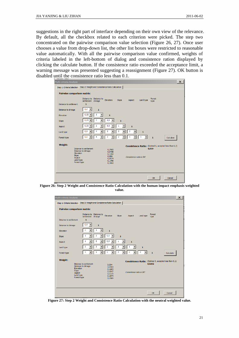
By default, all the checkbox related to each criterion were picked. The step two

concentrated on the pairwise comparison value selection (Figure 26, 27). Once user

chooses a value from drop-down list, the other list boxes were restricted to reasonable

value automatically. With all the pairwise comparison value confirmed, weights of

criteria labeled in the left-bottom of dialog and consistence ration displayed by

clicking the calculate button. If the consistence ratio exceeded the acceptance limit, a

warning message was presented suggesting a reassignment (Figure 27). OK button is

disabled until the consistence ratio less than 0.1.

Figure 26: Step 2 Weight and Consistence Ratio Calculation with the human impact emphasis weighted

value.

Figure 27: Step 2 Weight and Consistence Ratio Calculation with the neutral weighted value.


22

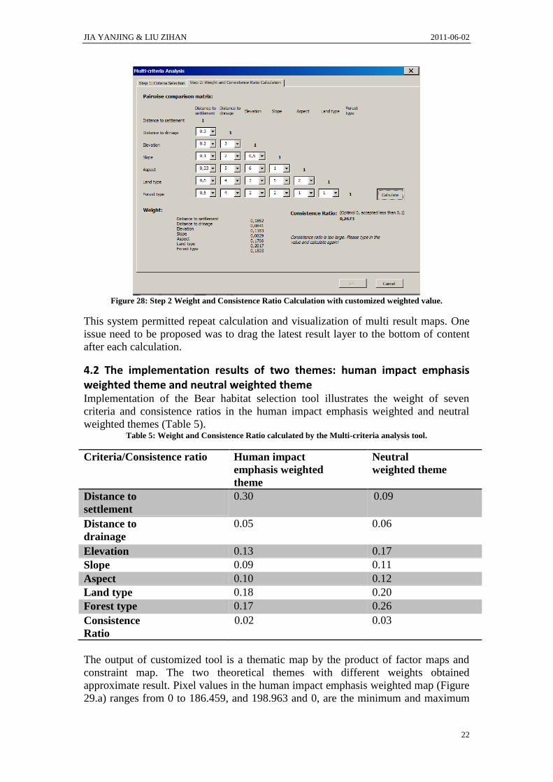
Figure 28: Step 2 Weight and Consistence Ratio Calculation with customized weighted value.

This system permitted repeat calculation and visualization of multi result maps. One

issue need to be proposed was to drag the latest result layer to the bottom of content

after each calculation.

4.2 The implementation results of two themes: human impact emphasis weighted theme and neutral weighted theme Implementation of the Bear habitat selection tool illustrates the weight of seven

criteria and consistence ratios in the human impact emphasis weighted and neutral

weighted themes (Table 5). Table 5: Weight and Consistence Ratio calculated by the Multi-criteria analysis tool.

Criteria/Consistence ratio Human impact

emphasis weighted

theme

Neutral

weighted theme

Distance to

settlement

0.30 0.09

Distance to

drainage

0.05 0.06

Elevation 0.13 0.17

Slope 0.09 0.11

Aspect 0.10 0.12

Land type 0.18 0.20

Forest type 0.17 0.26

Consistence

Ratio

0.02 0.03

The output of customized tool is a thematic map by the product of factor maps and

constraint map. The two theoretical themes with different weights obtained

approximate result. Pixel values in the human impact emphasis weighted map (Figure

29.a) ranges from 0 to 186.459, and 198.963 and 0, are the minimum and maximum


23

value of neutral weighted theme map (Figure 29.b). To enhance map readability and

reduce data fusion, maps are classified into nine layers respectively with marked red

representing the optimal habitat location (Figure 29.c, 29.d). About 7.862% (8.1 km2)

and 6.052% (6.3 km2) area mainly distributed in the eastern and a few in the western

of part of high elevation area were selected in Sånfjället National Park. 3D views

utilizing DEM as base height were interpreted in ArcScene 9.3 to increase

intuitionistic (Figure 30.e and 30.f). Z unit conversion was set to 4 to amplify the

elevation difference.

(a) Human impact emphasis weighted theme. (b) Neutral weighted theme based result map.

(c) Map classification of Human impact emphasis (d) Map classification of Neutral

weighted theme weighted theme

Figure 29: Final result map of bear distribution (Part 1).


24

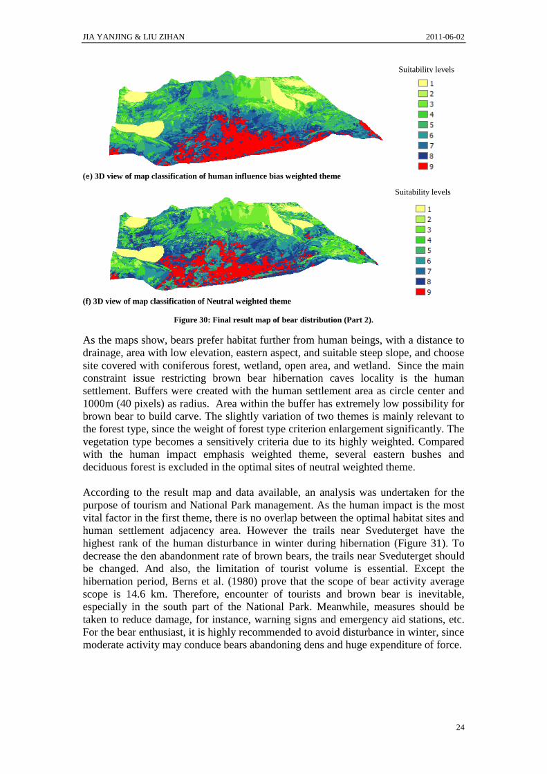
(e) 3D view of map classification of human influence bias weighted theme

(f) 3D view of map classification of Neutral weighted theme

Figure 30: Final result map of bear distribution (Part 2).

As the maps show, bears prefer habitat further from human beings, with a distance to

drainage, area with low elevation, eastern aspect, and suitable steep slope, and choose

site covered with coniferous forest, wetland, open area, and wetland. Since the main

constraint issue restricting brown bear hibernation caves locality is the human

settlement. Buffers were created with the human settlement area as circle center and

1000m (40 pixels) as radius. Area within the buffer has extremely low possibility for

brown bear to build carve. The slightly variation of two themes is mainly relevant to

the forest type, since the weight of forest type criterion enlargement significantly. The

vegetation type becomes a sensitively criteria due to its highly weighted. Compared

with the human impact emphasis weighted theme, several eastern bushes and

deciduous forest is excluded in the optimal sites of neutral weighted theme.

According to the result map and data available, an analysis was undertaken for the

purpose of tourism and National Park management. As the human impact is the most

vital factor in the first theme, there is no overlap between the optimal habitat sites and

human settlement adjacency area. However the trails near Sveduterget have the

highest rank of the human disturbance in winter during hibernation (Figure 31). To

decrease the den abandonment rate of brown bears, the trails near Sveduterget should

be changed. And also, the limitation of tourist volume is essential. Except the

hibernation period, Berns et al. (1980) prove that the scope of bear activity average

scope is 14.6 km. Therefore, encounter of tourists and brown bear is inevitable,

especially in the south part of the National Park. Meanwhile, measures should be

taken to reduce damage, for instance, warning signs and emergency aid stations, etc.

For the bear enthusiast, it is highly recommended to avoid disturbance in winter, since

moderate activity may conduce bears abandoning dens and huge expenditure of force.

Suitability levels

Suitability levels


25

Figure 31: Trials and Facilities in the Sånfjället National Park (Thörnelöf, 2011).

5. Discussion and Conclusion This study developed a customized AHP tool with VBA in ArcMap. Integrated with

the user’s opinion, final result map clearly reflected the optimal site distribution of

bear dens in hibernation period. Suggestions were given to improve the Sånfjället

national park facilities and visitors. However, for the future perspective, some factors

can be improved. In the designed habitat generator programming, the application runs

quite slowly. It takes a long time for layer loading in criteria selection step. After the

weight is input in the second step, consistence ration is calculated to determine

whether the weight set is acceptable or not. This process also takes some time for

calculating. Maybe it is because of the large layer data size and complex matrix

calculation.

Although this study further emphasizes the bear denning habitat, in fact, brown bears

are not true hibernators. They may wake up occasionally or even wander outside their

dens. The bear home range is the activity area around bear den habitat. According to

the different type of bears such as males, single females and maternal females, the

home range size can be various. In non-denning season, they spent the most of their

time foraging and wandering within the relatively small area. As Berns et al. (1980)

report that males have the average home range size 24.4, while the average home

range size of single females and maternal females is 14.3 and 10.6 respectively.

Berland et al. (2008) indicate that a lower home range size value for adult female,

about 3~6.4km. In denning season, brown bears also wander outside occasionally but

near their den site. So the human-bear encounters as a potential danger for hikers and

skier should be avoided near the bear den site.


26

The final results are basically the same as anticipation. Although GIS and Multi-

Criteria Analysis is an efficient method for denning habitat determination, but if we

can combine the field survey data, the results will be more accuracy. So far, the

biogeographic history and field survey data for brown bears in the study area is still

deficient. We hope the brown bear conservation issue can be paid more and more

attention in the further.

References Berns, V.D., Atwell, G.C. And Boone, D.L. (1980) Brown bear movements and

habitat use at karluk lake, Kodiak Island. Bears: Their Biology and Management,

Volume 4, pp. 293-296

Berland, A., Nelson, T., Stenhouse, G., Graham, K. and Cranston, J. (2008) The

impact of landscape disturbance on grizzly bear habitat use in the Foothills Model

Forest, Alberta, Canada. Forest Ecology and Management, Volume 256, pp.1875–

1883

Brandt, A. (2009) Lecture of course Remote Sensing and GIS Analysis in Land

Management. University of Gävle, Sweden

Burrow, P.A. and McDonnell, R.A. (1998) Principle of Geographical Information

System, Oxford University Press, pp.327

Ceballos-Silva, A. and Lopez-Blanco, J. (2002) Evaluating biophysical variables to

identify suitable areas for oat in Central Mexico: a multi-criteria and GIS approach,

Agriculture, Ecosystems and Environment ,volume 95, pp. 371-377

Chen, Y., Yu, J. and Khan, S. (2010) Spatial sensitivity analysis of multi-criteria

weights in GIS-based land suitability evaluation. Environmental Modeling &

Software ,volume 25, pp. 1582-1591

Ciarniello, L.M., Boyce, M.S., Heard, D.C. and Seip, D.R. (2005) Denning behavior

and den site selection of grizzly bears along the Parsnip River, British Columbia,

Canada. Ursus, volume 16(1), pp.47-58

Elfström, M., Swenson, J. E., and Ball J.P.(2008) Selection of denning habitats by

Scandinavian brown bears. Wildlife Biology, volume 14, pp.176-187

ESRI. (2011) ArcGIS- A Complete Integrated System. Available at:

http://www.esri.com/software/arcgis/index.html (Accessed date: 4th

May, 2011)

Gerrard, R., Stine, P., Church, R. and Gllpin, M. (2001) Habitat evaluation using GIS:

A case study applied to the San Joaquin Kit Fox. Landscape and Urban Planning,

volume 52, pp.239-255

Great Bear Foundation. (2011) Brown Bear (ursus arctos). Available at:

http://greatbear.org/bear-species/ (Accessed date: 26th

May, 2011)


27

Härjedalen Kommun. (2009) Magnificent Härjedalen. Available at:

http://www.harjedalen.se/turism/english.4.1c2eb66911fa755d3678000221.html

(Accessed date: 19th

May, 2011)

Kardi, T. (2006) Analytic Hierarchy Process (AHP) tutorial. Available at:

http://people.revoledu.com/kardi/tutorial/ahp/ (Accessed date: 29th

May, 2011)

Katajisto, J.(2006) Habitat use and population dynamics of brown bears (Ursus

arctos) in Scandinavia. PhD thesis. University of Helsinki, Helsinki, Finland.

Kindberg, J. (2010) Monitoring and Management of the Swedish Brown Bear (Ursus

arctos) Population. Doctoral thesis. Dept. of Wildlife, Fish, and Environmental

Studies, SLU.

Li, X., Yiqing, M., Zhongxin, G. & Fuyuan, L. (1994) Characteristics of dens and

selection of denning habitat for bears in the south Xiaoxinganling Mountains, China.

International Conference on Bear Research and Management, volume 9, pp. 357-362.

Lin, Z.C. and Yang, C.B. (1996) Evaluation of machine selection by the AHP method.

Materials Processing Technology, volume 57, pp. 253-258

Linnell, J.D.C, Swenson, J.E., Andersen, R., and Barnes, B. (2000) How vulnerable

are denning bears to disturbance? Wildlife Society Bulletin, Volume 28, pp.400-413

Longley, P.A., Goodchild, M.F., Maguire, D.J., and Rhind, D.W. (2005) Geographic

Information Systems and Sciences. Chichester: Wiley. 2nd edition

Madhuri, C.B., Padmaja, M., Rao, T.S., and Chandulal, J.A. (2010) Evaluating web

site based on Grey Clustering Theory combined with AHP. International Journal of

Engineering and Technology, volume 2(2), pp.71-76

Marinoni, O. (2004) Implementation of the analytical hierarchy process with VBA in

ArcGIS. Computers & Geosciences, volume 30, pp. 637-646

Martin, R.S., and Wilkinson, J.H. (1968) Similarity Reduction of a General Matrix to

Hessenberg form. Numer. Math. volume 12, pp.349-368

Mortenson, C. (No date) Effectiveness of GIS in assessing grizzly bear habitat in the

Central Coast of British Columbia. Available at:

http://www.sfu.ca/geog355fall02/cmortenb/project.html (Accessed date: 2nd

June,

2011)

National Atlas of Sweden. (2003) Vegetationszoner i Sverige. Available at:

http://www.sna.se/webbatlas/kartor/vilka.cgi?temaband=S&lang=SE&karta=vegetati

onszoner_i_sverige&vt1=OK (Accessed date: 10th

April, 2011)

Nature Travels. (2008) Brown Bears in Sweden – the shy giant of the wilderness.

Available at:

http://naturetravels.wordpress.com/2008/01/28/brown-bears-in-sweden-the-shy-giant-

of-the-wilderness/ (Accessed date: 2nd

May, 2011)


28

Naturevårdsverket. (2011) Sånfjället National Park. Available at:

http://www.naturvardsverket.se/en/In-English/Start/Enjoying-nature/National-parks-

and-other-places-worth-visiting/National-Parks-in-Sweden/Sanfjallet-National-Park/


May, 2011)

Noss, R.F., Quigley, H.B., Hornocker, M.G., Merrill, T. and Paquer, P.C. (1996)

Conservation biology and carnivore conservation in the Rocky Mountains.

Conservation Biology, volume 10, pp. 949-963

Nyoman, R., Sei-Ichi S. and Akira M. (2008) GIS-based multi-criteria evaluation

models for identifying suitable sites for Japanese scallop (Mizuhopecten yessoensis)

aquaculture in Funka Bay, southwestern Hokkaido, Japan. Aquaculture, volume 284,

pp.127-135

Petram,W., Knauer, F. and Kaczensky,P.(2004) Human influence on the choice of

winter dens by European brown bears term in Slovenia. Biological Conservation,

volume 119, Issue 1, pp. 129-136

Saaty, T. L. (1977) A scalling method for priorities in hierarchical structures. Journal

of Mathematical Psychology, volume 15, pp. 234-281

Saaty, T. L. and Vargas, L. G. (1991). Prediction, projection, and forecasting. Boston:

Kluwer Academic.

Scandinavian Brown Bear Research Project. (2004) Brown bears in Scandinavia.

Available at: http://www.bearproject.info/en/content/scandinavia (Accessed date: 22nd

May, 2011)

Schoen, J.W., Beier, L.R., Lentfer, J.W. & Johnson, L.J. (1987) Denning ecology of

brown bears on Admiralty and Chichagof Islands. International Conference on

Bear Research and Management. volume 7, pp.293-304.

Suarez-Vega, R., Santos-Penate, D.R., Dorta-Gonzalez, P.D. and Rodriguez-Diaz, M.

(2010) A multi-criteria GIS based procedure to solve a network competitive location

problem, Applied Geography, volume 31, pp.282-291

Swedish environmental protection agency. (2011) Sånfjället National Park.

Available at:

http://www.naturvardsverket.se/In-English/Start/Enjoying-nature/National-parks-and-

other-places-worth-visiting/National-Parks-in-Sweden/Sanfjallet-National-Park/


April, 2011)

Swedish Meteorological and Hydrological Institute. (2011) Data and statistics.

Available at: http://www.smhi.se/en/services/professional-services/data-and-statistics


April, 2011)

Swenson, J.E., Sandegren, F., Brunberg, S. and Wabakken,P. (1997) Winter den

abandonment by brown bears Ursus arctos: causes and consequences. Wildlife

Biobology, volume 3, pp.35-38


29

The County Administrative Board of Jämtland. (2009) Sånfjället. Available at:

http://www.lst.se/NR/rdonlyres/8150DCFD-B1DB-4F35-9270-

1E8BB96DC8BF/0/ZLSTSonfj%C3%A4llet_folder_EN.pdf (Accessed date: 24th

April, 2011)

Thörnelöf, E.(2011) Sånfjället National Park. available at:

http://www.naturvardsverket.se/en/In-English/Start/Enjoying-nature/National-parks-

and-other-places-worth-visiting/National-Parks-in-Sweden/Sanfjallet-National-Park/

(Accessed date: 2th, June)

World Wildlife Fund. (2011) Protecting the Future of Nature. Available at:

http://www.worldwildlife.org/species/index.html (Accessed date: 4th

May, 2011)


30

Appendix I: Calculation of priority vector By given the value of Imat(i,j), the VBA code calculates the priority vector stored in

Rmat(i). The desired criteria weights are displayed in the lable entitled lblWeight.

'Define variables

Dim Imat() As Double

Dim Colsum() As Double

Dim Mat1() As Double

Dim mat2() As Double

Dim Rmat() As Double

'Calculate criteria weights

ReDim Colsum(n)

For j = 1 To n

For i = 1 To n

Colsum(j) = Imat(i, j) + Colsum(j)

Next

Next

ReDim Mat1(n, n)

For i = 1 To n

For j = 1 To n

Mat1(i, j) = Imat(i, j) / Colsum(j)

Next

Next

ReDim mat2(n)

For i = 1 To n

For j = 1 To n

mat2(i) = Mat1(i, j) + mat2(i)

Next

Next

ReDim Rmat(n)

lblWeight.Caption = ""

For i = 1 To n

Rmat(i) = mat2(i) / n

lblWeight.Caption = lblWeight.Caption & Chr(13) & Round(Rmat(i), 4)

Next

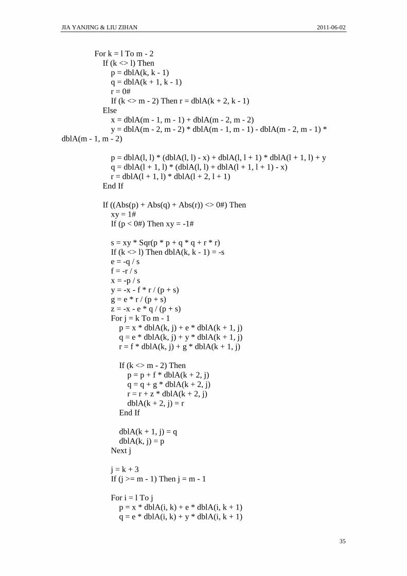
Appendix II: Computation of Maximum Eigenvalue of Normal matrix and Consistence Ratio This section of VBA code enables user to calculate eigenvalues of the pairwise

comparison matrix and choose the maximum eigenvalue to compute consistence ratio.

First the normal pairwise comparison matrix is converted to Hessenberg matrix and

QR method is adapted.


31

'Define variables

Dim Bmat() As Double

Dim dblUR() As Double

Dim dblUI() As Double

ReDim Bmat(n, n) As Double

For i = 1 To n

For j = 1 To n

Bmat(i, j) = Imat(i, j)

Next

Next

Call MHberg(n, Bmat)

ReDim dblUR(n)

ReDim dblUI(n)

Dim maxEigen As Double

Dim CI As Double

Dim s As String

If MHbergEigenv(n, Bmat(), dblUR, dblUI, 0.000001, 10) Then

For i = 1 To n

s = dblUR(i) & " " & dblUI(i) & "i" & Chr(13) & s

If dblUR(i) > maxEigen And dblUI(i) = 0 Then

maxEigen = Round(dblUR(i), 4)

Else

End If

Next i

End If

'Perform Consistence ratio calculation'

CI = (maxEigen - n) / (n - 1)

Dim CR As Double

CR = CI / RI

'Display result'

lblCR.Caption = " "

lblCR.Caption = Round(CR, 4)

If CR > 0.1 Then

lblWarning.Caption = "Consistence ratio is too large. " & "Please type in the

value and calculate again!"

cmdOK.Enabled = False

Else

lblWarning.Caption = "Consistence ratio is OK!"

cmdOK.Enabled = True


32

End If

'Refersh memory'

For i = 1 To n

Colsum(i) = 0

mat2(i) = 0

Rmat(i) = 0

dblUR(i) = 0

dblUI(i) = 0

For j = 1 To n

Mat1(i, j) = 0

Imat(i, j) = 0

Next

Next

maxEigen = 0

CI = 0

RI = 0

CR = 0

End Sub

'Change the ordinary matrix to Hessen Berg matrix'

Private Sub MHberg(n As Integer, mtxA() As Double)

Dim i As Integer

Dim j As Integer

Dim k As Integer

Dim d As Double

Dim t As Double

For k = 2 To n - 1

d = 0#

For j = k To n

t = mtxA(j, k - 1)

If (Abs(t) > Abs(d)) Then

d = t

i = j

End If

Next j

If (Abs(d) + 1# <> 1#) Then

If (i <> k) Then

For j = k - 1 To n

t = mtxA(i, j)

mtxA(i, j) = mtxA(k, j)

mtxA(k, j) = t

Next j

For j = 1 To n

t = mtxA(j, i)

mtxA(j, i) = mtxA(j, k)


33

mtxA(j, k) = t

Next j

End If

For i = k + 1 To n

t = mtxA(i, k - 1) / d

mtxA(i, k - 1) = 0#

For j = k To n

mtxA(i, j) = mtxA(i, j) - t * mtxA(k, j)

Next j

For j = 1 To n

mtxA(j, k) = mtxA(j, k) + t * mtxA(j, i)

Next j

Next i

End If

Next k

End Sub

'Calculate eigenvalues of Hessen Berg matrix''

Function MHbergEigenv(n As Integer, dblA() As Double, dblUR() As Double, dblUI()

As Double, eps As Double, nMaxItNum As Integer) As Boolean

Dim i As Integer

Dim j As Integer

Dim k As Integer

Dim l As Integer

Dim m As Integer

Dim it As Integer

Dim b As Double

Dim c As Double

Dim w As Double

Dim g As Double

Dim xy As Double

Dim p As Double

Dim q As Double

Dim r As Double

Dim x As Double

Dim s As Double

Dim e As Double

Dim f As Double

Dim z As Double

Dim y As Double

it = 0

m = n + 1

While (m <> 1)


34

l = m - 1

While ((l > 1) And (Abs(dblA(l, l - 1)) > eps * (Abs(dblA(l - 1, l - 1)) +

Abs(dblA(l, l)))))

l = l - 1

Wend

If (l = m - 1) Then

dblUR(m - 1) = dblA(m - 1, m - 1)

dblUI(m - 1) = 0#

m = m - 1

it = 0

Else

If (l = m - 2) Then

b = -(dblA(m - 1, m - 1) + dblA(m - 2, m - 2))

c = dblA(m - 1, m - 1) * dblA(m - 2, m - 2) - dblA(m - 1, m - 2) * dblA(m -

2, m - 1)

w = b * b - 4# * c

y = Sqr(Abs(w))

If (w > 0#) Then

xy = 1#

If (b < 0#) Then xy = -1#

dblUR(m - 1) = (-b - xy * y) / 2#

dblUR(m - 2) = c / dblUR(m - 1)

dblUI(m - 1) = 0#

dblUI(m - 2) = 0#

Else

dblUR(m - 1) = -b / 2#

dblUR(m - 2) = dblUR(m - 1)

dblUI(m - 1) = y / 2#

dblUI(m - 2) = -dblUI(m - 1)

End If

m = m - 2

it = 0

Else

If (it >= nMaxItNum) Then

MHbergEigenv = False

Exit Function

End If

it = it + 1

For j = l + 2 To m - 1

dblA(j, j - 2) = 0#

Next j

For j = l + 3 To m - 1

dblA(j, j - 3) = 0#

Next j


35

For k = l To m - 2

If (k <> l) Then

p = dblA(k, k - 1)

q = dblA(k + 1, k - 1)

r = 0#

If (k <> m - 2) Then r = dblA(k + 2, k - 1)

Else

x = dblA(m - 1, m - 1) + dblA(m - 2, m - 2)

y = dblA(m - 2, m - 2) * dblA(m - 1, m - 1) - dblA(m - 2, m - 1) *

dblA(m - 1, m - 2)

p = dblA(l, l) * (dblA(l, l) - x) + dblA(l, l + 1) * dblA(l + 1, l) + y

q = dblA(l + 1, l) * (dblA(l, l) + dblA(l + 1, l + 1) - x)

r = dblA(l + 1, l) * dblA(l + 2, l + 1)

End If

If ((Abs(p) + Abs(q) + Abs(r)) <> 0#) Then

xy = 1#

If (p < 0#) Then xy = -1#

s = xy * Sqr(p * p + q * q + r * r)

If (k <> l) Then dblA(k, k - 1) = -s

e = -q / s

f = -r / s

x = -p / s

y = -x - f * r / (p + s)

g = e * r / (p + s)

z = -x - e * q / (p + s)

For j = k To m - 1

p = x * dblA(k, j) + e * dblA(k + 1, j)

q = e * dblA(k, j) + y * dblA(k + 1, j)

r = f * dblA(k, j) + g * dblA(k + 1, j)

If (k <> m - 2) Then

p = p + f * dblA(k + 2, j)

q = q + g * dblA(k + 2, j)

r = r + z * dblA(k + 2, j)

dblA(k + 2, j) = r

End If

dblA(k + 1, j) = q

dblA(k, j) = p

Next j

j = k + 3

If (j >= m - 1) Then j = m - 1

For i = l To j

p = x * dblA(i, k) + e * dblA(i, k + 1)

q = e * dblA(i, k) + y * dblA(i, k + 1)


36

r = f * dblA(i, k) + g * dblA(i, k + 1)

If (k <> m - 2) Then

p = p + f * dblA(i, k + 2)

q = q + g * dblA(i, k + 2)

r = r + z * dblA(i, k + 2)

dblA(i, k + 2) = r

End If

dblA(i, k + 1) = q

dblA(i, k) = p

Next i

End If

Next k

End If

End If

Wend

MHbergEigenv = True

End Function

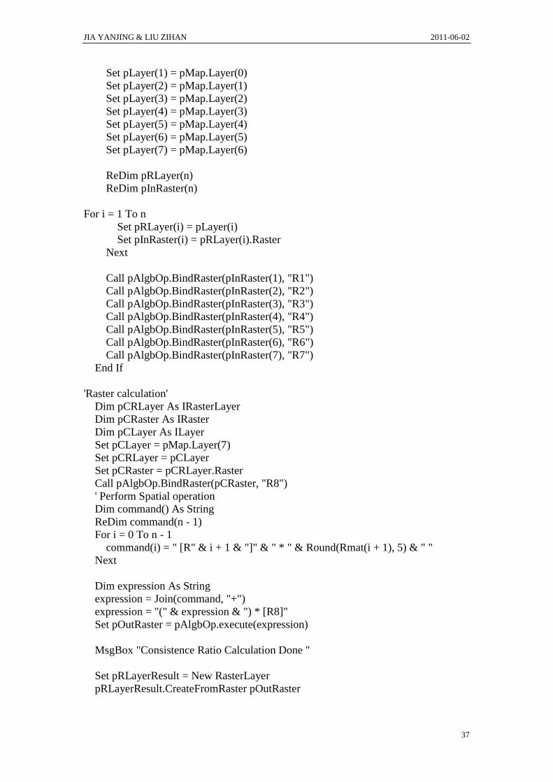
Appendix III: Final result map generation This part of VBA code enable user to create and add raster layers. In this case, the

default n equals to 7 and the system acquire layer according to their priority.

Dim i As Integer

Dim j As Integer

Dim n As Integer

Dim RI As Single

Set pMxDoc = ThisDocument

Set pMap = pMxDoc.FocusMap

' Create a Spatial operator

Dim pAlgbOp As IMapAlgebraOp

Set pAlgbOp = New RasterMapAlgebraOp

' Set output workspace

Dim pEnv As IRasterAnalysisEnvironment

Set pEnv = pAlgbOp

Dim pWS As IWorkspace

Dim pWSF As IWorkspaceFactory

Set pWSF = New RasterWorkspaceFactory

Set pWS = pWSF.OpenFromFile("H:\Final_thesis\result2", 0)

Set pEnv.OutWorkspace = pWS

ReDim pLayer(n)


37

Set pLayer(1) = pMap.Layer(0)







ReDim pRLayer(n)

ReDim pInRaster(n)

For i = 1 To n

Set pRLayer(i) = pLayer(i)

Set pInRaster(i) = pRLayer(i).Raster

Next

Call pAlgbOp.BindRaster(pInRaster(1), "R1")







End If

'Raster calculation'

Dim pCRLayer As IRasterLayer

Dim pCRaster As IRaster

Dim pCLayer As ILayer

Set pCLayer = pMap.Layer(7)

Set pCRLayer = pCLayer

Set pCRaster = pCRLayer.Raster

Call pAlgbOp.BindRaster(pCRaster, "R8")

' Perform Spatial operation

Dim command() As String

ReDim command(n - 1)

For i = 0 To n - 1

command(i) = " [R" & i + 1 & "]" & " * " & Round(Rmat(i + 1), 5) & " "

Next

Dim expression As String

expression = Join(command, "+")

expression = "(" & expression & ") * [R8]"

Set pOutRaster = pAlgbOp.execute(expression)

MsgBox "Consistence Ratio Calculation Done "

Set pRLayerResult = New RasterLayer

pRLayerResult.CreateFromRaster pOutRaster

using multi-criteria analysis and gis to determine the …431811/fulltext01.pdfexamensarbete,...

Documents