MNRAS 491, 2506–2519 (2020) doi:10.1093/mnras/stz3097Advance Access publication 2019 November 6

Using machine learning to study the kinematics of cold gas in galaxies

James M. Dawson,1‹ Timothy A. Davis ,1 Edward L. Gomez,1,2 Justus Schock,3

Nikki Zabel1 and Thomas G. Williams 1

1School of Physics and Astronomy, Cardiff University, The Parade, Cardiff CF24 3AA, UK2Las Cumbres Observatory, Suite 102, 6740 Cortona Dr, Goleta, CA 93117, USA3RWTH Aachen University, Templergraben 55, D-52062 Aachen, Germany

Accepted 2019 October 31. Received 2019 October 31; in original form 2019 June 21

ABSTRACTNext generation interferometers, such as the Square Kilometre Array, are set to obtain vastquantities of information about the kinematics of cold gas in galaxies. Given the volume ofdata produced by such facilities astronomers will need fast, reliable, tools to informativelyfilter and classify incoming data in real time. In this paper, we use machine learning techniqueswith a hydrodynamical simulation training set to predict the kinematic behaviour of cold gas ingalaxies and test these models on both simulated and real interferometric data. Using the powerof a convolutional autoencoder we embed kinematic features, unattainable by the human eyeor standard tools, into a 3D space and discriminate between disturbed and regularly rotatingcold gas structures. Our simple binary classifier predicts the circularity of noiseless, simulated,galaxies with a recall of 85% and performs as expected on observational CO and H I velocitymaps, with a heuristic accuracy of 95%. The model output exhibits predictable behaviourwhen varying the level of noise added to the input data and we are able to explain the roles ofall dimensions of our mapped space. Our models also allow fast predictions of input galaxies’position angles with a 1σ uncertainty range of ±17◦ to ±23◦ (for galaxies with inclinationsof 82.5◦ to 32.5◦, respectively), which may be useful for initial parametrization in kinematicmodelling samplers. Machine learning models, such as the one outlined in this paper, may beadapted for SKA science usage in the near future.

Key words: galaxies: evolution – galaxies: kinematics and dynamics – galaxies: statistics.

1 IN T RO D U C T I O N

The age of Big Data is now upon us; with the Square KilometreArray (SKA) and Large Synoptic Survey Telescope (LSST) bothset to see first light in the mid-2020s.

A key area for big data in the next decades will be the studyingof the kinematics of cold gas in galaxies beyond our own. Thisfield will rely on interferometers, such as the SKA, thanks to theirability to reveal the morphology and kinematics of the cold gasat high spatial and spectral resolution. Current instruments likethe Atacama Large Millimeter/submillimeter Array (ALMA) haverevolutionized the study of gas in galaxies with their sensitive, highresolution, observations of gas kinematics. However, this field lacksthe benefits afforded by fast survey instruments, having long beenin an era of point and shoot astronomy. As such, large data setscapable of containing global statistics in this research domain haveyet to emerge and studies are plagued by slow analytical methodswith high user-involvement.

� E-mail: dawsonj5@cardiff.ac.uk

At the time of writing, large-scale radio interferometric surveyssuch as WALLABY (Duffy et al. 2012) and APERTIF (Oosterloo,Verheijen & van Cappellen 2010) are set to begin and will motivatethe creation of tools that are scalable to survey requirements.However, these tools will be insufficient for screening objects comethe advent of next-generation instruments which are set to receiveenormous quantities of data, so large in fact that storing raw databecomes impossible.

In recent times, disc instabilities, feedback, and major/minormergers have become favoured mechanisms for morphologicalevolution of galaxies (e.g. Parry, Eke & Frenk 2009; Bournaudet al. 2011; Sales et al. 2012), the effects of which are visible intheir gas kinematics. Therefore, gas kinematics could be used torapidly identify interesting structures and events suitable for under-standing drivers of galaxy evolution (e.g. Diaz et al. 2019). If thekinematics of galaxies can accurately yield information on feedbackprocesses and major/minor merger rates, then astronomers usingnext generation instruments could develop a better understandingof which mechanisms dominate changes in star formation propertiesand morphology of galaxies. In order to do this we must developfast, robust, kinematic classifiers.

C© 2019 The Author(s)Published by Oxford University Press on behalf of the Royal Astronomical Society

Dow

nloaded from https://academ

ic.oup.com/m

nras/article-abstract/491/2/2506/5613962 by Acquisitions user on 29 January 2020

Machine learning and cold gas kinematics 2507

Recently, machine learning (ML) has been used successfully inastronomy for a range of tasks including gravitational wave detec-tion (e.g. Shen et al. 2017; Zevin et al. 2017; Gabbard et al. 2018;George & Huerta 2018), exoplanet detection (e.g. Shallue & Van-derburg 2018), analysing photometric light-curve image sequences(e.g. Carrasco-Davis et al. 2019), and used extensively in studies ofgalaxies (e.g. Dieleman, Willett & Dambre 2015; Ackermann et al.2018; Domınguez Sanchez et al. 2018a,b; Bekki 2019).

While using ML requires large data acquisition, training time,resources, and the possibility of results that are difficult to interpret,the advantages of using ML techniques over standard tools include(but are not limited to) increased test speed, higher empiricalaccuracy, and the removal of user-bias. These are all ideal qualitieswhich suit tool-kits for tackling hyperlarge data sets. However,the use of ML on longer wavelength millimetre and radio galaxysources has been absent, with the exception of a few test cases (e.g.Alger et al. 2018; Ma et al. 2018; Andrianomena, Rafieferantsoa &Dave 2019), with the use of such tests to study the gas kinematicsof galaxies being non-existent. It is therefore possible that, in theage of big data, studying gas kinematics with ML could stand as atool for improving interferometric survey pipelines and encouragingresearch into this field before the advent of the SKA.

Cold gas in galaxies that is unperturbed by environmental orinternal effects will relax in a few dynamical times. In this state, thegas forms a flat disc, rotating in circular orbits about some centre ofpotential, to conserve angular momentum. Any disturbance to thegas causes a deviation from this relaxed state and can be observedin the galaxy’s kinematics. Ideally therefore, one would like to beable to determine the amount of kinetic energy of the gas investedin circular rotation (the so-called circularity of the gas; Saleset al. 2012). Unfortunately this cannot be done empirically fromobservations because an exact calculation of circularity requiresfull 6D information pertaining to the 3D positions and velocities ofa galaxy’s constituent components. Instead, in the past, astronomershave used approaches such as radial and Fourier fitting routines (e.g.Krajnovic et al. 2006a; Spekkens & Sellwood 2007; Bloom et al.2017) or 2D power-spectrum analyses (e.g. Grand et al. 2015) todetermine the kinematic regularity of gas velocity fields.

In this work we use an ML model, called a convolutional autoen-coder, and a hydrodynamical simulation training set to predict thecircularity of the cold interstellar medium in galaxies. We test ourresulting model on both simulated test data and real interferometricobservations. We use the power of convolutional neural networksto identify features unattainable by the human eye or standardtools and discriminate between levels of kinematic disorder ofgalaxies. With this in mind, we create a binary classifier to predictwhether the cold gas in galaxies exhibit dispersion-dominated ordisc-dominated rotation in order to maximize the recall of raregalaxies with disturbed cold gas.

In Section 1.1 we provide the necessary background informationfor understanding what ML models we use throughout this paper.In Section 2.1 we describe the measuring of kinematic regularityof gas in galaxies and how it motivates the use of ML in our work.In Section 2 we outline our preparation of simulated galaxies intoa learnable training set as well as the ML methods used to predictcorresponding gas kinematics. In Section 3 the results of the trainingprocess are presented and discussed with a variety of observationaltest cases. Finally, in Section 4 we explain our conclusions andpropose further avenues of research.

1.1 Background to convolutional autoencoders

Convolutional neural networks (CNNs), originally named neocog-nitrons during their infancy (Fukushima 1980), are a special classof neural network (NN) used primarily for classifying multichannelinput matrices, or images. Information is derived from raw pixels,negating the need for a user-involved feature extraction stage; theresult being a hyperparametric model with high empirical accuracy.Today, they are used for a range of problems from medical imagingto driverless cars.

A conventional CNN can have any number of layers (and costlyoperations) including convolutions, max-pooling, activations, fullyconnected layers, and outputs and often utilize regularizationtechniques to reduce overfitting. (For a more in depth background tothe internal operations of CNNs we refer the reader to Krizhevsky,Sutskever & Hinton 2012). These networks are only trainable(through back propagation) thanks to the use of modern graphicsprocessing units (GPUs; Steinkraus, Buck & Simard 2005). It isbecause of access to technology such as GPUs that we are ableto explore the use of ML in a preparatory fashion for instrumentscience with the SKA in this paper.

A CNN will train on data by minimizing the loss between sampledinput images and a target variables. Should training require samplingfrom a very large data set, training on batches of inputs (also calledmini-batches) can help speed up training times by averaging theloss between input and target over a larger sample of inputs. Shouldthe network stagnate in minimizing the loss, reducing the learningrate can help the network explore a minimum over the parameterspace of learnable weights and thus increase the training accuracy.Both of the aforementioned changes to the standard CNN trainingprocedure are used in our models throughout this paper.

An autoencoder is a model composed of two subnets, an en-coder and a decoder. Unlike a standard CNN, during training,an autoencoder learns to reduce the difference between input andoutput vectors rather than the difference between output vectorand target label (whether this be a continuous or categorical setof target classes). In an undercomplete autoencoder the encodersubnet extracts features and reduces input images to a constrainednumber of nodes. This so-called bottleneck forces the network toembed useful information about the input images into a non-linearmanifold from which the decoder subnet reconstructs the inputimages and is scored against the input image using a loss function.With this in mind, the autoencoder works similar to a powerfulnon-linear generalization of principal component analysis (PCA),but rather than attempting to find a lower dimensional hyperplane,the model finds a continuous non-linear latent surface on which thedata best lies.

Autoencoders have been used, recently, in extragalactic astron-omy for de-blending sources (Reiman & Gohre 2019) and imagegeneration of active galactic nuclei (AGNs; Ma et al. 2018).

A convolutional autoencoder (CAE) is very similar to a standardautoencoder but the encoder is replaced with a CNN featureextraction subnet and the decoder is replaced with a transposedconvolution subnet. This allows images to be passed to the CAErather than 1D vectors and can help interpret extracted featuresthrough direct 2D visualization of the convolution filters. For anintuitive explanation of transposed convolutions we direct the readerto Dumoulin & Visin (2016) but for this paper we simply describea transpose convolution as a reverse, one-to-many, convolution.

MNRAS 491, 2506–2519 (2020)

Dow

nloaded from https://academ

ic.oup.com/m

nras/article-abstract/491/2/2506/5613962 by Acquisitions user on 29 January 2020

2508 J. M. Dawson et al.

2 ME T H O D O L O G Y

2.1 Circularity parameter

As described previously, in order to find and classify kinematicdisturbances one would like to measure the circularity of a galaxy’sgas disc. For an object composed of point sources (e.g. molecularclouds, stars, etc.), with known positions, masses, and velocities,the circularity measure

κ = Krot

Kwhere Krot =

N∑i=1

1

2mi

(jz,i

Ri

)2

and K =N∑

i=1

1

2miv

2i ,

(1)

analyses the fraction of kinetic energy invested in circular, ordered,rotation (Sales et al. 2012). Here, Krot is a measure of the rotationalkinetic energy about some axis and K is the total kinetic energy ofthe object. m, j, R, and v represent the mass, angular momentum,radius from the centre of rotation, and velocity of each point inan object, respectively. Objects with perfectly circular, disc like,rotation have κ = 1, while objects with either entirely randommotion or no motion at all have κ = 0.

As κ can only be calculated empirically from simulated galaxies,combining ML techniques with simulations will allow us to exploretheir abilities to learn features that can be used to recover κ inobservations faster, and more robustly, than by human eye. In fact, κhas been used in previous studies to infer the origin of galaxy stellarmorphologies (Sales et al. 2012) and, more recently, to investigatethe kinematics of gas in post starburst galaxies (Davis et al. 2019).

2.2 EAGLE

The Evolution and Assembly of GaLaxies and their Environments(EAGLE) project1 is a collection of cosmological hydrodynamicalsimulations which follow the evolution of galaxies and blackholes in a closed volume � cold dark matter (�CDM) universe.The simulations boast subgrid models which account for physicalprocesses below a known resolution limit (Crain et al. 2015; Schayeet al. 2015; The EAGLE team 2017). These simulations are able toreproduce high levels of agreement with a range of galaxy propertieswhich take place below their resolution limits (see e.g. Schayeet al. 2015). Each simulation was conducted using smooth particlehydrodynamics, meaning users can directly work with the simulateddata in the form of particles, whose properties are stored in outputfiles and a data base that can be queried.

In this paper we make use of these simulations, in conjunctionwith kinematic modelling tools, to generate a learnable training set.We then probe the use of this training set for transfer learning withthe primary goal being to recover kinematic features from generatedvelocity maps. Using simulations has certain advantages overcollecting real data including accessibility, larger sample sizes, andthe ability to calculate empirical truths from the data. However, thereare drawbacks, including: unproven model assumptions, imperfectphysics, and trade-off between resolution and sample size due tocomputational constraints.

The scripts for reading in data, from the EAGLE project database, were adapted versions of the EAGLE team’s pre-writtenscripts.2 The original simulations are saved into 29 snapshots for

1http://icc.dur.ac.uk/Eagle/2https://github.com/jchelly/read eagle

redshifts z = 0–20 and for this work we utilize snapshot 28 forRefL0025N0376 and RefL050N0752 and snapshots 28, 27,26, and 25 for RefL0100N1504 (i.e. redshifts z = 0–0.27). Whenselecting galaxies from these snapshots, we set lower limits on thetotal gas mass (>1 × 109 M�) and stellar mass (>5 × 109 M�)within an aperture size of 30 kpc around each galaxy’s centre ofpotential (i.e. the position of the most bound particle considering allmass components), in order to exclude dwarf galaxies. In order toselect particles which are representative of cold, dense, moleculargas capable of star formation, we only accepted particles with aSFR > 0 for pre-processing (as described in Section 2.3). Thereare many ways to select cold gas in the EAGLE simulations (Lagoset al. 2015) but we use this method for its simplicity as our primarygoal is to create a model that is capable of learning low-levelkinematic features so as to generalize well in transfer learningtests. The upper radial limit for particle selection of 30 kpc, fromthe centre of potential, is in keeping with the scales over whichinterferometers, such as ALMA, typically observe low-redshiftgalaxies. It is important that we replicate these scales in order to testour model performance with real data as described in Section 3.3.One should note that for future survey instruments, such as the SKA,an alternative scaling via consideration of noise thresholds wouldbe more appropriate. However, as we are particularly interestedin the performance of our models with ALMA observations, weinstead impose a radial limit for this work. At this stage we also seta lower limit on the number of particles within the 30 kpc apertureto >200. This was to ensure we had enough particles to calculatestatistically valid kinematic properties of the galaxies and reducescaling issues caused by clipping pixels with low brightness whengenerating velocity maps. With these selection criteria, we workwith a set of 14 846 simulated galaxies.

2.3 Data preparation

Each galaxy was rotated so that their total angular momentum vectorwas aligned with the positive z-axis using the centre of potential (asdefined in the EAGLE Data base; see The EAGLE team 2017) as theorigin. We then made use of the Python based kinematic simulatorKinMS3 (KINematic Molecular Simulation) from Davis et al.(2013) to turn EAGLE data into mock interferometric observations.KinMS has flexibility in outputting astronomical data cubes (withposition, position, and frequency dimensions) and moment mapsfrom various physical parametrizations and has been used for COmolecular gas modelling in previous work (e.g. Davis et al. 2013)and for observational predictions from EAGLE (Davis et al. 2019).Using KinMS we generate simulated interferometric observationsof galaxies directly from their 3D particle distributions.

Thanks to the controllable nature of the EAGLE data, we havethe ability to generate millions of images from just a handful ofsimulations by using combinations of rotations and displacementsof thousands of simulated galaxies per snapshot. This flexibility alsohas the added benefit of naturally introducing data augmentationfor boosting the generalizing power of an ML algorithm. For anygiven distance projection, galaxies were given eight random integerrotations in position-angle (0◦ ≤ θpos < 360◦) and inclination (5◦ ≤φinc ≤ 85◦). Each galaxy is displaced such that they fill a 64 arcsec ×64 arcsec mock velocity map image in order to closely reflect thefield of view (FOV) when observing CO(1-0) line emission withALMA. We define the displacement of each simulated galaxy in

3https://github.com/TimothyADavis/KinMSpy

MNRAS 491, 2506–2519 (2020)

Dow

nloaded from https://academ

ic.oup.com/m

nras/article-abstract/491/2/2506/5613962 by Acquisitions user on 29 January 2020

Machine learning and cold gas kinematics 2509

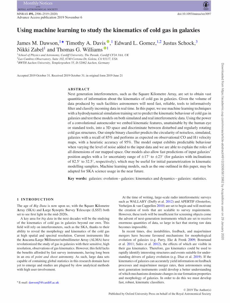
Figure 1. Random exemplar velocity maps for the noiseless EAGLE dataset. Rows of increasing order, starting from the bottom of the figure, showgalaxies of increasing κ . The κ for each galaxy is shown in the bottom rightof the frame in a grey box. Each galaxy has randomly selected position angleand inclination and the colourbar indicates the line of sight velocities, whichhave been normalized into the range −1 to 1 and subsequently denoted aspixel values. The images have dimensions of 64 × 64 pixels in keepingwith the size of input images to our models in this paper, as described inSection 2.6. One can easily see the changes in velocity field from κ ∼ 1 toκ ∼ 0 as galaxies appear less disc-like with more random velocities.

terms of their physical size and desired angular extent. Each galaxy’sradius is given as the 98th percentile particle distance from its centreof potential in kpc. We use this measurement, rather than the truemaximum particle radius, to reduce the chance of selecting sparselypopulated particles for calculating displacement distances, as theycan artificially scale down galaxies.

The EAGLE galaxies were passed to KinMS to create cubesof stacked velocity maps, with fixed mock beam sizes of bmaj =3 arcsec, ready for labelling. Each cube measured 64 × 64 × 8where 64 × 64 corresponds to the image dimensions (in pixels) andeight corresponds to snapshots during position-angle and inclinationrotations. The median physical scale covered by each pixel across allimage cubes in a representative sample of our training set is 0.87 kpc.It should be noted that we set all non-numerical values or infinitiesto a constant value, as passing such values to an ML algorithm willbreak its training. We adopt 0 km s−1 as our constant (similarly toDiaz et al. 2019) to minimize the background influencing featureextraction. Our training set has a range in blank fraction (i.e. thefraction of pixels in images with blank values set to 0 km s−1) of 0.14to 0.98, with a median blank fraction of 0.52. Fig. 1 shows simulatedALMA observations of galaxies when using KinMS in conjunctionwith particle data from the EAGLE simulation RefL0025N0376.

2.4 Simulating noise

Often it is useful to observe the performance of ML models whenadding noise to the input data, in order to test their robustnessand their behavioural predictability. In one of our tests, we seededthe mock-EAGLE-interferometric-data cubes with Gaussian dis-tributed noise of mean μ = 0 and standard deviation

σ = 1

S/N

(1

N

c=N∑c=0

Imax,c

), (2)

Figure 2. A histogram of κ labelled galaxies in the noiseless EAGLEtraining set. Galaxies have been binned in steps of δκ = 0.1 for visualizationpurposes but remain continuous throughout training and testing. Thedistribution of κ is heavily imbalanced, showing that more galaxies exhibita κ closer to 1 than 0.

i.e. some fraction, 1S/N , of the mean maximum intensity, Imax, of

each cube-channel, c, containing line emission. The resulting noisydata cubes are then masked using smooth masking, a method thatis representative of how one would treat a real data cube (Dame2011). An intensity weighted moment one map is then generated inKinMS from the masked cube as

M1 =∫

(v)Ivdv∫Ivdv

=∑

(v)Iv∑Iv

, (3)

where Iv is the observed intensity in a channel with known velocityv, before being normalized into the range of −1 to 1.

Noise presents a problem when normalizing images into thepreferred range. Rescaling, using velocities beyond the range of realvalues in a velocity map (i.e. scaling based on noise), will artificiallyscale down the true values and thus galaxies will appear to exhibitvelocities characteristic of lower inclinations. We clip all noisymoment 1 maps at a fixed 96th percentile level, before normalizing,in order to combat this effect. Note that this choice of clipping atthe 96th percentile level is arbitrarily based on a handful of testcases and represents no specific parameter optimization. Althoughsimple, this likely reflects the conditions of a next generation surveyin which clipping on the fly will be done using a predeterminedmethod globally rather than optimizing on a case by case basis.

2.5 Labelling the training set

Each galaxy, and therefore every cube, is assigned a label in thecontinuous range of 0 to 1 corresponding to the level of orderedrotation, κ , of that galaxy.

In Fig. 1, the difference between levels of κ is clear in bothstructure and velocity characteristics, with low κ galaxies exhibitingless regular structures and more disturbed velocity fields than highκ galaxies.

Fig. 2 shows the distribution of κ in our training set. It is clearthat our training set is heavily imbalanced with a bias towardsthe presence of high κ galaxies. Additionally, as κ approachesone, the possible variation in velocity fields decreases as thereare limited ways in which one can create orderly rotating disc-like structures. However, our data set contains a surplus of galaxiesas κ approaches one. Therefore, if one were to randomly sample

MNRAS 491, 2506–2519 (2020)

Dow

nloaded from https://academ

ic.oup.com/m

nras/article-abstract/491/2/2506/5613962 by Acquisitions user on 29 January 2020

2510 J. M. Dawson et al.

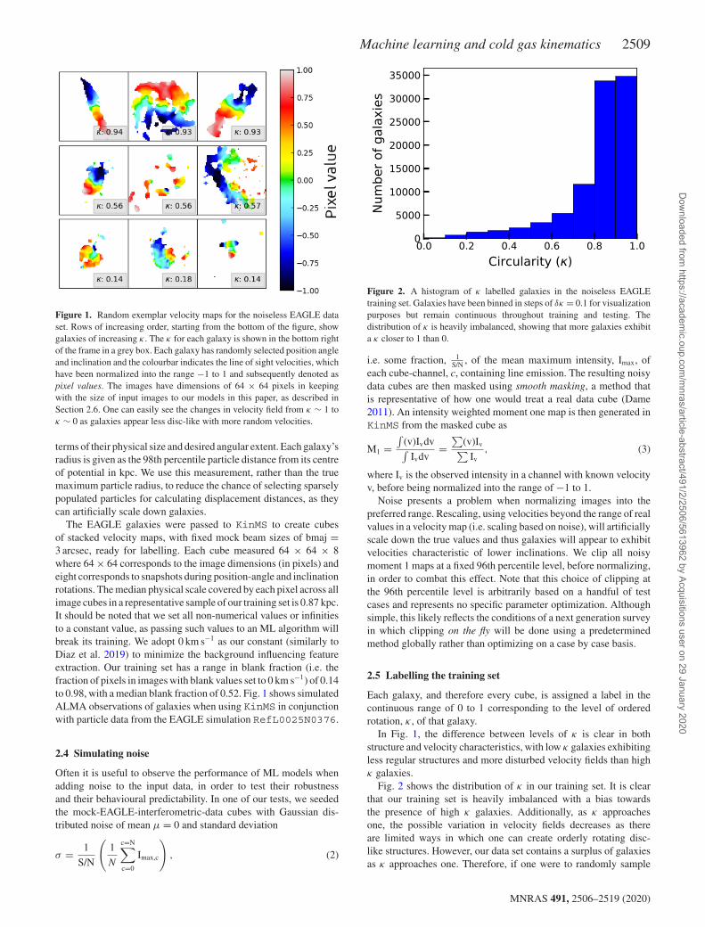
Figure 3. Illustration of the CAE architecture used in this paper. The encoder subnet (top) makes use of a series of convolutions and max-pooling operationsto embed input image information into three latent dimensions. The decoder subnet (bottom) recovers the input image using transposed convolutions andup-sampling layers. The output of the encoder is passed to the decoder during training but throughout testing only the encoder is used map velocity maps intolatent space.

from our data set, for training an ML model, then the model wouldundoubtedly overfit to high κ images. This is a common problemin ML particularly with outlier detection models whose objectivesare to highlight the existence of rare occurrences. In Section 2.6we describe our solution for this problem with the use of weightedsampling throughout training to balance the number of galaxieswith underrepresented κ values seen at each training epoch.

2.6 Model training: Rotationally invariant case

In this section we describe the creation and training of a convolu-tional autoencoder to embed κ into latent space and build a binaryclassifier to separate galaxies with κ above and below 0.5. Note that0.5 is an arbitrarily chosen threshold for our classification boundarybut is motivated by the notion of separating ordered from disturbedgas structures in galaxies.

In order to construct our ML model, we make use of PyTorch4

0.4.1, an open source ML library capable of GPU accelerated tensorcomputation and automatic differentiation (Paszke et al. 2017).Being grounded in Python, PyTorch is designed to be linear andintuitive for researchers with a C99 API backend for competitivecomputation speeds. We use PyTorch due to its flexible and userfriendly nature for native Python users.

A visual illustration of the CAE architecture is shown in Fig. 3and described in Table A1 in more detail. The model follows no hardstructural rules and is an adaption of standard CNN models. Thedecoder structure is simply a reflection of the encoder for simplicity.This means our CAE is unlikely to have the most optimizedarchitecture and we propose this as a possible avenue for improving

4http://pytorch.org/

on the work presented in this paper. The code developed for thispaper is available on GitHub5 as well as an ongoing developmentversion.6

The CAE is trained for 300 epochs (with a batch size of 32) whereone epoch comprises a throughput of 6400 images sampled fromthe training set. We do this to reduce the memory load throughouttraining given such a large training set. Images are selected foreach mini-batch using a weighted sampler which aims to balancethe number of images in each κ bin of width δκ = 0.1. Inputs aresampled with replacement allowing multiple sampling of objectsto prevent under-filled bins. The model uses a mean squared error(MSE) loss,

L = 1

N

N∑i=0

(f (xi) − yi)2, (4)

for evaluating the error between input and output images andweights are updated through gradient descent. N, f(x), and y denotethe batch size, model output for an input x, and target respectively.We use an adaptive Adam learning rate optimizer (Kingma & Ba2014), starting with a learning rate of 0.001 which halves every30 epochs; this helps to reduce stagnation in the model accuracyfrom oversized weight updates. In Fig. 4 we see that the model hasconverged well before the 300th epoch and observe no turnover ofthe test MSE loss, which would indicate overfitting.

The CAE learned to encode input images to 3D latent vectors.Further testing showed that any higher compression, to lowerdimensions, resulted in poor performance for the analyses describedin Section 3 and compression to higher dimensions impaired our

5https://github.com/SpaceMeerkat/CAE/releases/tag/v1.0.06https://github.com/SpaceMeerkat/CAE

MNRAS 491, 2506–2519 (2020)

Dow

nloaded from https://academ

ic.oup.com/m

nras/article-abstract/491/2/2506/5613962 by Acquisitions user on 29 January 2020

Machine learning and cold gas kinematics 2511

Figure 4. Training the CAE on noiseless EAGLE velocity maps. The solidlines show the natural log mean MSE loss and solid colour regions show 1σ

spread at any given epoch. In order to reduce computational time, the testaccuracy is evaluated every 10th epoch. We see smooth convergence of ourCAE throughout training with no turnover of the test accuracy indicatingthat our model did not overfit to the training data.

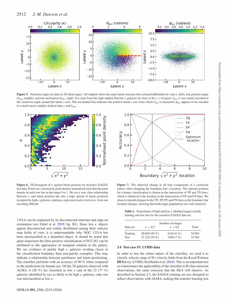
ability to directly observe correlations between features and latentpositions with no improvement to the model’s performance. Weuse scikit-learn’s7 PCA function on these vectors to rotatethe latent space so that it aligns with one dominant latent axis, inthis case the z axis. As seen in Fig. 5, the 3D latent space containsstructural symmetries which are not needed when attempting torecover κ (but are still astrophysically useful; see Section 3.5).Because of this, the data are folded around the z and x axesconsecutively to leave a 2D latent space devoid of structuralsymmetries with dimensions |z| and

√x2 + y2 from which we

could build our classifier (see Section 3.3).Having tested multiple classifiers on the 2D latent space (such as

high-order polynomial and regional boundary approaches), we findthat a simple vertical boundary line is best at separating the galaxieswhose κ are greater than or less than 0.5. This is highlighted in Fig. 6,where we see the spread on latent positions taken up by differentκ galaxies makes a regression to recover κ too difficult. In order tooptimize the boundary line location, we measure the true positive(TP), true negative (TN), false positive (FP), and false negative (FN)scores when progressively increasing the boundary line’s x location.The intersection of TP and TN lines (and therefore the FP and FNlines) in Fig. 7 indicates the optimal position for our boundary,which is at

√x2 + y2 = 2.961 ± 0.002. The smoothness of the

lines in Fig. 7 show how the two κ populations are well structured.If the two populations were clumpy and overlapping, one wouldobserve unstable lines as the ratio of positive and negatively labelledgalaxies constantly shifts in an unpredictable manner.

3 R ESULTS AND DISCUSSION

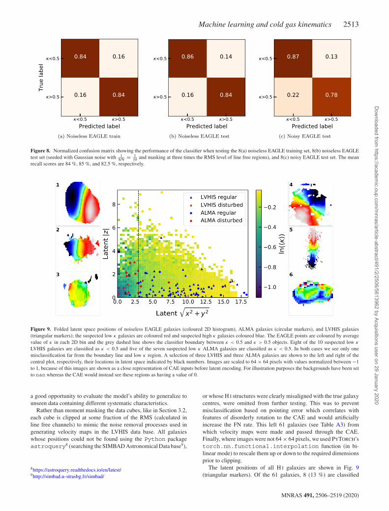
3.1 Test case I: Noiseless EAGLE data

The number of high and low κ labelled images, in both the trainingand test sets, for the noiseless EAGLE data set are shown in Table 1.Fig. 8(a) shows the classification accuracy on the noiseless EAGLEtraining set. The TP and TN accuracy scores are unsurprisingly

7https://scikit-learn.org/

identical given the method used to find the optimal boundary inSection 2.6 was designed to achieve this (see intersection points inFig. 7). The classifier has a mean training recall of 84 % for bothclasses.

Fig. 8(b) shows the confusion matrix when testing the noiselessEAGLE test set using our boundary classifier. We see that themodel performs slightly better than when tested on the trainingset, suggesting that the model did not overfit to the training data andis still able to encode information on κ for unseen images.

3.2 Test case II: Noisy EAGLE data

Fig. 8(c) shows the results of classifying noisy EAGLE test data withS/N = 10 and masking at three times the RMS level (see Section 2.4for details). Note that this is a simple test case and places no majorsignificance on the particular level of S/N used. The introductionof noise has a clear and logical, yet arguably minor, impact onthe classifier’s accuracy. The combination of adding noise followedby using an arbitrary clipping level causes test objects to gravitatetowards the low κ region in latent space. This should come as nosurprise as κ correlates with ordered motion; therefore, any leftover noise from the clipping procedure, which itself appears asdisorderly motions and structures in velocity maps, anticorrelateswith κ causing a systematic shift towards the low κ region in latentspace.

One could reduce this shifting to low κ regions in several ways.(1) Removing low S/N galaxies from the classification sample. (2)For our test cases we used a single absolute percentile level forsmooth clipping noise; using levels optimized for cases on a one-by-one basis will prevent overclipping. (3) If one were to directlysample the noise properties from a specific instrument, seeding thesimulated training data with this noise before retraining an CAEwould cause a systematic shift in the boundary line, mitigating aloss in accuracy. It should also be noted that we have not tested thelower limit of S/N for which it is appropriate to use our classifierbut instead we focus on demonstrating the effects of applying noiseclipping globally across our test set under the influence of modestnoise.

3.3 Test case III: ALMA data

We tested 30 velocity maps of galaxies observed with ALMA toevaluate the performance of the classifier on real observations.Given that we used KinMS to tailor the simulated velocity mapsto closely resemble observations with ALMA we expect similarbehaviour as seen when testing the simulated data. For our testsample we use an aggregated selection of 15 velocity maps fromthe mm-Wave Interferometric Survey of Dark Object Masses(WISDOM) CO(1-0, 2-1, and 3-2) and 15 CO(1-0) velocity mapsfrom the ALMA Fornax Cluster Survey (AlFoCS; Zabel et al.2019). We classify each galaxy, by eye, as either disturbed orregularly rotating (see Table A2) in order to heuristically evaluatethe classifier’s performance.

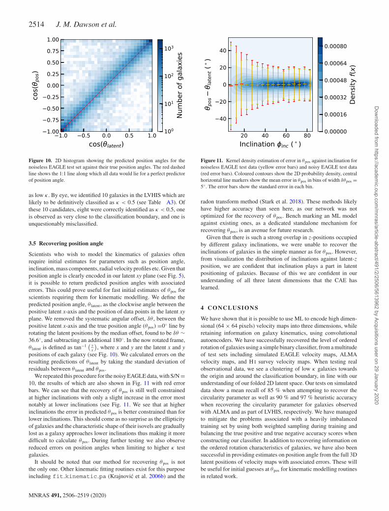
Fig. 9 shows the positions of all ALMA galaxies (round markers)in our folded latent space, once passed through the CAE. Of the 30galaxies, 6 (20 %) are classified as κ < 0.5; this higher fraction,when compared to the fraction of low κ galaxies in the simulatedtest set, is likely due to the high number of dwarf galaxies, withirregular H2 gas, targeted in AlFoCS.

We find one false positive classification close to the classifica-tion boundary and one false positive classification far from theclassification boundary. The false negative classification of NGC

MNRAS 491, 2506–2519 (2020)

Dow

nloaded from https://academ

ic.oup.com/m

nras/article-abstract/491/2/2506/5613962 by Acquisitions user on 29 January 2020

2512 J. M. Dawson et al.

Figure 5. Noiseless eagle test data in 3D latent space. All subplots show the same latent structure but coloured differently by: true κ (left), true position angle(θpos, middle), and true inclination (φinc, right). It is clear from the right subplot that low κ galaxies lie close to the z = 0 region. θpos is very neatly encoded inthe clockwise angle around the latent z-axis. The red dashed line indicates the positive latent x axis from which θpos is measured. φinc appears to be encodedin a much more complex fashion than κ and θpos.

Figure 6. 2D histogram of κ against latent position for noiseless EAGLEtest data. Pixels are coloured by point density normalized such that the pointdensity in each row lies in the range 0 to 1. We see a very clear relationshipbetween κ and latent position but also a high spread of latent positionsoccupied by high κ galaxies, making a regression task to recover κ from ourencoding difficult.

1351A can be explained by its disconnected structure and edge-onorientation (see Zabel et al. 2019; fig. B1). Since low κ objectsappear disconnected and widely distributed among their velocitymap fields of view, it is understandable why NGC 1351A hasbeen misclassified as a disturbed object. It should be noted thatupon inspection the false positive classification of FCC282 can beattributed to the appearance of marginal rotation in the galaxy.We see evidence of patchy high κ galaxies residing closer tothe classification boundary than non-patchy examples. This mayindicate a relationship between patchiness and latent positioning.The classifier performs with an accuracy of 90 % when comparedto the predictions by human eye. Of the 30 galaxies observed withALMA, 6 (20 %) are classified as low κ and of the 23 (77 %)galaxies identified by eye as likely to be high κ galaxies, only onewas misclassified as low κ .

Figure 7. The observed change in all four components of a confusionmatrix when changing the boundary line x-location. The optimal positionfor a binary classification is chosen as the intersection of TP and TN lines,which is identical to the location at the intersection of FP and FN lines. Weobserve smooth changes to the TN, TP, FP, and FN lines as the boundary linelocation changes, showing that both target populations are well clustered.

Table 1. Proportions of high and low κ labelled images in bothtraining and test sets for the noiseless EAGLE data set.

Number of imagesData set κ > 0.5 κ < 0.5 Total

Training 88 840 (94 %) 6144 (6 %) 94 984Test 22 224 (93 %) 1560 (7 %) 23 784

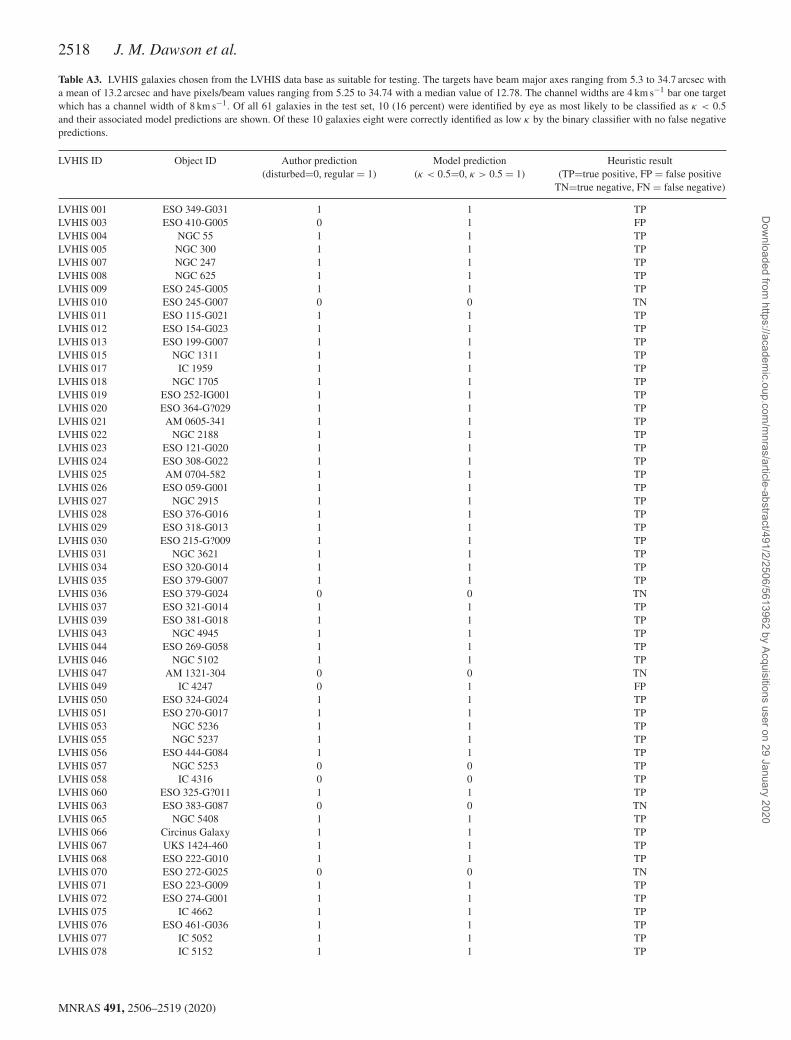
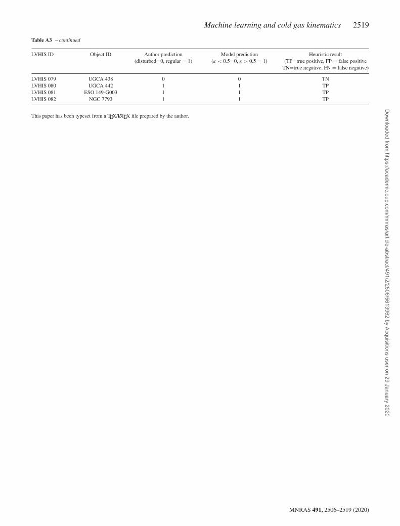
3.4 Test case IV: LVHIS data

In order to test the robust nature of the classifier, we used it toclassify velocity maps of H I velocity fields from the Local VolumeHI Survey (LVHIS; Koribalski et al. 2018). This is an important testas it determines the applicability of the classifier to H I line emissionobservations, the same emission that the SKA will observe. Asdescribed in Section 2.3, the EAGLE training set was designed toreflect observations with ALMA, making this transfer learning test

MNRAS 491, 2506–2519 (2020)

Dow

nloaded from https://academ

ic.oup.com/m

nras/article-abstract/491/2/2506/5613962 by Acquisitions user on 29 January 2020

Machine learning and cold gas kinematics 2513

(a) Noiseless EAGLE train (b) Noiseless EAGLE test (c) Noisy EAGLE test

Figure 8. Normalized confusion matrix showing the performance of the classifier when testing the 8(a) noiseless EAGLE training set, 8(b) noiseless EAGLEtest set (seeded with Gaussian noise with 1

S/N = 110 and masking at three times the RMS level of line free regions), and 8(c) noisy EAGLE test set. The mean

recall scores are 84 %, 85 %, and 82.5 %, respectively.

Figure 9. Folded latent space positions of noiseless EAGLE galaxies (coloured 2D histogram), ALMA galaxies (circular markers), and LVHIS galaxies(triangular markers); the suspected low κ galaxies are coloured red and suspected high κ galaxies coloured blue. The EAGLE points are coloured by averagevalue of κ in each 2D bin and the grey dashed line shows the classifier boundary between κ < 0.5 and κ > 0.5 objects. Eight of the 10 suspected low κ

LVHIS galaxies are classified as κ < 0.5 and five of the seven suspected low κ ALMA galaxies are classified as κ < 0.5. In both cases we see only onemisclassification far from the boundary line and low κ region. A selection of three LVHIS and three ALMA galaxies are shown to the left and right of thecentral plot, respectively, their locations in latent space indicated by black numbers. Images are scaled to 64 × 64 pixels with values normalized between −1to 1, because of this images are shown as a close representation of CAE inputs before latent encoding. For illustration purposes the backgrounds have been setto nan whereas the CAE would instead see these regions as having a value of 0.

a good opportunity to evaluate the model’s ability to generalize tounseen data containing different systematic characteristics.

Rather than moment masking the data cubes, like in Section 3.2,each cube is clipped at some fraction of the RMS (calculated inline free channels) to mimic the noise removal processes used ingenerating velocity maps in the LVHIS data base. All galaxieswhose positions could not be found using the Python packageastroquery8 (searching the SIMBAD Astronomical Data base9),

8https://astroquery.readthedocs.io/en/latest/9http://simbad.u-strasbg.fr/simbad/

or whose H I structures were clearly misaligned with the true galaxycentres, were omitted from further testing. This was to preventmisclassification based on pointing error which correlates withfeatures of disorderly rotation to the CAE and would artificiallyincrease the FN rate. This left 61 galaxies (see Table A3) fromwhich velocity maps were made and passed through the CAE.Finally, where images were not 64 × 64 pixels, we used PYTORCH’storch.nn.functional.interpolation function (in bi-linear mode) to rescale them up or down to the required dimensionsprior to clipping.

The latent positions of all H I galaxies are shown in Fig. 9(triangular markers). Of the 61 galaxies, 8 (13 %) are classified

MNRAS 491, 2506–2519 (2020)

Dow

nloaded from https://academ

ic.oup.com/m

nras/article-abstract/491/2/2506/5613962 by Acquisitions user on 29 January 2020

2514 J. M. Dawson et al.

Figure 10. 2D histogram showing the predicted position angles for thenoiseless EAGLE test set against their true position angles. The red dashedline shows the 1:1 line along which all data would lie for a perfect predictorof position angle.

as low κ . By eye, we identified 10 galaxies in the LVHIS which arelikely to be definitively classified as κ < 0.5 (see Table A3). Ofthese 10 candidates, eight were correctly identified as κ < 0.5, oneis observed as very close to the classification boundary, and one isunquestionably misclassified.

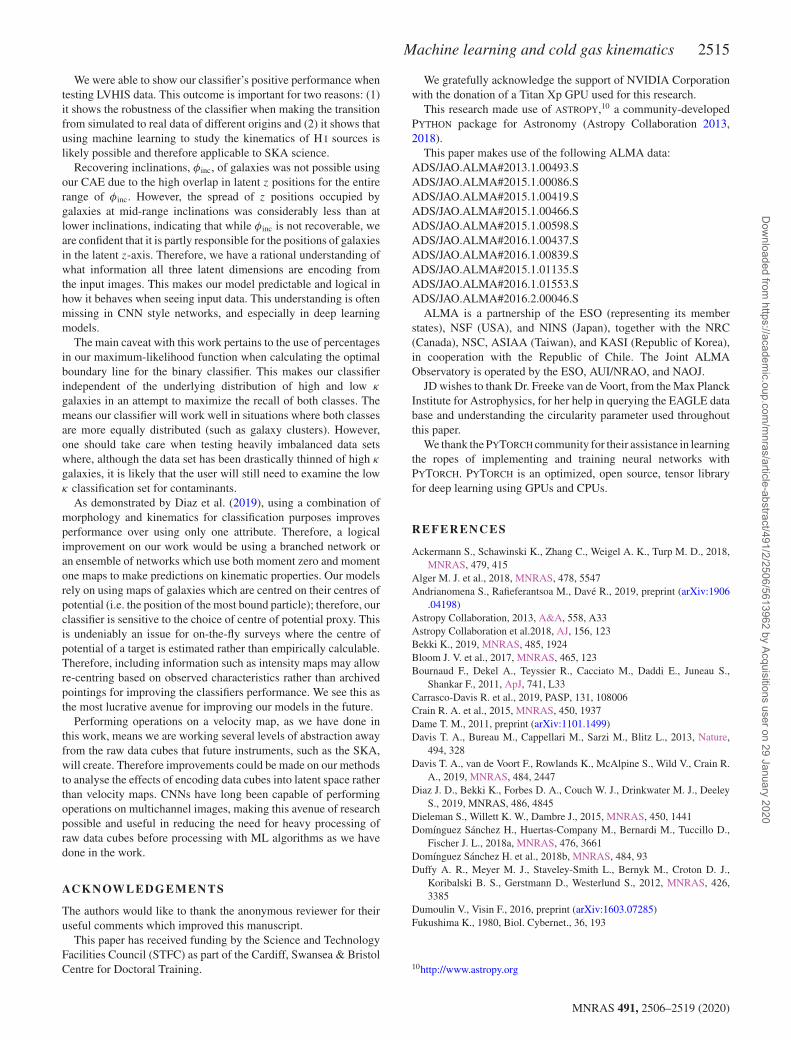
3.5 Recovering position angle

Scientists who wish to model the kinematics of galaxies oftenrequire initial estimates for parameters such as position angle,inclination, mass components, radial velocity profiles etc. Given thatposition angle is clearly encoded in our latent xy plane (see Fig. 5),it is possible to return predicted position angles with associatederrors. This could prove useful for fast initial estimates of θpos forscientists requiring them for kinematic modelling. We define thepredicted position angle, θ latent, as the clockwise angle between thepositive latent x-axis and the position of data points in the latent xyplane. We removed the systematic angular offset, δθ , between thepositive latent x-axis and the true position angle (θpos) =0◦ line byrotating the latent positions by the median offset, found to be δθ ∼36.6◦, and subtracting an additional 180◦. In the now rotated frame,θ latent is defined as tan−1

(y

x

), where x and y are the latent x and y

positions of each galaxy (see Fig. 10). We calculated errors on theresulting predictions of θ latent by taking the standard deviation ofresiduals between θ latent and θpos.

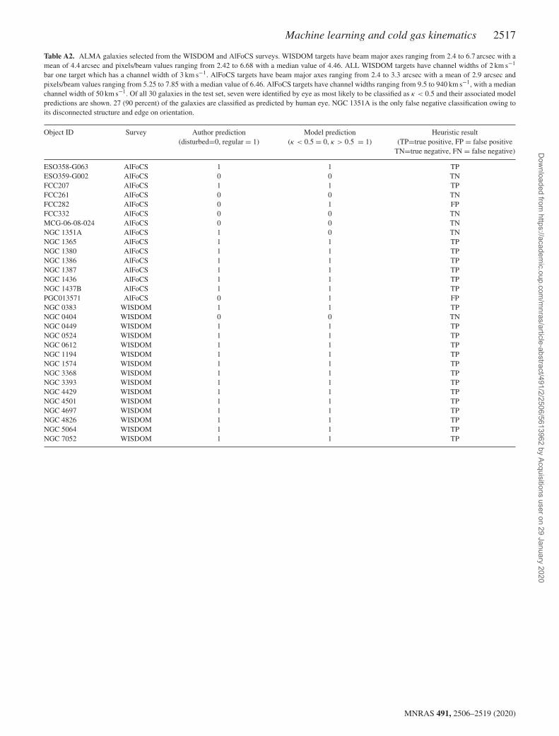
We repeated this procedure for the noisy EAGLE data, with S/N =10, the results of which are also shown in Fig. 11 with red errorbars. We can see that the recovery of θpos is still well constrainedat higher inclinations with only a slight increase in the error mostnotably at lower inclinations (see Fig. 11. We see that at higherinclinations the error in predicted θpos is better constrained than forlower inclinations. This should come as no surprise as the ellipticityof galaxies and the characteristic shape of their isovels are graduallylost as a galaxy approaches lower inclinations thus making it moredifficult to calculate θpos. During further testing we also observereduced errors on position angles when limiting to higher κ testgalaxies.

It should be noted that our method for recovering θpos is notthe only one. Other kinematic fitting routines exist for this purposeincluding fit kinematic pa (Krajnovic et al. 2006b) and the

Figure 11. Kernel density estimation of error in θpos against inclination fornoiseless EAGLE test data (yellow error bars) and noisy EAGLE test data(red error bars). Coloured contours show the 2D probability density, centralhorizontal line markers show the mean error in θpos in bins of width δθpos =5◦. The error bars show the standard error in each bin.

radon transform method (Stark et al. 2018). These methods likelyhave higher accuracy than seen here, as our network was notoptimized for the recovery of θpos. Bench marking an ML modelagainst existing ones, as a dedicated standalone mechanism forrecovering θpos, is an avenue for future research.

Given that there is such a strong overlap in z-positions occupiedby different galaxy inclinations, we were unable to recover theinclinations of galaxies in the simple manner as for θpos. However,from visualization the distribution of inclinations against latent-zposition, we are confident that inclination plays a part in latentpositioning of galaxies. Because of this we are confident in ourunderstanding of all three latent dimensions that the CAE haslearned.

4 C O N C L U S I O N S

We have shown that it is possible to use ML to encode high dimen-sional (64 × 64 pixels) velocity maps into three dimensions, whileretaining information on galaxy kinematics, using convolutionalautoencoders. We have successfully recovered the level of orderedrotation of galaxies using a simple binary classifier, from a multitudeof test sets including simulated EAGLE velocity maps, ALMAvelocity maps, and H I survey velocity maps. When testing realobservational data, we see a clustering of low κ galaxies towardsthe origin and around the classification boundary, in line with ourunderstanding of our folded 2D latent space. Our tests on simulateddata show a mean recall of 85 % when attempting to recover thecircularity parameter as well as 90 % and 97 % heuristic accuracywhen recovering the circularity parameter for galaxies observedwith ALMA and as part of LVHIS, respectively. We have managedto mitigate the problems associated with a heavily imbalancedtraining set by using both weighted sampling during training andbalancing the true positive and true negative accuracy scores whenconstructing our classifier. In addition to recovering information onthe ordered rotation characteristics of galaxies, we have also beensuccessful in providing estimates on position angle from the full 3Dlatent positions of velocity maps with associated errors. These willbe useful for initial guesses at θpos for kinematic modelling routinesin related work.

MNRAS 491, 2506–2519 (2020)

Dow

nloaded from https://academ

ic.oup.com/m

nras/article-abstract/491/2/2506/5613962 by Acquisitions user on 29 January 2020

Machine learning and cold gas kinematics 2515

We were able to show our classifier’s positive performance whentesting LVHIS data. This outcome is important for two reasons: (1)it shows the robustness of the classifier when making the transitionfrom simulated to real data of different origins and (2) it shows thatusing machine learning to study the kinematics of H I sources islikely possible and therefore applicable to SKA science.

Recovering inclinations, φinc, of galaxies was not possible usingour CAE due to the high overlap in latent z positions for the entirerange of φinc. However, the spread of z positions occupied bygalaxies at mid-range inclinations was considerably less than atlower inclinations, indicating that while φinc is not recoverable, weare confident that it is partly responsible for the positions of galaxiesin the latent z-axis. Therefore, we have a rational understanding ofwhat information all three latent dimensions are encoding fromthe input images. This makes our model predictable and logical inhow it behaves when seeing input data. This understanding is oftenmissing in CNN style networks, and especially in deep learningmodels.

The main caveat with this work pertains to the use of percentagesin our maximum-likelihood function when calculating the optimalboundary line for the binary classifier. This makes our classifierindependent of the underlying distribution of high and low κ

galaxies in an attempt to maximize the recall of both classes. Themeans our classifier will work well in situations where both classesare more equally distributed (such as galaxy clusters). However,one should take care when testing heavily imbalanced data setswhere, although the data set has been drastically thinned of high κ

galaxies, it is likely that the user will still need to examine the lowκ classification set for contaminants.

As demonstrated by Diaz et al. (2019), using a combination ofmorphology and kinematics for classification purposes improvesperformance over using only one attribute. Therefore, a logicalimprovement on our work would be using a branched network oran ensemble of networks which use both moment zero and momentone maps to make predictions on kinematic properties. Our modelsrely on using maps of galaxies which are centred on their centres ofpotential (i.e. the position of the most bound particle); therefore, ourclassifier is sensitive to the choice of centre of potential proxy. Thisis undeniably an issue for on-the-fly surveys where the centre ofpotential of a target is estimated rather than empirically calculable.Therefore, including information such as intensity maps may allowre-centring based on observed characteristics rather than archivedpointings for improving the classifiers performance. We see this asthe most lucrative avenue for improving our models in the future.

Performing operations on a velocity map, as we have done inthis work, means we are working several levels of abstraction awayfrom the raw data cubes that future instruments, such as the SKA,will create. Therefore improvements could be made on our methodsto analyse the effects of encoding data cubes into latent space ratherthan velocity maps. CNNs have long been capable of performingoperations on multichannel images, making this avenue of researchpossible and useful in reducing the need for heavy processing ofraw data cubes before processing with ML algorithms as we havedone in the work.

AC K N OW L E D G E M E N T S

The authors would like to thank the anonymous reviewer for theiruseful comments which improved this manuscript.

This paper has received funding by the Science and TechnologyFacilities Council (STFC) as part of the Cardiff, Swansea & BristolCentre for Doctoral Training.

We gratefully acknowledge the support of NVIDIA Corporationwith the donation of a Titan Xp GPU used for this research.

This research made use of ASTROPY,10 a community-developedPYTHON package for Astronomy (Astropy Collaboration 2013,2018).

This paper makes use of the following ALMA data:ADS/JAO.ALMA#2013.1.00493.SADS/JAO.ALMA#2015.1.00086.SADS/JAO.ALMA#2015.1.00419.SADS/JAO.ALMA#2015.1.00466.SADS/JAO.ALMA#2015.1.00598.SADS/JAO.ALMA#2016.1.00437.SADS/JAO.ALMA#2016.1.00839.SADS/JAO.ALMA#2015.1.01135.SADS/JAO.ALMA#2016.1.01553.SADS/JAO.ALMA#2016.2.00046.S

ALMA is a partnership of the ESO (representing its memberstates), NSF (USA), and NINS (Japan), together with the NRC(Canada), NSC, ASIAA (Taiwan), and KASI (Republic of Korea),in cooperation with the Republic of Chile. The Joint ALMAObservatory is operated by the ESO, AUI/NRAO, and NAOJ.

JD wishes to thank Dr. Freeke van de Voort, from the Max PlanckInstitute for Astrophysics, for her help in querying the EAGLE database and understanding the circularity parameter used throughoutthis paper.

We thank the PYTORCH community for their assistance in learningthe ropes of implementing and training neural networks withPYTORCH. PYTORCH is an optimized, open source, tensor libraryfor deep learning using GPUs and CPUs.

REFERENCES

Ackermann S., Schawinski K., Zhang C., Weigel A. K., Turp M. D., 2018,MNRAS, 479, 415

Alger M. J. et al., 2018, MNRAS, 478, 5547Andrianomena S., Rafieferantsoa M., Dave R., 2019, preprint (arXiv:1906

.04198)Astropy Collaboration, 2013, A&A, 558, A33Astropy Collaboration et al.2018, AJ, 156, 123Bekki K., 2019, MNRAS, 485, 1924Bloom J. V. et al., 2017, MNRAS, 465, 123Bournaud F., Dekel A., Teyssier R., Cacciato M., Daddi E., Juneau S.,

Shankar F., 2011, ApJ, 741, L33Carrasco-Davis R. et al., 2019, PASP, 131, 108006Crain R. A. et al., 2015, MNRAS, 450, 1937Dame T. M., 2011, preprint (arXiv:1101.1499)Davis T. A., Bureau M., Cappellari M., Sarzi M., Blitz L., 2013, Nature,

494, 328Davis T. A., van de Voort F., Rowlands K., McAlpine S., Wild V., Crain R.

A., 2019, MNRAS, 484, 2447Diaz J. D., Bekki K., Forbes D. A., Couch W. J., Drinkwater M. J., Deeley

S., 2019, MNRAS, 486, 4845Dieleman S., Willett K. W., Dambre J., 2015, MNRAS, 450, 1441Domınguez Sanchez H., Huertas-Company M., Bernardi M., Tuccillo D.,

Fischer J. L., 2018a, MNRAS, 476, 3661Domınguez Sanchez H. et al., 2018b, MNRAS, 484, 93Duffy A. R., Meyer M. J., Staveley-Smith L., Bernyk M., Croton D. J.,

Koribalski B. S., Gerstmann D., Westerlund S., 2012, MNRAS, 426,3385

Dumoulin V., Visin F., 2016, preprint (arXiv:1603.07285)Fukushima K., 1980, Biol. Cybernet., 36, 193

10http://www.astropy.org

MNRAS 491, 2506–2519 (2020)

Dow

nloaded from https://academ

ic.oup.com/m

nras/article-abstract/491/2/2506/5613962 by Acquisitions user on 29 January 2020

2516 J. M. Dawson et al.

Gabbard H., Williams M., Hayes F., Messenger C., 2018, Phys. Rev. Lett.,120, 141103

George D., Huerta E. A., 2018, Phys. Lett. B, 778, 64Grand R. J. J., Bovy J., Kawata D., Hunt J. A. S., Famaey B., Siebert A.,

Monari G., Cropper M., 2015, MNRAS, 453, 1867Kingma D. P., Ba J., 2014, preprint (arXiv:1412.6980)Koribalski B. S. et al., 2018, MNRAS, 478, 1611Krajnovic D., Cappellari M., de Zeeuw P. T., Copin Y., 2006a, MNRAS,

366, 787Krajnovic D., Cappellari M., de Zeeuw P. T., Copin Y., 2006b, MNRAS,

366, 787Krizhevsky A., Sutskever I., Hinton G. E., 2012, in Pereira F., Burges C. J.

C., Bottou L., Weinberger K. Q., eds, Advances in Neural InformationProcessing Systems 25. Curran Associates, Inc., New York, p. 1097.Available at: http://papers.nips.cc/paper/4824-imagenet-classification-with-deep-convolutional-neural-networks.pdf

Lagos C. del P. et al., 2015, MNRAS, 452, 3815Ma Z., Zhu J., Li W., Xu H., 2018, preprint (arXiv:1806.00398)Oosterloo T., Verheijen M., van Cappellen W., 2010, in ISKAF2010 Science

Meeting. p. 43 preprint (arXiv:1007.5141)Parry O. H., Eke V. R., Frenk C. S., 2009, MNRAS, 396, 1972

Paszke A. et al., 2017, in NIPS-WReiman D. M., Gohre B. E., 2019, MNRAS, 485, 2617Sales L. V., Navarro J. F., Theuns T., Schaye J., White S. D. M., Frenk C.

S., Crain R. A., Dalla Vecchia C., 2012, MNRAS, 423, 1544Schaye J. et al., 2015, MNRAS, 446, 521Shallue C. J., Vanderburg A., 2018, AJ, 155, 94Shen H., George D., Huerta E. A., Zhao Z., 2017, preprint (arXiv:1711.099

19)Spekkens K., Sellwood J. A., 2007, ApJ, 664, 204Stark D. V. et al., 2018, MNRAS, 480, 2217Steinkraus D., Buck I., Simard P. Y., 2005, in Eighth International Con-

ference on Document Analysis and Recognition (ICDAR’05), Vol. 2.IEEE, New York, p. 1115

The EAGLE team, 2017, preprint (arXiv:1706.09899)Zabel N. et al., 2019, MNRAS, 483, 2251Zevin M. et al., 2017, Class. Quantum Gravity, 34, 064003

APPENDI X A : INFORMATI ON O N TESTG A L A X I E S

Table A1. Architecture for our autoencoder, featuring both encoder and decoder subnets. The decoder is a direct reflection ofthe encoder’s structure.

Layer Layer type Units/number of filters Size Padding Stride

Encoder Input Input – (64,64) – –Conv1 Convolutional 8 (3,3) 1 1ReLU Activation – – – –Conv2 Convolutional 8 (3,3) 1 1ReLU Activation – – – –MaxPool Max-pooling – (2,2) – 1Conv3 Convolutional 16 (3,3) 1 1ReLU Activation – – – –Conv4 Convolutional 16 (3,3) 1 1ReLU Activation – – – –MaxPool Max-pooling – (2,2) – 1Linear Fully-connected 3 – – –

Decoder Linear Fully-connected 3 – – –Up Partial inverse max-pool – (2,2) – 1ReLU Activation – – – –Trans1 Transposed Convolution 16 (3,3) 1 1ReLU Activation – – – –Trans2 Transposed Convolution 16 (3,3) 1 1Up Partial inverse max-pool – (2,2) – 1ReLU Activation – – – –Trans3 Transposed Convolution 8 (3,3) 1 1ReLU Activation – – – –Trans4 Transposed Convolution 8 (3,3) 1 1Ouput Output – (64,64) – –

MNRAS 491, 2506–2519 (2020)

Dow

nloaded from https://academ

ic.oup.com/m

nras/article-abstract/491/2/2506/5613962 by Acquisitions user on 29 January 2020

Machine learning and cold gas kinematics 2517

Table A2. ALMA galaxies selected from the WISDOM and AlFoCS surveys. WISDOM targets have beam major axes ranging from 2.4 to 6.7 arcsec with amean of 4.4 arcsec and pixels/beam values ranging from 2.42 to 6.68 with a median value of 4.46. ALL WISDOM targets have channel widths of 2 km s−1

bar one target which has a channel width of 3 km s−1. AlFoCS targets have beam major axes ranging from 2.4 to 3.3 arcsec with a mean of 2.9 arcsec andpixels/beam values ranging from 5.25 to 7.85 with a median value of 6.46. AlFoCS targets have channel widths ranging from 9.5 to 940 km s−1, with a medianchannel width of 50 km s−1. Of all 30 galaxies in the test set, seven were identified by eye as most likely to be classified as κ < 0.5 and their associated modelpredictions are shown. 27 (90 percent) of the galaxies are classified as predicted by human eye. NGC 1351A is the only false negative classification owing toits disconnected structure and edge on orientation.

Object ID Survey Author prediction Model prediction Heuristic result(disturbed=0, regular = 1) (κ < 0.5 = 0, κ > 0.5 = 1) (TP=true positive, FP = false positive

TN=true negative, FN = false negative)

ESO358-G063 AlFoCS 1 1 TPESO359-G002 AlFoCS 0 0 TNFCC207 AlFoCS 1 1 TPFCC261 AlFoCS 0 0 TNFCC282 AlFoCS 0 1 FPFCC332 AlFoCS 0 0 TNMCG-06-08-024 AlFoCS 0 0 TNNGC 1351A AlFoCS 1 0 TNNGC 1365 AlFoCS 1 1 TPNGC 1380 AlFoCS 1 1 TPNGC 1386 AlFoCS 1 1 TPNGC 1387 AlFoCS 1 1 TPNGC 1436 AlFoCS 1 1 TPNGC 1437B AlFoCS 1 1 TPPGC013571 AlFoCS 0 1 FPNGC 0383 WISDOM 1 1 TPNGC 0404 WISDOM 0 0 TNNGC 0449 WISDOM 1 1 TPNGC 0524 WISDOM 1 1 TPNGC 0612 WISDOM 1 1 TPNGC 1194 WISDOM 1 1 TPNGC 1574 WISDOM 1 1 TPNGC 3368 WISDOM 1 1 TPNGC 3393 WISDOM 1 1 TPNGC 4429 WISDOM 1 1 TPNGC 4501 WISDOM 1 1 TPNGC 4697 WISDOM 1 1 TPNGC 4826 WISDOM 1 1 TPNGC 5064 WISDOM 1 1 TPNGC 7052 WISDOM 1 1 TP

MNRAS 491, 2506–2519 (2020)

Dow

nloaded from https://academ

ic.oup.com/m

nras/article-abstract/491/2/2506/5613962 by Acquisitions user on 29 January 2020

2518 J. M. Dawson et al.

Table A3. LVHIS galaxies chosen from the LVHIS data base as suitable for testing. The targets have beam major axes ranging from 5.3 to 34.7 arcsec witha mean of 13.2 arcsec and have pixels/beam values ranging from 5.25 to 34.74 with a median value of 12.78. The channel widths are 4 km s−1 bar one targetwhich has a channel width of 8 km s−1. Of all 61 galaxies in the test set, 10 (16 percent) were identified by eye as most likely to be classified as κ < 0.5and their associated model predictions are shown. Of these 10 galaxies eight were correctly identified as low κ by the binary classifier with no false negativepredictions.

LVHIS ID Object ID Author prediction Model prediction Heuristic result(disturbed=0, regular = 1) (κ < 0.5=0, κ > 0.5 = 1) (TP=true positive, FP = false positive

TN=true negative, FN = false negative)

LVHIS 001 ESO 349-G031 1 1 TPLVHIS 003 ESO 410-G005 0 1 FPLVHIS 004 NGC 55 1 1 TPLVHIS 005 NGC 300 1 1 TPLVHIS 007 NGC 247 1 1 TPLVHIS 008 NGC 625 1 1 TPLVHIS 009 ESO 245-G005 1 1 TPLVHIS 010 ESO 245-G007 0 0 TNLVHIS 011 ESO 115-G021 1 1 TPLVHIS 012 ESO 154-G023 1 1 TPLVHIS 013 ESO 199-G007 1 1 TPLVHIS 015 NGC 1311 1 1 TPLVHIS 017 IC 1959 1 1 TPLVHIS 018 NGC 1705 1 1 TPLVHIS 019 ESO 252-IG001 1 1 TPLVHIS 020 ESO 364-G?029 1 1 TPLVHIS 021 AM 0605-341 1 1 TPLVHIS 022 NGC 2188 1 1 TPLVHIS 023 ESO 121-G020 1 1 TPLVHIS 024 ESO 308-G022 1 1 TPLVHIS 025 AM 0704-582 1 1 TPLVHIS 026 ESO 059-G001 1 1 TPLVHIS 027 NGC 2915 1 1 TPLVHIS 028 ESO 376-G016 1 1 TPLVHIS 029 ESO 318-G013 1 1 TPLVHIS 030 ESO 215-G?009 1 1 TPLVHIS 031 NGC 3621 1 1 TPLVHIS 034 ESO 320-G014 1 1 TPLVHIS 035 ESO 379-G007 1 1 TPLVHIS 036 ESO 379-G024 0 0 TNLVHIS 037 ESO 321-G014 1 1 TPLVHIS 039 ESO 381-G018 1 1 TPLVHIS 043 NGC 4945 1 1 TPLVHIS 044 ESO 269-G058 1 1 TPLVHIS 046 NGC 5102 1 1 TPLVHIS 047 AM 1321-304 0 0 TNLVHIS 049 IC 4247 0 1 FPLVHIS 050 ESO 324-G024 1 1 TPLVHIS 051 ESO 270-G017 1 1 TPLVHIS 053 NGC 5236 1 1 TPLVHIS 055 NGC 5237 1 1 TPLVHIS 056 ESO 444-G084 1 1 TPLVHIS 057 NGC 5253 0 0 TPLVHIS 058 IC 4316 0 0 TPLVHIS 060 ESO 325-G?011 1 1 TPLVHIS 063 ESO 383-G087 0 0 TNLVHIS 065 NGC 5408 1 1 TPLVHIS 066 Circinus Galaxy 1 1 TPLVHIS 067 UKS 1424-460 1 1 TPLVHIS 068 ESO 222-G010 1 1 TPLVHIS 070 ESO 272-G025 0 0 TNLVHIS 071 ESO 223-G009 1 1 TPLVHIS 072 ESO 274-G001 1 1 TPLVHIS 075 IC 4662 1 1 TPLVHIS 076 ESO 461-G036 1 1 TPLVHIS 077 IC 5052 1 1 TPLVHIS 078 IC 5152 1 1 TP

MNRAS 491, 2506–2519 (2020)

Dow

nloaded from https://academ

ic.oup.com/m

nras/article-abstract/491/2/2506/5613962 by Acquisitions user on 29 January 2020

Machine learning and cold gas kinematics 2519

Table A3 – continued

LVHIS ID Object ID Author prediction Model prediction Heuristic result(disturbed=0, regular = 1) (κ < 0.5=0, κ > 0.5 = 1) (TP=true positive, FP = false positive

TN=true negative, FN = false negative)

LVHIS 079 UGCA 438 0 0 TNLVHIS 080 UGCA 442 1 1 TPLVHIS 081 ESO 149-G003 1 1 TPLVHIS 082 NGC 7793 1 1 TP

This paper has been typeset from a TEX/LATEX file prepared by the author.

MNRAS 491, 2506–2519 (2020)

Dow

nloaded from https://academ

ic.oup.com/m

nras/article-abstract/491/2/2506/5613962 by Acquisitions user on 29 January 2020