Using inventory to handle risks in the supplyof oil to Nepal

Biju K. Thapalia and Stein W. Wallace and Michal Kaut

in: International Journal of Business Performance and Supply Chain Modelling. See also BIBTEXentry below.

BIBTEX:

@article{ThapaliaEA08,author = {Biju K. Thapalia and Stein W. Wallace and Michal Kaut},title = {Using inventory to handle risks in the supply of oil to {N}epal},journal = {International Journal of Business Performance and Supply Chain Modelling},year = {2009},volume = {1},pages = {41--60},number = {1},doi = {10.1504/IJBPSCM.2009.026265}

}

© 2009 Inderscience Publishers.The original publication is available from the journal’s web page,http://www.inderscience.com/jhome.php?jcode=ijbpscm.Direct link to the article’s page: http://www.inderscience.com/info/inarticle.php?artid=26265.

Document created on August 2, 2013.Cover page generated with CoverPage.sty.

Using inventory to handle risks in the supply of oil to Nepal

Biju Kr. Thapalia∗ Stein W. Wallace† Michal Kaut‡

Molde University College, P.O. Box 2110, NO-6402 Molde, Norway

30 November 2008

Abstract

Nepal’s unique geographical features, frequent political disturbances, strikes, a limited andcomplicated road network, frequent road breakdowns, government interventions as well as avolatile international oil market make the supply chain of Nepal Oil Corporation (NOC) ratherunique. We analyze different risks in the NOC supply chain and discuss what can be done to findinventory strategies that handle these risks without a particular focused on one specific scenario.

Keywords: Supply Chain, Stochastic programming, Uncertainty, Linear programming, Inventory

1 Introduction

Nepal Oil Corporation (NOC), established by the Nepal government in 1970, is a public enterpriseto import, store and distribute petroleum products in the country. NOC maintains monopoly in thismarket. Nepal being a landlocked country, the entire oil procurement is done through India.

Earlier, the supply of oil to Nepal was handled, in a rather random fashion, by a few privatecompanies. To regulate these unplanned purchases as well as the resulting distribution, the Nepalesegovernment established NOC. This monopoly state of NOC was not created to make profit but to haveeffective distribution at reasonable prices for the customers. We can see this from the losses it hassuffered when oil prices increased in the last decade. NOC has over the last five years accumulateda loss of 12 billion rupees (approx 300 million US Dollars). The government has decided to extendloans of 1.7 billion rupees on its guarantee to NOC to pay dues to the Indian supplier. As of June2007, http://ekantipur.com estimated that NOC owes 4.5 billion rupees to the Indian OilCorporation (IOC) . Long queues in front of petrol pumps have become a common phenomenon inKathmandu and in the rest of the country, which is of more concern to the government and to thegeneral customers, than NOC’s losses.

Oil being a sensitive product, NOC finds it difficult to operate efficiently due to government in-terventions. Pricing and procurement are political and bilateral issues, which are dictated by thegovernment and the bilateral agreement between Nepal and India. The major job in NOC is that ofoperational activities which includes storing and distributing oil products. NOC sees possibilities ofimproving its performance by managing the operational activities of its supply chain in a better way.

∗Biju.K.Thapalia@hiMolde.no†Stein.W.Wallace@hiMolde.no‡Michal.Kaut@hiMolde.no

1

The country’s unique geographical features, frequent political disturbances, strikes, limited andcomplicated road network, frequent road breakdowns, government interventions and a volatile inter-national oil market make this supply chain a very complicated one. A study of NOC’s distributionnetwork motivated us to better understand the risks and uncertainties associated with the supply chainand how these can be managed. We shall focus on how long-term inventories can be used to managethe risks. This way of management, being rather standard in general, is particularly involved for acompany consistently short on foreign currencies.

The paper is organized as follows. The next section explains the supply chain of NOC and themajor players in this network; the third section deals with risks in a supply chain. The fourth sectiondwells on a linear programming formulation of NOC’s distribution problem and its possible exten-sions. The fifth deals with a stochastic version of the model and the scenarios are discussed. Thesixth section explains the result of the optimization problem while, finally, the seventh section is theconclusion of the paper.

2 NOC’s supply chain and its distribution network

The supply chain for oil distribution in Nepal is unique in the sense that there are not many players andlevels in this network. The focal company in this analysis does not have full control of the completesupply chain, as it is heavily dependent on the agreement between India and Nepal at government leveland many other external parties. NOC, our focus company, can only increase its efficiency by takingwhat is given and optimize the network from there. The paper focuses on the distribution networkbetween the refineries and depots of the IOC and the depots of NOC.

2.1 The players in NOC’s supply chain

The supply chain starts with the International market where crude oil is bought. The oil market isamong the most volatile commodity markets and is extremely sensitive to international events. Overthe last decade, the international prices have increased from about 18 dollars to around 140 dollars perbarrel, and then dropped to the present level of about 50.

The Indian Oil Corporation buys crude oil and processes it into products. NOC imports oil fromrefineries/depots of IOC situated at different places in India. IOC determines prices for the oil productsthat include costs of crude oil at Kolkata port, the transportation cost to the refineries and the refiningcharges. In particular the refining charges are negotiable. NOC has 12 depots in Nepal with totalstorage capacity of around 70300 kilolitre. Presently NOC fills only 15 to 18 percent of the fullcapacity due to its financial constraints. This covers just a few days of consumption. Nearly 1200trucks, owned by independent transport companies, are on contract to distribute the oil products. Mostof the trucks are under trucks associations, which are mostly at regional level, and they do not like tooperate outside their own regions. There are approximately 1900 independently owned distributionpoints throughout the nation. These points cater to the customers’ demand of all oil products exceptaviation fuel. Aviation fuel is distributed directly by NOC. This network of distributors makes itpossible to reach the end customers of NOC. A population of around 27 million, all dependent on oilin some form, directly or indirectly, puts a lot of pressure on this supply chain. Present total demand ofoil products per year is around 0.8 million kilolitre. Sixty-five percent of the total demand originatesfrom the Kathmandu valley. Overall there is an annual growth rate of around 10 percent in the demandfor petroleum products. The network structure of the supply chain is illustrated in Figure 1.

In Figure 1, refineries are owned by IOC and are situated at different places in India. Presently

2

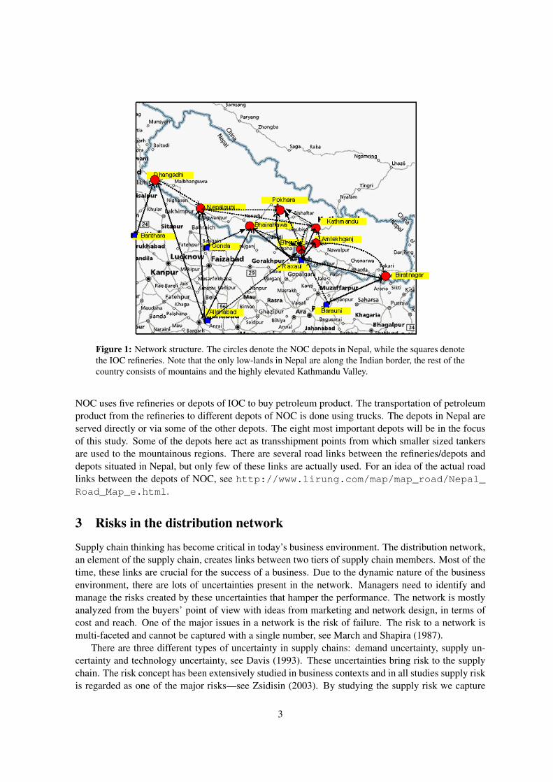
Figure 1: Network structure. The circles denote the NOC depots in Nepal, while the squares denotethe IOC refineries. Note that the only low-lands in Nepal are along the Indian border, the rest of thecountry consists of mountains and the highly elevated Kathmandu Valley.

NOC uses five refineries or depots of IOC to buy petroleum product. The transportation of petroleumproduct from the refineries to different depots of NOC is done using trucks. The depots in Nepal areserved directly or via some of the other depots. The eight most important depots will be in the focusof this study. Some of the depots here act as transshipment points from which smaller sized tankersare used to the mountainous regions. There are several road links between the refineries/depots anddepots situated in Nepal, but only few of these links are actually used. For an idea of the actual roadlinks between the depots of NOC, see http://www.lirung.com/map/map_road/Nepal_Road_Map_e.html.

3 Risks in the distribution network

Supply chain thinking has become critical in today’s business environment. The distribution network,an element of the supply chain, creates links between two tiers of supply chain members. Most of thetime, these links are crucial for the success of a business. Due to the dynamic nature of the businessenvironment, there are lots of uncertainties present in the network. Managers need to identify andmanage the risks created by these uncertainties that hamper the performance. The network is mostlyanalyzed from the buyers’ point of view with ideas from marketing and network design, in terms ofcost and reach. One of the major issues in a network is the risk of failure. The risk to a network ismulti-faceted and cannot be captured with a single number, see March and Shapira (1987).

There are three different types of uncertainty in supply chains: demand uncertainty, supply un-certainty and technology uncertainty, see Davis (1993). These uncertainties bring risk to the supplychain. The risk concept has been extensively studied in business contexts and in all studies supply riskis regarded as one of the major risks—see Zsidisin (2003). By studying the supply risk we capture

3

most of the risk arising from the tangible and intangible features of the supply chain.Meulbrook (2000) defines supply risk as any type of risk that ‘adversely affects inward flow of

any type of resource to enable operations to take place’ whereas Zsidisin, Panelli, and Upton (2000)define supply risk as ‘the transpiration of significant and/or disappointing failures with inbound goodsand service’. Zsidisin (2003), from case studies with purchasing organizations involved in supply riskmanagement, concludes that supply risk can be defined as the probability of an incident associatedwith inbound supply from individual suppliers or the supply market occurring, in which the incidentresults in the inability of the purchasing firm to meet customer demand or causes threats to customerlife and safety.

Most research work on optimization of networks has focused on uncertain demand, but very fewhave analyzed uncertainty from the supply side. This paper analysis risks due to such as randomsupply and arc failures.

The network facing NOC has both intangible and tangible features. The intangible features arethe political relation between the governments of India and Nepal, the international political scenario,the bargaining power of Nepal with India, and Indian foreign policy towards Nepal. The intangiblefeatures of a network are difficult to examine and influence, see Harland, Brencheley, and Walker(2003), but still have profound effects on design decisions and performance of the network. We seethat changes in the government and/or managers, change the relation between the management andthe government which again affects the decision making style. The tangible features are examinable,but they are also to some extent influenced by the intangible features of the network. Thus identifying,defining, and assessing these risks properly for the given network will be a major task.

The breakdown of a source point due to technical fault can be classified as technology uncertainty.In the given case the breakdown in refineries (source point) will result in disruption of supply so thismay also be viewed as a source of supply uncertainty. In the present case the breakdown of anypart of the roads due to any climatic condition or man-made situation can also be regarded as supplyuncertainty. Also political or organizational fallouts may result in blocking or restriction of supplyfrom seller to buyer, which also may be regarded as supply uncertainty.

NOC does not use any linear programming model to plan the supply chain but uses their ex-perience, basic ideas, and simple mathematics to calculate the figures required for ordering, storingand transportation. This model, however, is built in cooperation with NOC, and reflects their way ofthinking. Data was also collected from NOC.

4 Modelling philosophy

There are of course many ways to handle the risks in NOC’s supply chain. Reducing those risks thatare fully or partly man-made will always have a major focus. Our thinking in this paper is somewhatdifferent. We shall focus on long-term inventory, and study how it changes as the different risks(and other model parameters) change for whatever reason. Inventory as a means of handling risksis particularly involved for a company like NOC which is consistently short on foreign currencies,needed to purchase oil from India.

Obviously, the problem of inventory control while purchasing under a limited period-by-periodbudget and random disturbances is an infinite horizon problem. The disturbances occur (mostly)independently of each other, and any disturbance can occur at any point in time. As it stands, thisproblem is not very well suited for stochastic programming. However, we must remember that ourmain issue is long-term inventory control. That is, we would like to understand how inventory shouldbe controlled when everything runs smoothly in expectation of some disturbance. The expectation is

4

Figure 2: Illustration of events with known and random durations (solid lines), the scenario ofno events (dashed line), the period of inventory adjustments (dotted lines), the period of carryinginventory in anticipation of an event (dashed line), and finally the loop.Event 1 has a known duration, while the duration of Event 2 is stochastic: it has a probability of 40%to finish earlier and 60% of lasting longer then Event 1.

that as the probability of disturbances increases, optimal inventory increases, increasing capital costs.So we expect to see the standard trade-off between inventory costs and shortage costs. But the settingis rather different from a simple inventory model.

We shall first make the somewhat common assumption that only one disturbance can occur at anypoint in time. Or in other words, that the probability of two disturbances occurring at the same timeis so low that we can disregard it. In our case, this assumption is critical.

The present model is not an operational model but rather represents a way to explain the effects ofthe different random disturbances on long-term inventory. Figure 2 illustrates our modelling. The ideain the model is that we introduce all random events at a particular point in time (arbitrarily denoted0). At that point inventories and whatever parts of the supply chain that are still working, are used tosupply customers. When the events are over, inventory levels must be brought back to their long-termlevels (which are our main variables) within time t1. Thereafter follow t2 periods of no disturbances.The t2 periods represent where the model will carry the inventory, anticipating the random events.This is the core of the model – carrying inventory in expectation of some disturbance. The longer t2,the less likely is an occurrence. As there is also a scenario representing “no disturbance” we havetwo ways of representing the intensity of disturbances: the choice of t2 and the probability of the nodisturbance scenario. After the model reaches time T = t1 + t2, we loop the model back to the start.This way of looping back can be useful in stochastic models, see for example Lium, Crainic, andWallace (2007).

So we shall end up with a three-stage stochastic programming model. First stage variables shallbe inventory levels in periods of no disturbance, second and third stage variables are all others. Thirdstage variables are associated with events with random durations (like Event 2 in Figure 2). Wecould have let also transportation and purchasing decisions be first stage in the same periods, but havechosen not to: there might be problems of stability of those variables around the end points of thestable periods, and our focus is in any case on the long-term (first-stage) inventories.

It is important to note that the second and third stage variables do not in principle represent oper-ational decisions that can be implemented. The model’s sole focus is on inventories in stable periods.

5

And even more obviously: The elapse of time in the model does not represent the actual flow of time.We believe this formulation of a three stage model for an infinite horizon problem to be a major contri-bution of this paper. Of course, the approach works as well for pure two or multiple stages dependingon the branching structure of the events.

So we conclude this section by repeating the relationship between our problem understanding andour model. In reality, events occur at random points in time, but with known frequencies (data isavailable for many of the events). Whenever one occurs, NOC does its best to supply the countrywith oil using inventory and those parts of the supply chain still functioning. As soon as the eventis over, NOC will try to recover the chosen inventory levels. Those inventories will then be carrieduntil the next event starts. So we see that the less likely the events, the more costly the inventories (inthe sense that they are more rarely used). In the model, the quiet period of length t2 (as well as theno-event scenario) represents when NOC waits for the next event. In the model it is known when theevents occur. But the model is not allowed to take that into account since we force inventories to becarried at stable levels throughout the quiet period. Once an event occurs, the model will try to supplyoil by using inventories and whatever of the supply chain is working. Then, after the event is over,the model forces a rebuild of the inventories, so that they reach the inventories of the stable periodby time t1. Hence, the major variables – the inventories – function the same way in the model as inreality. They are kept in anticipation of events when all is quiet, and used whenever an event occurs.The assumption of no two events taking place at the same time is needed for this modelling to work.In this case this is a reasonable assumption.

5 LP formulation

We formulate the present distribution philosophy of NOC as an LP. This formulation looks into thedistribution of oil products from up to five refineries of IOC in India to a number of depots of NOC inNepal. The objective function minimizes the overall cost of distribution, inventory and penalties fornon-delivery. Following present practice, we always source a depot from the nearest refinery. Sincenot all refineries deliver all products, a given depot might be sourced from several refineries, but therewill never be two refineries sourcing the same product to a given depot. Purchasing of products takesplace in USD. Since the Rupee is not convertible, NOC cannot transfer any amount into USD. Soinstead of having a total budget for all activities, or at least minimizing total costs, we have chosento minimize costs that occur in Rupees under two major constraints: The availability of USD forpurchasing and a requirement that the budget is fully used for purchasing.

We start with a basic LP formulation of the problem when everything is normal. It is a kind ofdeterministic multi-period multi-commodity production and transportation problem with inventory.To address the end-of-horizon problem, we present the model in a circular fashion. This can be donein a simple way by letting the period following period t be (t +1) mod (T +1) and the previousperiod (t +T ) mod (T +1), where 0, . . . ,T are the time periods in the model.1 Since we developthe model in a circular fashion we need not provide initial inventories. The model will itself find theappropriate inventory levels, in fact, that is the purpose of the model. This way we avoid ending upanalyzing the build-up (transient) stage of the operation, which is quite different from the steady-state,which is our focus.

Since NOC is short on foreign currencies, there will be rejection of demand. We represent thatby piece-wise linear penalties. It is crucial not to use simple linear penalties, as that will result in

1There seems to be a disagreement about the interpretation of a mod b if a is negative. Hence, we have chosen to let theperiod preceding period t be (t +T ) mod (T +1) and not (t−1) mod (T +1)

6

unreasonable rejections, such as all demand in a given depot on a given day rejected rather thanrejections spread over depots and time.

The term “node” might need a brief explanation. In the deterministic version of the problem anode represents all decisions associated with a specific time period (day in our case). Hence, if westart counting both nodes and time at zero, the time associated with node n, denoted t(n) is alwaysgiven by t(n)= n. For the stochastic model that will change. We use n and t(n) also in the deterministicformulation to make the transition to the stochastic model as easy as possible.

SetsN NodesD1 Depots that can be reached from their nearest refinery in one day.D2 Depots that can be reached from their nearest refinery in two days.D Set of all depots; D = D1∪D2.I Set of intervals for the piece-wise linear penalty for unsatisfied demand.

Input parametersHk Inventory holding cost per unit of product k per unit of time. As this is mainly

capital costs, it does not depend on j ∈D .Cn

ik Unit cost of transporting product k to depot i (from its nearest refinery).cn

i j Transportation costs between depots i and j inside Nepal.Pk Price of product k, measured in USD.gn

ik Fairness factor (percentage of demand fulfilled) for each product at each depot.dt

ik Demand for product k at depot i at day t.Mik Maximum holding capacity of product k at depot i.B Budget in USD for buying products over the time horizon 0, . . . ,T .U Total capacity of trucks available each day.bl Lengths of intervals for the piece-wise linear penalty; l ∈I

Nik,l Coefficients for the piece-wise linear penalty for product i at depot k; l ∈I .t(n) The time of node n.pa(n) Parent of node n, i.e. the node preceding it. To make the network circular, we set

the parent of the first node to be equal to the last node. This will guarantee thatt(pa(n)

)=(t(n)+T

)mod (T +1).

Decision variables (all depend on n, something that will not be repeated throughout)xn

jk Amount of product k transported to depot j. We use preprocessing to determinewhich refinery will be used. Hence there is no “from” index on x.

wni jk Amount of product k sent from depot i to depot j (both within Nepal)

znik End-of-day inventory of product k at depot i.

qnik Sales of product k at depot i.

rnik,l Rejected demand of product k at depot i, corresponding to the l-th part of the piece-

wise linear penalty; l ∈I .

Then solve

min∑k,n

(∑

jCn

jkxnjk +∑

jHkzn

jk +∑i j

cni jw

ni jk +

3

∑l=1

N jk,l ∑j

rnjk,l

)(1)

7

Subject to

1D1( j)xnjk +1D2( j)xpa(n)

jk + ∑i∈D

wni jk + zpa(n)

jk = qnjk + ∑

i∈Dwn

jik + znjk ∀ j,k,n (2)

∑j∈D

∑k

(xn

jk +∑i

wni jk

)+ ∑

j∈D2

∑k

xpa(n)jk ≤U ∀n (3)

qnjk +∑

iwn

jik ≤ zpa(n)jk ∀ j,k,n (4)

qnjk +

3

∑l=1

rnjk,l = dt(n)

jk ∀ j,k,n (5)

qnjk

dt(n)jk

≥ gnjk

∑m∈N pm∑i∈D qm

ik

∑m∈N pm ∑i∈D dt(m)ik

∀ j,k,n : dt(n)jk > 0 (6)

∑n, j,k

Pk xnjk = B (7)

znjk ≤M jk ∀n, j,k (8)

xnjk,w

ni jk,q

njk,z

njk ≥ 0 ∀n, i, j,k (9)

0≤ rnjk,l ≤ bl dt(n)

jk ∀n, j,k, l ∈I (10)

Here the objective function (1) is the financial representation of the operational activities; the firstcomponent is the cost of transporting oil products to the different depots, the second component isholding costs at different depots (mostly capital costs); the third component shows the inter-depottransportation costs and the last term describes the cost associated with rejecting demand.

Constraints (2) maintain the flow of products in the depots. Here, 1A(x) denotes the indicatorfunction of set A, i.e. it is equal to one if x ∈ A and zero otherwise.

Constraints (3) enforce truck capacity. Here the first part is the truck capacity utilized for all trucksstaring out that day, be that from a refinery or a depot. For depots two days away from the refinerieswe have a second part representing the previous day’s purchases which are on the way.

Constraints (4) say that oil sent to other depots plus oil sold to customers must come from inven-tory. In other words, the incoming volumes xn

jk and wni jk cannot be used the same day they arrive—for

example because they arrive in the evening.Constraints (5) make sure that sales plus rejections add up to demand. Since the rejections are

non-negative, it also ensures that the sales do not exceed the demand.Constraints (6) make sure that we overall treat all depots fairly. Note that the numerator of the

fraction in the right-hand side is equal to the total expected sale of product k, while the denominator isequal to the total demand for the product. Hence, the constraint says that if we satisfy on average p%of the total demand for product k, then we must satisfy at least gn

jk p% of the demand in each depot jand node n.

Constraint (7) shows the limited budget available to NOC to purchase oil from India. This budgetis available in foreign currencies. We use equality as we know that the budget is always too low tosatisfy all demand. As this is a cost minimization model, this is our way of expressing that all salesare worthwhile. These constraints, combined with conservation of flow (2), make sure that all webuy is sold, nothing ends up permanently in inventory. In reality prices vary a bit over refineries.However, had we included that in the model, we would have ended up with a difficulty. Since theNOC budget is not big enough to cover all demand, the model would buy as much oil as possiblein order to avoid penalties for lost demand. And that would mean buying from the cheapest refinery

8

0

1

21

41

61

81

114

134

154

174

207

240

20

40

60

80

100

113

133

153

173

193

206

226

239

259

8788

101

180181

194

213214

227

260 269

0 1 6 7 8 9 15 20 21 30

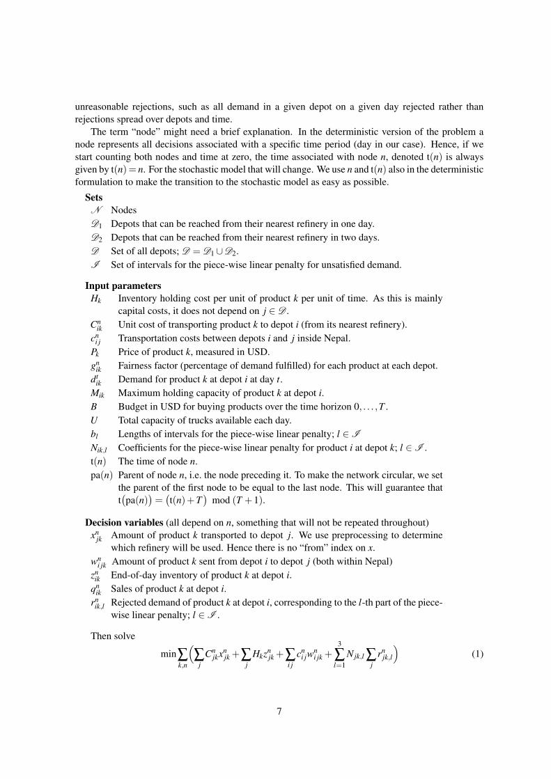
Figure 3: Scenario tree used in the numerical tests. Nodes without displayed numbers are numberedconsecutively from the previous given number. Circles/ellipses represent nodes with an ongoingevent, octagons and diamonds the recovery nodes and finally rectangles represent the normal nodes,i.e. nodes where the inventory is fixed to the steady-state level.

before re-distributing it all over Nepal. This would take place as long as the extra transportation andinventory costs did not outweigh the saved penalties, which they would not in the base case. To avoidthis, which certainly does not describe reality, we use prices Pk which do not vary over refineries,and instead include the differences between depot prices as a part of the transportation cost Cn

jk. Thiseliminates the problem.

Finally, constraints (8) guarantee that the depots will not exceed their holding capacities, con-straints (9) insure non-negative decision variables and constraints (10) limit the size of the rejections.

6 Stochastic LP formulation

The model we develop in this section is a stochastic multi-period model representing the steady-stateof the operation. We use scenarios as outlined in Figure 3, which is a specific case of the more genericFigure 2. Note that because of the looping-back, it is technically not a scenario tree. We will, however,still use some of the scenario-tree terminology and call the nodes in the period before the convergingnodes leaves, even if technically they are not.

At this point we might want to properly define our first-stage variables. Focus then on node260: whatever is the inventory level in node 260 is also enforced during the quiet period (nodes 261through 269, as well as in the no-disturbance scenario: nodes 0 and 114 to 133). Further, the sameinventory is enforced in all leaf nodes. The idea is that after an event is over, the scenario is givensome time to recover from the event, bringing inventories back to “normal” (i.e. that of node 260).

9

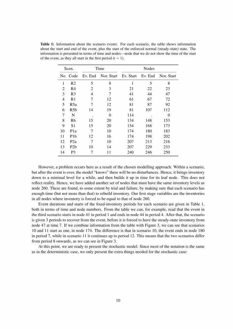
Table 1: Information about the scenario events. For each scenario, the table shows informationabout the start and end of the event, plus the start of the enforced normal (steady-state) state. Theinformation is presented in terms of time and nodes—node that we do not show the time of the startof the event, as they all start in the first period (t = 1).

Scen. Time Nodes

No. Code Ev. End Nor. Start Ev. Start Ev. End Nor. Start

1 R2 5 8 1 5 82 R4 2 3 21 22 233 R3 4 7 41 44 474 R1 7 12 61 67 725 R5a 7 12 81 87 926 R5b 14 19 81 107 1127 N . 0 114 . 08 R6 15 20 134 148 1539 S1 15 20 154 168 173

10 P1a 7 10 174 180 18311 P1b 12 16 174 198 20212 P2a 7 10 207 213 21613 P2b 10 14 207 229 23314 P3 7 11 240 246 250

However, a problem occurs here as a result of the chosen modelling approach. Within a scenario,but after the event is over, the model “knows” there will be no disturbances. Hence, it brings inventorydown to a minimal level for a while, and then builds it up in time for its leaf node. This does notreflect reality. Hence, we have added another set of nodes that must have the same inventory levels asnode 260. These are found, to some extent by trial and failure, by making sure that each scenario hasenough time (but not more than that) to rebuild inventory. Our first stage variables are the inventoriesin all nodes where inventory is forced to be equal to that of node 260.

Event durations and starts of the fixed-inventory periods for each scenario are given in Table 1,both in terms of time and node numbers. From the table we can, for example, read that the event inthe third scenario starts in node 41 in period 1 and ends in node 44 in period 4. After that, the scenariois given 3 periods to recover from the event, before it is forced to have the steady-state inventory fromnode 47 at time 7. If we combine information from the table with Figure 3, we can see that scenarios10 and 11 start as one, in node 174. The difference is that in scenario 10, the event ends in node 180in period 7, while in scenario 11 it continues up to period 12. This means that the two scenarios differfrom period 8 onwards, as we can see in Figure 3.

At this point, we are ready to present the stochastic model. Since most of the notation is the sameas in the deterministic case, we only present the extra things needed for the stochastic case:

10

τ Root node, i.e. the node just before the start of the event. This is node 0 in Figure 3.α Converging node, i.e. the node where all scenarios converge. This is node 260 in

Figure 3.L Set of leaf nodes, i.e. the nodes just before the converging node; L ⊂N . In our

case, these are the nodes at t = 20.C Set of control nodes, i.e. the nodes where inventories must be the same as in node

α; C ⊂N . Note that these steady-state inventories are our first stage variables, asjust outlined.

pn Probability of node n.S Set of scenarios, i.e. paths from the root to the final node (node 269). The proba-

bility of a scenario is given by the probability of its leaf node.Ns Set of nodes belonging to scenario s ∈S . Note that a node can belong to more

than one scenario; in particular, {τ,α} ⊂Ns for all s ∈S .

The objective is then to solve

min∑n

pn∑k

(∑

jCn

jkxnjk +∑

jHkzn

jk +∑i j

cni jw

ni jk +

3

∑l=1

N jk,l ∑j

rnjk,l

)(11)

Subject to

1D1( j)xnjk +1D2( j)xpa(n)

jk + ∑i∈D

wni jk + zpa(n)

jk = qnjk + ∑

i∈Dwn

jik + znjk ∀ j,k, ∀n ∈N \{α} (12)

1D1( j)xαjk +1D2( j)xn

jk + ∑i∈D

wαi jk + zn

jk = qαjk + ∑

i∈Dwα

jik + zαjk ∀ j,k, ∀n ∈L (12c)

∑j∈D

∑k

(xn

jk +∑i

wni jk

)+ ∑

j∈D2

∑k

xpa(n)jk ≤U ∀n ∈N \{α} (13)

∑j∈D

∑k

(xα

jk +∑i

wαi jk

)+ ∑

j∈D2

∑k

xnjk ≤U ∀n ∈L (13c)

qnjk +∑

iwn

jik ≤ zpa(n)jk ∀ j,k, ∀n ∈N \{α} (14)

qαjk +∑

iwα

jik ≤ znjk ∀ j,k, ∀n ∈L (14c)

qnjk +

3

∑l=1

rnjk,l = dt(n)

jk ∀n, j,k (15)

qnjk

dt(n)jk

≥ gnjk

∑m∈N pm∑i∈D qm

ik

∑m∈N pm ∑i∈D dt(m)ik

∀ j,k, ∀n : dt(n)jk > 0 (16)

∑j,k

Pk ∑n∈Ns

xnjk = B ∀s ∈S (17)

znjk ≤M jk ∀n, j,k (18)

znjk = zα

jk ∀ j,k, ∀n ∈ C (19)

xτjk =

∑n∈C pnxnjk

∑n∈C pn ∀ j ∈D2, ∀k (20)

xnjk,w

ni jk,q

njk,z

njk ≥ 0 ∀n, i, j,k (21)

11

0≤ rnjk,l ≤ bl dt(n)

jk ∀n, j,k, l ∈I (22)

Here the objective function (11) is the financial representation of the operational activities; it isthe same as in the deterministic model except for the obvious addition of probabilities. Constraints(15), (16), (18), (21) and (22) are exactly the same as their deterministic counterparts (5), (6), (8), (9)and (10).

For constraints that point one period back, we have to treat the converging node separately, sinceit does not have one given parent, but a whole set of parent nodes—the set of leaves. In the model,these pairs of constraints share the same equation number, with the converging-node variant having‘c’ added to the number. Apart from this, these constraints remain unchanged from the deterministiccase. In particular, constraints (12)–(14) are the same as respectively (2)–(4).

The budget constraint (17) differs from its deterministic counterpart (7) in the sense that we requireit to hold for every scenario.

The first constraints without any deterministic counterpart are constraints (19), which take careof our first stage variables by forcing inventory in the control nodes to be equal to the steady-stateinventory. The set of control nodes includes all the nodes in the quiet periods, the converging node,the leaf nodes, and those nodes where inventory would otherwise dip to minimal levels as explainedearlier.

Finally, constraints (20) make sure that purchases in the root node for depots which are two daysaway from their refineries equal the average of the purchase in the steady-state nodes of the model.This is included to make sure that extra-ordinary purchases are not made on the day preceding theevent. Such purchases would contradict the logic of the model.

6.1 Random events

In this section, we discuss the different possible random events that may occur and then present thescenarios used in our numerical tests. Note that the scenario names are the same as in Table 1.

Among many possible uncertainties in the supply chain of NOC, we discussed a few which occurwith a reasonable frequency. Landslides often block road links between depots. Another commonevent is strikes called by truck owners or drivers. This can be isolated to a region or affect the wholesystem. Accidents may also block parts of the network. Political disturbances have been a major rea-son for blocked road in recent years. Again this can be local or affect the whole network. Breakdownof refineries is also a source of uncertainties that NOC faces. We consider a few scenarios of theserandom events for our analysis.

Scenarios due to road problems.

Scenario R1. The road link between Kathmandu and Amlekhganj breaks down due to landslide fora week. Here the inter-depot transport to Kathmandu is affected from Amlekhganj and Birat-nagar. These are now routed through Birgunj. Also because of this breakdown the supply toKathmandu from Raxaul is via Birgunj.

Scenario R2. The road to Kathmandu closes down due to an accident for 5 day and makes Kath-mandu isolated from the rest of the country. In this scenario supply to and all inter-depotmovement from and to Kathmandu are stopped.

Scenario R3. The road link between Kathmandu and Amlekhganj breaks down due to strike of truckdrivers for 3 days. In this scenario the inter-depot link from Amlekhganj and Biratnagar is

12

affected and now will be routed through Birgunj. Also the supply to Kathmandu from Raxaulwill be through Birgunj.

Scenario R4. The road link between Raxaul refinery and Amlekhganj depot breaks down due to ac-cident for 2 days. Here inter-depot movement is not affected and only the supply to Amlekhganjis routed through Birgunj. In doing so the supply to reach Amlekhganj takes two days instead ofone day. To be able to model this, we have to let the sets D1,D2 depend on node n and changethe appropriate part of constraints (12) and (12c) to

1Dn1( j)xn

jk +1D

pa(n)2

( j)xpa(n)jk .

Note the pa(n) index on the D2 set. This way, we can properly model the fact that there isno delivery on the first day and two deliveries on the third day: the delayed delivery from thesecond day of the break-down, and the one-day delivery ordered on the third day.

Scenario R5. The road link between Biratnagar depot and Barauni refinery breaks down due to floodfor one or two weeks with equal probability. Since the Barauni refinery supplies all productsexcept ATF to Biratnagar, the new source for Biratnagar for those products will be Raxaul, asthis is the nearest refinery available.

Scenario R6. The link between Allahabad refinery and Bhairahawa depot breaks down due to dam-age of a bridge for 15 days. Since Allahabad is the source for ATF (air fuel), the breakdownaffects the flow of ATF to Bhairahawa. Here the nearest refinery or depot of IOC after Allahabadwill be Raxaul and the route will be via Birgunj.

Scenario due to refinery breakdown.

Scenario S1. Barauni refinery is down for 15 days. As Barauni is down, the next nearest source pointfor Biratnagar is Raxaul.

Scenarios due to political disturbance.

Scenario P1. The link to the Kathmandu depot from Amlekhganj is down for one week with a prob-ability of 60 percent or down for 12 days with probability of 40 percent.

Scenario P2. The link to the Kathmandu depot from Amlekhganj is down for one week or for 10days with probability of 60 and 40 percent, respectively.

Scenarios P1 and P2 are structurally the same (only durations vary). This reflects the importance ofthis link in connection with political disturbances.

Scenario P3. All the links to Biratnagar, Kathmandu and Pokhara depots are down for one week. Inthis scenario these depots are not reachable from any other depots or refineries.

Here we can see that when the scenarios R1, R2, R3, R4, R6, S1, and P3 occur we know theirdurations and hence these scenarios can be represented in a fan structure. But scenarios R5, P1 andP2 have random durations, and hence can be represented in a tree structure. In total, we end up withthe scenario structure presented in Figure 3.

13

7 Computational Results

The model has been implemented using AMPL modelling language , and solved using CPLEX. 9.0.0on a 3 GHz PC with 1 GB of RAM. Solution times were mostly less than 2 minutes (the base casetakes 10 seconds), with one case using 15 minutes, all with cold starts, while warm starts would mostlytake just a couple of seconds.

The cases we are about to present are realistic. However, our goal is not to provide specific advicein a specific case, but rather to illustrate how optimal inventories depend on different model param-eters. We have used real data, collected on the ground in Nepal, for transportation costs, inventorycosts (mostly capital costs), truck capacities, network structure, and demand. Our base case for thebudget covers about 78% of demand (which is reasonable), and we have used all fairness factor gn

jkthe same and equal to 0.7.

For penalties, we have used three intervals with b = {0.12,0.20,0.68}. In other words, the breakpoints are at 12% and 32% of unsatisfied demand, which corresponds to the average level of unsatis-fied demand (100% - 78% = 22%) plus/minus 10%. Base case penalties are such that penalties do notdrive the solution, but enough to make sure non-deliveries are evenly distributed (the non-deliverieswhich are not governed by the fairness). This is the hardest parameter to set. We observe, though, thatwithin reasonable (and large) intervals, the sensitivity to penalties is low for the other parameters attheir base values.

Let us start by showing how total inventory develops over time (averaged over the events) for ourbase case. It is shown in Figure 4. We have distinguished between inventory (to be named technicalinventory) that would be there even if there were no events at all (caused by (4)), and what is addeddue to the events (hereafter called event inventory), i.e. the inventory of interest for this paper. As canbe seen, inventory is kept in expectation of events, then when events start, inventory drops, and is thenrebuilt. Although not shown in the figure, for each inventory, there is at least one event (scenario) forwhich the event inventory goes to zero. If that had not been the case, we would have been keepinginventory (at a cost) that was never needed, and that could not be optimal.

0

500

1000

1500

2000

2500

3000

3500

4000

4500

5000

0 5 10 15 20 25 30

Figure 4: Optimal inventory over time for the base case. The bottom part shows technical inventorycaused by (4) in the deterministic case, the top part event inventory that we keep for the randomevents.

7.1 Budget

Inventory is kept in anticipation of events and deliveries. If the budget is increased, we can delivermore, and this will of course increase technical inventory as deliveries have to come from inbound

14

inventory. But also the event inventory will increase. This is simply because the amounts to be handledduring events have also increased. There are two driving factors here, the penalties and the fairness.If deliveries in some important depot drops substantially during an event, the piece-wise linearity ofthe penalties will force inventory to prevent that from happening. But g also have some interestingeffects. Some of these effects can be found in Figure 5. In the left part g = 0.25, in the right g = 0.95.

0

1000

2000

3000

4000

5000

6000

0.5 0.6 0.7 0.8 0.9 1 1.1 1.2 0

1000

2000

3000

4000

5000

6000

0.5 0.6 0.7 0.8 0.9 1 1.1 1.2

Figure 5: Steady-state inventory as function of budget for low and high g. Budget is measuredrelative to our base case (corresponding to 1 on the horizontal axis). The bottom part shows technicalinventory caused by (4) in the deterministic case, the top part event inventory that we keep for therandom events.

In the figure, we can see that for all but rather high budgets a low g yields higher inventories thana high g. How can that happen? With a low g, deliveries are driven mainly by costs and penalties, sosome depots can be treated very badly. The effect is that we supply mainly Kathmandu, as it has largedemands and the highest penalties (except for the first interval, where the penalties N jk,l are the samefor a given product k over all depots j).

This reflects that Kathmandu has more critical infrastructure than the rest of the country. Asg increases, we are forced to supply also other depots, so the sales in Kathmandu go down. Now,because of its location and its status as the capital of Nepal, Kathmandu is exposed both to the physicaland the political disturbances—most of the scenarios harm Kathmandu and/or its neighbours. As aresult, Kathmandu needs the largest event inventory relative to sales. Hence, as g forces more andmore sales out of Kathmandu, the overall inventory goes down.

These results are stable over penalty levels. The reason is that in all runs Kathmandu has higherpenalties than the other depots, whether the penalties are high or low, so the qualitative argumentsabove hold. The objective function is of course dependent on the level of the penalties, but the solu-tions are not. This was the intended effect of penalties.

The effects of g are reasonable. If fairness is given low importance, the pressures from the majordepots, caused by their importance, will guide the deliveries. Fairness is therefore needed to reflectthat NOC is not mainly there to make a profit, but to efficiently distribute oil in a socially acceptableway.

7.2 Political unrest

The relationship between the level of political unrest and steady-state inventory illustrates how themodel prepares for the random events. This is illustrated in Figure 6.

We ran the model by increasing the probabilities for the political disturbances proportionally and

15

reducing equally that of the non-event scenario, keeping the probability of all other types of risksfixed. We expected inventory levels to be monotonously increasing with the level of political unrest.This is also what we observe, but the effect is very moderate. Why is the curve so flat for all butthe lowest probabilities? The reason is that most of the event inventory is driven by fairness (whichacts as a constraint) and penalties. The fairness aspect does not depend on probabilities: the nodesare treated equally irrespective of their probabilities (except when zero). Penalties are of course moreserious when probabilities are high, but the effect is marginal as the relative sizes of penalties are notchanged, only the level. The higher is g, the more this effect is true: as soon as events exist and mustbe protected against, we act even if probabilities are low.

We are careful about using precise numbers here, as we are generally looking for qualitativeunderstanding. But even so, it is worth noting that already at 0.25% probability of political unrest,the event inventory increases by 58% (from 1477 to 2336), compared to the case without any politicalrisk. And for 16% risk, the event inventory is up 107% (from 1477 to 3060).

0

500

1000

1500

2000

2500

3000

3500

4000

4500

5000

0 0.1 0.2 0.3 0.4 0.5 0.6 0.7 0.8 0

1000

2000

3000

4000

5000

0 0.005 0.01

Figure 6: Steady-state inventory as a function of the probability of political unrest. The bottom partshows technical inventory caused by (4) in the deterministic case, the top part event inventory thatwe keep for the random events. The smaller figure to the right presents a detail view of probabilitiesclose to zero. We can see that already at 0.25% probability, the inventory reaches a level that issufficient for probabilities up to 10%.

Conclusion

We have formulated, solved, and analyzed the problem of distribution and inventory managementin an infinite horizon problem with random disturbances in the flow network. A unique modellingapproach is used to find the optimal inventory positions. It is based on looping the network back onitself and changing the time line so as to create a three stage model out of what is, in reality, an infinitehorizon problem.

The present approach is unique in the sense that it can incorporate any type and intensity ofdisturbances in the flow network and can show their affect on the steady-state inventory positions.

Our numerical test results from Nepal show that management can get useful insights into thesteady-state inventories to be maintained during normal periods in anticipation of random events.Also this approach may be used for analyzing the effects of any new plans, like adding a pipeline or anew road link, to the existing flow network.

16

Acknowledgements

This project is supported by The Research Council of Norway under grant 171007/V30.

References

Govt. to lend rs. 1.70b to noc, jul 2007. URL http://www.ekantipur.com.

T. Davis. Effective supply chain management. Sloan Management Review, 34(4):35–46, 1993.

R. Fourer, D. M. Gay, and B. W. Kernighan. AMPL: A Modeling Language for Mathematical Pro-gramming. Duxbury Press, second edition, 2002.

C. Harland, H. Brencheley, and H. Walker. Risk in supply network. Journal of Purchasing and SupplyManagement, 9(2):51–62, 2003.

A.-G. Lium, T. G. Crainic, and S. W. Wallace. Correlations in stochastic programming: A case fromstochastic service network design. Asia-Pacific Journal of Operational Research, 24(2):161–179,2007. doi: 10.1142/S0217595907001206.

J. G. March and Z. Shapira. Managerial perspective on risk and risk taking. Management Science, 33(11):1404–1423, 1987.

L. Meulbrook. Total strategies for company-wide risk control. Financial Times, May 9 2000.

G. A. Zsidisin. A grounded definition of supply risk. Journal of Purchasing & Supply Management,9(5–6):217–224, 2003.

G. A. Zsidisin, A. Panelli, and R. Upton. Purchasing organization involvement in risk assessments,contingency plans, and risk management: an exploratory study. Supply Chain Management, 5(4),2000.

17