Using Durable Consumption Risk to ExplainCommodities Returns

Deepa Dhume∗

Harvard University

November 11, 2010

Job Market Paper

Abstract

Commodities futures contracts have low correlations with market returns but highaverage returns. This is puzzling because the capital asset pricing model predicts thatassets that are uncorrelated with market returns will have low average returns. Applyingthe consumption-based capital asset pricing model does little to help, as commoditiesare also uncorrelated with nondurable consumption growth. In this paper, I show thatadding durable consumption growth to a multi-factor consumption-based asset pricingmodel can explain high commodities returns. Using a more comprehensive data setthan has been used in previous studies of commodities and asset pricing models, I showthat commodities returns covary strongly with durable consumption growth, which hasbeen shown to be an important driver of returns to other assets. Furthermore, sys-tematic durables risk can explain the cross section of returns to commodity portfoliossorted on the futures-spot spread, returns momentum, and spot price volatility. Finally,I demonstrate that commodities’ high durables risk may be explained by the businesscycle properties of commodities and durable consumption growth.

JEL Classifications: G12, G13, E21, E32, E44Keywords: asset pricing, commodity, futures, durable consumption

∗Department of Economics, Harvard University. Email: dhume@fas.harvard.edu. I am grateful toKenneth Rogoff and John Campbell for their invaluable guidance. I also thank Craig Burnside, MartinFeldstein, Jeffrey Frankel, Stefano Giglio, David Mericle, Gloria Sheu, Luis Viceira, and Motohiro Yogofor helpful comments and discussions.

1 Introduction

“Hogs, orange juice, sugar, and coffee.... It sounds like a breakfast menu as

investment plan, but it could be the best money you ever spend, particularly

if U.S. stocks continue to flounder. After all, breakfast is the most important

meal of the day.” – Jim Rogers, The Breakfast of Champions, July 3, 2002

Commodities have generated a lot of interest of late because of their high returns

and increasing importance as an asset class. Yet, returns to commodities are not

well understood or measured, and until recently, even the existence of positive returns

was debated. Given the deepening markets for commodities futures contracts and

the recent commodity price bubble, it is clear that understanding this asset class will

be helpful to both hedgers, who invest in commodities futures markets to balance

exposure to commodity price risk, and speculators, who invest in commodities futures

markets to make a financial gain. Whether or not Jim Rogers is correct to claim

that commodities are the investors’ breakfast of champions, understanding the risks of

commodities investments is as important as understanding the returns.

This paper makes three key contributions to the literature on explaining commodi-

ties returns using asset pricing models. First, I demonstrate that inclusion of durable

consumption growth as a factor improves the fit of multi-factor asset pricing models and

allows us to explain the time series and cross sectional characteristics of commodities

returns within a theoretically grounded model of systematic financial risk. Second, I

show that returns to portfolios of commodities sorted on known correlates of returns

are consistent with high durables risk. In the cross section of returns, commodities

with a low basis, high returns momentum, or high spot price volatility tend to have

higher covariance with durable consumption growth and higher returns. Finally, I show

that the high risk exposure of commodities returns to durable consumption growth may

be explained by the similar business cycle characteristics of commodities returns and

durable consumption growth.

This paper examines the return to buying a futures contract for 35 individual com-

modities over the period 1959 to 2008. On average, the index of all commodities has

earned 5.7% returns over the entire sample period. However, the return varies sub-

stantially across commodities, ranging from 22.9% per annum for propane futures to

negative 2.1% for zinc futures. By grouping commodities by type, we can see that the

portfolio of energy, animal, and metals commodities have each earned positive returns

1

of 6.1% or more, while agriculture and soft commodities have earned lower positive

returns.

To resolve the apparent contradiction between commodities’ high returns and low

correlation with equity markets, I demonstrate that the consumption-based asset pric-

ing model by Yogo (2006) is able to explain the high returns to commodities. The

model begins with an intertemporal household optimization problem with choices over

durable and nondurable consumption. When combined with portfolio choice theory,

the model predicts that the factors affecting marginal utility include nondurable and

durable consumption growth and returns to market wealth. Building upon this model,

previous empirical work has found that the inclusion of durable consumption growth

as a factor is able to explain the well-documented value premium in equity markets,

as well as the sizable returns to portfolios of high interest rate currencies (Yogo, 2006;

Lustig and Verdelhan, 2007).

The inclusion of durable consumption growth as a factor is the key to explaining

the high returns to commodities. According to the model, assets whose returns are

highly correlated with the factors affecting marginal utility should have higher returns

on average because they do not help investors hedge against downturns in consumption

growth and wealth. While commodities returns have low correlations with equity re-

turns and nondurable consumption growth, they exhibit strong correlation with durable

consumption growth. Therefore, the high returns to commodities we observe are in fact

consistent with the a multi-factor risk-based model, because they compensate the in-

vestor for exposure to durable consumption growth risk.

To test the prediction that assets with higher factor risk have higher returns, I first

estimate the model on portfolios of commodities grouped by type. To these 5 portfolios,

I add a broad cross section of potential assets in which an individual may choose to

invest, including 11 equity portfolios, 6 bond portfolios, 3 international indexes, and 6

currency portfolios. The results indicate that the model is able to predict the returns

to commodities. The generally high R2 (above 0.90) and low prediction error (less than

0.90 percentage points) indicate that the returns to commodities can be explained by

their levels of factor risk. Furthermore, the implied preference parameters of the model

are consistent with previous findings.

Given the success of the model in predicting commodities returns for portfolios

based on type, I next explore which characteristics of commodities may be driving

these returns and risk amounts. There is a long history in finance of grouping equities

into portfolios based on characteristics that successfully predict returns, including size,

2

book-to-market value, and industry type. Sorting assets into portfolios allows us to

study the relationship between the underlying sorting characteristic and asset returns

by eliminating the other idiosyncratic drivers of returns that can be diversified within

each portfolio. Motivated by recent work by Gorton et al. (2007), I focus on the

basis, the spot price volatility, and the return momentum as sorting characteristics for

commodities, to see whether portfolios formed on these characteristics have returns

that are predictable using standard asset pricing models. The results indicate that the

known high returns to low basis, high momentum, and high volatility commodities are

consistent with the high durables risk these portfolios have, both in the time series and

cross section of commodities returns.

While the model is able to measure factor risk and use it to predict commodities re-

turns, it does not provide an explanation for why commodities returns have a relatively

high covariance with durables consumption growth. To answer this further question,

I examine the business cycle properties of commodities returns. Gorton and Rouwen-

horst (2006) note that commodities returns behave differently than stock and bond

returns over the business cycle. Following their analysis of the full index of commodi-

ties and stock market returns, I add an examination of the business cycle properties of

the five commodities type portfolios and the consumption-based risk factors of durable

and nondurable consumption growth.

The results indicate that commodities follow a business cycle pattern similar to

that of durables consumption growth. While nondurable consumption growth and

market returns peak in early expansion, durable consumption growth and commodity

portfolios returns peak in late expansion. In addition, while nondurables and market

returns trough in early recession, durables and commodity portfolios trough in late

recession. According to the model, investors demand high average returns from assets

that pay poorly when marginal utility is high. Commodities have high returns on

average because they deliver low returns when durable consumption growth is low and

marginal utility is high.

There is little agreement in the literature about how to explain these high returns

to commodities. One issue is that the magnitude of average returns differs depending

on the sample period and the set of individual commodities included. However, recent

work has found that commodities have earned positive average returns over an extended

sample period including recent years. For example, both Gorton and Rouwenhorst

(2006) and Hong and Yogo (2010) find that an index of commodities earns high returns

3

with low variance when the sample period is extended to 2004 or later. However, there

is little agreement in the literature about how to explain these returns.

One strand in the commodities literature argues that commodities returns compen-

sate investors for systematic risk exposure within an integrated market. In support of

this view, Bessembinder and Chan (1992) show that many of the same variables that

have forecast power for equity and bond markets also have forecast power for agricul-

ture and metals futures markets. More recently, Bollinger and Kind (2010) have found

that the convenience yield, which is the benefit that accrues to the owner of a physical

inventory, can be explained by risk exposure to standard asset pricing factors such as

the returns to the S&P 500 index and an index of world government bonds.

While a number of papers have successfully linked commodities returns to systematic

financial risk, they have been unable to do so within the context of the Capital Asset

Pricing Model. According to the CAPM, assets which are highly correlated with market

returns should have high returns on average. In contrast, assets which have a low

correlation with market returns tend to have low returns, because they provide a hedge

for investors and reduce portfolio volatility. This model would predict that commodities,

which have high returns on average, have a high correlation with market returns. Yet,

we know that “commodities tend to zig when the equity markets zag” (Rogers, 2002).

Indeed, while the return to my index of 35 commodities futures is 5.7% per annum over

the sample period of 1959 to 2008, the empirical correlation coefficient between this

commodities index and a broad market index of equity returns is 0.07. Gorton and

Rouwenhorst (2006) similarly find that while their index of commodities has returns

comparable to those of equities, it also has a zero or negative correlation with equity

and bond returns over time.

Given these empirical facts, it is unsurprising that previous literature has found that

the CAPM is unable to explain the high returns to commodities (Bodie and Rosansky,

1980; Dusak, 1973). Using data covering fifteen years of corn, soybean, and wheat

futures, Dusak (1973) argues that commodities’ low returns and low correlation with

market wealth are consistent with the CAPM. However, this finding has not held up

over time as researchers have found that when studying more commodities and a longer

sample period, commodities continue to have a low correlation with market wealth but

earn high returns. In one such paper, using quarterly observations on 23 individual

commodities futures contracts between 1950 and 1976, Bodie and Rosansky (1980) find

a negative relationship between average returns and the market correlation for the cross

section of commodities. Finally, using data on prices for corn, soybeans, and wheat,

4

Jagannathan (1985) demonstrates that the consumption-based intertemporal CAPM is

rejected for commodities as well. However, in his conclusion he notes that one weakness

in his work is that his consumption data is limited to nondurable consumption due

to the difficulty of measuring the service flow from durable goods. He notes that if

durable goods are an important component of consumption, this data limitation could

be significant.

Because these efforts to explain commodities returns using systematic risk-based fac-

tors have met with only limited success, an older view of commodities as a segmented

market has sustained continued interest. Keynes’ Theory of Normal Backwardation

casts futures markets as a tool used by commodities hedgers to transfer risk to spec-

ulators. Since most hedgers are risk averse commodities sellers, they offer speculators

a futures price lower than the expected spot price in return for increased certainty.

Excess hedging pressure from commodity sellers can result in a futures price below the

expected spot price in equilibrium, which implies positive returns on average. However,

if speculators are risk neutral, they may bid up the futures price until it equals the

expected spot price, reducing returns to zero. The empirical finding of high returns to

commodities indicates that speculators require a positive return, or risk premium, for

assuming the exposure to spot price risk. Under the segmented markets theory, this

risk premium is impacted by commodity-specific variables such as the basis, inventory

levels, open interest, and hedging pressure.

A number of papers have tried to measure the relative importance of the two sets of

variables: the commodities-specific variables and the systematic financial risk variables.

Evidence for a segmented view of commodities markets can be found in Bessembinder

(1992), who shows that the returns to agricultural futures contracts are affected by

hedging pressure even after controlling for variables that measure systematic risk. Ad-

ditionally, Hong and Yogo (2010) show that open interest is a stronger predictor of

commodities returns than systematic risk variables such as the yield spread and the

short rate. They use this evidence to argue that market segmentation is an important

driver of commodities returns. In contrast, Etula (2009) highlights the broker-dealer

characteristic of risk-appetite to show that systematic risk factors can affect the willing-

ness of speculators to take on spot price risk, and so can affect the balance of hedging

pressure and the risk premium demanded by speculators in commodities markets.

This paper fills a gap in the literature on systematic financial risk in commodities

markets by demonstrating that a consumption-based asset pricing model can explain

commodities returns, as long as durable consumption growth is included as a factor.

5

By using a theoretically grounded model of household investment and portfolio alloca-

tion, it supports earlier findings that systematic financial risk is an important driver

of commodities returns. However, it also confirms earlier findings that the CAPM and

CCAPM are insufficient to explain commodities returns because it demonstrates that

including market returns, nondurable consumption, or even both of these as factors is

not enough to explain commodities returns without the inclusion of durable consump-

tion growth as a separate factor. Lastly, this paper also demonstrates that the finding

of systematic risk in commodities returns is consistent with the findings in the market

segmentation literature. In particular, it shows that commodities which have the prop-

erties that are well-known correlates of commodities returns, including low basis, high

returns momentum, and high volatility, also have high durables risk exposure.

The rest of the paper is organized as follows: In Section 2, I detail how commodities

returns are constructed from spot and futures prices and provide descriptive statistics

on the conditional and unconditional returns to investing in individual commodities

and portfolios. Section 3 outlines the Yogo (2006) model of household investment and

portfolio choice that results in the three factor consumption-based asset pricing model.

In Sections 4 and 5, I describe the time series and cross sectional results of the model

using commodities type portfolios and sorted portfolios. Section 7 demonstrates robust-

ness of the model and Section 8 explores the business cycle properties that may drive

the strong correlation between commodities and durable goods. Section 9 concludes.

2 Commodities Data

Despite the claim by Jim Rogers (2002) that investing in commodities could be “the best

money you ever spend,” returns to commodities are not well understood or measured.

While older literature finds mixed evidence for the existence of a risk premium, more

recent work has found that commodities have earned positive average returns over an

extended sample period including recent years. For example, Gorton and Rouwenhorst

(2006) find that an index of commodities earns high returns with low variance over the

period 1959 to 2004. Hong and Yogo (2010) find a similarly high mean-variance ratio

but use cash market spot prices, which can be unreliable. Before examining the ability

of asset pricing models to explain commodities futures returns, it is helpful to look at

the data sources and construction of commodities returns. In addition to descriptive

6

statistics, this section contains preliminary analysis of the size and predictability of

commodities futures returns.

2.1 Data Sources and Construction

A futures contract specifies on date t the quantity, quality, delivery location, and price

of a commodity to be traded on date t + h. While some commodities have contracts

expiring every month, others have contract months that are regularly spaced (every 3

months, for example) or irregularly spaced (7 months out of the year). A number of

recent papers have turned to the Commodities Research Bureau (CRB) for data on

these contracts (Gorton and Rouwenhorst, 2006; Gorton et al., 2007; Hong and Yogo,

2010). For each of these contracts, the CRB maintains a database that includes daily

prices on each contract from its opening to its expiration. This paper examines futures

contracts on 35 individual commodities that span a broad range of commodity types,

including grains, softs, metals, animal, and energy. While futures contracts became

available as early as 1959 for some grains, many futures markets did not begin until

much later. Crude oil contracts, for example, became available only in 1983, and rice

contracts began trading in 1986. Appendix A provides further details on commodities

data availability and Table A.1 lists individual futures contract coverage, including the

exchange the contract is traded on, the start and end date for contract availability,

available contract months, and number of monthly observations.

Using daily price data on these individual futures contracts, I create monthly series

by extracting prices on the last trading day of each month. The monthly data for each

contract are then used to generate two main series for each commodity: a spot price

series and a 3-month futures series. While data on cash transactions are available for

most commodities, I follow Gorton et al. (2007) and use near-month futures prices as

spot prices instead. The spot price for a given month is therefore defined as the price on

the last trading day of the month for the near-month futures contract, i.e. the futures

contract which is the next to expire. Using the near-month futures price as a measure of

the spot price allows me to focus on the change in the futures price over time, unclouded

by other differences between futures and cash prices such as differences in transaction

or transportation costs, liquidity, delivery cost, or delivery location. Furthermore, since

the delivery window for a contract often overlaps with the final month of trading, the

near-month futures price should often be nearly equal to the spot price in the cash

market. One weakness in using near-month prices is that due to the irregular spacing

7

of commodities futures contracts, for a given commodity the near-month price may

reflect a contract that expires after a few months, rather than within a few days.

To extract data series for the 3-month futures price, I take the price on the last

trading day of the month for the contract which is next to expire 3 months in the

future. For example, the January 2005 price for a 3-month futures contract will be the

price on the last trading day in January 2005 of the contract that is next to expire on

the last trading day in April 2005. This contract may actually expire on the last trading

day of April 2005 or as late as May or even June, depending on contract availability

for that particular commodity.

Using these two variables, I construct three important series for the basis, the spot

return, and the excess (futures) return. The basis is defined as the percentage difference

between the contemporaneous futures and spot prices:

Basist ≡Ft,t+3 − St

St, (1)

where Ft,t+3 is the price on date t of the futures contract that is next to expire on date

t+ 3, and St is the spot (near-month) price on date t. The spot price return is defined

as the percentage difference between the current and lagged spot price:

SpotPriceReturnt ≡St − St−3St−3

. (2)

The spot price return is not a financial return that can be earned by an investor, because

an investor who holds a commodity over the period t−3 to t will pay a storage cost and

earn a convenience yield, which is the benefit earned by someone who holds physical

inventory of a commodity. Instead, the financial return that can be earned is the excess

return, which is defined as the percentage difference between the current spot price and

the lagged futures price:

ExcessReturnt ≡St − Ft−3,tFt−3,t

. (3)

We call this value an excess return because it measures the profit that can be made by

taking a long position in a futures contract at date t− 3 and holding the contract until

8

maturity at time t.1 While technically no money must change hands for an investor to

enter into such a contract, in practice, investors are often required to post margin on

these investments. Even so, this margin is generally in the form of Treasury bills, so

that the return as measured is still in excess of the risk free rate.

Often, we express these variables using the approximation that (X − Y )/Y ≈log(X)− log(Y ). Using lowercase letters to denote logs, we have:

ExcessReturnt ≈ (st − ft−3,t)

SpotReturnt ≈ (st − st−3)

Basist ≈ (ft,t+3 − st)

These approximations allow us to express the excess return as approximately equal to

the spot return minus the lagged basis:

(st − ft−3,t) = (st − st−3)− (ft−3,t − st−3) (4)

⇒

ExcessReturnt ≈ SpotReturnt −Basist−3 (5)

While this approximation helps us understand the relationship among these three vari-

ables, using log approximations for returns would require the additional step of adjusting

excess returns and portfolio aggregation by one half the variance of the returns. For

this reason, and because average simple returns are the relevant returns for investors, I

use average simple returns as expressed in equation 3 for all further estimations in this

paper.

2.2 Conditional and Unconditional Returns

To investigate the returns to investing in commodities, I examine excess returns for both

individual commodities and portfolios of commodities. Because patterns of returns can

differ widely across commodities, I aggregate commodities into portfolios based on

commodity type to better uncover common patterns. As a benchmark, Figures 1 and

2(a) depict the price index and returns for an equal weighted portfolio of commodities

1Given the structure of the futures contracts, the excess return will always be measured as thechange in price for the same contract over a horizon of 3 months. While these 3 months are intendedto be the last 3 months of the life of the contract, when there is a missing contract, the excess returnwill be measured as the 3-month return that occurs earlier in the life of the next contract to expire.

9

futures plotted against the same measures for a broad equity market portfolio.2 As the

figures show, the index of commodities futures prices has grown unevenly over time.

The commodities index has similar mean and volatility as the market portfolio, though

the two are not highly correlated.

Drawing heavily from analogous investigations in the exchange rate literature, here

I present results from two tests of forecast efficiency. The tests examine whether the

futures price Ft,t+3 is a good predictor of the future spot price St+3. Following Gilmore

and Hayashi (2008), I first perform an unconditional test, which examines whether

excess returns are statistically different from zero on average. Formally, I test:

H0 : Et

(St+3 − Ft,t+3

Ft,t+3

)= 0.

Because the overlapping forecast windows introduce serial correlation in the observa-

tions of the excess returns, the t-statistic is constructed using Newey-West heteroskedas-

ticity and autocorrelation consistent (HAC) standard errors with a maximum of 4 lags.

The results in Table 1 indicate that there are unconditional returns to investing

in commodities futures for only 8 of 35 commodities tested. While 28 commodities

have positive returns on average, the high variance of these returns prevents many

of these positive returns from being statistically significant.3 In contrast, once these

individual commodities are grouped into portfolios, we can see a stronger pattern of

positive unconditional returns. In Table 1, we can see that the index of all commodities

has positive significant returns of 5.7% per annum. In addition, the energy and animal

portfolios have significant unconditional returns of 14.3% and 6.2%, respectively, while

the metal portfolio has returns of 6.3% that are significant at the 0.10 level.

Secondly, I perform the conditional test of forecast efficiency, which examines whether

the lagged basis can be used to predict excess returns. Since excess returns are approxi-

mately equal to the difference between spot returns and the lagged basis, the hypothesis

that the excess return equals zero is equivalent to the hypothesis that the spot return

equals the lagged basis. For the conditional test, I estimate the Fama (1984) regression

2The broad equity market index is further described in Appendix C. Details on portfolios con-struction can be found in Appendix A and summary statistics for individual commodities and typeportfolios are provided in Tables A.2 and A.3.

3Unless otherwise stated, significance refers to statistical significance at the α = 0.05 level.

10

and perform the associated hypothesis tests:

SpotReturnt+3 = α + β(Basist) + εt+3 (6)

H0 : α = 0 & H0 : β = 1

Since the spot return equals the percentage change in the spot rate, we can think of this

as the gross return (before storage costs) to buying a commodity at time t, holding it,

and selling it at time t+ 3. This return should be equal to the gross return on buying

a commodity at time t and signing a futures contract at time t to sell the commodity

at time t+ 3.

The estimated parameter α is sometimes said to measure the non-time varying

risk premium, because under the assumption that β = 1, α measures the average

unconditional excess return. The hypothesis test H0 : β = 1 is called the conditional

test of excess returns because the trading strategy implied by the result is conditional

on the spot and futures prices at time t. For (α = 0, β < 1), investors should sell a

futures contract (take a short position) when Ft,t+3 − St > 0 to earn excess returns

(Ft,t+3− St+3)/Ft,t+3 at time t+ 3. Conversely, investors should buy a futures contract

(take a long position) when Ft,t+3 − St < 0 to earn excess return (St+3 − Ft,t+3)/Ft,t+3

at time t+ 3.4

The conditional test for excess returns focuses on the spot return and the basis as

the key variables. Here, I present results from the conditional test for the 35 individual

commodities in my sample, using daily price data and the maximum sample period

for each commodity. Results in Table 2 indicate that we reject H0 : α = 0 for 6

commodities, all of which have point estimates of α > 0. These results are a strong

indication of a positive excess return, or a non-time varying risk premium, for these

commodities on average. An additional 6 commodities reject H0 : α = 0 at the 0.10

level of significance, and all but 2 of the commodities have positive point estimates for

α.

While much of the analogous exchange rate literature tries to explain why estimates

for β are usually negative, this pattern does not hold for commodities. Rather, β is

between 0 and 1 for most commodities. The only negative point estimates for β are for

4 of the 10 metals (aluminum, platinum, palladium, and tin), which along with the β’s

4When α 6= 0, the trading strategy is almost the same, but the cutoff is no longer Ft,t+3 − St = 0.Instead, an investor should take a short position in commodities futures when Basist is large and takea long position in futures when Basist is small. The precise cutoff point for “large” and “small” isBasist = SpotReturnt+3, which is when Basist = α/(1− β).

11

for gold, lead, and copper are the seven lowest values for β. At the upper end, there

are 7 point estimates for which β is greater than 1, including 4 of 6 energy commodities

(crude oil, coal, propane, and gasoline). Overall, I reject H0 : β = 1 for 11 of the 35

commodities, including soybean oil, oats, rice, cocoa, lumber, coffee, copper, aluminum,

nickel, tin, and live cattle. The results provide statistical evidence of a time-varying

risk premium for these 11 commodities, and suggest that a time-varying risk premium

might exist for 8 additional commodities which have point estimates of β < 0.75 but

are not statistically significant.

To summarize, these results demonstrate statistically significant unconditional re-

turns to a number of commodities, and unconditional returns that are economically

significant (greater than 5%) though not statistically significant for an additional few

commodities. Furthermore, the conditional test of returns provides evidence that a

number of individual commodities have time-varying risk premia. Table A.2 indicates

that the correlation of returns across commodities can be low even within commodities

of the same type. Because shocks in one commodity market may not affect returns in

another, the potential to earn high returns with low volatility by investing in portfo-

lios of commodities is especially high. Indeed, the returns to portfolios of commodities

grouped by commodity type supports this hypothesis, as the grains, metal, and energy

portfolios earn positive significant returns, as does the index of all commodities. The

remainder of this paper investigates the extent to which these returns to commodity

portfolios may be associated with systematic factor risk.

3 Model of Household Consumption and Portfolio

Choice

In this section, I describe the consumption-based asset pricing model as developed by

Yogo (2006). In the model, an intertemporal household optimization problem with

choices over durable and nondurable consumption is combined with portfolio choice

theory. The resulting Euler equation is used to develop a linear factor model that is

estimated using two-step GMM.

12

3.1 Household’s Optimization Problem

The consumption-based asset pricing model derived by Yogo (2006) begins with a house-

hold optimization problem with a durable consumption good. In each period t, the

household purchases Ct units of a nondurable consumption good and Et units of a

durable consumption good. Pt is the price of the durable good in units of the non-

durable good. The nondurable good is entirely consumed in the period of purchase,

whereas the durable good provides service flows for more than one period. The service

flow from the stock of durables, Dt, is related to durables expenditure by the law of

motion:

Dt = (1− φ)Dt−1 + Et, (7)

where φ ∈ (0, 1) is the depreciation rate. Each period, the representative household

maximizes a utility function of the CES form:

u(C,D) = [(1− α)C1−1/ρ + αD1−1/ρ]1/(1−1/ρ), (8)

where α ∈ (0, 1) is the weight on durables and ρ ≥ 0 is the elasticity of substitution

between nondurable and durable consumption.

There are N+1 tradeable assets in the economy, indexed by i = 0, . . . , N . In period

t, the household invests Bit units of wealth Wt in asset i, which earns Ri,t+1 in period

t+1. The household’s intraperiod budget constraint requires that total saving in assets

equals household wealth minus that period’s expenditures:

N∑i=0

Bit = Wt − Ct − PtEt. (9)

The household also optimizes across time by maximizing intertemporal utility given

by the recursive function:

Ut = {(1− δ)u(Ct, Dt)1−1/σ + δ[Et(U

1−γt+1 )]1/κ}1/(1−1/σ), (10)

where κ ≡ (1− γ)/(1− 1σ). The parameter δ ∈ (0, 1) is the subjective discount factor,

σ > 0 is the elasticity of intertemporal substitution (EIS), and γ > 0 determines

the relative risk aversion. Finally, the intertemporal budget constraint describes the

13

evolution of household wealth:

Wt+1 =N∑i=0

BitRi,t+1. (11)

In sum, given wealth Wt and the stock of durable goods Dt−1, the household chooses

consumption and saving {Ct, Et, B0t, . . . , BNt} to maximize its utility (equation (10))

subject to the three constraints (equations (7), (9), and (11)).

After recasting this household optimization problem as one of portfolio choice, Yogo

derives the Euler equation:

Et[Mt+1(Rei,t+1)] = 0, (12)

where Rei,t+1 is the return to asset i in excess of the risk free rate5, and the stochastic

discount factor Mt+1 is the intertemporal marginal rate of substitution:

Mt+1 =

[δ

(Ct+1

Ct

)−1/σ(v(Dt+1/Ct+1)

v(Dt/Ct)

)1/ρ−1/σ

R1−1/κW,t+1

]κ(13)

where

v

(D

C

)=

[1− α + α

(D

C

)1−1/ρ]1/(1−1/ρ)

,

and RW,t+1 is the return on the market portfolio. According to the model, assets whose

returns are highly correlated with consumption growth and returns to market wealth

should have higher returns on average, because they have high returns when marginal

utility is low. Conversely, assets whose returns have low correlations with these factors

should have low returns on average, because they provide a good hedge during periods

of high marginal utility.

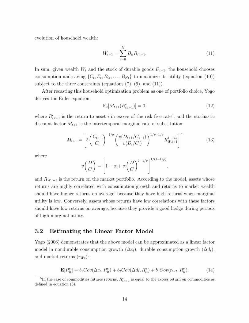
3.2 Estimating the Linear Factor Model

Yogo (2006) demonstrates that the above model can be approximated as a linear factor

model in nondurable consumption growth (∆ct), durable consumption growth (∆dt),

and market returns (rWt):

E[Reit] = b1Cov(∆ct, R

eit) + b2Cov(∆dt, R

eit) + b3Cov(rWt, R

eit). (14)

5In the case of commodities futures returns, Rei,t+1 is equal to the excess return on commodities asdefined in equation (3).

14

The risk prices b are a function of the preference parameters in the model:

b =

b1b2b3

=

κ[1/σ + α(1/ρ− 1/σ)]

κα(1/σ − 1/ρ)

1− κ

. (15)

Furthermore, this model can be estimated using two-step GMM. Define the vector of

factors, ft = [∆ct,∆dt, rWt]′, and its expectation µf = E[ft]. We can estimate the

model using the moment function:

e(zt, θ) =

[Ret −Re

t (ft − µf )′b(ft − µf )

](16)

and weighting matrices:

W1 =

[kIN 0

0 Σ̂−1ff

]and W2 = S−1,

where k > 0 is a constant and Σ̂ff is a consistent estimator of Σff , the variance-

covariance matrix of ft.6

The two-step GMM is solved using constrained linear minimization. Following Yogo

(2006), I impose two constraints on the risk prices that arise from their relationships

with the preference parameters of the model. Using Equation 15, we have that σ =

(1−b3)/(b1+b2), γ = b1+b2+b3, and α = b2/[b1+b2+(b3−1)/ρ].7 The first constraint,

that b1 + b2 + b3 ≥ 0, ensures that the risk aversion (γ) is nonnegative. The second

constraint, that b3 ≤ 0, ensures that the elasticity of intertemporal substitution (σ) is

nonnegative when b2 and b3 are nonnegative.8

The commodities returns in this and all further estimations of the linear factor model

are the excess returns as defined and constructed in Section 2 and as summarized in

Table A.2. The factors used in the estimation, which are described in detail in Appendix

6The initial weighting matrix W1 puts equal weight on the first N moments. The constant k =[det(Σ̂ii)]

1/N is inversely related to the variance-covariance matrix of the initial values for the firstN moments. See Yogo (2006), Appendix C and Cochrane (2005), Chapter 13 for discussions of themoment function and choices for weighting matrices.

7Because α and ρ cannot be separately identified, I follow Yogo (2006) and use ρ = 0.79.8While the results indicate that the parameters are rarely constrained in the final solutions, the

restrictions do sometimes impact the initial values for the parameters, which are calculated as theconstrained OLS estimates of the coefficients of the linear factor model in equation 14.

15

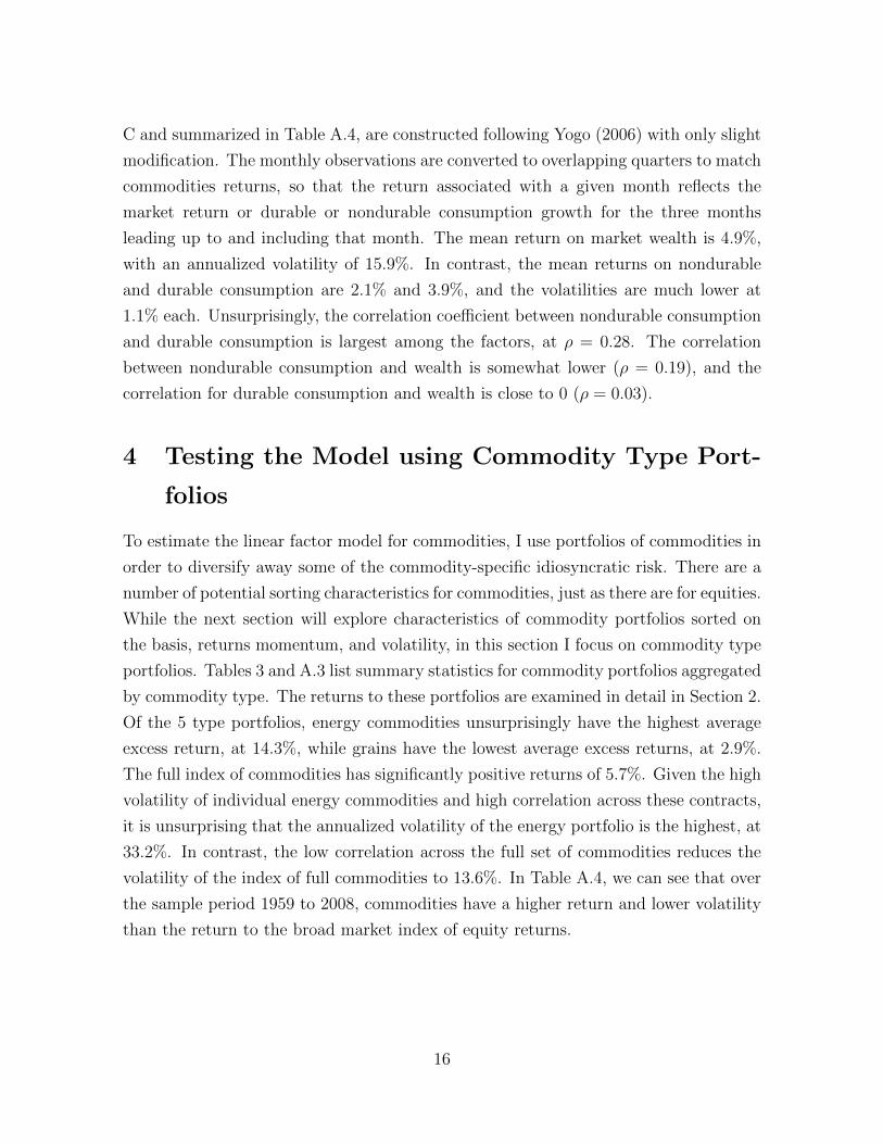
C and summarized in Table A.4, are constructed following Yogo (2006) with only slight

modification. The monthly observations are converted to overlapping quarters to match

commodities returns, so that the return associated with a given month reflects the

market return or durable or nondurable consumption growth for the three months

leading up to and including that month. The mean return on market wealth is 4.9%,

with an annualized volatility of 15.9%. In contrast, the mean returns on nondurable

and durable consumption are 2.1% and 3.9%, and the volatilities are much lower at

1.1% each. Unsurprisingly, the correlation coefficient between nondurable consumption

and durable consumption is largest among the factors, at ρ = 0.28. The correlation

between nondurable consumption and wealth is somewhat lower (ρ = 0.19), and the

correlation for durable consumption and wealth is close to 0 (ρ = 0.03).

4 Testing the Model using Commodity Type Port-

folios

To estimate the linear factor model for commodities, I use portfolios of commodities in

order to diversify away some of the commodity-specific idiosyncratic risk. There are a

number of potential sorting characteristics for commodities, just as there are for equities.

While the next section will explore characteristics of commodity portfolios sorted on

the basis, returns momentum, and volatility, in this section I focus on commodity type

portfolios. Tables 3 and A.3 list summary statistics for commodity portfolios aggregated

by commodity type. The returns to these portfolios are examined in detail in Section 2.

Of the 5 type portfolios, energy commodities unsurprisingly have the highest average

excess return, at 14.3%, while grains have the lowest average excess returns, at 2.9%.

The full index of commodities has significantly positive returns of 5.7%. Given the high

volatility of individual energy commodities and high correlation across these contracts,

it is unsurprising that the annualized volatility of the energy portfolio is the highest, at

33.2%. In contrast, the low correlation across the full set of commodities reduces the

volatility of the index of full commodities to 13.6%. In Table A.4, we can see that over

the sample period 1959 to 2008, commodities have a higher return and lower volatility

than the return to the broad market index of equity returns.

16

4.1 Estimating Risk Exposure using Time Series Regressions

Before turning to the results of the linear factor model, I investigate the time series

properties of commodities returns by examining the multiple betas for each portfolio.

These multiple betas are estimated using a separate time series regression for each

commodity portfolio.9 The regression coefficients measure the amount of risk each

commodity has relative to each factor within the three factor model:

Reit = βi0 + βic∆ct + βid∆dt + βiwrWt + εit (17)

The magnitude and significance of the multiple betas for each commodity can indicate

which factors are most important in the asset pricing of commodities futures. The

number of observations for each regression depends upon the data availability for that

particular type portfolio, and ranges from 307 for energy to 591 for grains. As before,

I adjust for serial correlation using Newey-West standard errors with 4 lags.

In Panel A of Table 3, we can see the first indication that durable consumption

growth is an important factor for commodities returns. For the index of all commodities,

we have a negative βc, and positive values for βd and βw. Of these, only βd is statistically

significant. The results for the five type portfolios also point to the importance of

durable consumption growth, as the estimate of βd is significant for the softs, metal,

and animal portfolios. Point estimates for βd are generally the largest in magnitude

as well, ranging from 2.09 for softs to 4.80 for metals. The only other statistically

significant factor beta is the market wealth beta for the metal portfolio (βw = 0.30).

However, there is no discernible pattern in market wealth risk, as the βw estimate is

negative for energy and grains portfolios and positive for softs, animals, and metals.

Finally, the results for the five type portfolios indicate that nondurable consumption

risk also differs quite a bit across commodity type, as the multiple beta for nondurable

consumption ranges from -5.86 for energy to 0.14 for animals.

9Though these multiple betas can also be estimated using the GMM estimation of the linear factormodel, the GMM estimates are affected by the choice of test assets used in the cross section and theprecision with which the GMM is able to estimate the population means of the factor returns. In orderto examine factor multiple betas which are free of these complicating factors, in this section I presentthe results from time series regressions instead.

17

4.2 Evidence and Evaluation for the Broader Cross Section

While examining the individual assets’ multiple betas helps us understand the amount

of risk exposure each asset has relative to the factors included, the linear factor model

allows us to determine how well these risk amounts and the estimated risk prices can

predict the average excess returns. In other words, the linear factor model allows us to

test the prediction that assets with higher betas and higher amounts of risk will have

higher excess returns.

In order to test whether this model can predict the returns of commodity portfolios,

I estimate the linear factor model using a broad cross section of potential assets in which

an individual may choose to invest. In addition to the 6 commodity portfolios, each

cross section may also include 6 Fama-French equity portfolios sorted on size and book-

to-market value, 5 equity portfolios sorted on industry characteristics, 6 bond portfolios,

3 indexes of international equities, and 6 foreign currency portfolios. A description of

portfolio construction and summary statistics for these assets can be found in Appendix

D.

GMM estimation requires that all included test assets have data availability over

the entire sample period chosen. Therefore, a cross section that includes the energy

portfolio must be limited to the sample period June 1983 to December 2008, which

leaves over two decades of data on most other commodities unused. In order to make

maximum use of the data available, I therefore estimate the model on a long sample

that covers March 1965 (when the animal portfolio begins) to December 2008 and a

short sample that covers January 1984 to December 2007, when data on the energy

portfolio, currency portfolios, and international equities are available. For the long

sample, the set of test assets includes all test assets for which the data is available for

the entire sample period: the grains, softs, animal, and metals portfolios, the 6 Fama-

French portfolios, the 5 industry-sorted equity portfolios, and the 6 bond portfolios.

For the short sample, I add to these the energy portfolio, the 3 international indexes

and the 6 currency portfolios.

The cross sectional results of the model, which can be found in Table 5, demonstrate

that the model describes the data well. The first estimation with the long sample gives

positive significant risk prices for durable and nondurable consumption growth, but a

negative risk price for market wealth. The high R2 (0.88) and low mean absolute error

(0.87 percentage points) are based on first-stage estimates for the 21 test assets, and

are visible in Figure 3(a), which graphs the actual returns to each test asset against

18

the predicted return. Furthermore, the J-test of overidentifying restrictions does not

reject the model (p = 0.98). For the short sample, the estimated risk prices for durable

consumption growth and market wealth are positive and significant, while the risk

price for nondurable consumption growth is negative and significant. The J-test does

not reject this model either (p = 1.00), and the R2 is an even higher 0.93. Figure 3(b)

graphs the actual and predicted returns for the short sample estimation.

According to the theory, these estimated risk prices can be used to calculate the

values of the preference parameters of the model. For the long sample, the risk prices

imply an elasticity of intertemporal substitution (σ) of 0.01, a coefficient of risk aversion

(γ) of 167.68, and a weight on durables (α) of 0.35. In the short sample, the estimate

for the elasticity of intertemporal substitution is similarly low (0.01), while the estimate

for the weight on durables is higher than for the long sample (1.52). Additionally, in

the short sample, the estimate for the coefficient of risk aversion is lower than for the

long sample, but still high (48.96). Yogo (2006) explains that the high coefficient of

risk aversion is an expression of the equity premium puzzle, which is driven by the low

volatility of nondurable and durable consumption relative to asset returns.

These results indicate that the consumption-based asset pricing model including

durable and nondurable consumption growth can predict returns to commodity type

portfolios and a broad cross section of assets. This result is at odds with earlier pa-

pers on commodities, which found that asset pricing models were not able to explain

commodities returns. However, it is consistent with conventional wisdom in the fi-

nance literature that while factor models might perform poorly when trying to explain

differences among individual assets, they are generally more successful at explaining

differences in returns across broad classes of assets. By grouping commodities into

portfolios based on type and then including these assets with many assets of diverse

origin, I am able to estimate a consumption-based multi-factor asset pricing model that

successfully predicts commodities returns.

Furthermore, these results indicate that durable consumption growth is an impor-

tant factor in the pricing of commodity portfolios. In time series regressions, coefficient

on the durable goods factor has the largest magnitude and most significance for com-

modity portfolios, indicating a strong correlation between commodities returns and

durable consumption growth. In the cross section, while theory would predict all risk

prices to be positive, the risk price on durable goods is the only consistently positive

significant one. This positive risk price is consistent with the theory that durables con-

sumption growth is an important factor in explaining the cross section of asset returns,

19

because it indicates that assets with higher durables risk have higher returns. While

the high returns to commodities and low correlation with nondurable consumption and

equity returns was previously puzzling, these results demonstrate that the high returns

to commodities can be explained by their high durables risk.

5 Characteristics driving commodities returns

5.1 Theory, Motivation, Construction

Given the success of the model in predicting commodities returns for portfolios based on

type, I further investigate which characteristics of commodities may be driving these

returns and risk amounts. There is a long history in finance of sorting equities into

portfolios according to characteristics that can predict returns, including size, book-

to-market value, and industry type, as in the Fama-French test assets used above.

Sorting assets into portfolios allows us to study the relationship between the underlying

sorting characteristic and asset returns by eliminating the other idiosyncratic drivers of

returns that can be diversified within each portfolio. For example, equity portfolios that

are sorted on size should contain equities with similar distributions of book-to-market

ratios. Comparing these size portfolios, and especially the spread between the extreme

portfolios, allows us to focus on the risk-return tradeoff of the size characteristic. These

ideas have also been applied by Lustig and Verdelhan (2007), who explain the returns

to investing in currency futures by sorting currencies into portfolios based on interest

rate differentials.

To identify potential sorting characteristics for commodities, I draw on a broad set

of theories on commodities returns, backwardation, and the storage model. In partic-

ular, this work is motivated by Gorton et al. (2007), who examine the empirical link

between inventories and the risk premium. They demonstrate patterns of returns to

portfolios of commodities sorted on inventories and priced-based signals of inventories,

such as the futures basis, spot return momentum, and excess return momentum. How-

ever, they stop short of testing the relationship between these predictors of returns and

conventional asset pricing models. In this paper, I focus on spot price volatility, the

basis, and excess return momentum as sorting characteristics, to see whether commod-

ity portfolios formed on these characteristics have returns that are predictable using

standard asset pricing models.

20

The first characteristic I use for sorting is the spot price volatility. If we view the

return to buying a futures contract as a reward for taking on the risk associated with

future spot price volatility, then we should expect returns to increase in periods of high

volatility and high risk. Furthermore, if past volatility is a predictor of future volatility,

when we sort on past volatility, we should see an increase in excess returns for the high

volatility portfolios. If spot price volatility also covaries predictably with the factors in

the consumption-based model, then we would find predictable patterns in the returns

to volatility-sorted portfolios. To measure recent volatility, I calculate for the end of

each month the three month coefficient of variation, which equals the variance of the

daily spot prices over the previous three months divided by the mean of these daily spot

prices. Finally, I sort commodities each month into five portfolios using the demeaned

value of recent spot price volatility.10

Given the focus on the basis as a predictor of spot returns in the Fama (1984)

regression (equation (6)), the basis is a natural choice for the second sorting character-

istic. More recently, Hong and Yogo (2010) and Gorton et al. (2007) have studied the

basis as one of the determinants of commodity returns and note that excess returns are

generally higher when the basis is low. They argue that a low basis is often a signal

of low inventories, which cause spot prices to rise more than futures prices. Since low

inventories can result in higher spot price risk, they also require higher excess returns.

By sorting commodities into portfolios using the basis, I measure the relationship be-

tween the basis and futures returns in a cross sectional, rather than time series, setting.

I construct the set of basis-sorted commodity portfolios by sorting commodities each

month using the demeaned monthly basis for each commodity.

The final sorting characteristic is returns momentum. In addition to being an im-

portant predictor of returns for equities, Gorton et al. (2007) point out that past returns

are likely indicative of unanticipated shocks to supply or demand. Since these shocks

may have lasting effects on prices and inventories, it is reasonable to think that past

returns, to the extent that they carry information about the state of inventories, will

be a good predictor of future returns. Indeed, Hong and Yogo (2010) and Gorton et al.

(2007) find high momentum commodities have higher returns. To capture the informa-

tion reflected in the history of excess returns, I construct a set of five portfolios sorted

on the demeaned value of the average of the previous twelve months of excess returns.

10Further details on portfolio construction can be found in Appendix B.

21

In addition to the five portfolios in each of the above sets, I add a sixth portfolio to

each set to measure the returns to a trading strategy that takes advantage of the spread

in returns across the extreme portfolios. For the basis sorted portfolios, this means going

long in the low basis portfolio and short in the high basis portfolio. For the momentum

and volatility sorted portfolios, it means going long in the high momentum/volatility

portfolio and short in the low momentum/volatility portfolio.

5.2 Summary Statistics and Time Series Properties of Com-

modity Portfolios

We can learn about the returns to these sorting characteristics by examining both the

average excess returns and the pattern of betas across the five portfolios. The trends

described in this section are visually represented by Figures 4(a)-4(c), which graph

the returns and time series betas for each portfolio. As shown in Figure 4(a), the

volatility-sorted portfolios indicate the patterns expected, with returns that increase

monotonically from the low volatility portfolio to the high volatility portfolio. The

high volatility portfolio has statistically significant returns of 24.7%, while the high-

minus-low portfolio generates a positive return of 26.8% and a Sharpe ratio of 0.80.

Looking at the pattern of betas across the 5 sorted portfolios in Panel B of Table 3

and Figure 4(a), it is clear that higher returns are consistent with higher durables risk,

as the positive, statistically significant values for βd increase with excess returns and

momentum. In other words, the returns to the high momentum portfolio covary more

strongly with durable consumption growth than the returns to the low momentum

portfolio. In contrast, the βw generally decrease with momentum, indicating that the

low momentum portfolio returns covary more strongly with returns to market wealth

than the high momentum portfolio returns. While none of the βw on the individual

portfolios is significant, the return to the high-minus-low portfolio, which measures the

spread in the returns to the momentum-sorted portfolios, is negative. Finally, the table

and figure show that βc does not vary consistently with the basis or returns.11

11Since nondurable and durable consumption are positively correlated, the multiple betas presentedhere could be quite different from simple betas calculated from univariate time series regressions.Simple betas are provided for in Table A.8 for comparison. While market and durables betas retainsimilar magnitudes and qualitative patterns, many nondurables betas are in fact positive in a univariatesetting where the durables factor is not included in the regression. However, since the nondurablesbetas still do not demonstrate a pattern of increasing with average returns across sorted portfolios,they remain unable to explain the cross section of commodities returns.

22

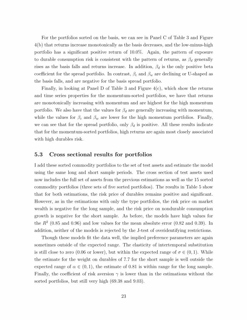
For the portfolios sorted on the basis, we can see in Panel C of Table 3 and Figure

4(b) that returns increase monotonically as the basis decreases, and the low-minus-high

portfolio has a significant positive return of 10.0%. Again, the pattern of exposure

to durable consumption risk is consistent with the pattern of returns, as βd generally

rises as the basis falls and returns increase. In addition, βd is the only positive beta

coefficient for the spread portfolio. In contrast, βc and βw are declining or U-shaped as

the basis falls, and are negative for the basis spread portfolio.

Finally, in looking at Panel D of Table 3 and Figure 4(c), which show the returns

and time series properties for the momentum-sorted portfolios, we have that returns

are monotonically increasing with momentum and are highest for the high momentum

portfolio. We also have that the values for βd are generally increasing with momentum,

while the values for βc and βw are lower for the high momentum portfolios. Finally,

we can see that for the spread portfolio, only βd is positive. All these results indicate

that for the momentum-sorted portfolios, high returns are again most closely associated

with high durables risk.

5.3 Cross sectional results for portfolios

I add these sorted commodity portfolios to the set of test assets and estimate the model

using the same long and short sample periods. The cross section of test assets used

now includes the full set of assets from the previous estimations as well as the 15 sorted

commodity portfolios (three sets of five sorted portfolios). The results in Table 5 show

that for both estimations, the risk price of durables remains positive and significant.

However, as in the estimations with only the type portfolios, the risk price on market

wealth is negative for the long sample, and the risk price on nondurable consumption

growth is negative for the short sample. As before, the models have high values for

the R2 (0.85 and 0.96) and low values for the mean absolute error (0.82 and 0.39). In

addition, neither of the models is rejected by the J-test of overidentifying restrictions.

Though these models fit the data well, the implied preference parameters are again

sometimes outside of the expected range. The elasticity of intertemporal substitution

is still close to zero (0.06 or lower), but within the expected range of σ ∈ (0, 1). While

the estimate for the weight on durables of 7.7 for the short sample is well outside the

expected range of α ∈ (0, 1), the estimate of 0.81 is within range for the long sample.

Finally, the coefficient of risk aversion γ is lower than in the estimations without the

sorted portfolios, but still very high (69.38 and 9.03).

23

A summary of these results is best represented by Figures 3(c) and 3(d), which plot

the realized average excess returns against the predicted average excess returns. While

the momentum and basis-sorted portfolios have returns that range from 1% to 12%

per annum, the realized returns for the volatility-sorted portfolios have a much larger

range, from -2% to 25%. Figure 3(c) illustrates that the model is able to accurately

predict this range of returns. Finally, Figure 3(d) demonstrates that the model also fits

well when using a short sample period.

6 Nested Special Cases and other Benchmark Mod-

els

The three factor model presented in Section 3 nests a number of well-known special

cases. In this section I present results for these linear factor models, each of which uses

only a subset of the three factors included in the main model and imposes corresponding

restrictions on the preference parameters of the model. I also present results for the

Fama-French three factor model as an additional benchmark. The results demonstrate

that durable consumption growth is an important factor in explaining the cross section

of asset returns.

Secondly, I present two robustness checks for the GMM estimations above. First,

in order to examine whether the risk prices change over time, I provide GMM esti-

mation using the same cross section of test assets over different sample periods. The

results indicate that while estimates of risk prices are not stable over time, the risk

price for durable consumption is the only one that is positive and significant in every

sample period. Finally, because consumption data may not be well-measured at the

monthly level, I present results using only nonoverlapping quarters. While data using

nonoverlapping quarters has the benefit of a lower autocorrelation across consecutive

observations, it also has the drawback of having a smaller number of observations in

the time series, which restricts further the number of test assets which may be included

in a sample of a given length. Even so, the results are consistent with those estimated

using overlapping quarterly data.

24

6.1 Nested Special Cases

The full three factor model presented in Section 3 nests a number of well-known asset

pricing models as special cases. Using the short cross section with sorted portfolios

(column 4 of Table 4), I present results for linear factor models which use one or two of

the three factors of the full model. The columns of Table 6 correspond to the following

special cases:

1. CAPM: The standard CAPM uses only market wealth as a factor. Preference

parameters are restricted such that b3 = γ, b1 = b2 = 0, σ = ρ, and σ →∞.

2. CCAPM: The consumption CAPM uses only nondurable consumption as a factor,

and restricts preference parameters to b1 = γ, b2 = b3 = 0, σ = 1/γ = ρ and α = 0.

3. DCAPM: The durable CAPM uses only durable consumption as a factor. Pref-

erence parameter restrictions are the same as those in the CCAPM, as this

model simply substitutes durable consumption growth for nondurable consump-

tion growth: b2 = γ, b1 = b3 = 0, σ = 1/γ = ρ and α = 1.

4. EZ-CCAPM: The Epstein-Zin CAPM uses nondurable consumption and market

wealth as factors. Once again defining κ ≡ (1 − γ)/(1 − 1σ), we have preference

parameter restrictions: b1 = κ/σ, σ = ρ, b2 = 0, and b3 = 1− κ.

5. CD-CAPM: The nonseparable expected utility model uses nondurable and durable

consumption as factors. Preference parameters are restricted such that σ = 1/γ,

b1 = γ + α(1/ρ− γ), b2 = α(γ − 1/ρ), b3 = 0, and ρ = 0.79 by assumption.

6. EZ-DCAPM: Results for the full three factor model are reproduced for ease of

reference. As before, b1 = κ[1/σ+α(1/ρ−1/σ)], b2 = κα(1/σ−1/ρ), b3 = 1−κσ,

and ρ = 0.79 by assumption.

Comparing the first three models which have one factor each, it is clear that the

durable CAPM has the most explanatory power. The durable CAPM is the only model

for which the R2 is higher than 0.9 and the mean absolute error is below 1%. The

relatively strong fit of the model can be seen in Figure 5(c) as compared to Figures

5(a) and 5(b). In fact, the durable CAPM with only one factor has a higher R2 and

lower mean absolute error than the EZ-CCAPM, which has nondurable consumption

and market wealth as factors.

25

Comparing the results of the DCAPM to the results in columns 5 and 6 of Table

6, we can see that the R2 falls from 0.985 to 0.977 and then rises to 0.991. Similarly,

the mean absolute error rises when the nondurable consumption factor is added, going

from 0.457 to 0.584, but then falls to 0.391 when the market returns factor is added.

When using a linear factor model to explain returns to a cross section of international

assets and commodity portfolios, these results indicate that once durable consumption

is included as a factor, the addition of nondurable consumption does not add much ex-

planatory power to the model. Additionally, these results indicate that adding durable

consumption to a model with only nondurable consumption and market returns as

factors does improve explanatory power.

One final important benchmark model is the three factor Fama-French model, which

uses market returns as well as the size and value spread portfolios as factors. The SMB

factor measures the spread in returns between equities with small and large market

capitalizations, while the HML factor measures the spread in returns between equities

with high and low book-to-market values. The results in column 7 of Table 6 show that

the three factor Fama-French model performs better than many of the nested mod-

els discussed above. However, it is outperformed by all models which include durable

consumption growth as a factor, including the one-factor DCAPM, the two-factor CD-

CAPM, and the full three-factor model with nondurable consumption, durable con-

sumption, and market returns.

6.2 Risk Prices over Time

The cross sectional results in Table 5 show large differences in risk prices across the

four specifications. These differences could be due to either the inclusion of different

assets in each cross section or the different sample periods used for each estimation. In

order to further investigate whether the risk prices have changed over time, I estimate

the model using an early and late sample period for the same cross section.

Table 7 provides results using the set of assets that are available in the early sam-

ple period, which includes the domestic equities and bonds, and all the commodity

portfolios except for energy (column 3 of Table 4). In addition to the early and late

samples, the results for the full sample period are reproduced for ease of reference. The

estimated risk price for each factor differs across sample periods. While the changes in

parameter estimates may reflect changes in the actual risk price over time, they could

also reflect the difficulty in estimating the parameters using limited sample periods. In

26

fact, the full sample risk prices are not always an intermediate value between the two

short sample estimates. However, despite the inconsistency across sample periods, it

is important to note that the durables risk price is the only risk price that remains

significant and positive for all sample periods.

6.3 Nonoverlapping Quarters

In Table 8, I present results using nonoverlapping quarterly data. These cross sectional

estimates use the same long and short sample periods as in the estimates using over-

lapping quarterly data. However, while the cross section of test assets in the two long

sample estimations remain the same as before, the short sample estimations must be

adjusted. As noted by Burnside (2007), GMM estimation requires the number of test

assets to be relatively small compared to the sample length. When using nonoverlap-

ping quarters, the sample length for the short sample period is small (T=96), so the

cross section must be limited.

One way to limit the number of test assets is to use only the index of all commodities

rather than the 5 type portfolios. Additionally, I replace the 5 sorted portfolios for

each of the sorting variables with the spread portfolios (High-Minus-Low Momentum

and Volatility, and Low-Minus-High Basis). To demonstrate that the fit of the model is

robust to various choices in the cross section of test assets, I estimate the model on two

very different cross sections. The first is a set of primarily domestic test assets, which

adds to the 4 commodity portfolios the 6 Fama-French equity portfolios, 5 industry-

sorted equity portfolios, 6 bond portfolios, one index of international equities, and

one currency portfolio that measures the spread between high and low interest rate

currencies. The second cross section is an internationally focused one, and includes the

4 commodity portfolios as well as the Small-Minus-Big equity portfolio, the High-Minus-

Low equity portfolio, the 6 bond portfolios, 3 international indexes, and 7 currency

portfolios.

For these 4 estimations, the results are little changed from before. While the risk

price on nondurables and market wealth change signs for the long samples as compared

to the previous set of estimations, the risk price on durables remains positive and

significant for all 4 estimations. In addition, the R2 remains high (0.92 or higher),

and the mean absolute error remains roughly the same as before. The parameter

values remain of a similar magnitude: relatively small for the elasticity of intertemporal

substitution (hitting the lower bound of 0 for the short domestic sample), the coefficient

27

of risk aversion remains high, and the weight on durables is higher than the expected

range of α ∈ (0, 1). Finally, while the p-value for the J-test of overidentifying restrictions

falls to below 0.05 for the long sample with sorted commodity portfolios, the J-test fails

to reject the model for the other three estimations.

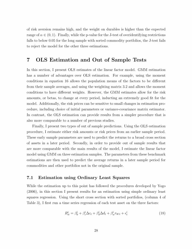
7 OLS Estimation and Out of Sample Tests

In this section, I present OLS estimates of the linear factor model. GMM estimation

has a number of advantages over OLS estimation. For example, using the moment

conditions in equation 16 allows the population means of the factors to be different

from their sample averages, and using the weighting matrix 3.2 and allows the moment

conditions to have different weights. However, the GMM estimates allow for the risk

amounts, or betas, to change at every period, inducting an extremely good fit for the

model. Additionally, the risk prices can be sensitive to small changes in estimation pro-

cedure, including choice of initial parameters or variance-covariance matrix estimator.

In contrast, the OLS estimation can provide results from a simpler procedure that is

also more comparable to a number of previous studies.

Finally, I present two types of out of sample predictions. Using the OLS estimation

procedure, I estimate either risk amounts or risk prices from an earlier sample period.

These early sample parameters are used to predict the returns to a broad cross section

of assets in a later period. Secondly, in order to provide out of sample results that

are more comparable with the main results of the model, I estimate the linear factor

model using GMM on three estimation samples. The parameters from these benchmark

estimations are then used to predict the average returns in a later sample period for

commodities and other portfolios not in the original sample.

7.1 Estimation using Ordinary Least Squares

While the estimation up to this point has followed the procedures developed by Yogo

(2006), in this section I present results for an estimation using simple ordinary least

squares regression. Using the short cross section with sorted portfolios, (column 4 of

Table 3), I first run a time series regression of each test asset on the three factors:

Reit = βi0 + βic∆ct + βid∆dt + βiwrWt + εit (18)

28

Next, I estimate the risk prices using a single cross sectional regression of the average

return to each test asset on the estimated time series betas:

Reit = λcβ̂

ic + λdβ̂

id + λwβ̂

iw + εi. (19)

Column 1 of Table 9 presents the results of this cross sectional regression.12 While

the coefficient on durables risk is positive, it is not statistically distinguishable from

zero. Meanwhile, the risk price of market returns is positive and significant, and the

risk price on nondurable growth is negative and significant. The R-squared for this

regression is 0.22, and mean absolute error indicates that the cross sectional regression

predicts the average returns to commodity portfolios about as well as the returns to

all the test assets, on average. Figure 6(a) graphs the actual returns to each test asset

against the predicted return for the OLS estimation.

Given that the risk prices change depending on the cross section of test assets, I

also estimate the cross sectional regression using only the 20 commodity portfolios. In

the results reported in column 2, we can see that the risk price on durables is the only

positive one, though it is still not significant. Additionally, the R-squared is even higher,

at 0.51. These results provide additional evidence that while a number of assets have

returns that increase with market risk, the average returns to commodity portfolios

instead increase with durable consumption risk.

Finally, I provide two more OLS estimations for comparison. Column 3 provides

results for the cross section of 25 Fama-French equity portfolios sorted on size and

book-to-market value. For this estimation, the risk price of market returns is the only

positive one. However, the R-squared is negative. These results, along with Figure 6(c),

provide evidence that OLS estimation of the linear factor model does not perform well

even for the benchmark test assets. In comparison with these results, the OLS results

for commodities look even stronger. Column 4 and Figure 6(d) provide results for the

EZ-CCAPM, which is the nested model with only nondurable consumption and market

returns as factors. The poor fit of this model provide further evidence that even in an

OLS estimation, the durables factor helps explain the returns to commodity portfolios.

12Since the regressors here are betas, rather than covariances, the risk prices (λ) are not necessarilyequal to the risk prices (b) in the previous cross sectional analyses. Consequently, they also do nothave the same relationship with the preference parameters of the model in Section 3.

29

7.2 Out of Sample Tests using OLS

Another way to check the robustness of the results is to examine how the model per-

forms out of sample. In this section, I perform three of out of sample tests using OLS

regressions. For each test, either risk amounts or risk prices are estimated using an early

sample period. These early sample parameters are used to predict the cross section of

average returns in a later period. These out of sample estimations are performed using

the short cross section with sorted portfolios (column 4 of Table 4).

In the first out of sample test, I use the OLS cross sectional regression to test

whether betas from an earlier period are able to predict average returns in a later

period. I first estimate the time series betas from equation 18 for each portfolio in the

cross section by using the first half of the available sample period (January 1984 to

December 1995). Next, I regress the average return to each portfolio over the second

half of the sample period (January 1996 to December 2007) on these early sample betas

in the cross sectional regression (equation 19).

For both the full cross section (column 3) and the subset of commodity portfolios

(column 4), the results in Table 10 indicate that the risk price for durable consumption

is significant and positive. As compared to the in-sample OLS estimation (reproduced

in column 1), the full cross section has slightly higher mean absolute error and a lower

R-squared. In contrast, the subset of just the commodity portfolios has a slightly

lower mean absolute error and a higher R-squared than in the in-sample OLS estima-

tion (column 2). Figures 7(a) and 7(b) demonstrate that the fit of the model for the

out of sample estimation are similar to the corresponding in-sample OLS estimation,

represented by Figures 6(a) and 6(b).

For the second out of sample test, I estimate the risk prices using the first half of

the available sample period (January 1984 to December 1995). This requires using the

same time series betas from the early sample period as in the previous estimation. I

estimate the early sample risk prices by regressing the average return to each portfolio

over the first half of the period on these early sample betas, using the cross sectional

regression (equation 19). These risk prices are reported in columns 5 and 6 of Table

10. Finally, I estimate the time series betas using the second half of the sample period

(January 1996 to December 2007), and use the early sample risk prices and the late

sample betas to predict the average returns to each portfolio. The measures of fit in

columns 5 and 6 of Table 10 are calculated using these predicted average returns and

the actual average returns over the late sample period.

30

The results indicate that the risk prices calculated in the early sample do not help

predict the average returns in the late sample period. The mean absolute error and

R-squared values in columns 5 and 6 of Table 10 are quite poor compared to previous

in-sample and out of sample estimations. These results are consistent with previous

evidence that risk prices seem to change over time.

7.3 Out of Sample Tests using GMM

While the OLS out of sample tests allow evaluation of the model using either risk

prices or risk amounts estimated from an early sample, the results are comparable only

to the in-sample OLS estimates and not to the in-sample GMM estimations. In this

section, I provide out of sample estimations that are more directly comparable to the

main results, which are estimated by GMM. Here, I use various samples to estimate the

linear factor model (equation 14) by GMM, using the moments in equation 16. I use

the estimated risk prices and factor population means to predict the average returns in

a later sample period for commodities and other portfolios not in the original sample.

Finally, I examine how well these predicted returns fit the actual cross section of returns

using various measures of fit.

In the first set of out of sample tests, I use GMM to estimate the risk prices for

market returns, nondurable and durable consumption. Using an early sample period

of January 1959 to December 1983, I estimate the model on the 25 benchmark Fama-

French equity portfolios sorted on size and book-to-market values. The results of this

estimation are reported in column 1 of Table 11. Using the parameter estimates for

risk prices (b) and factor means (µ), I calculate the predicted values and residuals for a

broad cross section of test assets. In particular, I use the short cross section with sorted

portfolios (column 4 of Table 4), except that I omit the 6 Fama-French portfolios since

they are similar to the 25 benchmark portfolios used in the estimation of the parameters.

The results in Panel A of Table 12 indicate that the fit of the model is not as strong

when the parameters are estimated out of sample. While the J-test does not reject

the hypothesis that the pricing errors are jointly zero for the full cross section of out

of sample assets in column 1, this hypothesis is rejected for the subset that includes

only the commodity portfolios (column 2). The R-squared and the mean absolute error

indicate that the out of sample predictions have much worse fit than the in-sample

predictions, as reported in Table 5. Figures 8(a) and 8(b) graph the actual returns

to each test asset against the predicted return from the GMM estimation. They show

31

that this out of sample estimation generally over-predicts the returns to the test assets,

especially for assets with a high actual return.

These results are consistent with previous evidence that risk prices change depending

on the sample period and cross section of test assets included. A second out of sample

test estimates the risk prices using the same set of 25 Fama-French portfolios but

extends the sample period to December 2008. The risk prices, reported in column 2

of Table 11, are somewhat changed. Panel B of Table 12 shows that these risk prices

are better able to predict average returns. While the R-squared is better for the full

sample, it is worse for the set of commodity portfolios. However, the J-test does not

reject the model for either set of portfolios. Figures 8(c) and 8(d) provide graphical

illustrations.

The third out of sample test estimates the risk prices using the set of assets that are

available in the early sample period, which includes the domestic equities and bonds,

and all the commodity portfolios except for energy (column 3 of Table 4). Using these

risk prices, reported in column 3 of Table 11, the out of sample tests have a much higher

R-squared and much lower mean absolute error. These results, graphically represented

by Figures 8(e) and 8(f), are comparable to the in-sample estimates in Table 5. However,

the J-test rejects the hypothesis that the pricing errors are jointly zero for the full set

of test assets and for the subset of commodity portfolios.

8 Business Cycle Properties

The strong fit of the consumption-based multi-factor model indicates that the returns

to commodities and other assets can be explained by their covariance with the three

factors that affect investors’ marginal utility: nondurable and durable consumption

growth, and returns to market wealth. In particular, the results indicate that durable

consumption growth is a key factor in explaining the returns to commodities. While the

Yogo (2006) model of household optimization explains why assets with durables risk

require high returns, it leaves open the question of why commodities have high durables

risk. In this section, I examine the business cycle properties of commodities returns

in order to further explore the link between commodities and durable consumption

growth.

First, returning to the model presented in Section 3, we can see why assets with

high durables risk require high returns. When utility is not additively separable in

32

nondurable and durable consumption, marginal utility has an extra multiplicative term,

v(D/C)κ(1/ρ−1/σ). When ρ > σ and κ > 0 (σ < 1 and γ > 1), marginal utility of

nondurable consumption rises when durable consumption falls. The results support

this theory, as the parameters fall well within these restrictions. The high durables risk

of commodities means that commodities have low returns when durable consumption

growth is low. This is precisely when marginal utility of consumption is high. Therefore,

returns to these risky commodities must be high on average for households to invest in

them.

Next, in order to explain the high durables risk of commodities, I turn to examining

their business cycle properties. Gorton and Rouwenhorst (2006) note that commodities

returns behave differently than stock and bond returns over the business cycle. Using

the dates determined by the NBER Business Cycle Dating Committee, they classify

each month as being part of one of the four phases of the business cycle, splitting each

expansion and recession into “early” and “late” periods by simply dividing the full

period in half. For each series (stocks, bonds, and an index of commodities returns),

they take the average return over all months in each phase to determine the peaks and

troughs. They find that while stocks peak in early expansion, commodities returns peak

in late expansion. In addition, stock returns trough in early recession while commodities

returns trough in late recession. These results show that while stocks and commodities

both have higher returns in expansions than in recessions, splitting the business cycle

into four phases can better illuminate the low correlation between commodities and

equities.

Following their work, I perform a similar analysis on the five commodities type port-

folios and the consumption-based risk factors of durable and nondurable consumption

growth. The results in Table 13 indicate that returns to each commodity type portfo-

lio and the returns to the index of all commodities follow a pattern similar to that of

durable consumption growth. In addition, nondurable consumption growth follows the

same pattern as market returns. While nondurables and market returns peak in early

expansion, durables and commodity portfolios returns peak in late expansion. While

nondurables and market returns trough in early recession, durables and commodity

portfolios trough in late recession.

Though these patterns are not evidence of a causal link between durable consump-

tion growth and commodities returns, they do indicate a timing pattern that may

explain the strong correlation between durables and commodities. Commodity portfo-

lios deliver high returns when durable consumption growth is high, which means they

33

have weak hedging properties. According to the model, commodities therefore must

have high returns on average. Furthermore, this analysis provides corroborating ev-

idence that commodities returns have low risk exposure to nondurable consumption

growth and market returns, which may further explain why previous attempts at using

the CAPM or consumption-based CAPM were unsuccessful.

This similar timing of durable consumption growth and commodities returns may

be caused by a basic link between the use of commodities in the production of durable

goods. Another possibility is that these two series have similar behavior over the busi-

ness cycle because each has a cycle that slightly lags that of nondurable consumption,

but for different reasons. For instance, the returns to commodities may be driven by

the level of inventories of commodities. If the timing of this inventory is like that of the

general inventory cycle, which lags the usual business cycle indicators, then commodi-

ties returns will also lag the usual business cycle. If durable consumption growth also

lags the usual business cycle for unrelated reasons, we will see high covariance between

commodities returns and durable consumption growth. A covariance between com-

modities and durables consumption growth that is driven by similar timing rather than

a causal link is still consistent with the model. According to the model, the investor

cares about getting high returns when marginal utility is high. Commodity portfolios

which deliver high returns when durable consumption growth is high must have high

returns on average, because they have weak hedging properties.

9 Conclusion

Using a consumption-based multi-factor asset pricing model, I have demonstrated that

the high returns to commodities can be explained by their high correlation with durable

goods consumption growth. Previous papers have been unable to explain the high

returns to commodities and have also been unable to reconcile their high returns with

their low correlation with nondurable consumption and market returns. In this paper,

I have shown that adding durable consumption growth as a factor can resolve both

issues. Because commodities returns are highly correlated with durable consumption

growth, in the context of the model, the high average returns to commodities provide

compensation for the high durables risk a commodities investor assumes. By including

durable goods as a factor in the model, I am able to measure the strong correlation

34

between commodities and durables and accurately predict the high average returns to

commodities.

In time series regressions, the correlation between commodities returns and durables

results in significant positive coefficients on the durable consumption growth factor.

Grouping commodities by type allows me to diversify some idiosyncratic elements of the

individual commodities futures markets, and better analyze the underlying patterns.

Furthermore, when commodities are sorted into portfolios using known correlates of

commodities returns, including the basis, momentum, and volatility, the coefficient on

durable goods increases with sorted portfolio returns. These results indicate that the

importance of durable goods as a factor is consistent with existing explanations of

commodities returns.

In the cross section, after including durable goods in the household investors’ utility

function, I use the linear factor model to predict average returns to each asset in the

cross section. The results indicate that the three factor model is very successful at

predicting the range of returns across a variety of test assets. Furthermore, the GMM

estimates for the preference parameters of the model indicate that durable goods play

an important role in the utility of household investors. Additionally, by testing the same

cross section of test assets on the nested special cases of the model, I am also able to

demonstrate that inclusion of durable consumption growth as a factor is important for

explaining the cross section of returns, relative to the nondurable consumption growth

and market returns factors.

Finally, by examining commodities returns over the business cycle, I demonstrate

that returns to each commodity type portfolio and the returns to the index of all

commodities follow a pattern similar to that of durables consumption growth. While

nondurables and market returns peak in early expansion, durables and commodity port-

folios returns peak in late expansion. In addition, while nondurables and market returns

trough in early recession, durables and commodity portfolios trough in late recession.

These results begin to indicate one way in which durables growth and commodities re-

turns may be linked, and may suggest a causal explanation for the importance of durable

consumption growth as a factor for explaining the high returns to commodities.

35

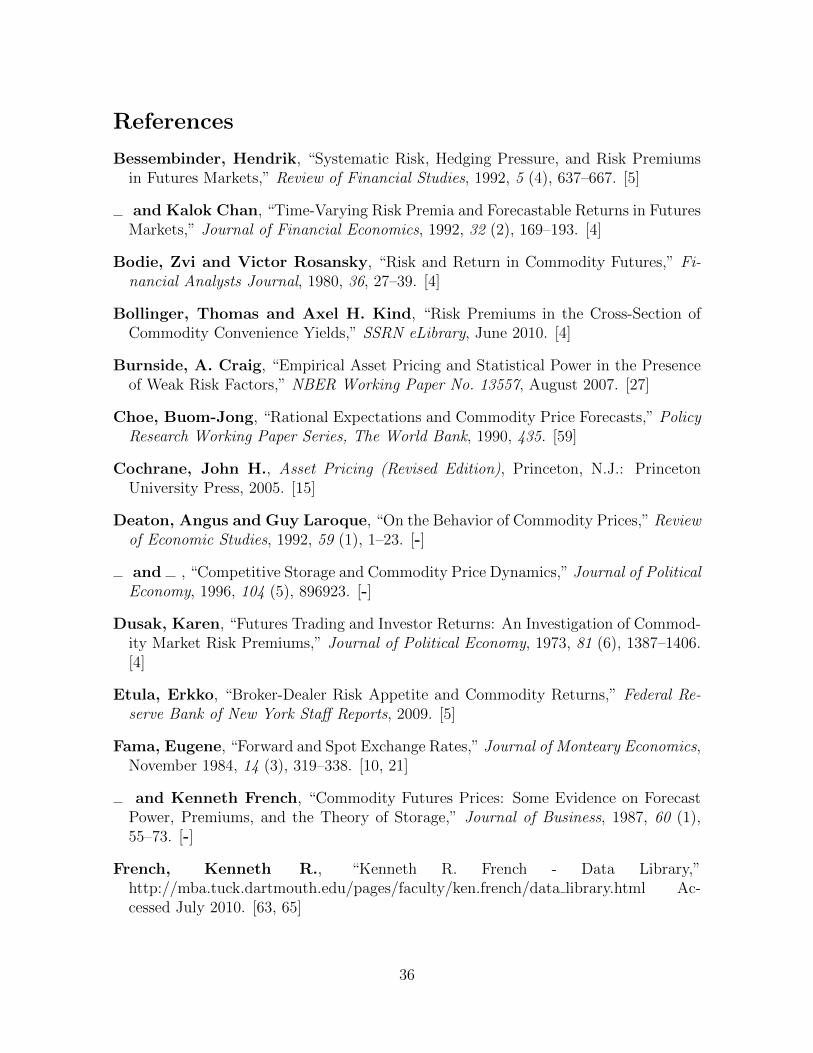
References

Bessembinder, Hendrik, “Systematic Risk, Hedging Pressure, and Risk Premiumsin Futures Markets,” Review of Financial Studies, 1992, 5 (4), 637–667. [5]

and Kalok Chan, “Time-Varying Risk Premia and Forecastable Returns in FuturesMarkets,” Journal of Financial Economics, 1992, 32 (2), 169–193. [4]

Bodie, Zvi and Victor Rosansky, “Risk and Return in Commodity Futures,” Fi-nancial Analysts Journal, 1980, 36, 27–39. [4]

Bollinger, Thomas and Axel H. Kind, “Risk Premiums in the Cross-Section ofCommodity Convenience Yields,” SSRN eLibrary, June 2010. [4]

Burnside, A. Craig, “Empirical Asset Pricing and Statistical Power in the Presenceof Weak Risk Factors,” NBER Working Paper No. 13557, August 2007. [27]

Choe, Buom-Jong, “Rational Expectations and Commodity Price Forecasts,” PolicyResearch Working Paper Series, The World Bank, 1990, 435. [59]

Cochrane, John H., Asset Pricing (Revised Edition), Princeton, N.J.: PrincetonUniversity Press, 2005. [15]

Deaton, Angus and Guy Laroque, “On the Behavior of Commodity Prices,” Reviewof Economic Studies, 1992, 59 (1), 1–23. [-]

and , “Competitive Storage and Commodity Price Dynamics,” Journal of PoliticalEconomy, 1996, 104 (5), 896923. [-]

Dusak, Karen, “Futures Trading and Investor Returns: An Investigation of Commod-ity Market Risk Premiums,” Journal of Political Economy, 1973, 81 (6), 1387–1406.[4]

Etula, Erkko, “Broker-Dealer Risk Appetite and Commodity Returns,” Federal Re-serve Bank of New York Staff Reports, 2009. [5]

Fama, Eugene, “Forward and Spot Exchange Rates,” Journal of Monteary Economics,November 1984, 14 (3), 319–338. [10, 21]

and Kenneth French, “Commodity Futures Prices: Some Evidence on ForecastPower, Premiums, and the Theory of Storage,” Journal of Business, 1987, 60 (1),55–73. [-]

French, Kenneth R., “Kenneth R. French - Data Library,”http://mba.tuck.dartmouth.edu/pages/faculty/ken.french/data library.html Ac-cessed July 2010. [63, 65]

36

Gilmore, Stephen and Fumio Hayashi, “Emerging Market Currency Excess Re-turns,” NBER Working Paper No. 14258, December 2008. [10]

Gorton, Gary and K. Geert Rouwenhorst, “Facts and Fantasies About Com-modity Futures,” Financial Analysts Journal, 2006, 62 (2), 47–68. [3, 4, 6, 7, 33,58]

, Fumio Hayashi, and K. Geert Rouwenhourst, “The Fundamentals of Com-modities Futures Returns,” NBER Working Paper No. 13249, July 2007. [3, 7, 20,21, 58]

Hong, Harrison G. and Motohiro Yogo, “Commodity Market Interest and AssetReturn Predictability,” SSRN eLibrary, 2010. [3, 5, 6, 7, 21, 58]

Jagannathan, Ravi, “An Investigation of Commodity Futures Prices Using theConsumption-Based Intertemporal Capital Asset Pricing Model,” Journal of Fi-nance, 1985, 40 (1), 175–191. [5]

Lustig, Hanno and Hanno Verdelhan, “The Cross Section of Foreign CurrencyRisk Premia and Consumption Growth Risk,” American Economic Review, March2007, 91 (1), 89–117. [2, 20]

, Nikolai Roussanov, and Hanno Verdelhan, “Common Risk Factors in Cur-rency Markets,” NBER Working Paper No. 14082, 2008. [61, 66]

, , and , “Monthly Currency Excess Returns,” URL:http://web.mit.edu/adrienv/www/Data.html Accessed June 2010. [65]

Rogers, Jim, “Breakfast of Champions?,” URL:http://www.jimrogers.com/content/indexofarticles.html July 2002. [4, 6]

Yogo, Motohiro, “A Consumption-Based Explanation of Expected Stock Returns,”Journal of Finance, April 2006, 61 (2), 539–580. [2, 6, 13, 14, 15, 16, 19, 28, 32, 42,63, 64]

37

Table 1: Test for Unconditional Excess Returns

Commodity Mean Ann. Sharpe Start(% p.a.) Volatility Ratio p-value T Date

Grains 2.93 21.8 0.14 0.31 591 Oct ’59Corn -2.09 24.3 -0.09 0.52 591 Sept ’59Soybeans 5.24 27.8 0.19 0.15 591 Sept ’59Soybean Oil 7.80* 32.3 0.24 0.08 591 Sept ’59Soybean Meal 8.68** 31.1 0.28 0.03 590 Dec ’59Wheat -0.12 25.4 -0.01 0.97 591 Sept ’59Oats -1.22 28.2 -0.04 0.74 590 Dec ’59Rough Rice -0.36 34.6 -0.01 0.96 266 Nov ’86

Softs 3.50 17.9 0.20 0.15 583 June ’60Cocoa 3.91 32.8 0.12 0.38 587 Mar ’60Cotton 1.51 24.6 0.06 0.66 583 Jul ’60Sugar 7.36 48.7 0.15 0.29 572 Jul ’61Orange Juice 4.44 33.1 0.13 0.35 500 May ’67Lumber -1.53 28.4 -0.05 0.72 467 Mar ’70Coffee 7.04 41.4 0.17 0.29 431 Mar ’73

Metal 6.27* 24.2 0.26 0.07 542 Nov ’63Silver 1.70 33.3 0.05 0.72 542 Aug ’63Gold -0.88 19.9 -0.04 0.79 406 Jan ’75Copper 11.52*** 31.3 0.37 0.01 591 Oct ’59Aluminum 4.03 28.6 0.14 0.33 487 Aug ’99Platinum 8.33 38.1 0.22 0.19 377 Jul ’68Palladium 2.21 20.1 0.11 0.72 113 Mar ’77Zinc -2.14 29.7 -0.07 0.74 251 Feb ’88Nickel 12.88 45.4 0.28 0.17 250 Mar ’88Tin 3.00 24.3 0.12 0.60 232 Sept ’89Lead 7.50 31.3 0.24 0.31 210 Jul ’91

Animal 6.16** 18.9 0.33 0.02 526 Mar ’65Pork Bellies 3.12 32.7 0.10 0.47 539 Feb ’64Lean Hogs 7.08** 24.8 0.29 0.04 510 Jul ’66Live Cattle 6.01*** 16.9 0.36 0.01 526 Apr ’65Feeder Cattle 3.72 16.4 0.23 0.14 441 Mar ’72Milk 10.17 32.2 0.32 0.24 149 Apr ’96Butter 9.66 34.4 0.28 0.30 139 Feb ’97

Energy 14.32** 33.2 0.43 0.02 307 June ’83Heating Oil 13.56** 35.7 0.38 0.02 359 Feb ’79Crude Oil 14.12** 35.2 0.40 0.03 307 June ’83Gasoline 20.50*** 35.7 0.57 0.00 262 Feb ’85Propane 22.94*** 49.1 0.47 0.01 254 Dec ’87Natural Gas 8.09 49.0 0.17 0.43 222 June ’90Coal 5.61 35.6 0.16 0.68 87 Sept ’01

All Commodities 5.69*** 13.6 0.42 0.00 591 Oct ’59

Notes: ∗p < 0.10, ∗∗p < 0.05, and ∗∗∗p < 0.01. Excess returns are calculated as(St − Ft−3,t)/Ft−3,t. Volatilities, standard errors, and p-values are calculated usingNewey-West standard errors with 4 lags.

38

Table 2: Test for Conditional Excess Returns

Commodity Mean Coefficients Joint test p-values(% p.a.) T α β H0 : α = 0 & β = 1

GrainsCorn -2.09 590 -0.003 0.891 0.660Soybeans 5.24 590 0.013 0.975 0.308Soybean Oil 7.80* 590 0.018* 0.250*** 0.003***Soybean Meal 8.68** 587 0.021** 0.903 0.107Wheat -0.12 590 0.001 0.864 0.614Oats -1.22 587 0.001 0.710** 0.120Rough Rice -0.36 264 -0.014 1.518*** 0.009***

SoftsCocoa 3.91 584 0.016 0.335** 0.054*Cotton 1.51 580 0.004 0.930 0.677Sugar 7.36 569 0.023 0.645 0.278Orange Juice 4.44 498 0.012 0.663 0.199Lumber -1.53 464 0.002 0.695*** 0.033**Coffee 7.04 428 0.019 0.464** 0.041**

MetalSilver 1.70 542 0.015 0.469 0.341Gold -0.88 406 0.015 0.037 0.579Copper 11.52*** 589 0.020** 0.162*** 0.000***Aluminum 4.03 484 0.018* -0.142** 0.058*Platinum 8.33 376 0.028* -0.018 0.083*Palladium 2.21 111 0.013 -0.569 0.598Zinc -2.14 251 0.002 0.696 0.505Nickel 12.88 250 0.041* 3.201*** 0.000***Tin 3.00 232 0.011 -0.154** 0.078*Lead 7.50 210 0.022 0.101* 0.118

AnimalPork Bellies 3.12 536 0.007 1.118 0.463Lean Hogs 7.08** 507 0.016* 0.914 0.053*Live Cattle 6.01*** 523 0.013** 0.770** 0.000***Feeder Cattle 3.72 438 0.009 0.970 0.331Milk 10.17 147 0.020 0.835 0.213Butter 9.66 136 0.020 0.909 0.706

EnergyHeating Oil 13.56** 357 0.030** 0.788 0.009***Crude Oil 14.12** 306 0.035* 1.036 0.079*Gasoline 20.50*** 261 0.050*** 1.047 0.005***Propane 22.94*** 251 0.064*** 1.260 0.023**Natural Gas 8.09 222 0.024 0.846 0.326Coal 5.61 86 0.014 1.113 0.798

Notes: Table reports results for the Fama Regression: SpotReturnt+3 =α + β(Basist) + εt+3. Stars on the point estimates of α and β indicate significancefor the hypotheses H0 : α = 0 and H0 : β = 1, respectively. The final column reportsthe p-value for the test of the joint hypothesis H0 : α = 0 & β = 1. ∗p < 0.10,∗∗p < 0.05, and ∗∗∗p < 0.01. Standard errors are calculated using Newey-Weststandard errors with 4 lags.

39

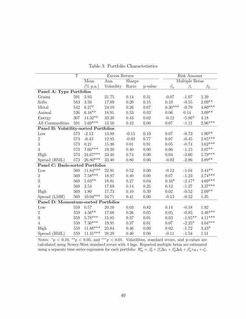
Table 3: Portfolio Characteristics

T Excess Return Risk AmountMean Ann. Sharpe Multiple Betas(% p.a.) Volatility Ratio p-value βw βc βd

Panel A: Type PortfoliosGrains 591 2.93 21.75 0.14 0.31 -0.07 -1.07 2.39Softs 583 3.50 17.89 0.20 0.15 0.10 -0.55 2.09**Metal 542 6.27* 24.19 0.26 0.07 0.30*** -0.79 4.80***Animal 526 6.16** 18.91 0.33 0.02 0.06 0.14 3.09**Energy 307 14.32** 33.20 0.43 0.02 -0.12 -5.86* 4.18All Commodities 591 5.69*** 13.58 0.42 0.00 0.07 -1.11 2.96***Panel B: Volatility-sorted PortfoliosLow 573 -2.13 13.88 -0.15 0.19 0.07 -0.73 1.90**2 573 -0.43 12.85 -0.03 0.77 0.07 -0.45 2.85***3 573 0.21 15.30 0.01 0.91 0.05 -0.74 3.62***4 573 7.66*** 19.20 0.40 0.00 0.06 -1.15 3.07**High 573 24.67*** 33.48 0.74 0.00 0.04 -3.60 5.79***Spread (HML) 573 26.80*** 33.40 0.80 0.00 -0.02 -2.86 3.89**Panel C: Basis-sorted PortfoliosLow 569 11.84*** 22.91 0.52 0.00 -0.12 -1.04 3.44**2 569 7.58*** 18.97 0.40 0.00 0.07 -1.23 3.74***3 569 5.03** 18.81 0.27 0.04 0.16* -2.17* 4.69***4 569 2.54 17.69 0.14 0.25 0.12 -1.27 3.37***High 569 1.80 17.73 0.10 0.39 0.02 -0.52 2.09**Spread (LMH) 569 10.04*** 24.71 0.41 0.00 -0.13 -0.52 1.35Panel D: Momentum-sorted PortfoliosLow 559 0.57 20.16 0.03 0.82 0.14 -0.18 1.922 559 4.56** 17.68 0.26 0.05 0.05 -0.85 3.46***3 559 5.78*** 15.85 0.37 0.01 0.03 -1.85** 4.11***4 559 7.30*** 19.91 0.37 0.01 0.07 -2.25* 4.04***High 559 11.88*** 25.84 0.46 0.00 0.02 -1.72 3.43*Spread (HML) 559 11.31*** 28.29 0.40 0.00 -0.11 -1.54 1.51

Notes: ∗p < 0.10, ∗∗p < 0.05, and ∗∗∗p < 0.01. Volatilities, standard errors, and p-values arecalculated using Newey-West standard errors with 4 lags. Reported multiple betas are estimatedusing a separate time series regression for each portfolio: Reit = βi0 +βic∆ct+βid∆dt+βiwrWt+ εit.

40

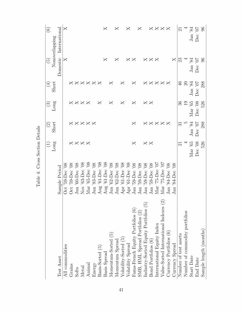
Tab

le4:

Cro

ssSec

tion

Det

ails

(1)

(2)

(3)

(4)

(5)

(6)

Lon

gShor

tL

ong

Shor

tN

onov

erla

ppin

gT

est

Ass

etSam

ple

Per

iod

Dom

esti

cIn

tern

atio

nal

All

com

modit

ies

Oct

’59-

Dec

’08

XX

Gra

ins

Oct

’59-

Dec

’08

XX

XX

Sof

tsJun

’60-

Dec

’08

XX

XX

Met

alN

ov’6

3-D

ec’0

8X

XX

XA

nim

alM

ar’6

5-D

ec’0

8X

XX

XE

ner

gyJun

’83-

Dec

’08

XX

Bas

is-S

orte

d(5

)A

ug

’61-

Dec

’08

XX

Bas

isSpre

adA

ug

’61-

Dec

’08

XX

Mom

entu

m-S

orte

d(5

)Jun

’62-

Dec

’08

XX

Mom

entu

mSpre

adJun

’62-

Dec

’08

XX

Vol

atilit

y-S

orte

d(5

)A

pr

’61-

Dec

’08

XX

Vol

atilit

ySpre

adA

pr

’61-

Dec

’08

XX

Fam

a-F

rench

Equit

yP

ortf

olio

s(6

)Jan

’59-

Dec

’08

XX

XX

XSM

B,

HM

LSpre

adP

ortf

olio

s(2

)Jan

’59-

Dec

’08

XIn

dust

ry-S

orte

dE

quit

yP

ortf

olio

s(5

)Jan

’59-

Dec

’08

XX

XX

XB

ond

Por

tfol

ios

(6)

Jan

’59-

Dec

’08

XX

XX

XX

Inte

rnat

ional

Equit

yIn

dex

Mar

’75-

Dec

’07

XX

XX

Val

ue-

Sor

ted

Inte

rnat

ional

Index

es(2

)M

ar’7

5-D

ec’0

7X

XX

Curr

ency

Por

tfol

ios

(6)

Jan

’84-

Dec

’08

XX

XC

urr

ency

Spre

adJan

’84-

Dec

’08

XN

um

ber

ofte

stas

sets

2131

3646

2321

Num

ber

ofco

mm

odit

yp

ortf

olio

s4

519

204

4Sta

rtD

ate

Mar

’65

Jan

’84

Mar

’65

Jan

’84

Jan

’84

Jan

’84

End

Dat

eD

ec’0

8D

ec’0

7D

ec’0

8D

ec’0

7D

ec’0

7D

ec’0

7Sam

ple

lengt

h(m

onth

s)52

628

852

628

896

96

41

Table 5: Cross-sectional results using two-step GMM

(1) (2) (3) (4)Type Portfolios Sorted Commodity Portfolios

Long Sample Short Sample Long Sample Short SampleMarket Returns -0.161 0.343*** -0.088 0.518***

(0.505) (0.107) (0.145) (0.129)Nondurable Growth 110.509*** -23.810*** 14.182** -51.962***

(23.149) (7.369) (6.199) (3.061)Durable Growth 57.327*** 72.432*** 55.291*** 60.470***

(17.695) (5.010) (5.756) (2.188)EIS (σ) 0.007** 0.014*** 0.016*** 0.057***

(0.003) (0.002) (0.002) (0.021)Risk Aversion (γ) 167.675*** 48.964*** 69.384*** 9.026***

(21.672) (4.953) (7.080) (2.870)Durables Weight (α) 0.345 1.516 0.812 7.656

(16.377) (9.053) (5.147) (18.970)Portfolios (N) 21 31 36 46Commodity portfolios 4 5 17 20Sample Length (T) 526 288 526 288R-squared 0.876 0.934 0.852 0.957MAE (%) 0.869 0.552 0.819 0.391Commodities MAE (%) 1.221 0.693 1.106 0.423J-test 7.932 3.081 18.446 17.746(p-value) (0.980) (1.000) (0.981) (1.000)

Notes: ∗p < 0.10, ∗∗p < 0.05, and ∗∗∗p < 0.01. Standard errors are calculated using the VARHACprocedure and automatic lag length selection using the AIC. R-squared values and mean absolutepricing errors (MAE) are calculated using first stage estimates for the N test assets. J-test iscalculated using second stage estimates for the N test assets. Because α and ρ cannot be separatelyidentified, I follow Yogo (2006) and use ρ = 0.79 for parameter calculations. Long sample coversMarch 1965 to December 2008. Short sample covers January 1984 to December 2007. See Table 4for list of test assets included in each cross sectional estimation.

42

Tab

le6:

Com

par

ison

wit

hB

ench

mar

kM

odel

s

(1)

(2)

(3)

(4)

(5)

(6)

(7)

Model

:C

AP

MC

CA

PM

DC

AP

ME

Z-C

CA

PM

CD

-CA

PM

EZ

-DC

AP

MF

ama-

Fre

nch

Fac

tors

:W

CD

W,

CC

,D

W,

C,

DW

,SM

B,H

ML

Mar

ket

Ret

urn

s3.

809*

**–

–-0

.533

–0.

518*

**5.

633*

**(0

.288

)–

–(0

.463

)–

(0.1

29)

(0.1

64)

Non

dura

ble

Gro

wth

–18

1.68

9***

–22

1.69

8***

-5.0

04*

-51.

962*

**SM

B:

1.99

5***

–(7

.871

)–

(9.3

90)

(2.8

54)

(3.0

61)

(0.1

65)

Dura

ble

Gro

wth

––

58.0

85**

*–

75.0

11**

*60

.470

***

HM

L:

0.81

5–

–(1

.370

)–

(2.1

70)

(2.1

88)

(0.1

56)

EIS

(σ)

∞0.

006*

**0.

017*

**0.

007*

**0.

014*

**0.

057*

**–

–(0

.000

)(0

.000

)(0

.002

)(0

.000

)(0

.021

)–

Ris

kA

vers

ion

(γ)

3.80

9***

181.

689*

**58

.085

***

221.

166*

**70

.006

***

9.02

6***

–(0

.288

)(7

.871

)(1

.370

)(9

.478

)(2

.349

)(2

.870

)–

Dura

ble

sW

eigh

t(α

)–

01

01.

091

7.65

6–

––

––

(2.8

81)

(18.

970)

–P

ortf

olio

s(N

)46

4646

4646

4646

Com

modit

yp

ortf

olio

s20

2020

2020

2020

Sam

ple

Len

gth

(T)

288

288

288

288

288

288

288

R-s

quar

ed0.

402

0.82

50.

985

0.87

90.

977

0.99

10.

915

MA

E(%

)2.

572

1.32

20.

457

1.28

90.

584

0.39

10.

984

Com

modit

ies

MA

E(%

)3.

511

1.80

10.

424

1.29

80.

523

0.42

30.

684

J-t

est

36.0

0454

.553

5.02

755

.955

5.61

417

.746

31.5

94(p

-val

ue)

(0.8

29)

(0.1

56)

(1.0

00)

(0.1

07)

(1.0

00)

(1.0

00)

(0.9

01)

Not

es:

∗ p<

0.10

,∗∗p<

0.05

,an

d∗∗

∗ p<

0.0

1.

Sam

ple

per

iod

isJanu

ary

1984

toD

ecem

ber

2007.

See

Tab

le4,

colu

mn

6fo

rli

stof

test

asse

tsin

clu

ded

inth

ecr

oss

sect

ion

.E

stim

atio

nan

dpre

fere

nce

para

met

erre

stri

ctio

ns

are

as

des

crib

edin

Sec

tion

6.1

:(1

)C

CA

PM

:b 1

=γ

,b 2

=b 3

=0,σ

=1/γ

=ρ

andα

=0.

(2)

DC

AP

M:b 2

=γ

,b 1

=b 3

=0,σ

=1/γ

=ρ

an

dα

=1.

(3)

CA

PM

:b 3

=γ

,b 1

=b 2

=0,σ

=ρ,

an

dσ→∞

.(4

)E

Z-C

CA

PM

:κ≡

(1−γ

)/(1−

1 σ),b 1

=κ/σ

,σ

=ρ,b 2

=0,

an

db 3

=1−κ

.(5

):C

D-C

AP

M:σ

=1/γ

,b 1

=γ

+α

(1/ρ−γ

),b 2

=α

(γ−

1/ρ),b 3

=0,

andρ

=0.

79.

(6)

EZ

-DC

AP

M:b 1

=κ

[1/σ

+α

(1/ρ−

1/σ

)],b 2

=κα

(1/σ−

1/ρ),b 3

=1−κσ

,an

dρ

=0.

79.

See

also

not

esto

Tab

le5.

43

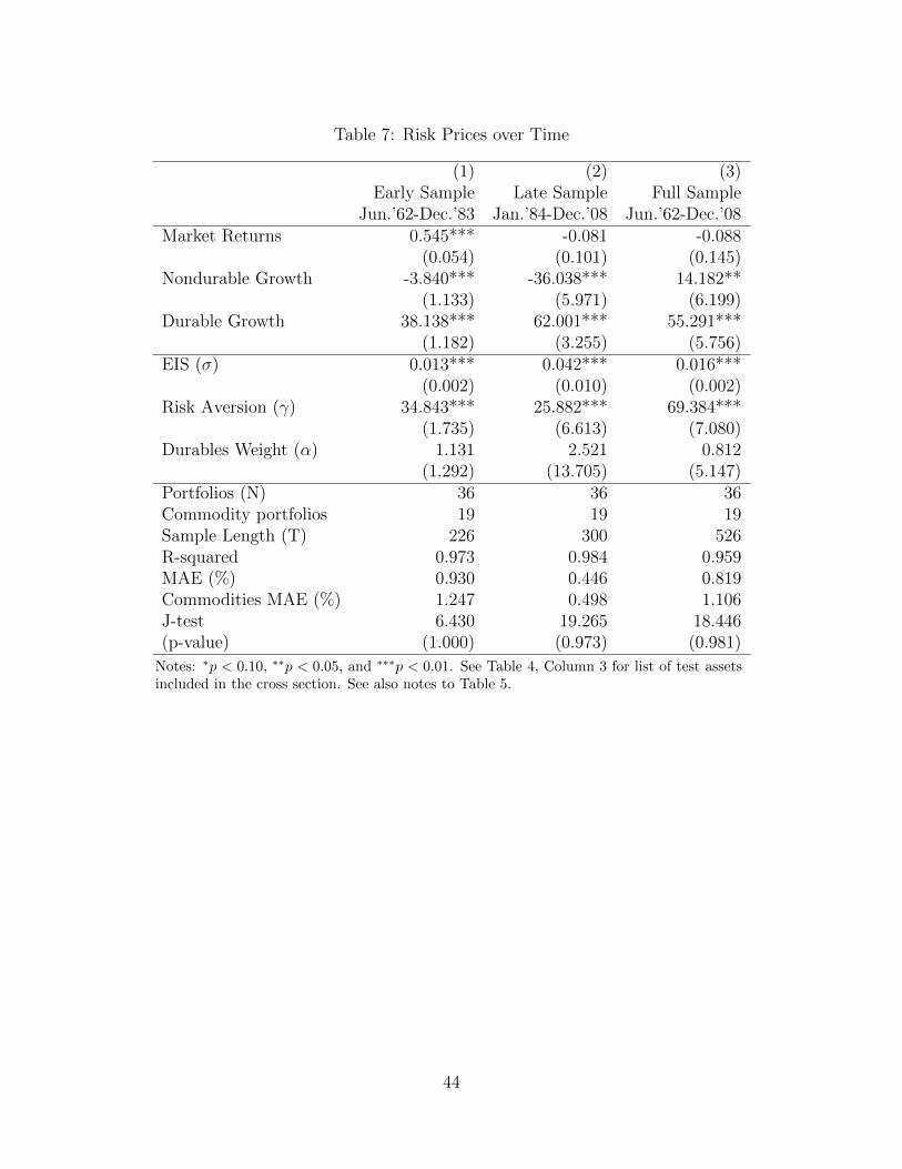
Table 7: Risk Prices over Time

(1) (2) (3)Early Sample Late Sample Full Sample

Jun.’62-Dec.’83 Jan.’84-Dec.’08 Jun.’62-Dec.’08Market Returns 0.545*** -0.081 -0.088

(0.054) (0.101) (0.145)Nondurable Growth -3.840*** -36.038*** 14.182**

(1.133) (5.971) (6.199)Durable Growth 38.138*** 62.001*** 55.291***

(1.182) (3.255) (5.756)EIS (σ) 0.013*** 0.042*** 0.016***

(0.002) (0.010) (0.002)Risk Aversion (γ) 34.843*** 25.882*** 69.384***

(1.735) (6.613) (7.080)Durables Weight (α) 1.131 2.521 0.812

(1.292) (13.705) (5.147)Portfolios (N) 36 36 36Commodity portfolios 19 19 19Sample Length (T) 226 300 526R-squared 0.973 0.984 0.959MAE (%) 0.930 0.446 0.819Commodities MAE (%) 1.247 0.498 1.106J-test 6.430 19.265 18.446(p-value) (1.000) (0.973) (0.981)

Notes: ∗p < 0.10, ∗∗p < 0.05, and ∗∗∗p < 0.01. See Table 4, Column 3 for list of test assetsincluded in the cross section. See also notes to Table 5.

44

Table 8: Results using nonoverlapping quarters

(1) (2) (3) (4)Type Portfolios Sorted Commodity Portfolios

Long Sample Long Sample Short Domestic Short InternationalMarket Returns 0.342 0.170 1.000*** 0.466

(0.323) (0.152) (0.168) (0.457)Nondurable Growth -58.875*** -51.363*** -44.116*** -84.887***

(11.763) (6.158) (6.204) (16.435)Durable Growth 107.448*** 59.302*** 86.956*** 114.277***

(14.430) (4.108) (4.242) (7.898)EIS (σ) 0.014** 0.105* 0.000 0.018

(0.006) (0.061) (0.004) (0.020)Risk Aversion (γ) 48.915*** 8.109* 43.840*** 29.856

(14.725) (4.459) (6.535) (19.699)Durables Weight (α) 2.251 8.609 2.030 3.980

(24.850) (29.455) (12.106) (71.298)Portfolios (N) 21 36 23 21Commodity portfolios 4 19 4 4Sample Length (T) 176 176 96 96R-squared 0.876 0.934 0.852 0.957MAE (%) 0.869 0.552 0.819 0.391Commodities MAE (%) 1.221 0.693 1.106 0.423J-test 7.932 3.081 18.446 17.746(p-value) (0.980) (1.000) (0.981) (1.000)

Notes: ∗p < 0.10, ∗∗p < 0.05, and ∗∗∗p < 0.01. Long sample covers March 1965 to December 2008.Short sample covers January 1984 to December 2007. See Table 4 for list of test assets included ineach cross sectional estimation. See also notes to Table 5.

45

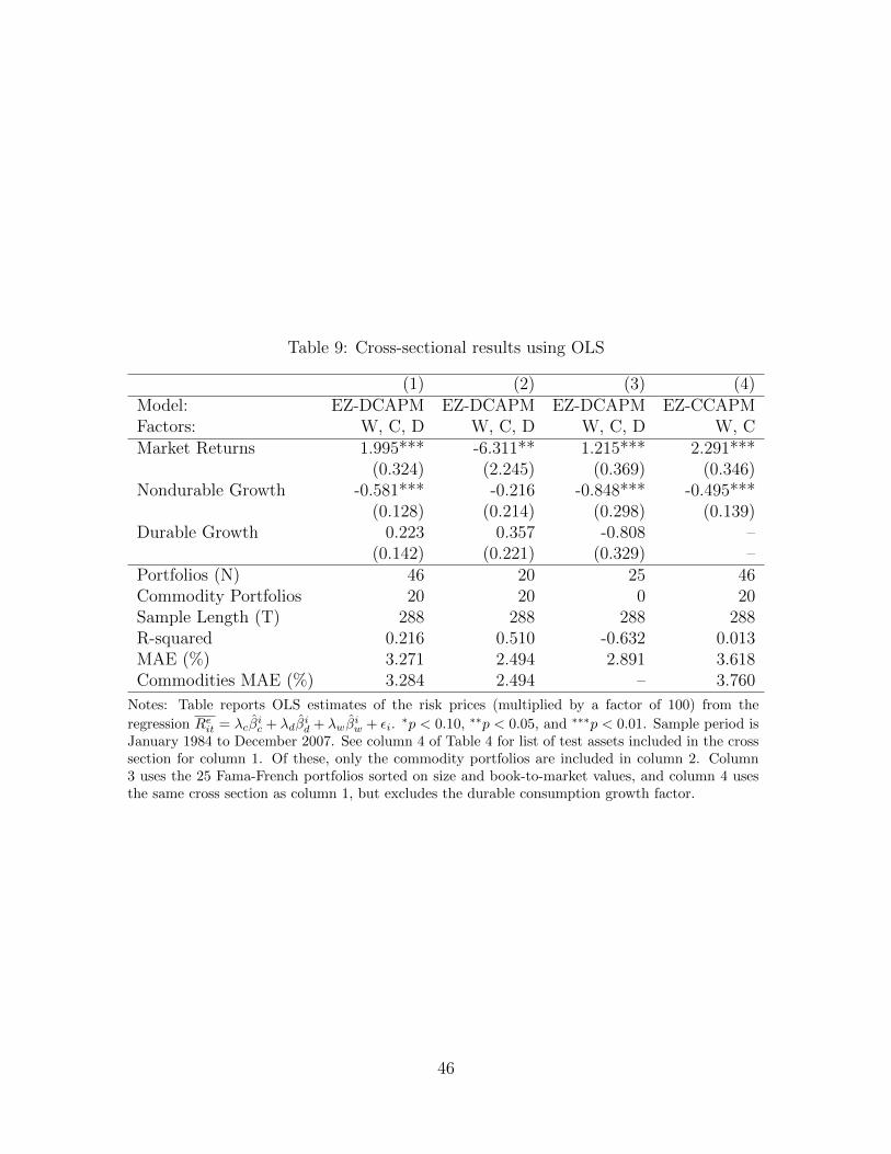
Table 9: Cross-sectional results using OLS

(1) (2) (3) (4)Model: EZ-DCAPM EZ-DCAPM EZ-DCAPM EZ-CCAPMFactors: W, C, D W, C, D W, C, D W, CMarket Returns 1.995*** -6.311** 1.215*** 2.291***

(0.324) (2.245) (0.369) (0.346)Nondurable Growth -0.581*** -0.216 -0.848*** -0.495***

(0.128) (0.214) (0.298) (0.139)Durable Growth 0.223 0.357 -0.808 –

(0.142) (0.221) (0.329) –Portfolios (N) 46 20 25 46Commodity Portfolios 20 20 0 20Sample Length (T) 288 288 288 288R-squared 0.216 0.510 -0.632 0.013MAE (%) 3.271 2.494 2.891 3.618Commodities MAE (%) 3.284 2.494 – 3.760

Notes: Table reports OLS estimates of the risk prices (multiplied by a factor of 100) from the

regression Reit = λcβ̂ic + λdβ̂

id + λwβ̂

iw + εi.

∗p < 0.10, ∗∗p < 0.05, and ∗∗∗p < 0.01. Sample period isJanuary 1984 to December 2007. See column 4 of Table 4 for list of test assets included in the crosssection for column 1. Of these, only the commodity portfolios are included in column 2. Column3 uses the 25 Fama-French portfolios sorted on size and book-to-market values, and column 4 usesthe same cross section as column 1, but excludes the durable consumption growth factor.

46

Tab

le10

:O

LS

Out

ofSam

ple

Est

imat

ion

(1)

(2)

(3)

(4)

(5)

(6)

Full

Sam

ple

Ear

lySam

ple

Bet

asE

arly

Sam

ple

Ris

kP

rice

sO

LS

Est

imat

ion

Lat

eSam

ple

Ris

kP

rice

sL

ate

Sam

ple

Bet

asA

llp

ortf

olio

sC

omm

odit

ies

All

por

tfol

ios

Com

modit

ies

All

por

tfol

ios

Com

modit

ies

Mar

ket

Ret

urn

s1.

995*

**-6

.311

**1.

921*

**-4

.505

***

2.36

0***

-2.7

44**

(0.3

24)

(2.2

45)

(0.3

75)

(1.0

26)

(0.3

24)

(2.2

45)

Non

dura

ble

Gro

wth

-0.5

81**

*-0

.216

-0.4

60**

*0.

019

-0.2

96**

*-0

.045

(0.1

28)

(0.2

14)

(0.1

02)

(0.0

94)

(0.1

28)

(0.2

14)

Dura

ble

Gro

wth

0.22

30.

357

0.25

0**

1.22

3***

0.27

10.

193

(0.1

42)

(0.2

21)

(0.1

10)

(0.2

11)

(0.1

42)

(0.2

21)

Por

tfol

ios

(N)

4620

4620

4620

Com

modit

yP

ortf

olio

s20

2020

2020

20Sam

ple

Len

gth

(T)

288

288

288

288

288

288

R-s

quar

ed0.

216

0.51

00.

014

0.75

0-1

.800

-2.1

80M

AE

(%)

3.27

12.

494

4.40

22.

348

6.75

59.

307

Com

modit

ies

MA

E(%

)3.

284

2.49

45.

373

2.34

89.

803

9.30

7

Not

es:

Tab

lere

por

tsO

LS

esti

mat

esof

the

risk

pri

ces

(mu

ltip

lied

by

afa

ctor

of

100)

from

the

regre

ssio

nRe it

=λcβ̂i c

+λdβ̂i d

+λwβ̂i w

+ε i

.∗ p<

0.10

,∗∗p<

0.05

,an

d∗∗

∗ p<

0.01

.S

eeco

lum

n4

of

Tab

le4

for

list

of

test

ass

ets

incl

ud

edin

the

cross

sect

ion

for

colu

mn

s1,

3,

an

d5.

Of

thes

e,on

lyth

eco

mm

od

ity

por

tfol

ios

are

incl

ud

edin

colu

mn

s2,

4,

an

d6.

Fu

llsa

mp

lep

erio

dis

Janu

ary

1984

toD

ecem

ber

2007,

earl

ysa

mp

leis

Jan

uar

y19

84to

Dec

emb

er19

95,

and

late

sam

ple

isJanu

ary

1996

toD

ecem

ber

2007.

Colu

mn

s1

an

d2

pro

vid

efu

llsa

mp

lees

tim

ate

s.C

olu

mn

s3

and

4re

gres

sla

tesa

mp

leav

erag

ere

turn

son

earl

ysa

mp

leti

me

seri

esb

etas.

Colu

mn

s5

and

6re

port

risk

pri

ces

esti

mate

du

sin

gea

rly

sam

ple

tim

ese

ries

bet

asan

dea

rly

sam

ple

aver

age

retu

rns.

Th

ese

earl

ysa

mp

leri

skp

rice

sare

use

dw

ith

late

sam

ple

tim

ese

ries

be-

tas

top

red

ict

aver

age

retu

rns.

Mea

sure

sof

fit

com

pare

thes

ep

red

icte

dre

turn

sw

ith

act

ualav

erage

retu

rns.

See

Sec

tion

7.2

for

furt

her

det

ail

s.

47

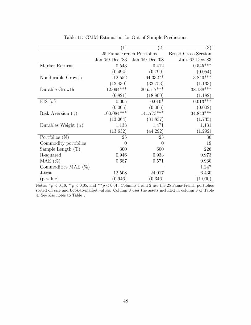
Table 11: GMM Estimation for Out of Sample Predictions

(1) (2) (3)25 Fama-French Portfolios Broad Cross Section

Jan.’59-Dec.’83 Jan.’59-Dec.’08 Jun.’62-Dec.’83Market Returns 0.543 -0.412 0.545***

(0.494) (0.790) (0.054)Nondurable Growth -12.552 -64.332** -3.840***

(12.430) (32.753) (1.133)Durable Growth 112.094*** 206.517*** 38.138***

(6.821) (18.800) (1.182)EIS (σ) 0.005 0.010* 0.013***

(0.005) (0.006) (0.002)Risk Aversion (γ) 100.084*** 141.773*** 34.843***

(13.064) (31.837) (1.735)Durables Weight (α) 1.133 1.471 1.131

(13.632) (44.292) (1.292)Portfolios (N) 25 25 36Commodity portfolios 0 0 19Sample Length (T) 300 600 226R-squared 0.946 0.933 0.973MAE (%) 0.687 0.571 0.930Commodities MAE (%) – – 1.247J-test 12.508 24.017 6.430(p-value) (0.946) (0.346) (1.000)

Notes: ∗p < 0.10, ∗∗p < 0.05, and ∗∗∗p < 0.01. Columns 1 and 2 use the 25 Fama-French portfoliossorted on size and book-to-market values. Column 3 uses the assets included in column 3 of Table4. See also notes to Table 5.

48

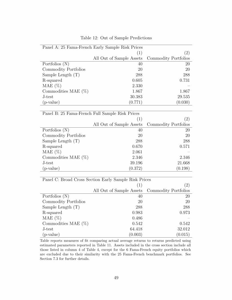
Table 12: Out of Sample Predictions

Panel A: 25 Fama-French Early Sample Risk Prices(1) (2)

All Out of Sample Assets Commodity PortfoliosPortfolios (N) 40 20Commodity Portfolios 20 20Sample Length (T) 288 288R-squared 0.605 0.731MAE (%) 2.330 –Commodities MAE (%) 1.867 1.867J-test 30.383 29.535(p-value) (0.771) (0.030)

Panel B: 25 Fama-French Full Sample Risk Prices(1) (2)

All Out of Sample Assets Commodity PortfoliosPortfolios (N) 40 20Commodity Portfolios 20 20Sample Length (T) 288 288R-squared 0.670 0.571MAE (%) 2.061 –Commodities MAE (%) 2.346 2.346J-test 39.196 21.668(p-value) (0.372) (0.198)

Panel C: Broad Cross Section Early Sample Risk Prices(1) (2)

All Out of Sample Assets Commodity PortfoliosPortfolios (N) 40 20Commodity Portfolios 20 20Sample Length (T) 288 288R-squared 0.983 0.973MAE (%) 0.486 –Commodities MAE (%) 0.542 0.542J-test 64.418 32.012(p-value) (0.003) (0.015)

Table reports measures of fit comparing actual average returns to returns predicted usingestimated parameters reported in Table 11. Assets included in the cross section include allthose listed in column 4 of Table 4, except for the 6 Fama-French equity portfolios whichare excluded due to their similarity with the 25 Fama-French benchmark portfolios. SeeSection 7.3 for further details.

49

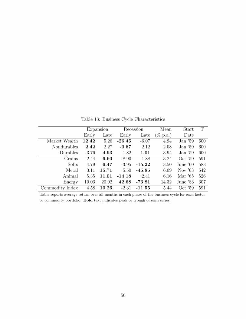
Table 13: Business Cycle Characteristics

Expansion Recession Mean Start TEarly Late Early Late (% p.a.) Date

Market Wealth 12.42 5.26 -26.45 -6.07 4.94 Jan ’59 600Nondurables 2.42 2.27 -0.67 2.12 2.08 Jan ’59 600

Durables 3.76 4.93 1.82 1.01 3.94 Jan ’59 600Grains 2.44 6.60 -8.90 1.88 3.24 Oct ’59 591

Softs 4.79 6.47 -3.95 -15.22 3.50 June ’60 583Metal 3.11 15.71 5.50 -45.85 6.09 Nov ’63 542

Animal 5.35 11.01 -14.18 2.41 6.16 Mar ’65 526Energy 10.03 20.02 42.68 -73.81 14.32 June ’83 307

Commodity Index 4.58 10.26 -2.31 -11.55 5.44 Oct ’59 591

Table reports average return over all months in each phase of the business cycle for each factor

or commodity portfolio. Bold text indicates peak or trough of each series.

50

Figure 1: Spot Price and Market Returns Indexes

Figure 2: Commodities Index and Factor Returns

(a) Commodities and Market Returns

(b) Nondurable and Durable Consumption Growth

51

Figure 3: GMM Cross Sectional Results

(a) Type Portfolios, Long Sample (b) Type Portfolios, Short Sample

(c) Sorted Portfolios, Long Sample (d) Sorted Portfolios, Short Sample

Notes: Each figure presents results for the corresponding column of Table 5. Figures graph therealized return to each portfolio against the predicted return according to two-step GMM estimation.See Table 4 for detailed list of test assets included in each cross section.

52

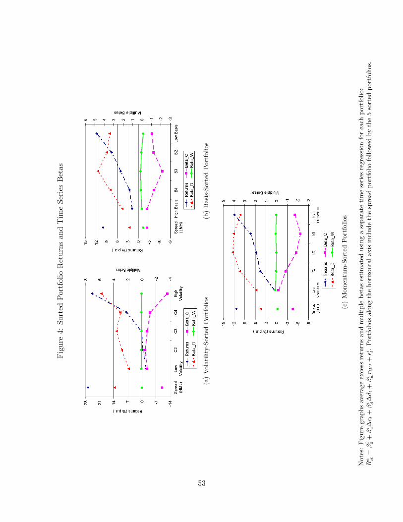
Fig

ure

4:Sor

ted

Por

tfol

ioR

eturn

san

dT

ime

Ser

ies

Bet

as

(a)

Vol

atil

ity-S

orte

dP

ort

foli

os

(b)

Basi

s-S

ort

edP

ort

foli

os

(c)

Mom

entu

m-S

ort

edP

ort

foli

os

Not

es:

Fig

ure

grap

hs

aver

age

exce

ssre

turn

san

dm

ult

iple

bet

as

esti

mate

du

sin

ga

sep

ara

teti

me

seri

esre

gre

ssio

nfo

rea

chp

ort

foli

o:

Re it

=βi 0

+βi c∆c t

+βi d∆dt

+βi wr W

t+εi t

.P

ortf

olios

alo

ng

the

hori

zonta

laxis

incl

ud

eth

esp

read

port

foli

ofo

llow

edby

the

5so

rted

port

foli

os.

53

Fig

ure

5:G

MM

Cro

ssSec

tion

alR

esult

sfo

rN

este

dSp

ecia

lC

ases

(a)

CA

PM

(W)

(b)

CC

AP

M(C

)(c

)D

CA

PM

(D)

(d)

EZ

-CC

AP

M(W

,C)

(e)

CD

-CA

PM

(C,D

)(f

)E

Z-D

CA

PM

(W,C

,D)

Not

es:

Eac

hfi

gure

pre

sents

resu

lts

for

the

corr

esp

on

din

gco

lum

nof

Tab

le6.

Fig

ure

sgra

ph

the

reali

zed

retu

rnto

each

port

foli

oagain

stth

ep

red

icte

dre

turn

acco

rdin

gto

two-

step

GM

Mes

tim

ati

on

of

the

spec

ified

mod

el.

54

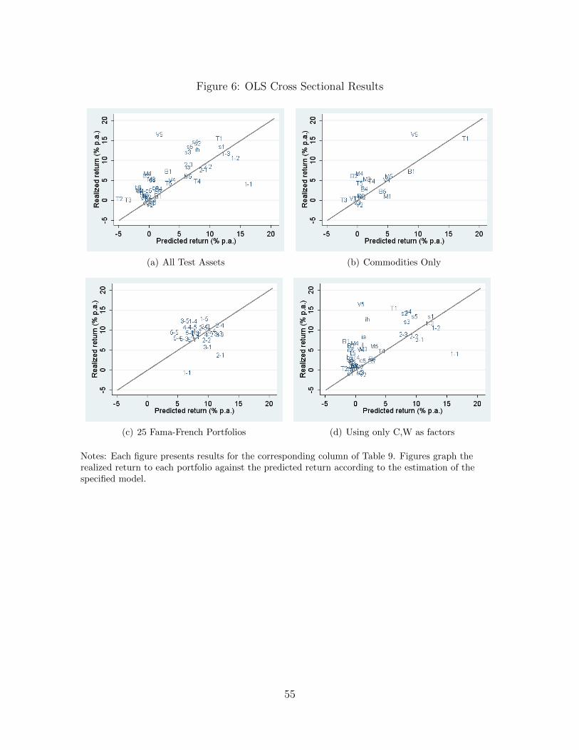
Figure 6: OLS Cross Sectional Results

(a) All Test Assets (b) Commodities Only

(c) 25 Fama-French Portfolios (d) Using only C,W as factors

Notes: Each figure presents results for the corresponding column of Table 9. Figures graph therealized return to each portfolio against the predicted return according to the estimation of thespecified model.

55

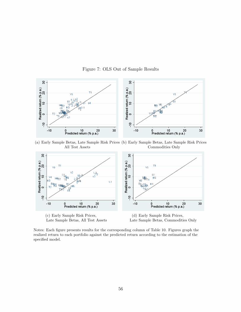
Figure 7: OLS Out of Sample Results

(a) Early Sample Betas, Late Sample Risk PricesAll Test Assets

(b) Early Sample Betas, Late Sample Risk PricesCommodities Only

(c) Early Sample Risk Prices,Late Sample Betas, All Test Assets

(d) Early Sample Risk Prices,Late Sample Betas, Commodities Only

Notes: Each figure presents results for the corresponding column of Table 10. Figures graph therealized return to each portfolio against the predicted return according to the estimation of thespecified model.

56

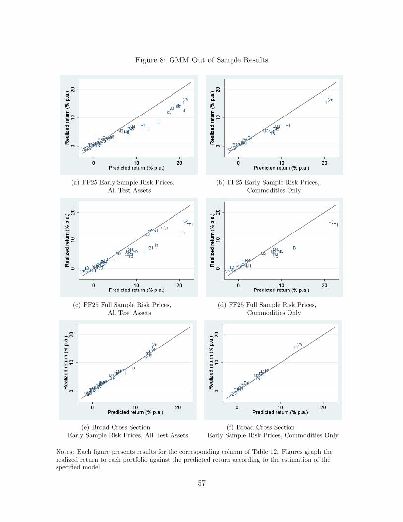
Figure 8: GMM Out of Sample Results

(a) FF25 Early Sample Risk Prices,All Test Assets

(b) FF25 Early Sample Risk Prices,Commodities Only

(c) FF25 Full Sample Risk Prices,All Test Assets

(d) FF25 Full Sample Risk Prices,Commodities Only

(e) Broad Cross SectionEarly Sample Risk Prices, All Test Assets

(f) Broad Cross SectionEarly Sample Risk Prices, Commodities Only

Notes: Each figure presents results for the corresponding column of Table 12. Figures graph therealized return to each portfolio against the predicted return according to the estimation of thespecified model.

57

Appendix A Commodities Data

This appendix provides summary statistics and data description for individual com-

modities and portfolios of commodities aggregated by type. Data comes from the Com-

modities Research Bureau (CRB), which provides daily prices on each contract from its

opening to its expiration. Because the CRB covers commodities futures markets that

are still in existence today, the set of included commodities is subject to survivor bias.

However, as noted by Gorton and Rouwenhorst (2006), commodities markets fail due

to lack of interest, unlike equities which usually fail due to poor performance and low

returns. Interest in a given commodities futures market is not necessarily correlated

with returns, since a negative return on a long futures position implies that the corre-

sponding short investor earns positive returns. In fact, while the futures markets for

corn and wheat have consistently yielded very low or even negative returns, they are

two of the oldest and most liquid markets.

Table A.1 lists individual futures contract coverage, including the exchange the

contract is traded on, the start and end date for contract availability, available contract

months, and number of monthly observations. To be consistent with related research,

this paper includes the set of CRB commodities with generally large production and

trading volumes (Gorton and Rouwenhorst, 2006; Gorton et al., 2007; Hong and Yogo,

2010). Following Gorton and Rouwenhorst (2006), I add to the set of commodities

futures 4 metal contracts from the London Metals Exchange. Since these commodities

are traded as 3-month forward contracts, their monthly prices are not extracted as

described in Section 2. Instead, for zinc, nickel, tin, and lead, the 3-month forward

price is used for the 3-month futures price, and the spot price is taken from the cash

forward price, both provided by CRB.

Table A.2 lists for each commodity the mean percent per annum and annualized

volatility for the excess return, spot return, and basis at the 3-month horizon. Excess

returns vary substantially across commodities, ranging from 22.9% for gasoline futures

to -2.1% for zinc futures. Volatility of the excess return can also be quite different across

commodities, ranging from 16.4% for feeder cattle to 49.1% for propane. The implied

Sharpe ratio for these assets, which is the ratio of mean return to volatility often used

to measure the return/risk tradeoff, ranges from -0.09 for corn to 0.57 for gasoline.

The difference between the contemporaneous futures and spot price (as measured by

the basis) also differs quite a bit across commodities, ranging from -9.3% for gasoline to

15.1% for natural gas. The volatility of the basis has a slightly smaller range than the

58

volatility of the excess returns, with a minimum of 1.8% for aluminum and a maximum

of 31.2% for natural gas. This is consistent with the observation by Choe (1990) that

“[f]utures prices tend to move more closely with current spot prices than with the

expected futures price.” Indeed, we can see in Table A.2 that the volatility of the excess

returns is greater than the volatility of the basis for every commodity. Furthermore, the

volatility of the spot return is similar to that of the excess return, since both measures

describe the behavior of prices over the three month horizon. Feeder cattle again has

the minimum spot return volatility at 17.7%, while natural gas has the maximum of

56.8%. Finally, the lowest spot return stands at 3.8% for aluminum, while the highest

is 22.4% for natural gas.

Table A.1 indicates the type and start date for individual commodities, including

grains, softs, metals, animal, and energy. Using these classifications, I construct six

equally-weighted type portfolios: one for each of the five types and one index for all

commodities. Because individual futures markets start at different times, commodities

enter and exit the portfolios based on data availability, and all portfolios start when

returns for at least two component commodities are available.

Table A.3 lists summary statistics for these commodity type portfolios. Of the

5 type portfolios, energy commodities unsurprisingly have the highest average excess

return, at 14.3%, while grains have the lowest average excess returns, at 3.2%. The

full index of commodities has returns of 5.4%. Given the high volatility of individual

energy commodities and high correlation across these contracts, it is unsurprising that

the annualized volatility of the energy portfolio is the highest, at 33.2%. In contrast,

Table A.3 shows the pairwise correlations among the type portfolios, the highest of

which is 0.35. The relatively low correlation across the full set of commodities reduces

the volatility of the index of all commodities to 13.5%.

It is interesting to note that the average returns to each type portfolio is decreasing

in the number of observations available for that type portfolio. If commodities returns

have changed over time, this pattern could be caused by low returns in the early years of

the grains and softs commodities markets, when other markets had not yet formed. To

investigate this possibility, I provide summary statistics for commodities type portfolios

for an early and late sample period in Panels A2 and A3 of Table A.5. Panel A3 indicates

that the ordering of the portfolios by average returns remains the same even when the

sample is limited to the later period. Additionally, Panel A2 indicates that the returns

to a given type portfolio are probably not constant over time, as every portfolio has

much higher returns in the early period. However, these results indicate that the high

59

returns to the full index of commodities over the entire sample period is neither driven

solely by the later period nor driven solely by the extremely high returns to the energy

portfolio.

Appendix B Sorted Commodity Portfolios

This section will describe the construction of the sorted commodity portfolios. I con-

struct three sets of sorted portfolios, using the basis, the returns momentum, and the

spot price volatility as the sorting characteristics. Each set of portfolios includes 5

sorted portfolios, and a sixth portfolio that measures the return to the spread of the

sorted portfolios by taking the return to the high return portfolio minus the low return

portfolio. In addition, each set of portfolios begins with data on the sorting variable is

available for at least 10 commodities.

The first set of portfolios is sorted on the basis. The sample period for this set of

portfolios begins in August 1961. As in Section 2, I calculate the basis as Basist ≡Ft,t+h−St

St. Before sorting the commodities, I demean the monthly basis for each com-

modity using the mean basis from the previous 60 months.13 Therefore, a commodity

in the “high basis” portfolio has a high basis relative to the average basis value for

that commodity, not relative to other commodities. For a given month, I take all com-

modities for which the basis is available and order them from smallest to largest. The

commodities with basis values in the lowest quintile are put into the first portfolio, the

second quintile go into the second portfolio and so on. I calculate the returns to these

portfolios over the next three months as the mean percentage return to all commodities

in a given portfolio.

The second set of portfolios is sorted on the spot price volatility and begins in

April 1961. To measure recent volatility, I calculate for the end of each month the

three month coefficient of variation, which equals the variance of the daily spot prices

over the previous three months divided by the mean of these daily spot prices. Again,

I subtract the mean coefficient of variation for each commodity from its previous 60

monthly values. Next, I sort the commodities and measure returns exactly as done

with the basis portfolios. The final set of portfolios is sorted on the returns momentum

and begins in June 1962. Since the measure of momentum is the mean of the previous

12 months of returns, the sorting data is available for these portfolios beginning a bit

13When fewer than 60 previous observations are available, I subtract the mean of the first 60 obser-vations instead.

60

later than for the other sets of portfolios. Again, I subtract the moving average of the

momentum measure for each commodity from the monthly observations before sorting

the commodities into portfolios and measuring returns over the next three months.

Because the commodities are being re-sorted monthly but are measured in overlap-

ping quarters, the actual trading strategy that would reflect these returns would require

three sets of 5 portfolios each for each of the sorting variables. The first set would be

resorted in January, April, July, and October, and the second and third sets would be

offset by one and two months. The returns to my portfolios equal the average return

to these three sets of portfolios.

To learn about the returns to these sorted portfolios, we can examine the average

excess returns as well as the pattern of betas across the five portfolios. However,

in order for these properties to reflect the returns to the sorting characteristic (low

basis, high momentum, etc), we require variation in the composition of each portfolio

so that the results are not being driven by persistent cross sectional differences in

the individual commodities in the sample. One way to check the amount of portfolio

switching is to examine whether commodities move across portfolios over time. In

my sample, virtually all the commodities are included in every one of the 5 basis

portfolios, 5 momentum portfolios, and 5 volatility portfolios for at least one month

during the sample (the only exceptions being aluminum and gold, which never reach

the highest basis portfolio). While this is an extreme level of portfolio traveling, it

occurs almost by construction. First, the measures of volatility, momentum, and basis

are either measured as percentages or are otherwise independent of the price levels of

the commodities. In addition, because I subtract the mean values from the monthly

observations, each commodity is likely to have a basis (or momentum or volatility) that

is high or low relative to its recent history at some point in the sample.

Another way to measure the amount of variation across portfolios is to measure the

average frequency of portfolio switches per month (Lustig et al., 2008). The monthly

switch frequency is measured as the number of commodities leaving their assigned

portfolio at the end of the month for another portfolio, divided by the number of com-

modities in all portfolios that month. I average over these observations to get the

average frequency of portfolio switches for each set of portfolios. The sample period for

the portfolios covers the months when there are at least 10 commodities available to be

sorted in the 5 portfolios. Commodities are added to the sample as they become avail-

able, and the sample reaches a maximum of 35 commodities. On average, the volatility

sorted portfolios each have 13.7 portfolio switches out of 24.6 commodities each month,

61

and an average frequency of 0.55, which implies that just over half the commodities

move portfolios each month. The corner portfolios are a bit more persistent; the average

switching frequency for each portfolio from low to high is 0.40, 0.60, 0.66, 0.64, 0.44.

The numbers for the basis sorted portfolios are very similar, as there are 12.8 port-

folio switches out of 24.6 commodities each month, and an average frequency of 0.52.

Again, there is a bit more persistence in the corners, as the average switching frequency

across portfolios is: 0.39, 0.59, 0.62, 0.58, 0.41. Finally, the momentum portfolios are

unsurprisingly a bit more persistent but still have 6.0 portfolios switches out of 24.3

commodities each month, and an average frequency of 0.25. The average frequencies

for the low to high portfolios are: 0.14, 0.29, 0.34, 0.33, 0.14.

Given that the motivation for using these three sorting variables draws upon a

closely related set of theories, it is important to know how correlated the three sets of

portfolios are. To check the joint distribution of portfolios across the various pairs of

sorting variables, Table A.7 reports the percent of commodities that have a given sorted

portfolio combination. For example, the top left cell of Panel A reports the percent of

all monthly observations of commodities that fall in the high basis portfolio and the

low volatility portfolio. If the two sorting distributions were completely independent,

we would expect to see an equal distribution of commodities across all cells in a given

panel, with a frequency of about 4%.

Unsurprisingly, the chi-squared test of the hypothesis that the rows and columns

are independent rejects the hypothesis for each panel. We can see that the commodi-

ties in the high basis portfolio are slightly more likely to have a low volatility, while

commodities in the low basis portfolio are likely to have a high volatility. However,

we can see that in Panel A, the frequencies are still generally close to 4%. The most

obvious deviation from independent sorting is in the extreme portfolios of Panel C,

which show that high basis commodities are very likely to have low momentum, and

vice versa. These results indicate that the basis and momentum sorting reflect very

similar properties of commodities. However, the volatility sort appears to contain some

amount of new information relative to the basis and momentum sorting.

Appendix C Factor Data

The market portfolio factor is calculated by subtracting the risk-free rate (the one-

month Treasury bill rate from Ibbotson Associates) from the return on a value-weighted

62

portfolio of all NYSE, AMEX, and NASDAQ stocks obtained from CRSP via the French

Data Library (French, 2010). Calculation of nondurable and durable consumption

growth uses data from the National Income and Product Accounts Tables available

from the U.S. Bureau of Economic Analysis, and closely follows the procedure detailed

by Yogo (2006) with modifications made only for the calculation of the monthly rather

than quarterly series. Nondurable consumption includes food, clothing, housing, util-

ities, transportation, and medical care. Durable consumption includes motor vehicles,

furniture, appliances, electronics, and jewelry. For nondurable consumption growth,

because monthly data for real personal consumption expenditures by major type of

product are available in chained dollar estimates starting only in 1995 (NIPA Table

2.8.6), I calculate this series by scaling the data series expressed in quantity indexes

found in NIPA Table 2.8.3 by the 2000 current dollar values for nondurable goods and

services. These values are then divided by monthly population estimates from the U.S.

Census Bureau.14

The series for durable consumption captures not just the monthly expenditure on

durable goods (Et), but the monthly flow of services from new and existing durable

goods:

Dt = (1− φ)Dt−1 + Et, (20)

To calculate this series, I first calculate a baseline chained 2000-dollar estimate of the

net stock of fixed asset and consumer durable goods in the year before the data series

begins (1958) by taking the quantity index number for this data point from NIPA

Table 1.2 and multiplying by the net stock of consumer durable goods at current cost

in 2000, from NIPA Table 1.1. Next, I calculate the chained dollar estimates of real

personal consumption expenditure on durable goods as above, by scaling the data series

expressed in quantity indexes found in NIPA Table 2.8.3 by the 2000 current dollar

values for durable goods and services found in NIPA Table 2.3.5. Finally, I calculate

the monthly flow of services from durable goods according to Equation 20. In order to

adjust for the monthly calculation of this series, I apply a depreciation rate of φ = 2%

per month in lieu of Yogo’s 6% per quarter. As with nondurables, these values are

divided by the monthly population estimates to get a measure of durable goods per

capita.

14Outside this paragraph, “nondurable consumption” refers to personal consumption expenditureon nondurable goods and services.

63

Table A.9 presents the levels and shares of expenditure and consumption of durable

and nondurable goods. While the flow of services from nondurable goods and services

is equivalent to the amount purchased in a given period (ct), the flow of services from

durable goods (dt) depends on present and past durable goods expenditures. In 2008,

the share of nominal personal consumption expenditure (PCE) on nondurable goods and

services (ct) was about 89% ($29,700 per capita), while only 11% ($3,600 per capita) was

spent on durable goods (et). Using nominal expenditure data, these expenditure shares

have changed little since the beginning of the sample period. In contrast, the shares of

the flow of services from durable and nondurable goods have changed over time, with

an increasing share of consumption coming from durable goods. In 2008, the share of

durable goods consumption was 39% ($14,600 per capita in chained (2000) dollars),

while the share of nondurable goods and services consumption was 61% ($23,300 per

capita). In 1959, these shares were 20% for durables ($2,100 per capita) and 80% for

nondurables ($8,300 per capita).

The monthly growth in per capita nondurable consumption expenditure is calculated

as the percentage change, or log difference in this series, using the “beginning of period”

timing convention as in Yogo (2006).As with nondurables, these values are divided by

the monthly population estimates before the monthly growth in durable consumption is

calculated as the percentage change in this series. Finally, in order to make the returns

on each of these factors comparable to the returns on holding commodities for the 3-

month horizon, for each of the three factors (market returns, nondurable consumption

growth, and durable consumption growth), monthly returns were compounded so that

each monthly observation reflects the returns over the 3-month period ending that

month. As with commodity returns, using monthly observations of quarterly returns

results in overlapping returns and high serial correlation.

Summary statistics for the three factors are presented in Table A.4. While all

factors have means between 2 and 5%, the volatility of the market return is 15.9%,

which is much higher than the volatility of 1.1% for each of the consumption variables.

Largely stemming from the overlapping windows, all factors have relatively high first-

order autocorrelation, ranging from 0.61 to 0.98. In addition, because the durable

goods series is constructed as a continuous flow of services that depends heavily on

past expenditure, the autocorrelation of durable consumption is extremely high even

at the quarterly level, at 0.91.

64

Appendix D Test Assets

The cross sectional regression includes a wide set of test assets in addition to the

commodity portfolios of various types, so that the risk prices estimated can be based

on a broad set of asset choices. All equity-based test assets can be found in the French

Data Library (French, 2010). Data for currency portfolios were obtained from (Lustig et

al., 2010). Data and descriptions of bond portfolios were obtained from CRSP. Because

all of these data are reported as monthly returns, like the factor data, they must be

converted to overlapping quarters to match commodities returns. Monthly observations

are compounded over 3 month periods, such that the observation for a given month

reflects the compounded return over the three months leading up to and including that

month.

The first set of test assets is the standard set of six Fama-French value-weighted

equity portfolios, which sort all NYSE, AMEX, and NASDAQ stocks by size and book-

to-market value. Stocks are sorted into the Small or Big portfolios depending on whether

their market equity is below or above the median market equity of the NYSE stocks.

Using breakpoints that are the 30th and 70th percentile of book-to-market values for

NYSE stocks, the stocks are also sorted into Growth, Neutral, or Value portfolios de-

pending on whether their book-to-market value (ratio of book equity to market equity)

is low, medium, or high. The six Fama-French portfolios are formed as the intersection

of these two sorting criteria.

These six Fama-French portfolios are used to generate the standard Fama-French

factor portfolios that measure the returns to the size and value premium. The SMB

portfolio measures the average return on the three small portfolios minus the average

return on the three big portfolios, while the HML portfolio measures the average return

on the two value portfolios minus the average return on the two growth portfolios.

The second set of test assets is a set of 5 industry-sorted portfolios. These value-

weighted portfolios are constructed by sorting NYSE, AMEX and NASDAQ equities

their four-digit SIC codes. Returns to the first and second set of test assets are available

for the entire sample, which begins in 1959. The third set of test assets is the 6 bond

portfolios, sorted by maturity date. The short term portfolio contain bonds that mature

in less than one year, and the longest-term portfolio contains bonds that mature in 5 to

10 years. The portfolio returns are calculated as an equal-weighted average of returns

of the bonds in each portfolio.

65

The fourth set of test assets includes three international equity portfolios. The

first is a weighted average of 20 country equity portfolios. For this index, each of the

component country portfolios is constructed as a value-weighted index of the dollar

returns on equities from all firms in that country for which book-to-market data is

available. Countries are added to the portfolio once their data becomes available,

and averaging across countries is done using EAFE weights, which are developed by

Morgan Stanley Capital International to measure the market capitalization share of each

country. The next two test assets are the high and low book-to-market international

portfolios. The high book-to-market portfolio is formed by first forming the high book-

to-market portfolio for each country, and then taking a weighted average of available

country portfolios using EAFE weights as for the full international index. The low book-

to-market portfolio is constructed analogously. All three international equity portfolios

begin in 1975 with 14 countries: Australia, Belgium, France, Germany, Hong Kong,

Italy, Japan, Netherlands, Norway, Singapore, Spain, Sweden, Switzerland, and the

United Kingdom. Later additions include Austria (1987), Finland (1988), New Zealand

(1988), Denmark (1989), and Ireland (1991). The last addition is Malaysia in 1994.

Malaysia is also the only country to leave the sample early (in October 2001), before

the end of the full sample in December 2007.

The fifth set of test assets is a set of 7 currency portfolios constructed for and de-

scribed in Lustig et al. (2008). These portfolios measure the return to buying a foreign

currency in the forward market and selling it one month later. The currencies are

sorted into 6 portfolios using the forward discount (f − s), and the seventh currency

portfolio is a spread portfolio that measures the return to the high forward discount

portfolio minus the return to the low forward discount portfolio. The full sample period

is November 1983 to December 2008. The particular currencies included in a given year

depends on data availability, but the full sample includes Australia, Austria, Belgium,

Canada, Hong Kong, Czech Republic, Denmark, Euro area, Finland, France, Germany,

Greece, Hungary, India, Indonesia, Ireland, Italy, Japan, Kuwait, Malaysia, Mexico,

Netherlands, New Zealand, Norway, Philippines, Poland, Portugal, Saudi Arabia, Sin-

gapore, South Africa, South Korea, Spain, Sweden, Switzerland, Taiwan, Thailand, and

the United Kingdom.

The average of the annualized monthly returns for the 6 Fama-French portfolios

and the 5 industry-sorted portfolios range from 10.8% to 18.3%. Annualized volatility

ranges from 13.9% to 25.8%, and all portfolios have significantly positive returns. The

bond portfolios have much lower returns that are increasing with maturity and range

66

from 6.0% to 8.4%. The volatility also increases with maturity, ranging from 1.7% to

9.9%, and all bond portfolio returns are statistically significant. Annualized returns

for the 19 developed country portfolios are also all positive and statistically significant,

ranging from 8.8% to 19.1%, with volatility ranging from 15.9% to 32.8%. However,

the Malaysia equity index is an outlier, with mean returns of 0.3% and high volatility

of 47.1%. The international indices for all equities, and high and low book-to-market

values have returns of 13.6%, 17.7%, and 11.5%, respectively, and volatility around 17

to 18%. Finally, for the currency portfolios sorted on the forward discount, the returns

range from negative 0.8% returns for the low portfolio up to 5.1% for the high portfolio,

which gives us a 5.9% return to the spread portfolio. The volatilities for these portfolios

are generally increasing with the forward discount, ranging from 7.5% for the second

portfolio up to 10.0% for the high portfolio.

67

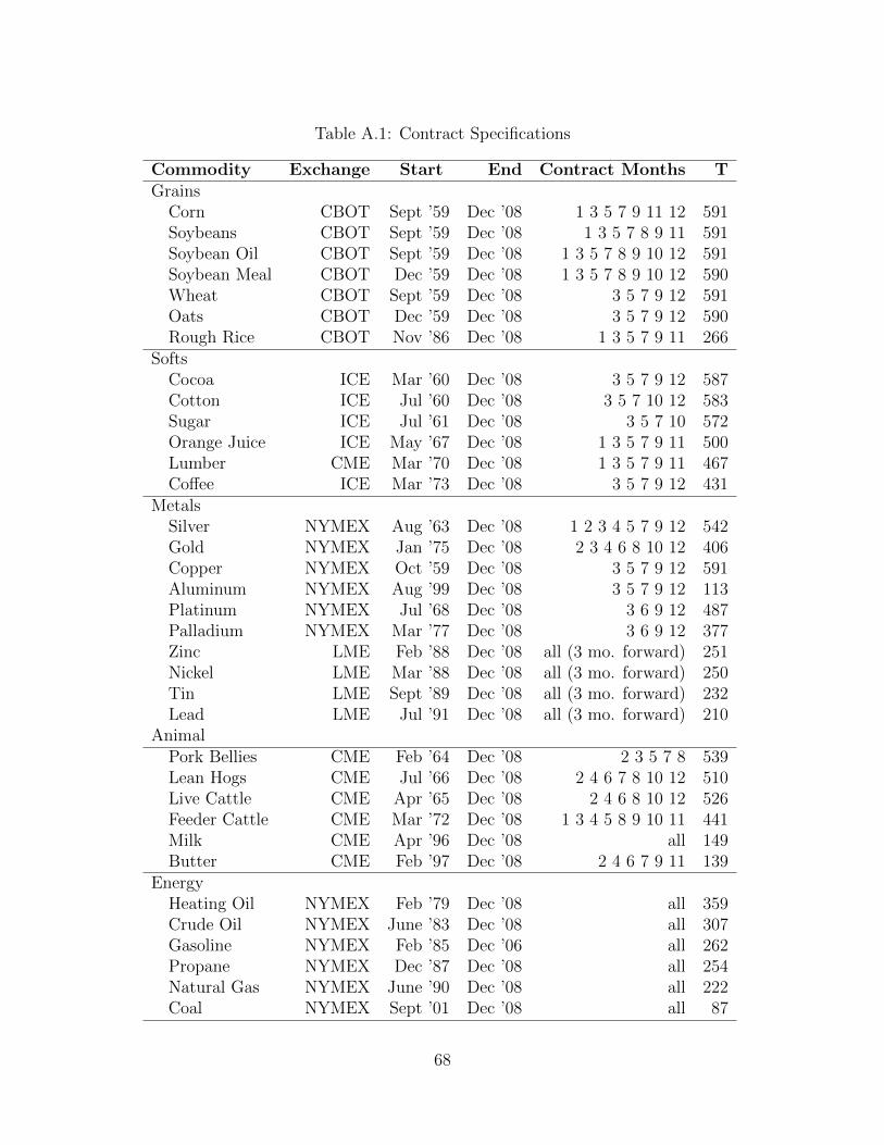
Table A.1: Contract Specifications

Commodity Exchange Start End Contract Months TGrains

Corn CBOT Sept ’59 Dec ’08 1 3 5 7 9 11 12 591Soybeans CBOT Sept ’59 Dec ’08 1 3 5 7 8 9 11 591Soybean Oil CBOT Sept ’59 Dec ’08 1 3 5 7 8 9 10 12 591Soybean Meal CBOT Dec ’59 Dec ’08 1 3 5 7 8 9 10 12 590Wheat CBOT Sept ’59 Dec ’08 3 5 7 9 12 591Oats CBOT Dec ’59 Dec ’08 3 5 7 9 12 590Rough Rice CBOT Nov ’86 Dec ’08 1 3 5 7 9 11 266

SoftsCocoa ICE Mar ’60 Dec ’08 3 5 7 9 12 587Cotton ICE Jul ’60 Dec ’08 3 5 7 10 12 583Sugar ICE Jul ’61 Dec ’08 3 5 7 10 572Orange Juice ICE May ’67 Dec ’08 1 3 5 7 9 11 500Lumber CME Mar ’70 Dec ’08 1 3 5 7 9 11 467Coffee ICE Mar ’73 Dec ’08 3 5 7 9 12 431

MetalsSilver NYMEX Aug ’63 Dec ’08 1 2 3 4 5 7 9 12 542Gold NYMEX Jan ’75 Dec ’08 2 3 4 6 8 10 12 406Copper NYMEX Oct ’59 Dec ’08 3 5 7 9 12 591Aluminum NYMEX Aug ’99 Dec ’08 3 5 7 9 12 113Platinum NYMEX Jul ’68 Dec ’08 3 6 9 12 487Palladium NYMEX Mar ’77 Dec ’08 3 6 9 12 377Zinc LME Feb ’88 Dec ’08 all (3 mo. forward) 251Nickel LME Mar ’88 Dec ’08 all (3 mo. forward) 250Tin LME Sept ’89 Dec ’08 all (3 mo. forward) 232Lead LME Jul ’91 Dec ’08 all (3 mo. forward) 210

AnimalPork Bellies CME Feb ’64 Dec ’08 2 3 5 7 8 539Lean Hogs CME Jul ’66 Dec ’08 2 4 6 7 8 10 12 510Live Cattle CME Apr ’65 Dec ’08 2 4 6 8 10 12 526Feeder Cattle CME Mar ’72 Dec ’08 1 3 4 5 8 9 10 11 441Milk CME Apr ’96 Dec ’08 all 149Butter CME Feb ’97 Dec ’08 2 4 6 7 9 11 139

EnergyHeating Oil NYMEX Feb ’79 Dec ’08 all 359Crude Oil NYMEX June ’83 Dec ’08 all 307Gasoline NYMEX Feb ’85 Dec ’06 all 262Propane NYMEX Dec ’87 Dec ’08 all 254Natural Gas NYMEX June ’90 Dec ’08 all 222Coal NYMEX Sept ’01 Dec ’08 all 87

68

Table A.2: Individual Commodity Summary Statistics

Excess Return Spot Return Basis CorrelationCommodity T Mean Ann. Mean Ann. Mean Ann. All Within

(% p.a.) Vol. (% p.a.) Vol. (% p.a.) Vol. TypeGrains

Corn 591 -2.09 24.33 5.69 25.64 7.87 8.21 0.21 0.57Soybeans 591 5.24 27.85 6.92 28.70 1.64 8.61 0.23 0.57Soybean Oil 591 7.80 32.30 7.19 30.82 0.00 8.91 0.21 0.49Soybean Meal 590 8.68 31.11 8.00 32.05 -0.44 9.73 0.20 0.49Wheat 591 -0.12 25.40 5.56 26.97 5.80 9.49 0.16 0.43Oats 590 -1.22 28.23 6.16 29.61 7.91 11.21 0.14 0.41Rough Rice 266 -0.36 34.60 12.27 39.26 11.88 10.89 0.10 0.23

SoftsCocoa 587 3.91 32.80 7.72 32.29 4.07 8.31 0.11 0.11Cotton 583 1.51 24.64 4.36 26.90 3.00 11.63 0.15 0.05Sugar 572 7.36 48.71 13.80 49.49 7.14 13.94 0.11 0.08Orange Juice 500 4.44 33.07 6.82 33.68 3.08 10.28 0.02 0.00Lumber 467 -1.53 28.37 6.65 30.38 8.68 14.72 0.10 0.04Coffee 431 7.04 41.37 8.73 41.44 2.46 10.81 0.06 0.03

MetalSilver 542 1.70 33.31 9.86 34.14 8.20 4.52 0.21 0.45Gold 406 -0.88 19.93 6.32 20.39 7.27 2.28 0.17 0.37Copper 591 11.52 31.26 7.64 29.81 -3.09 8.49 0.21 0.43Aluminum 487 4.03 28.60 6.70 28.44 3.38 4.09 0.24 0.48Platinum 377 8.33 38.09 11.01 38.23 2.68 3.95 0.20 0.37Palladium 113 2.21 20.06 3.79 20.09 2.27 1.77 0.35 0.58Zinc 251 -2.14 29.70 9.77 36.66 13.17 26.05 0.14 0.38Nickel 250 12.88 45.41 15.11 65.31 -0.41 15.11 0.14 0.32Tin 232 3.00 24.28 4.21 24.02 1.32 3.20 0.22 0.39Lead 210 7.50 31.27 8.80 30.95 1.49 4.89 0.15 0.33

AnimalPork Bellies 539 6.16 32.69 10.70 41.83 7.24 22.20 0.11 0.33Lean Hogs 510 7.08 24.78 6.17 31.10 -0.36 20.60 0.15 0.41Live Cattle 526 6.01 16.94 4.49 18.54 -1.07 9.96 0.15 0.40Feeder Cattle 441 3.72 16.36 4.20 17.66 0.60 6.57 0.12 0.35Milk 149 10.17 32.19 6.58 37.27 -1.93 22.11 0.09 0.22Butter 139 9.66 34.36 11.96 35.60 4.36 12.83 -0.03 0.14

EnergyHeating Oil 359 13.56 35.72 10.32 37.26 -1.94 14.38 0.16 0.72Crude Oil 307 14.12 35.19 8.81 36.38 -5.07 8.32 0.18 0.69Gasoline 262 20.50 35.71 10.40 38.19 -9.35 16.33 0.10 0.63Propane 254 22.94 49.09 16.85 52.47 -6.97 14.36 0.14 0.63Natural Gas 222 8.09 48.95 22.38 56.83 15.07 31.20 0.12 0.46Coal 87 5.61 35.57 15.90 37.14 9.07 9.78 0.30 0.48

Notes: ∗p < 0.10, ∗∗p < 0.05, and ∗∗∗p < 0.01. Excess returns are calculated as(St − Ft−3,t)/Ft−3,t. Volatilities, standard errors, and p-values are calculated using Newey-West standard errors with 4 lags. Reported multiple betas are estimated using a separate timeseries regression for each portfolio: Reit = βi0 + βic∆ct + βid∆dt + βiwrWt + εit.

69

Tab

leA

.3:

Typ

eP

ortf

olio

Sum

mar

ySta

tist

ics

Mea

nP

ortf

olio

Cor

rela

tion

Avg.

Cor

r.A

uto

corr

elat

ion

Por

tfol

io(%

p.a

.)G

rain

sSof

tsM

etal

Anim

alE

ner

gy(w

ithin

typ

e)1

mon

th3

mon

thT

Gra

ins

2.93

..

..

.0.

450.

670.

0559

1Sof

ts3.

500.

35.

..

.0.

050.

690.

1058

3M

etal

6.27

*0.

220.

34.

..

0.41

0.70

0.13

542

Anim

al6.

16**

0.26

0.04

0.14

..

0.31

0.67

-0.0

252

6E

ner

gy14

.32*

*0.

020.

090.

230.

08.

0.60

0.65

0.00

307

All

Com

modit

ies

5.69

***

0.72

0.63

0.65

0.45

0.58

0.15

0.70

0.10

591

Not

es:

∗ p<

0.1

0,∗∗p<

0.05

,an

d∗∗

∗ p<

0.01.

Sta

nd

ard

erro

rsare

calc

ula

ted

usi

ng

New

ey-W

est

stan

dard

erro

rsw

ith

4la

gs.

Ave

rage

corr

elat

ion

wit

hin

typ

em

easu

res

the

aver

age

pair

wis

eco

rrel

ati

on

am

on

gall

pair

sof

com

mod

itie

sw

ith

ina

giv

enty

pe.

Tab

leA

.4:

Fac

tor

Sum

mar

ySta

tist

ics

Mea

nA

nn.

Shar

pe

Auto

corr

elat

ion

Fac

tor

Cor

rela

tion

(%p.a

.)V

ol.

Rat

io1

mon

th3

mon

th(rWt)

(∆c t

)(∆dt)

Mar

ket

Ret

urn

s(rWt)

4.94

**15

.88

0.31

0.70

0.05

..

.N

ondura

ble

Con

sum

pti

on(∆c t

)2.

08**

*1.

061.

960.

610.

170.

18.

.D

ura

ble

Con

sum

pti

on(∆dt)

3.94

***

1.14

3.45

0.98

0.91

0.03

0.28

.A

llC

omm

odit

ies

5.69

***

13.5

80.

420.

700.

100.

070.

000.

22

Not

es:

∗ p<

0.10

,∗∗p<

0.0

5,an

d∗∗

∗ p<

0.01.

Sta

nd

ard

erro

rsan

dvola

tili

ties

are

calc

ula

ted

usi

ng

New

ey-W

est

stan

dard

erro

rsw

ith

4la

gs.

70

Table A.5: Portfolio Characteristics Over Time

T Excess Return Risk AmountMean Ann. Sharpe Multiple Betas(% p.a.) Volatility Ratio p-value βw βc βd

Panel A1: Full Sample (Oct ’59-Dec ’08)Grains 591 2.93 21.75 0.14 0.31 -0.07 -1.07 2.39Softs 583 3.50 17.89 0.20 0.15 0.10 -0.55 2.09**Metal 542 6.27* 24.19 0.26 0.07 0.30*** -0.79 4.80***Animal 526 6.16** 18.91 0.33 0.02 0.06 0.14 3.09**Energy 307 14.32** 33.20 0.43 0.02 -0.12 -5.86* 4.18All Commodities 591 5.69*** 13.58 0.42 0.00 0.07 -1.11 2.96***Panel A2: Early Sample (Oct ’59-Dec ’83)Grains 291 6.63 23.72 0.28 0.14 -0.18 -2.95* 4.92**Softs 283 8.22* 21.06 0.39 0.05 0.15 -2.69* 4.95***Metal 242 9.78 30.42 0.32 0.13 0.40** -2.68 7.02***Animal 226 9.16** 22.33 0.41 0.05 -0.02 1.17 4.96**Energy 7 – – – – – – –All Commodities 291 7.87*** 15.34 0.51 0.01 0.06 -2.11* 4.61***Panel A3: Late Sample (Jan ’84 - Dec ’08)Grains 300 -0.66 19.52 -0.03 0.86 0.06 1.15 -0.09Softs 300 -0.95 13.96 -0.07 0.70 0.08 1.51 -0.19Metal 300 3.44 17.57 0.20 0.32 0.25* 0.42 3.65**Animal 300 3.90 15.80 0.25 0.18 0.14** -2.28** 2.33Energy 300 14.64** 33.52 0.44 0.02 -0.13 -6.32* 4.57All Commodities 300 3.58 11.57 0.31 0.12 0.09 -0.59 2.00

Notes: ∗p < 0.10, ∗∗p < 0.05, and ∗∗∗p < 0.01. Standard errors are calculated using Newey-Weststandard errors with 4 lags. Reported multiple betas are estimated using a separate time seriesregression for each commodity: Reit = βi0 + βic∆ct + βid∆dt + βiwrWt + εit.

71

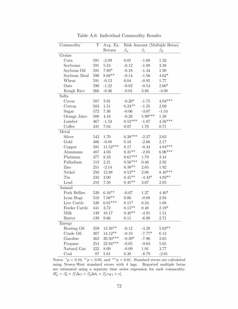
Table A.6: Individual Commodity Results

Commodity T Avg. Ex. Risk Amount (Multiple Betas)Return βw βc βd

GrainsCorn 591 -2.09 0.01 -1.60 1.33Soybeans 591 5.24 -0.12 -1.08 3.38Soybean Oil 591 7.80* -0.18 -1.34 1.90Soybean Meal 590 8.68** -0.14 -1.56 4.62*Wheat 591 -0.12 0.04 -0.95 1.77Oats 590 -1.22 -0.02 -0.54 2.60*Rough Rice 266 -0.36 -0.01 3.86 -3.08

SoftsCocoa 587 3.91 -0.20* -1.75 4.94***Cotton 583 1.51 0.24** -1.35 2.09Sugar 572 7.36 -0.06 -3.07 -1.54Orange Juice 500 4.44 -0.20 5.99*** 1.38Lumber 467 -1.53 0.52*** -1.07 4.56***Coffee 431 7.04 0.07 1.78 0.71

MetalSilver 542 1.70 0.38*** -2.27 2.63Gold 406 -0.88 0.10 -2.66 2.17Copper 591 11.52*** 0.17 -0.44 4.84***Aluminum 487 4.03 0.31** -2.05 6.96***Platinum 377 8.33 0.61*** 1.79 3.44Palladium 113 2.21 0.56*** 0.46 2.92Zinc 251 -2.14 0.38** 2.65 1.92Nickel 250 12.88 0.53** 2.08 8.40***Tin 232 3.00 0.45** -4.43* 4.93**Lead 210 7.50 0.45** 3.67 2.85

AnimalPork Bellies 539 6.16** -0.07 1.27 4.40*Lean Hogs 510 7.08** 0.06 -0.88 2.94Live Cattle 526 6.01*** 0.11* 0.24 1.68Feeder Cattle 441 3.72 0.15** 0.48 2.19*Milk 149 10.17 0.40** -4.91 1.51Butter 139 9.66 0.11 -6.90 2.71

EnergyHeating Oil 359 13.56** -0.12 -4.28 5.03**Crude Oil 307 14.12** -0.10 -7.77* 6.13Gasoline 262 20.50*** -0.39* -7.96 2.65Propane 254 22.94*** -0.05 -9.63 5.65Natural Gas 222 8.09 -0.09 1.91 3.77Coal 87 5.61 0.38 -8.79 -2.01

Notes: ∗p < 0.10, ∗∗p < 0.05, and ∗∗∗p < 0.01. Standard errors are calculatedusing Newey-West standard errors with 4 lags. Reported multiple betasare estimated using a separate time series regression for each commodity:Reit = βi0 + βic∆ct + βid∆dt + βiwrWt + εit.

72

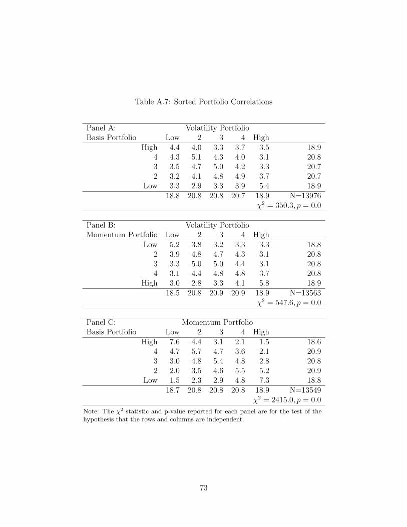
Table A.7: Sorted Portfolio Correlations

Panel A: Volatility PortfolioBasis Portfolio Low 2 3 4 High

High 4.4 4.0 3.3 3.7 3.5 18.94 4.3 5.1 4.3 4.0 3.1 20.83 3.5 4.7 5.0 4.2 3.3 20.72 3.2 4.1 4.8 4.9 3.7 20.7

Low 3.3 2.9 3.3 3.9 5.4 18.918.8 20.8 20.8 20.7 18.9 N=13976

χ2 = 350.3, p = 0.0

Panel B: Volatility PortfolioMomentum Portfolio Low 2 3 4 High

Low 5.2 3.8 3.2 3.3 3.3 18.82 3.9 4.8 4.7 4.3 3.1 20.83 3.3 5.0 5.0 4.4 3.1 20.84 3.1 4.4 4.8 4.8 3.7 20.8

High 3.0 2.8 3.3 4.1 5.8 18.918.5 20.8 20.9 20.9 18.9 N=13563

χ2 = 547.6, p = 0.0

Panel C: Momentum PortfolioBasis Portfolio Low 2 3 4 High

High 7.6 4.4 3.1 2.1 1.5 18.64 4.7 5.7 4.7 3.6 2.1 20.93 3.0 4.8 5.4 4.8 2.8 20.82 2.0 3.5 4.6 5.5 5.2 20.9

Low 1.5 2.3 2.9 4.8 7.3 18.818.7 20.8 20.8 20.8 18.9 N=13549

χ2 = 2415.0, p = 0.0

Note: The χ2 statistic and p-value reported for each panel are for the test of thehypothesis that the rows and columns are independent.

73

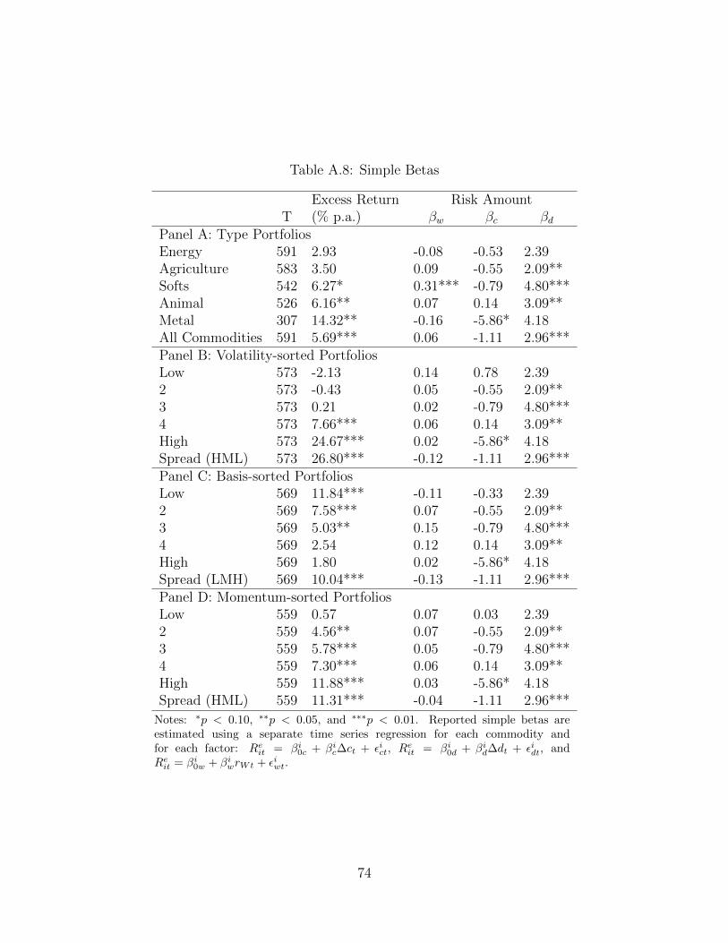
Table A.8: Simple Betas

Excess Return Risk AmountT (% p.a.) βw βc βd

Panel A: Type PortfoliosEnergy 591 2.93 -0.08 -0.53 2.39Agriculture 583 3.50 0.09 -0.55 2.09**Softs 542 6.27* 0.31*** -0.79 4.80***Animal 526 6.16** 0.07 0.14 3.09**Metal 307 14.32** -0.16 -5.86* 4.18All Commodities 591 5.69*** 0.06 -1.11 2.96***Panel B: Volatility-sorted PortfoliosLow 573 -2.13 0.14 0.78 2.392 573 -0.43 0.05 -0.55 2.09**3 573 0.21 0.02 -0.79 4.80***4 573 7.66*** 0.06 0.14 3.09**High 573 24.67*** 0.02 -5.86* 4.18Spread (HML) 573 26.80*** -0.12 -1.11 2.96***Panel C: Basis-sorted PortfoliosLow 569 11.84*** -0.11 -0.33 2.392 569 7.58*** 0.07 -0.55 2.09**3 569 5.03** 0.15 -0.79 4.80***4 569 2.54 0.12 0.14 3.09**High 569 1.80 0.02 -5.86* 4.18Spread (LMH) 569 10.04*** -0.13 -1.11 2.96***Panel D: Momentum-sorted PortfoliosLow 559 0.57 0.07 0.03 2.392 559 4.56** 0.07 -0.55 2.09**3 559 5.78*** 0.05 -0.79 4.80***4 559 7.30*** 0.06 0.14 3.09**High 559 11.88*** 0.03 -5.86* 4.18Spread (HML) 559 11.31*** -0.04 -1.11 2.96***

Notes: ∗p < 0.10, ∗∗p < 0.05, and ∗∗∗p < 0.01. Reported simple betas areestimated using a separate time series regression for each commodity andfor each factor: Reit = βi0c + βic∆ct + εict, Reit = βi0d + βid∆dt + εidt, andReit = βi0w + βiwrWt + εiwt.

74

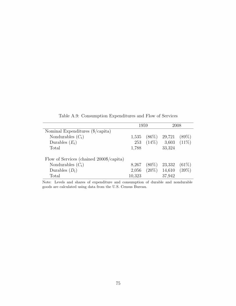
Table A.9: Consumption Expenditures and Flow of Services

1959 2008Nominal Expenditures ($/capita)

Nondurables (Ct) 1,535 (86%) 29,721 (89%)Durables (Et) 253 (14%) 3,603 (11%)Total 1,788 33,324

Flow of Services (chained 2000$/capita)Nondurables (Ct) 8,267 (80%) 23,332 (61%)Durables (Dt) 2,056 (20%) 14,610 (39%)Total 10,323 37,942

Note: Levels and shares of expenditure and consumption of durable and nondurablegoods are calculated using data from the U.S. Census Bureau.

75