Consumption-Based Asset Pricing: Durable Goods, Adjustment Costs, and

Aggregation

Abstract

In this paper, we investigate the implications of non-separable preferences over durable and nondurable consumption for asset pricing tests when adjusting durable consumption is costly. In an economy without adjustment costs, in which a frictionless rental market exists for the durable good, the standard Euler equation with respect to nondurable consumption will hold for each individual agent as well as for aggregate data. If the adjustment of the durable good is costly, however, aggregation generally fails. We use aggregate data to find substantial deviations from the frictionless model, consistent with the presence of non-convex adjustment costs for the durable good. We also show how empirical asset pricing tests that use aggregate data can be affected by these deviations. We then propose and implement asset pricing tests that are robust to the presence of adjustment costs by relying on microeconomic data. Using household-level observations of nondurable food and durable housing consumption, our estimation results suggest that preferences are indeed non-separable in the two consumption goods and that reasonable structural parameters characterize agents' intertemporal utility optimizations.

1 Introduction

Consumption-based asset pricing models, despite their many empirical failures, have been

at the heart of asset pricing research for over two decades. Naturally, the starting point

of these models is a particular assumption on what consumption is and here researchers

have, for the most part, restricted themselves to measuring consumption as consumption

of nondurable goods and services. Recently though, there has been renewed interest in

an old topic, namely the role of durable consumption in asset pricing tests.1 Introducing

durable consumption into the agent’s utility function brings new modelling issues to the

asset pricing literature. One such issue is whether changing durable consumption is subject

to adjustment costs and how these adjustment costs potentially affect asset prices. This

question is particularly important if one uses aggregate data to test asset pricing implications.

On the one hand, standard aggregation arguments will generally not hold if individual agents

are subject to adjustment costs. Asset pricing tests using aggregate data therefore risk being

misspecified if they do not account for consumption heterogeneity across individual agents.

On the other hand, however, aggregation introduces smoothness that could make infrequent

adjustments at the micro level irrelevant for understanding aggregate phenomena. In other

words, macroeconomic data might behave as if generated by a representative agent in a

frictionless economy. In this paper we therefore investigate whether asset pricing tests that

use aggregate data can safely ignore adjustment costs, either because they are irrelevant at

the individual level or, more likely, because frictions at the micro level do not affect the

relationship between aggregate data and asset returns.

Our tests rely on the fact that in a frictionless economy with a rental market for the

durable good, the ratio of marginal utilities with respect to the two consumption goods

equals the relative user cost at any point in time. By analyzing the implied cointegration

relationship between durable and nondurable consumption and the relative user cost for ag-

gregate data, we are able to determine whether the data are consistent with the assumption

1See Dunn and Singleton (1986) and Eichenbaum and Hansen (1990) for early work on this topic. See

Piazessi, Schneider, and Tuzel (2006), Pakos (2003), Yogo (2006) and Lustig and Van Nieuwerburgh (2005)

for recent work.

1

of a representative agent that can adjust his durable consumption costlessly. Our empirical

results suggest that this is not the case. Moreover, we find that deviations from the coin-

tegration relationship contain information about asset returns, indicating that the standard

Euler equation with respect to nondurable consumption does not hold in aggregate data. At

the same time, though, the Euler equation still has to hold at the individual level, even if

non-convex adjustment costs with respect to the durable good are present. In the second

part of the paper, we therefore use micro-level data to evaluate a model with non-separable

preferences and adjustment costs. Unlike models estimated from aggregate data, we obtain

reasonable structural estimates. The variability of the implied pricing kernel in our model

is, however, still too low to to be reconciled with the observed US equity premium.

Early empirical work on aggregate data by Dunn and Singleton (1986) and Eichenbaum

and Hansen (1990) finds that non-separable preferences over durable and nondurable con-

sumption do not significantly improve asset pricing models based on nondurable consumption

only. Piazessi, Schneider, and Tuzel (2006), however, show that a representative agent with

CES preferences over nondurable and housing service consumption implies an Euler equation

that after linearization is consistent with observed equity returns. Focusing on services from

durable goods such as vehicles and furniture, Yogo (2006) finds that such a model is able

to price the cross-section of equity excess returns. Finally, Lustig and Van Nieuwerburgh

(2005) study a model with bankruptcy similar to the one in Piazzesi et. al. (2006), where

the housing good serves as collateral. They find that the aggregate housing stock to income

ratio helps to explain time series as well as cross-sectional variation of equity returns. All

these papers assume that there are no frictions with respect to the durable good and that

standard first order conditions can be tested on aggregate data.

There is substantial empirical evidence in the economics literature, however, that durable

goods are subject to non-convex adjustment costs. Eberly (1994) finds that expenditures

on private vehicles are consistent with models of non-convex adjustments costs. Similarly,

Caballero (1993), Carroll and Dunn (1997), and Attanasio (2000) provide evidence that

the time series dynamics of aggregate durable purchases can better be explained by models

in which individuals face non-convex adjustment costs than by frictionless models. Kull-

2

mann and Siegel (2005) study homeowners’ portfolio choices and find them to be consistent

with state-dependent risk aversion, as implied by a model with non-convex adjustment costs

with respect to residential housing. Grossman and Laroque (1990), Beaulieu (1992), and

Damgaard, Fuglsbjerg, and Munk (2000) study partial equilibrium models in which an indi-

vidual consumer faces non-convex costs for adjusting the size of the durable good. Continuous

adjustment of the durable good is infinitely expensive, resulting in infrequent adjustments

of the durable good stock. In this case, the ratio of marginal utilities of the two goods is no

longer equated to the relative user cost at every moment. This deviation from the frictionless

model provides the motivation for the empirical tests in the first part of this paper.

Marshall and Parekh (1999) explore the consequences of adjustment costs for asset prices

when preferences are separable across different consumption goods. They find that ad-

justment costs with respect to nondurable consumption can partially reconcile nondurable

consumption data with the observed equity premium. However, several empirical papers

suggest that the separability between durable and nondurable consumption is difficult to

maintain. Eichenbaum and Hansen’s (1990) analysis with macroeconomic data supports the

assumption that preferences over nondurable and durable good consumption are not sep-

arable. Using household-level data to explicitly account for non-convex adjustment costs,

Martin (2001) also finds support for non-separability. If preferences are non-separable, ad-

justment costs for the durable good have a direct impact on the marginal utility with respect

to both durable and nondurable consumption. When different agents adjust their durable

stock at different points in time, we can no longer aggregate across individuals to use a

representative agent framework. That is, even though the Euler equation with respect to

nondurable consumption will continue to hold for every individual agent, it will generally not

hold for aggregate consumption data. This motivates the use of micro-level data to perform

asset pricing tests in the second part of the paper.

Household-level data have been used in recent studies to explore market incompleteness

and idiosyncratic risks when preferences are separable in the two consumption goods. Among

those, Jacobs (1999) is most related to our estimation approach. In the permanent income

hypothesis literature, a few panel data studies have included durable goods in their tests.

3

Hayashi (1985) and Padula (1999) find that the inclusion of durable goods improves the

performance of their models. Following the tradition of the saving-consumption literature,

however, they focus exclusively on the Euler equation with respect to the risk-free asset.

Since they do not assume a specific form for their utility function, they furthermore do not

provide estimates of structural preference parameters. In a current research paper, Flavin

and Nakagawa (2004) use a micro-level data set similar to ours to study non-separable

preferences in a somewhat different setting. We discuss their findings together with our own

results at the end of the second part of the paper.

The remainder of this paper is organized as follows. The next section presents the

underlying model for an economy with and without adjustment costs and discusses the

consequences for aggregation and empirical asset pricing tests. In Section 3, we test for the

presence of adjustment costs using macroeconomic data. To account for the existence of

adjustment costs, Section 4 presents asset pricing tests performed on household level data.

Section 5 concludes.

2 Model

We first describe a simple frictionless economy with many agents that differ only in their

relative endowments of the durable good. We show that if the durable good can be adjusted

costlessly, this initial heterogeneity is without consequence: Aggregation across agents is

straightforward and empirical asset pricing tests can be carried out on macroeconomic con-

sumption data. We then introduce non-convex adjustment costs with respect to the durable

good to show that aggregation across agents is no longer trivial.

2.1 The frictionless economy

To be specific, suppose N agents, subscripted i = 1, ..., N , have identical preferences that

are non-separable in a nondurable consumption good Ci,t and the service flow Si,t from a

durable good Di,t. For simplicity, we assume the service flow to be proportional to the size

4

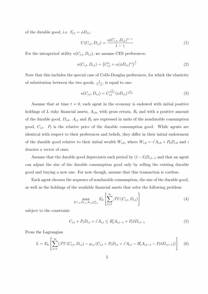
of the durable good, i.e. Si,t = φDi,t:

U(Ci,t, Di,t) =u(Ci,t, Di,t)

1−γ

1− γ(1)

For the intraperiod utility u(Ci,t, Di,t), we assume CES preferences:

u(Ci,t, Di,t) =(Cω

i,t + α(φDi,t)ω) 1

ω (2)

Note that this includes the special case of Cobb-Douglas preferences, for which the elasticity

of substitution between the two goods, 11−ω

, is equal to one:

u(Ci,t, Di,t) = C1

1+α

i,t (φDi,t)α

1+α (3)

Assume that at time t = 0, each agent in the economy is endowed with initial positive

holdings of L risky financial assets, Ai,0, with gross return, Rt and with a positive amount

of the durable good, Di,0. Ai,t and Rt are expressed in units of the nondurable consumption

good, Ci,t. Pt is the relative price of the durable consumption good. While agents are

identical with respect to their preferences and beliefs, they differ in their initial endowment

of the durable good relative to their initial wealth Wi,0, where Wi,0 = ı′Ai,0 + P0Di,0 and ı

denotes a vector of ones.

Assume that the durable good depreciates each period by (1−δ)Di,t−1 and that an agent

can adjust the size of the durable consumption good only by selling the existing durable

good and buying a new one. For now though, assume that this transaction is costless.

Each agent chooses the sequence of nondurable consumption, the size of the durable good,

as well as the holdings of the available financial assets that solve the following problem:

max{Ci,t,Di,t,Ai,t}∞t=1

E0

[ ∞∑t=1

βtU(Ci,t, Di,t)

](4)

subject to the constraint:

Ci,t + PtDi,t + ı′Ai,t ≤ R′tAi,t−1 + PtδDi,t−1 (5)

From the Lagrangian

L = E0

[ ∞∑t=1

(βtU(Ci,t, Di,t)− µi,t (Ci,t + PtDi,t + ı′Ai,t −R′tAi,t−1 − PtδDi,t−1))

](6)

5

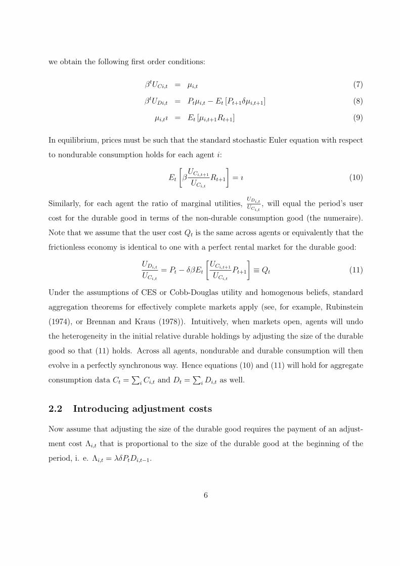
we obtain the following first order conditions:

βtUCi,t = µi,t (7)

βtUDi,t = Ptµi,t − Et [Pt+1δµi,t+1] (8)

µi,tı = Et [µi,t+1Rt+1] (9)

In equilibrium, prices must be such that the standard stochastic Euler equation with respect

to nondurable consumption holds for each agent i:

Et

[β

UCi,t+1

UCi,t

Rt+1

]= ı (10)

Similarly, for each agent the ratio of marginal utilities,UDi,t

UCi,t, will equal the period’s user

cost for the durable good in terms of the non-durable consumption good (the numeraire).

Note that we assume that the user cost Qt is the same across agents or equivalently that the

frictionless economy is identical to one with a perfect rental market for the durable good:

UDi,t

UCi,t

= Pt − δβEt

[UCi,t+1

UCi,t

Pt+1

]≡ Qt (11)

Under the assumptions of CES or Cobb-Douglas utility and homogenous beliefs, standard

aggregation theorems for effectively complete markets apply (see, for example, Rubinstein

(1974), or Brennan and Kraus (1978)). Intuitively, when markets open, agents will undo

the heterogeneity in the initial relative durable holdings by adjusting the size of the durable

good so that (11) holds. Across all agents, nondurable and durable consumption will then

evolve in a perfectly synchronous way. Hence equations (10) and (11) will hold for aggregate

consumption data Ct =∑

i Ci,t and Dt =∑

i Di,t as well.

2.2 Introducing adjustment costs

Now assume that adjusting the size of the durable good requires the payment of an adjust-

ment cost Λi,t that is proportional to the size of the durable good at the beginning of the

period, i. e. Λi,t = λδPtDi,t−1.

6

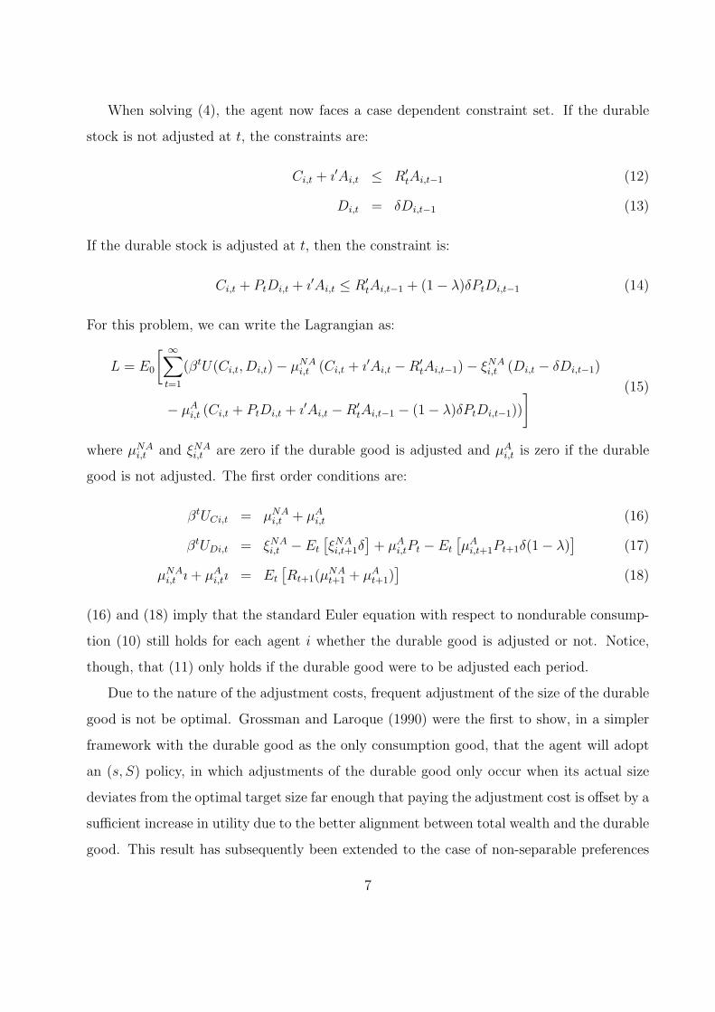
When solving (4), the agent now faces a case dependent constraint set. If the durable

stock is not adjusted at t, the constraints are:

Ci,t + ı′Ai,t ≤ R′tAi,t−1 (12)

Di,t = δDi,t−1 (13)

If the durable stock is adjusted at t, then the constraint is:

Ci,t + PtDi,t + ı′Ai,t ≤ R′tAi,t−1 + (1− λ)δPtDi,t−1 (14)

For this problem, we can write the Lagrangian as:

L = E0

[ ∞∑t=1

(βtU(Ci,t, Di,t)− µNAi,t (Ci,t + ı′Ai,t −R′

tAi,t−1)− ξNAi,t (Di,t − δDi,t−1)

− µAi,t (Ci,t + PtDi,t + ı′Ai,t −R′

tAi,t−1 − (1− λ)δPtDi,t−1))

] (15)

where µNAi,t and ξNA

i,t are zero if the durable good is adjusted and µAi,t is zero if the durable

good is not adjusted. The first order conditions are:

βtUCi,t = µNAi,t + µA

i,t (16)

βtUDi,t = ξNAi,t − Et

[ξNAi,t+1δ

]+ µA

i,tPt − Et

[µA

i,t+1Pt+1δ(1− λ)]

(17)

µNAi,t ı + µA

i,tı = Et

[Rt+1(µ

NAt+1 + µA

t+1)]

(18)

(16) and (18) imply that the standard Euler equation with respect to nondurable consump-

tion (10) still holds for each agent i whether the durable good is adjusted or not. Notice,

though, that (11) only holds if the durable good were to be adjusted each period.

Due to the nature of the adjustment costs, frequent adjustment of the size of the durable

good is not be optimal. Grossman and Laroque (1990) were the first to show, in a simpler

framework with the durable good as the only consumption good, that the agent will adopt

an (s, S) policy, in which adjustments of the durable good only occur when its actual size

deviates from the optimal target size far enough that paying the adjustment cost is offset by a

sufficient increase in utility due to the better alignment between total wealth and the durable

good. This result has subsequently been extended to the case of non-separable preferences

7

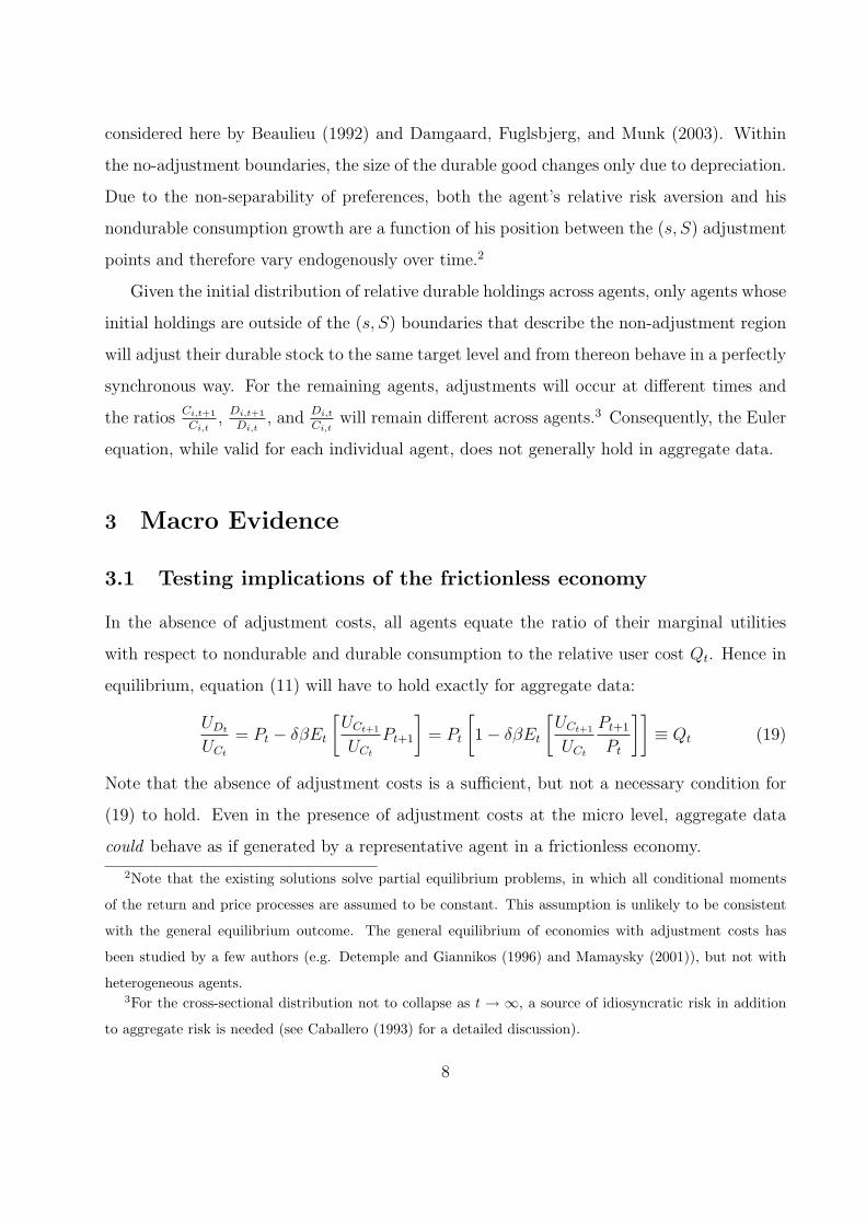
considered here by Beaulieu (1992) and Damgaard, Fuglsbjerg, and Munk (2003). Within

the no-adjustment boundaries, the size of the durable good changes only due to depreciation.

Due to the non-separability of preferences, both the agent’s relative risk aversion and his

nondurable consumption growth are a function of his position between the (s, S) adjustment

points and therefore vary endogenously over time.2

Given the initial distribution of relative durable holdings across agents, only agents whose

initial holdings are outside of the (s, S) boundaries that describe the non-adjustment region

will adjust their durable stock to the same target level and from thereon behave in a perfectly

synchronous way. For the remaining agents, adjustments will occur at different times and

the ratiosCi,t+1

Ci,t,

Di,t+1

Di,t, and

Di,t

Ci,twill remain different across agents.3 Consequently, the Euler

equation, while valid for each individual agent, does not generally hold in aggregate data.

3 Macro Evidence

3.1 Testing implications of the frictionless economy

In the absence of adjustment costs, all agents equate the ratio of their marginal utilities

with respect to nondurable and durable consumption to the relative user cost Qt. Hence in

equilibrium, equation (11) will have to hold exactly for aggregate data:

UDt

UCt

= Pt − δβEt

[UCt+1

UCt

Pt+1

]= Pt

[1− δβEt

[UCt+1

UCt

Pt+1

Pt

]]≡ Qt (19)

Note that the absence of adjustment costs is a sufficient, but not a necessary condition for

(19) to hold. Even in the presence of adjustment costs at the micro level, aggregate data

could behave as if generated by a representative agent in a frictionless economy.

2Note that the existing solutions solve partial equilibrium problems, in which all conditional moments

of the return and price processes are assumed to be constant. This assumption is unlikely to be consistent

with the general equilibrium outcome. The general equilibrium of economies with adjustment costs has

been studied by a few authors (e.g. Detemple and Giannikos (1996) and Mamaysky (2001)), but not with

heterogeneous agents.3For the cross-sectional distribution not to collapse as t → ∞, a source of idiosyncratic risk in addition

to aggregate risk is needed (see Caballero (1993) for a detailed discussion).

8

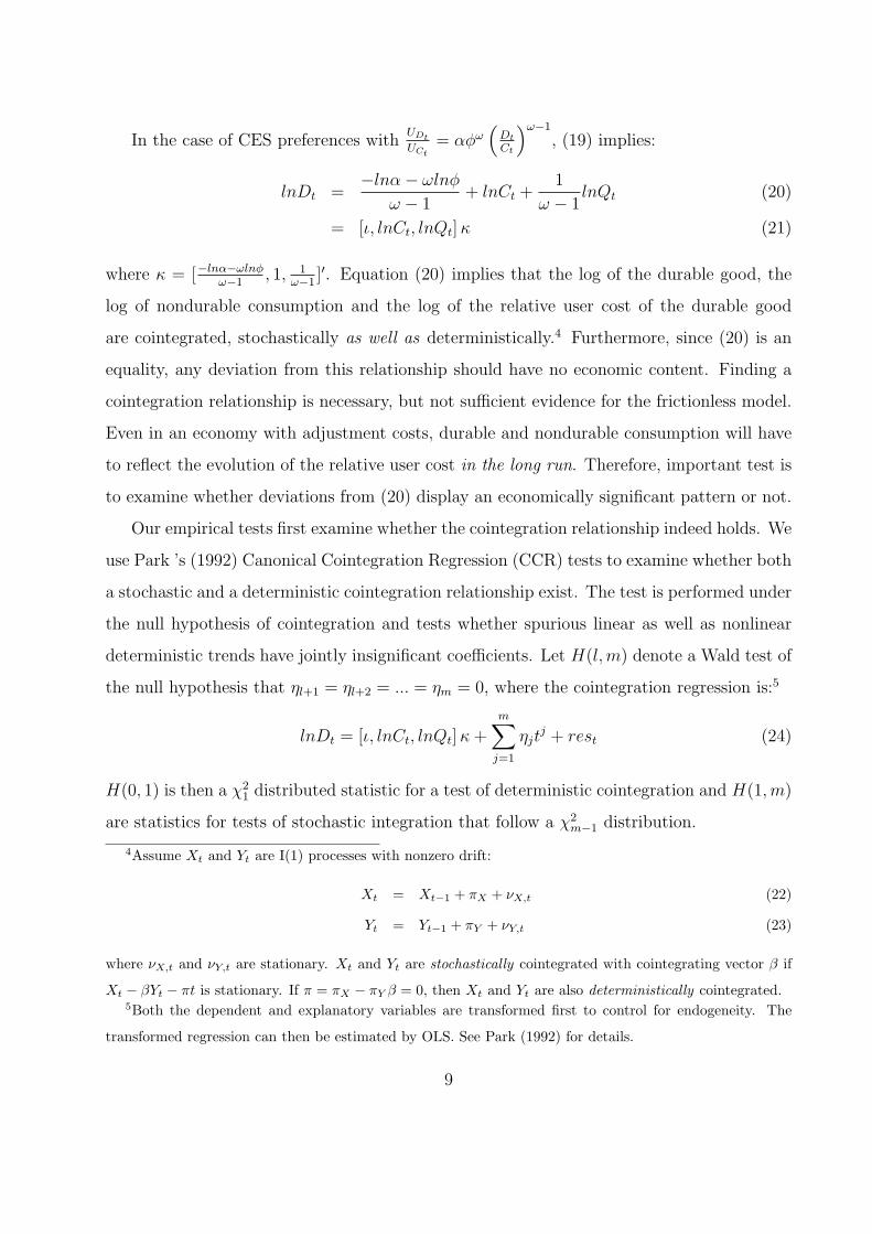
In the case of CES preferences withUDt

UCt= αφω

(Dt

Ct

)ω−1

, (19) implies:

lnDt =−lnα− ωlnφ

ω − 1+ lnCt +

1

ω − 1lnQt (20)

= [ι, lnCt, lnQt] κ (21)

where κ = [−lnα−ωlnφω−1

, 1, 1ω−1

]′. Equation (20) implies that the log of the durable good, the

log of nondurable consumption and the log of the relative user cost of the durable good

are cointegrated, stochastically as well as deterministically.4 Furthermore, since (20) is an

equality, any deviation from this relationship should have no economic content. Finding a

cointegration relationship is necessary, but not sufficient evidence for the frictionless model.

Even in an economy with adjustment costs, durable and nondurable consumption will have

to reflect the evolution of the relative user cost in the long run. Therefore, important test is

to examine whether deviations from (20) display an economically significant pattern or not.

Our empirical tests first examine whether the cointegration relationship indeed holds. We

use Park ’s (1992) Canonical Cointegration Regression (CCR) tests to examine whether both

a stochastic and a deterministic cointegration relationship exist. The test is performed under

the null hypothesis of cointegration and tests whether spurious linear as well as nonlinear

deterministic trends have jointly insignificant coefficients. Let H(l, m) denote a Wald test of

the null hypothesis that ηl+1 = ηl+2 = ... = ηm = 0, where the cointegration regression is:5

lnDt = [ι, lnCt, lnQt] κ +m∑

j=1

ηjtj + rest (24)

H(0, 1) is then a χ21 distributed statistic for a test of deterministic cointegration and H(1,m)

are statistics for tests of stochastic integration that follow a χ2m−1 distribution.

4Assume Xt and Yt are I(1) processes with nonzero drift:

Xt = Xt−1 + πX + νX,t (22)

Yt = Yt−1 + πY + νY,t (23)

where νX,t and νY,t are stationary. Xt and Yt are stochastically cointegrated with cointegrating vector β if

Xt − βYt − πt is stationary. If π = πX − πY β = 0, then Xt and Yt are also deterministically cointegrated.5Both the dependent and explanatory variables are transformed first to control for endogeneity. The

transformed regression can then be estimated by OLS. See Park (1992) for details.

9

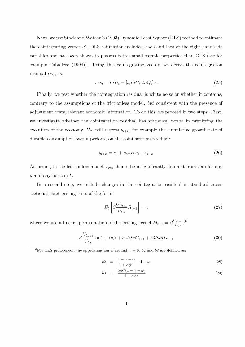
Next, we use Stock and Watson’s (1993) Dynamic Least Square (DLS) method to estimate

the cointegrating vector κ′. DLS estimation includes leads and lags of the right hand side

variables and has been shown to possess better small sample properties than OLS (see for

example Caballero (1994)). Using this cointegrating vector, we derive the cointegration

residual rest as:

rest = lnDt − [ι, lnCt, lnQt] κ (25)

Finally, we test whether the cointegration residual is white noise or whether it contains,

contrary to the assumptions of the frictionless model, but consistent with the presence of

adjustment costs, relevant economic information. To do this, we proceed in two steps. First,

we investigate whether the cointegration residual has statistical power in predicting the

evolution of the economy. We will regress yt+k, for example the cumulative growth rate of

durable consumption over k periods, on the cointegration residual:

yt+k = c0 + cresrest + εt+k (26)

According to the frictionless model, cres should be insignificantly different from zero for any

y and any horizon k.

In a second step, we include changes in the cointegration residual in standard cross-

sectional asset pricing tests of the form:

Et

[β

UCt+1

UCt

Rt+1

]= ı (27)

where we use a linear approximation of the pricing kernel Mt+1 = βUCt+1

UCt:6

βUCt+1

UCt

≈ 1 + lnβ + b2∆lnCt+1 + b3∆lnDt+1 (30)

6For CES preferences, the approximation is around ω = 0. b2 and b3 are defined as:

b2 =1− γ − ω

1 + αφω− 1 + ω (28)

b3 =αφω(1− γ − ω)

1 + αφω(29)

10

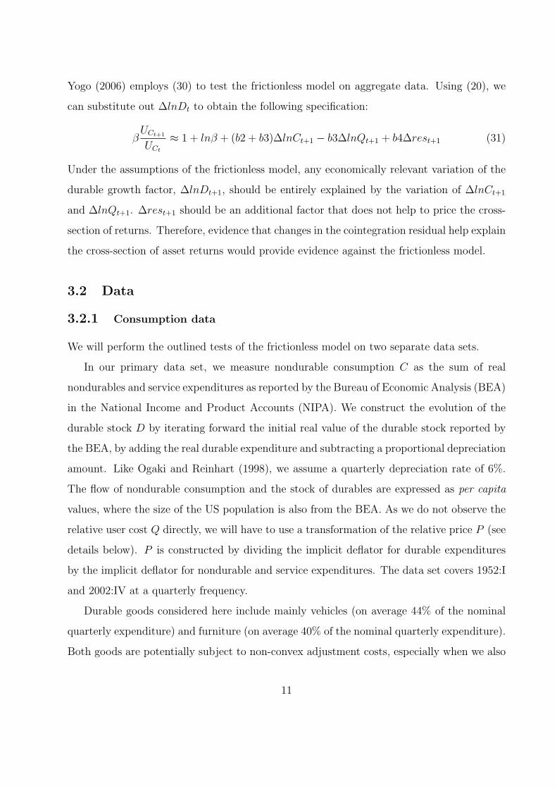
Yogo (2006) employs (30) to test the frictionless model on aggregate data. Using (20), we

can substitute out ∆lnDt to obtain the following specification:

βUCt+1

UCt

≈ 1 + lnβ + (b2 + b3)∆lnCt+1 − b3∆lnQt+1 + b4∆rest+1 (31)

Under the assumptions of the frictionless model, any economically relevant variation of the

durable growth factor, ∆lnDt+1, should be entirely explained by the variation of ∆lnCt+1

and ∆lnQt+1. ∆rest+1 should be an additional factor that does not help to price the cross-

section of returns. Therefore, evidence that changes in the cointegration residual help explain

the cross-section of asset returns would provide evidence against the frictionless model.

3.2 Data

3.2.1 Consumption data

We will perform the outlined tests of the frictionless model on two separate data sets.

In our primary data set, we measure nondurable consumption C as the sum of real

nondurables and service expenditures as reported by the Bureau of Economic Analysis (BEA)

in the National Income and Product Accounts (NIPA). We construct the evolution of the

durable stock D by iterating forward the initial real value of the durable stock reported by

the BEA, by adding the real durable expenditure and subtracting a proportional depreciation

amount. Like Ogaki and Reinhart (1998), we assume a quarterly depreciation rate of 6%.

The flow of nondurable consumption and the stock of durables are expressed as per capita

values, where the size of the US population is also from the BEA. As we do not observe the

relative user cost Q directly, we will have to use a transformation of the relative price P (see

details below). P is constructed by dividing the implicit deflator for durable expenditures

by the implicit deflator for nondurable and service expenditures. The data set covers 1952:I

and 2002:IV at a quarterly frequency.

Durable goods considered here include mainly vehicles (on average 44% of the nominal

quarterly expenditure) and furniture (on average 40% of the nominal quarterly expenditure).

Both goods are potentially subject to non-convex adjustment costs, especially when we also

11

consider search times and associated opportunity costs. Using microeconomic data, Eberly

(1994) and Attanasio (2000) provide evidence of the relevance of adjustment costs for ex-

penditures on private automobiles. Residential real estate transactions (for owners as well

as for renters) are even more likely subject to economically relevant adjustment costs.

In our second data set, we measure the service flow S as the real housing service consump-

tion, which is imputed by the Bureau of Economic Analysis and reflects the service flow from

the underlying residential real estate asset representing the durable good in this data set.7

We define nondurable consumption C as the remaining real service expenditure together

with nondurable expenditures. Corresponding to the category of housing services, the BEA

constructs a price deflator that, after normalization by the implicit nondurables deflator,

serves as our measure of the relative user cost Q. Following Lustig and Van Nieuwerburgh

(2004), we divide nondurable consumption and the service flow from housing by the number

of households as reported by the US Bureau of the Census.8 The data set covers 1929 to

2002 at an annual frequency.

Table 1 Panel A displays the time-series mean, standard deviation and extrema for the

growth rate, expressed as the log difference, of our measures of nondurable consumption, (the

service flow from) durables and the relative price. Most importantly, note that the variation

of the growth rate of (the service flow from) durables is roughly of the same magnitude as

the variation of nondurable consumption growth in both data sets. The Augmented Dickey-

Fuller (ADF) tests presented in Panel B cannot reject the hypothesis that all series are

individually integrated processes of order one, a necessary prerequisite for any cointegration

test.

7The Bureau of Economic Analysis uses observed market rents for tenant-occupied housing and an im-

puted “space rent” for owner-occupied housing. See BEA (1990) for details.8Annual data on the number of US households become available only in 1947. Before we have data on

the number of households for 1920, 1930, and 1940. Using annual data for the size of the US population, we

infer the number of households for the years with missing observations by linear interpolation of the average

household size.

12

3.2.2 Return data

The sources and construction of our return data are identical for both data sets. The data

differ only in their frequency, quarterly in the first data set and annual in the second data

set. All returns are expressed in units of the nondurable consumption good.

Table 2 Panel A reports summary statistics for the risk-free rate Rf , the CRSP value

weighted market return Rm as well as the excess market return Rem. The risk-free rate and

the market return are from CRSP.9 For the predictive regressions we calculate long horizon

returns for k quarters or years as cumulative log returns, i.e. rm,t+k =∑k

j=1 lnRm,t+j. Panel

B contains summary statistics for the 25 Fama-French portfolios that we use as test assets

in the cross-sectional asset pricing tests. The data are from Kenneth French’s web site.

3.3 Results

3.3.1 Tests using quarterly durable goods data

The Relationship between the relative price P and the relative user cost Q

Our quarterly data set contains observations on the relative price P , but not on the relative

user cost Q. As we have shown above, P and Q are related in the following way:

Pt

[1− δβEt

[UCt+1

UCt

Pt+1

Pt

]]= Qt (32)

As a first approximation, we assume that Et

[UCt+1

UCt

Pt+1

Pt

]is time-invariant, in which case we

can write the relationship between P and Q as:10

UDt

UCt

= qPt = Qt (33)

With this additional assumption of constant proportionality, we can rewrite the cointegration

relationship as:

lnDt =lnq − lnα− ωlnφ

ω − 1+ lnCt +

1

ω − 1lnPt (34)

9To obtain the risk-free rate at annual frequency for our second data set, we calculate the return of four

consecutive investments in 90-day T-Bills.10For robustness, we later relax this assumption and allow q to vary as a function of the risk-free rate.

13

The cointegration residual is now defined as:

rest = lnDt − −lnα− ωlnφ

ω − 1− lnCt − 1

ω − 1lnPt (35)

The approximate linear pricing kernel in (31), can we be written as:

βUCt+1

UCt

≈ 1 + lnβ + (b2 + b3)∆lnCt+1 − b3∆lnPt+1 + b4∆rest+1 (36)

Cointegration

Table 3 Panel A presents results from the Canonical Cointegration Regressions (CCR). Nei-

ther deterministic (H(0, 1)) nor stochastic (H(1,m)) cointegration can be rejected for durable

consumption, nondurable consumption, and the relative price. As a robustness check, we

repeat the tests while imposing the unit coefficient on nondurable consumption. Again,

p-values are high.

Panel B reports the cointegrating vector estimated by DLS. For comparison, we also

report simple OLS estimates as well as the CCR estimates. All estimates appear relatively

similar. Below we will focus on those obtained by DLS. The coefficient estimates on the

relative price imply that the elasticity of substitution between durable and nondurable con-

sumption, 11−ω

, is about 0.47, a value lower than the 1.17 estimated by Ogaki and Reinhart

(1998), who use quarterly nondurable and durable expenditures together with the relative

price to infer ω. Notice, that the coefficient estimate on nondurable consumption is signifi-

cantly above 1. When we impose a unit coefficient for nondurable consumption, as implied

by the model, the implied elasticity of substitution increases to 0.80. For the following anal-

ysis, our focus will be on the cointegration residual obtained from the unconstrained DLS

estimation.

The economic content of the level of the residual

While the durable stock, nondurable consumption and the relative price seem to be coin-

tegrated as predicted by (34), the cointegration residual displays a distinct pattern that

seems inconsistent with the frictionless model. Figure 1 graphs the cointegration residual

14

(scaled to a mean of zero) over time and relative to the US business cycle as measured by

the NBER. The residual peaks during contractions and bottoms out at some point during

expansions. Note that, unlike the frictionless model, an economy with adjustment costs for

the durable good is consistent with such a pattern: At the beginning of an expansions, wealth

increases and agents increase their nondurable consumption immediately,11 while only few

agents increase the size of the durable good at any point in time, leading initially to a nega-

tive residual in the aggregate data. When times continue to be good, more and more agents

adjust the size of their durable good, pushing the residual back towards zero. Similarly, at

the beginning of a recession, wealth decreases and the opposite effect occurs: Nondurable

consumption is cut back immediately, while there is a temporary “overhang” of the durable

good.

We explore the economic content of the cointegration residual further by looking at the

contemporaneous correlation with typical state variables. Table 4 shows that the residual

is negatively correlated with the market price-earnings ratio (-0.37) and positively with the

market dividend yield (0.41) and the yield spread between AAA- and BAA-rated bonds

(0.24), confirming that the residual tends to be high in “bad” times and low in “good”

times. As Table 4 shows, the residual is also negatively correlated with consumer expecta-

tions (-0.41), as measured by the University of Michigan, and positively so with Stock and

Watson’s Experimental Recession Index (XRI) (0.39), which measures the probability that

the economy enters a recession within six months. For robustness, column II of Table 4

also reports the same correlations for the case where the unit coefficient is imposed when we

estimate the cointegration residual. If anything, the correlations are even stronger.

Results from several predictive regressions are presented in Panel A of Table 5. Devia-

tions from the cointegration relationship have strong predictive power of future growth in

durable consumption at all horizons. Specifically, an increase of the cointegration residual of

one standard deviation (0.0267) will lower the cumulative growth rate of durable consump-

tion by -1.28 percentage points over the following year and by as much as -4.22 percentage

points over the following three years. Increases in the cointegration residual are similarly

11This follows from the concavity of the utility and value functions and the fact that UC = VW .

15

associated with decreased future growth of nondurable consumption, GDP, and disposable

income. With respect to future returns, we find that a high level of the residual seems to

predict a lower risk-free rate at horizons of up to four quarters, consistent with the finding

that the residual increases before and during economic contractions. Overall, though, the

cointegration residual seems to have little predictive power for future returns. Given the

clear association with known predictors such as the market PE ratio or dividend yield, this

appears puzzling. But even for purely financial state variables, like the PE ratio or the

dividend-yield, no definite conclusion on the ability to predict returns has been reached (see

for example Ang and Bekaert (2005)). Panel B reports the corresponding results when the

unit coefficient on nondurable consumption is imposed in the estimation of the cointegration

residual. While the point estimates are generally somewhat lower, the pattern of results

is again very similar. Overall, these findings contradict the implications of the frictionless

model but are consistent with the existence of relevant adjustment costs.

The economic content of changes of the residual

The linear approximation of the pricing kernel described above allows us to directly test

whether changes in the cointegration residual contain information that is useful in explaining

the cross-section of asset returns. It also links our investigation closely to recent work by

Yogo (2006), who uses the same macro-level consumption data to test the two factor model

for the frictionless economy. Table 6 columns I and II show the results when the pricing

kernel is defined as in (30):

βUCt+1

UCt

≈ 1 + lnβ + b2∆lnCt+1 + b3∆lnDt+1 (37)

The test assets are the risk-free rate and the 25 Fama-French portfolios, in the first column,

and excess returns on the 25 Fama-French portfolios in the second column. Similarly to Yogo

(2006), we find that, judging by the J-test, the model appears to perform relatively well when

estimated on excess returns. The coefficient estimates on both aggregate nondurable and

durable consumption growth are statistically significant. Together, they imply a very high

point estimate of the structural parameter γ of about 107.8, where γ = −(b2 + b3). Note

16

that both factors command a significantly positive risk premium.

Columns III and IV present the corresponding results after substituting out ln∆Dt+1, so

that the pricing kernel is now as defined in (36):

βUCt+1

UCt

≈ 1 + lnβ + (b2 + b3)∆lnCt+1 − b3∆lnPt+1 + b4∆rest+1 (38)

Parker and Julliard (2005) conjecture that Yogo’s (2006) results might be driven by the fact

that durable growth contains information on relative prices. Our results support this conjec-

ture. In addition, though, our results show an important role for changes in the cointegration

residual. The coefficient on ln∆rest+1 is highly significant for both sets of assets. We find a

positive risk premium for the nondurable consumption growth factor, while changes in the

relative price and cointegration residual command negative risk premia. While the risk pre-

mium on the cointegration residual is not significant, its sign is consistent with the pattern

and correlations of the residual reported above: Assets that perform well when the residual

is increasing can be used to hedge against bad times and hence are sought after, leading to

a lower required rate of return. When we repeat the estimations for the case where the coin-

tegration residual is estimated with the unit coefficient imposed on nondurable consumption

(columns V and VI), the coefficient estimates are very similar.

Robustness: Allowing time-variation in the relationship between the relative price P and the

relative user cost Q

So far, we have made the assumption that the ratio between the relative price P and the

relative user cost Q is constant over time. While any empirical evidence with respect to the

durable goods considered here (mainly vehicles and furniture) is scarce, we want to verify

that our results are robust to possible time variation in this ratio.

We therefore assume that the relationship varies as a function of the risk-free rate. Specif-

ically, we assume

Qt = (Rf,t − δ)Pt (39)

where we use the constant depreciation rate of 6% and the time-varying risk-free rate Rf,t.12

12For a more detailed discussion of different approximations of user costs, see e.g. Murray and Sarantis

17

We repeat all the above estimations using (39). The empirical findings (not shown here)

are qualitatively similar to the results discussed above: The cointegration residual displays

the same cyclical pattern and is again correlated with the same typical state variables.

The predictive regressions as well as the cross-sectional asset pricing tests also yield similar

results, suggesting that our results are robust to time-variation in the relationship between

P and Q.

3.3.2 Using annual housing consumption data

Our second data set contains data on annual housing services as well as the relative user

cost of these services. It therefore allows us to relax the assumption that the service flow

from the durable good is proportional to the size of the durable good. More importantly, it

provides us with a direct observation of the relative user cost. We can therefore write (20)

as:

lnSt =−lnα

ω − 1+ lnCt +

1

ω − 1lnQt (40)

After confirming deterministic as well as stochastic cointegration and estimating the cointe-

grating vector,13 we focus on the predictive regressions and the cross-sectional asset pricing

tests.

Table 7 demonstrates that a one standard deviation increase of the cointegration residual

(0.1114) lowers the growth rate of housing services by 2.64 percentage points over the course

of the following four years and by 6.22 percentage points over the following ten years. With

respect to growth of nondurable consumption, GDP, and disposable income, the cointegration

residual seems to have significant predictive power only for horizons of five years and beyond.

At those long horizons, an increased residual today predicts higher future growth rates.

When using quarterly data, a high cointegration residual predicts lower growth rates of

those variables over the next five years (see Table 5). The predictability found using annual

data, however, applies to horizons of five to twelve years that are beyond the normal business

cycle frequency. With respect to financial returns, we find that for horizons of eight years

(1999).13Results are not reported, but available upon request.

18

and below, the residual has a marginally significant positive correlation with future risk-free

rates. Finally, at longer horizons, i.e. seven years and beyond, the residual is associated

with lower cumulative future excess returns.

In Table 8, we present the results from the cross-sectional asset pricing tests, again using

the 25 Fama-French portfolios and the risk-free asset as test assets. Columns I and II show

the results for the base case before substituting out the service flow factor, ln∆St+1. When all

test assets are excess returns (column II), both coefficient estimates have the same negative

sign and the corresponding risk premia are significantly positive, as before. When the risk-

free rate is included as a test asset (column I), though, the sign of the coefficient on the

service flow factor becomes positive instead of negative and the corresponding risk premium

becomes negative. Note also that the implied parameter value of γ is about 46.2 (column II),

less than half the size as before. Turning to the case where the pricing kernel contains the

growth rate of the relative price and the change in the cointegration residual as factors, our

findings (columns III and IV) are basically the same as before. Changes in the cointegration

residual have highly significant coefficient estimates and demand a statistically significant

negative risk premium in both cases, confirming that increases in residual are associated

with deteriorating economic conditions.

These results also offer a different view of the composition risk suggested by Piazessi et.

al. (2006). Using a very similar data set and the same set-up of a fritionless economy with

perfect rental markets, they introduce the ratio %t, defined as nondurable consumption over

total consumption expenditure, as a state variable:

%t ≡ Ct

Ct + QtSt

(41)

Assuming that there are no adjustment costs, and that equation (19) holds every period,

they interpret changes in %t as composition risk that demands a positive risk premium. In the

presence of frictions, aggregate composition risk might reflect deviations from (19) caused

by adjustment costs. Our results that test the validity of (19) suggest that this might indeed

be the case.

19

3.4 Discussion

Our findings using aggregate data provide evidence against the null hypothesis of a friction-

less model in which agents equate the ratio of their marginal utilities with the relative user

cost in each period: Deviations from (19) display a distinct pattern in relation to the busi-

ness cycle. Furthermore, these deviations have significant power in predicting the evolution

of the economy and explaining the cross-sectional variation in asset returns.

Our results are consistent with the frictions that could be caused by non-convex adjust-

ment costs with respect to the durable good. In such an economy, deviations from (19)

contain information on the state of the economy. Intuitively, a positive residual indicates

that desired durable consumption is lower than actual durable consumption, while a negative

residual signals the opposite. If adjustment costs are present, tests of the Euler equation

with respect to nondurable consumption as in equation (10) that use aggregate data are

likely to be misspecified. Any approach that constructs a representative agent for use with

aggregate data has to reflect, in some way, the heterogeneity across agents with respect to

their nondurable and durable consumption. Under restrictive assumptions, it is possible to

capture the cross-sectional heterogeneity in a relatively simple way (for one example, see

Bar-Ilan and Blinder (1988)), but in general, as pointed out by Caballero (1993) this will

not be possible.

One approach to dealing with this problem would be to include moments of the relevant

cross-sectional distribution in an aggregate pricing kernel. Such an approach has been taken

in recent work by Cogley (2002), Balduzzi and Yao (2007), and Jacobs and Wang (2004),

who consider the case of CRRA preferences over nondurable consumption when agents face

uninsurable idiosyncratic risks. The empirical results of these tests, however, are ambiguous

and depend on the exact approximation used.

An alternative approach is to use micro-level data, thereby avoiding aggregation of Ci,t

and Di,t as well as approximation of the pricing kernel. As discussed above, the Euler

equation for nondurable consumption will continue to hold for individual agents even if

adjustment costs are present. We pursue this approach further in the next section.

20

4 Micro Evidence

4.1 Testing Euler equations with household-level data

The main problem with aggregation in an economy with adjustment costs is that the Euler

equation will not hold for changes in aggregate consumption data, while it continues to hold

for aggregate marginal utility growth. Since the Euler equation holds for each individual

agent we can average them across agents to obtain a valid aggregate Euler equation of the

following form:

1

N

N∑i=1

Et

[β

UCi,t+1

UCi,t

Rt+1

]= ı (42)

Jacobs (1999) uses (42) to test the Euler equation in an economy where agents have CRRA

preferences over nondurable consumption only and markets are possibly incomplete, invali-

dating the Euler equation for aggregate consumption data. Brav, Constandinides, and Geczy

(2002), using a similar set-up as Jacobs, calibrate (42) on household data to match the eq-

uity premium. We extend Jacobs’ approach to our case of non-separable preferences over

nondurable and durable consumption. Under rational expectations, (42) implies that:

limT→∞

1

T

T∑s=1

1

N

N∑i=1

(β

UCi,s+1

UCi,s

Rs+1 − ı

)⊗ Zi,s = lim

T→∞1

T

T∑s=1

1

N

N∑i=1

vi,s+1(θ)⊗ Zi,s = 0 (43)

where Rt+1 is an Lx1 vector of asset returns, ı is a vector of ones, Zi,t is a K x 1 vector

of instruments that are known to the agent at time t but independent of the expectational

error vi,t+1 and θ is the vector of the structural parameters that we want to estimate. It is

important to note that in a world with aggregate shocks, the error vi,t+1 will be correlated

across different agents, in which case we cannot rely on cross-sectional asymptotics, i.e. a

large number of agents in the economy, but need to rely on a sufficiently long time dimension

(see Chamberlain (1984)).

Let g(θ) denote the LK moment conditions implied by equation (43):

g(θ) =1

T

T∑s=1

1

N

N∑i=1

vi,s+1 ⊗ Zi,s (44)

21

Provided that the number of unknown parameters is less or equal to the number of moments,

GMM estimation will identify θ as:

θ̂ = arg minθεΘ

g(θ)′Wg(θ) (45)

where W is a positive definite weighting matrix.14 If the model is overidentified, Hansen’s

(1982) J-test allows us to test the overall performance of the model.

In the general case of CES preferences, the individual pricing kernel Mi,t+1 is given by:

Mi,t+1 = βUCi,t+1

UCi,t

= β

(Cω

i,t+1 + α(φDi,t+1)ω

Cωi,t + α(φDi,t)ω

) 1−γω−1 (

Ci,t+1

Ci,t

)ω−1

(46)

Note that the parameters α and φ are not identified individually. We will only be able to

estimate αφω. In the Cobb-Douglas case, the pricing kernel reduces to:

Mi,t+1 = βUCi,t+1

UCi,t

= β

(Ci,t+1

Ci,t

) 11+α

(1−γ)−1 (Di,t+1

Di,t

) α1+α

(1−γ)

(47)

For both preference specifications, the parameters will enter the corresponding first order

conditions of (45) in a nonlinear way, so that closed form solutions will not be available. We

therefore have to solve (45) numerically. While this is computationally straightforward,15 the

small sample properties of nonlinear GMM estimators are not well known. For robustness,

we therefore also consider the linear approximation of the pricing kernel Mi,t+1 (presented

above for aggregate data) so that:

Mi,t+1 ≈ 1 + lnβ + b2∆lnCi,t+1 + b3∆lnDi,t+1 (48)

In the case of CES preferences, γ is identified by −(b2 + b3), where:

b2 =1− γ − ω

1 + αφω− 1 + ω (49)

b3 =αφω(1− γ − ω)

1 + αφω(50)

14The weighing matrix W that we use is the inverse of IL ⊗ (∑T

t=1 ZtZt), where Zt = 1N (Z1,t, ..., ZN,t)

and IL is the LxL identity matrix.15We use the Broyden-Fletcher-Goldfarb-Shanno algorithm and interact it with MATLAB’s simplex search

method fminserach. To identify global minima, we repeat all estimations for a set of different starting values.

22

So far, we have assumed that adjustment costs with respect to the durable good are the

only possible source of frictions in the economy so that the Euler equation will continue

to hold for individual agents. However, there is strong evidence that in reality borrowing

constraints as well as entry costs to stock-ownership exist (e.g. Zeldes (1989), Vissing-

Jørgensen (2002)). These additional frictions would invalidate the Euler equation for those

households with corner solutions. We control for these additional frictions by only selecting

households that are unlikely to be affected by them. We now turn to the sources of our

micro data and the selection criteria we apply.

4.2 Data

4.2.1 Micro-level consumption data

We use household-level data from the Panel Study of Income Dynamics (PSID) for 17 years

between 1978 to 1997.16 The PSID is the longest and broadest panel data set for US house-

holds and provides detailed information on household demographics, income sources, food

consumption expenditures, as well as housing choices. Most importantly, the Wealth Sup-

plements collected in 1984, 1989, and 1994 give information on a household’s wealth compo-

sition, allowing us to identify households that hold stocks. While the PSID data have severe

limitations, in particular the short time dimension as well as the fact that food consumption

is the only measure of nondurable consumption, it has been used before to study intertempo-

ral consumption choices of individual households. Mankiw and Zeldes (1990), for example,

use PSID data to compare the variability of food consumption between stockholders and

non-stockholders over a period of 13 years. Jacobs (1999) performs nonlinear Euler equation

tests of the standard CRRA model using 12 years of PSID food consumption growth.

In this paper, we use total household food expenditure as a measure of nondurable

consumption Ci,t. Furthermore, we proxy for the durable good Di,t with the self-reported

16Nondurable consumption data were not collected in 1988 and 1989, so that we cannot calculate non-

durable consumption growth for 1988 to 1990. The instrument set will also include data from 1975 to

1977.

23

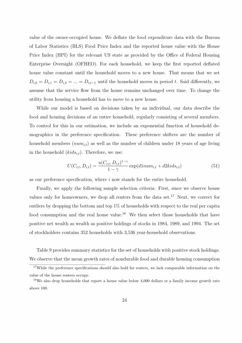
value of the owner-occupied house. We deflate the food expenditure data with the Bureau

of Labor Statistics (BLS) Food Price Index and the reported house value with the House

Price Index (HPI) for the relevant US state as provided by the Office of Federal Housing

Enterprise Oversight (OFHEO). For each household, we keep the first reported deflated

house value constant until the household moves to a new house. That means that we set

Di,0 = Di,1 = Di,2 = ... = Di,t−1 until the household moves in period t. Said differently, we

assume that the service flow from the house remains unchanged over time. To change the

utility from housing a household has to move to a new house.

While our model is based on decisions taken by an individual, our data describe the

food and housing decisions of an entire household, regularly consisting of several members.

To control for this in our estimation, we include an exponential function of household de-

mographics in the preference specification. These preference shifters are the number of

household members (numi,t) as well as the number of children under 18 years of age living

in the household (kidsi,t). Therefore, we use:

U(Ci,t, Di,t) =u(Ci,t, Di,t)

1−γ

1− γexp(d1numi,t + d2kidsi,t) (51)

as our preference specification, where i now stands for the entire household.

Finally, we apply the following sample selection criteria: First, since we observe house

values only for homeowners, we drop all renters from the data set.17 Next, we correct for

outliers by dropping the bottom and top 1% of households with respect to the real per capita

food consumption and the real house value.18 We then select those households that have

positive net wealth as wealth as positive holdings of stocks in 1984, 1989, and 1994. The set

of stockholders contains 352 households with 3,536 year-household observations.

Table 9 provides summary statistics for the set of households with positive stock holdings.

We observe that the mean growth rates of nondurable food and durable housing consumption

17While the preference specifications should also hold for renters, we lack comparable information on the

value of the house renters occupy.18We also drop households that report a house value below 4,000 dollars or a family income growth rate

above 100.

24

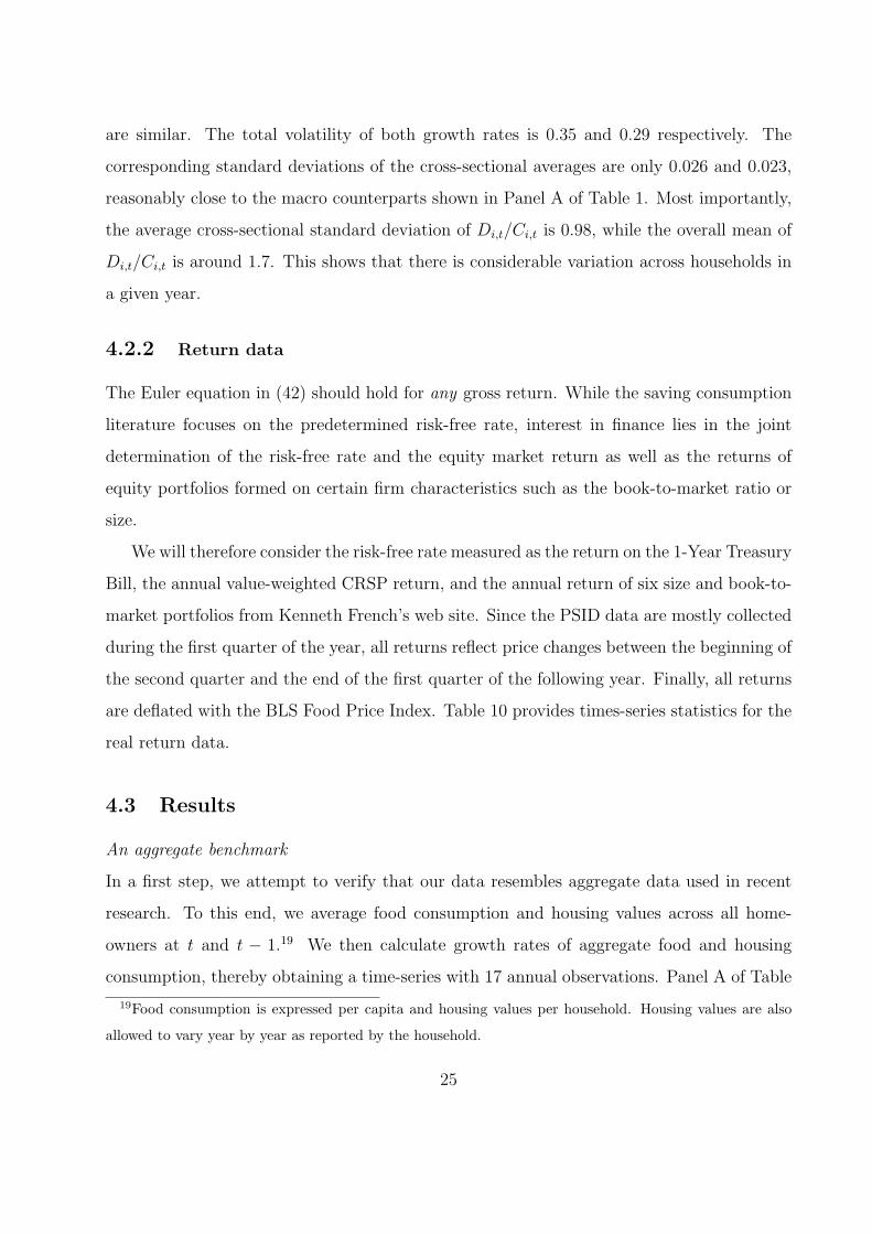
are similar. The total volatility of both growth rates is 0.35 and 0.29 respectively. The

corresponding standard deviations of the cross-sectional averages are only 0.026 and 0.023,

reasonably close to the macro counterparts shown in Panel A of Table 1. Most importantly,

the average cross-sectional standard deviation of Di,t/Ci,t is 0.98, while the overall mean of

Di,t/Ci,t is around 1.7. This shows that there is considerable variation across households in

a given year.

4.2.2 Return data

The Euler equation in (42) should hold for any gross return. While the saving consumption

literature focuses on the predetermined risk-free rate, interest in finance lies in the joint

determination of the risk-free rate and the equity market return as well as the returns of

equity portfolios formed on certain firm characteristics such as the book-to-market ratio or

size.

We will therefore consider the risk-free rate measured as the return on the 1-Year Treasury

Bill, the annual value-weighted CRSP return, and the annual return of six size and book-to-

market portfolios from Kenneth French’s web site. Since the PSID data are mostly collected

during the first quarter of the year, all returns reflect price changes between the beginning of

the second quarter and the end of the first quarter of the following year. Finally, all returns

are deflated with the BLS Food Price Index. Table 10 provides times-series statistics for the

real return data.

4.3 Results

An aggregate benchmark

In a first step, we attempt to verify that our data resembles aggregate data used in recent

research. To this end, we average food consumption and housing values across all home-

owners at t and t − 1.19 We then calculate growth rates of aggregate food and housing

consumption, thereby obtaining a time-series with 17 annual observations. Panel A of Table

19Food consumption is expressed per capita and housing values per household. Housing values are also

allowed to vary year by year as reported by the household.

25

11 reports statistics for this aggregate time series. Notice that the standard deviations of the

two annual consumption growth rates, 0.018 for food and 0.015 for housing consumption,

are slightly below the standard deviations of the annual aggregate data set (see Table 1 for

the summary statistics ). Panel B of Table 11 reports GMM estimates for the case of CES

and Cobb-Douglas preferences and Panel C reports GMM estimates for the linear approxi-

mation of those preferences. The test assets are the risk-free rate and the six Fama-French

portfolios. While noisy, the estimates appear in line with our own findings above and those

of Yogo (2006), who reports estimates of γ around 200.

We now turn to the main results of this section of the paper, the estimation of the Euler

equation on household-level data as described in Section 4.1. Unlike the GMM estimation

results reported so far, we will report only 1-step results, as 2-step GMM is often infeasible

when more than one test asset is used.20 We report two versions of Hansen’s overidentifi-

cation test: J-test (1) is based on raw model errors, while J-test (2) is based on demeaned

model errors. Finally, all standard errors are robust to heteroscedasticity and correlation

across households in a given year as well as to autocorrelation (for each unit and across

units) of up to two years.21

CES pricing kernel

Table 12 contains the estimation results when preferences are of the CES form. The in-

strument set includes household specific, state-specific, as well as macroeconomic variables.

In particular we use the following nine instruments: a constant, food consumption growth

(lagged twice), the ratio of housing over food consumption (lagged twice), income growth

(lagged twice), a dummy variable that is one if the household expects to move in the near

future (lagged twice), the change in the number of household members and in the number of

children under 18 years of age living in the household, the state unemployment rate (lagged

once), and the risk-free rate (lagged once).

20When both 1-step and 2-step GMM are feasible, results are very similar.21We use Newey-West (1987) weights in the construction of the covariance matrix.

26

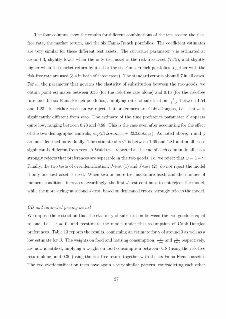
The four columns show the results for different combinations of the test assets: the risk-

free rate, the market return, and the six Fama-French portfolios. The coefficient estimates

are very similar for these different test assets. The curvature parameter γ is estimated at

around 3, slightly lower when the only test asset is the risk-free asset (2.75), and slightly

higher when the market return by itself or the six Fama-French portfolios together with the

risk-free rate are used (3.4 in both of those cases). The standard error is about 0.7 in all cases.

For ω, the parameter that governs the elasticity of substitution between the two goods, we

obtain point estimates between 0.35 (for the risk-free rate alone) and 0.18 (for the risk-free

rate and the six Fama-French portfolios), implying rates of substitution, 11−ω

, between 1.54

and 1.23. In neither case can we reject that preferences are Cobb-Douglas, i.e. that ω is

significantly different from zero. The estimate of the time preference parameter β appears

quite low, ranging between 0.73 and 0.88. This is the case even after accounting for the effect

of the two demographic controls, exp(d1∆numt+1 + d2∆kidst+1). As noted above, α and φ

are not identified individually. The estimate of αφω is between 1.66 and 1.81 and in all cases

significantly different from zero. A Wald test, reported at the end of each column, in all cases

strongly rejects that preferences are separable in the two goods, i.e. we reject that ω = 1−γ.

Finally, the two tests of overidentification, J-test (1) and J-test (2), do not reject the model

if only one test asset is used. When two or more test assets are used, and the number of

moment conditions increases accordingly, the first J-test continues to not reject the model,

while the more stringent second J-test, based on demeaned errors, strongly rejects the model.

CD and linearized pricing kernel

We impose the restriction that the elasticity of substitution between the two goods is equal

to one, i.e. ω = 0, and reestimate the model under this assumption of Cobb-Douglas

preferences. Table 13 reports the results, confirming an estimate for γ of around 3 as well as a

low estimate for β. The weights on food and housing consumption, 11+α

and α1+α

respectively,

are now identified, implying a weight on food consumption between 0.18 (using the risk-free

return alone) and 0.30 (using the risk-free return together with the six Fama-French assets).

The two overidentification tests have again a very similar pattern, contradicting each other

27

in the case of more than one test asset.

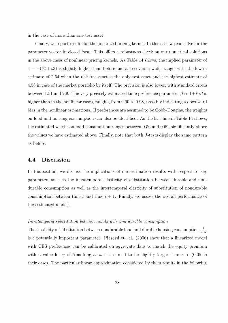
Finally, we report results for the linearized pricing kernel. In this case we can solve for the

parameter vector in closed form. This offers a robustness check on our numerical solutions

in the above cases of nonlinear pricing kernels. As Table 14 shows, the implied parameter of

γ = −(b2 + b3) is slightly higher than before and also covers a wider range, with the lowest

estimate of 2.64 when the risk-free asset is the only test asset and the highest estimate of

4.58 in case of the market portfolio by itself. The precision is also lower, with standard errors

between 1.51 and 2.9. The very precisely estimated time preference parameter β ≈ 1+ lnβ is

higher than in the nonlinear cases, ranging from 0.90 to 0.98, possibly indicating a downward

bias in the nonlinear estimations. If preferences are assumed to be Cobb-Douglas, the weights

on food and housing consumption can also be identified. As the last line in Table 14 shows,

the estimated weight on food consumption ranges between 0.56 and 0.69, significantly above

the values we have estimated above. Finally, note that both J-tests display the same pattern

as before.

4.4 Discussion

In this section, we discuss the implications of our estimation results with respect to key

parameters such as the intratemporal elasticity of substitution between durable and non-

durable consumption as well as the intertemporal elasticity of substitution of nondurable

consumption between time t and time t + 1. Finally, we assess the overall performance of

the estimated models.

Intratemporal substitution between nondurable and durable consumption

The elasticity of substitution between nondurable food and durable housing consumption 11−ω

is a potentially important parameter. Piazessi et. al. (2006) show that a linearized model

with CES preferences can be calibrated on aggregate data to match the equity premium

with a value for γ of 5 as long as ω is assumed to be slightly larger than zero (0.05 in

their case). The particular linear approximation considered by them results in the following

28

pricing kernel:

Mt+1 ≈ β

(1− γ∆lnCt+1 − γ + ω − 1

ω∆ln%t+1

)(52)

where %t+1 is the nondurable expenditure share as defined in (41). Our point estimates of

ω (see Table 12) fall between 0.18 and 0.35, far above the 0.05 assumed by Piazzesi et. al.

(2006). Given the size of the standard errors, however, we cannot reject that ω is equal to

0.05. Also, our micro data estimates are close to the estimates from a cointegration analysis

on aggregate nondurable and durable expenditure performed by Ogaki and Reinhart (1998),

but above the results from our own cointegration analysis in Section 3. Ogaki and Reinhart

(1998) estimate ω to be 0.19, while our own estimates from quarterly aggregate data (see

Table 3 Panel B) are -1.13 and -0.25.22

These results are very different, though, from the value for ω reported by Flavin and

Nakagawa (2004). They estimate the Euler equation implied by CES preferences over food

and housing consumption on PSID data, but estimate ω to be -6.5 with a standard error of

1.8. Comparing their results with our results is difficult, however, as their sample period is

shorter and they do not control for liquidity constraints and stock-ownership. Also different

from our approach, they measure the amount of housing consumption by using the estimated

size (in sq. ft.) of the household’s residence.

Our results confirm that even if adjustment costs are present, the elasticity of substi-

tution between nondurable and durable consumption can be estimated consistently from

aggregate data as long as cointegration analysis is used, because, as argued above, the two

consumption goods and relative user costs cannot evolve independently from each other in

the long run.

Intertemporal substitution

The EIS with respect to nondurable consumption is given by:

− UCi,t

Ci,tUCCi,t

=1 + αφω

(Di,t

Ci,t

)ω

γ − αφω(

Di,t

Ci,t

)ω

(ω − 1)(53)

22Remember that the coefficient estimate for the log of the relative price is 1ω−1 .

29

In the absence of adjustment costs, the ratioDi,t

Ci,twill be the same for all households, implying

that at each point in time the EIS will be the same across households. The economy-wide

EIS will change over time to the degree that the relative user cost for the service flow from

the durable good changes. In an economy with non-convex adjustment costs, the EIS will be

different across households as they differ in the ratioDi,t

Ci,t. For each household, the EIS will

change as this ratio changes unless ω = 0 (the Cobb-Douglas case) or ω = 1 − γ (the case

of separable preferences). If γ > 1, the EIS will decrease inDi,t

Ci,tas long as ω is in (1− γ, 0),

otherwise the EIS will increase asDi,t

Ci,tincreases. The economy-wide EIS will therefore depend

on the cross-sectional distribution of the ratioDi,t

Ci,tat any time.

Taking the medianDi,t

Ci,tof 1.52 and our estimates of ω (0.285), αφω (1.81), and γ (3.01)

from Table 12, the implied EIS is 0.68. Notice that this is about twice the value of the EIS

implied by the same value for γ if preferences were separable and of the CRRA form.

The equity premium and HJ-bounds

Our results suggest that estimation of the Euler equation using micro-level data leads to

reasonable parameter values, especially a low value for γ. Different from existing research on

asset pricing models using micro-level data, we incorporate durable consumption in the form

of consumption of housing services and find strong evidence that preferences are not separa-

ble. In this sense, we present a more comprehensive preference specification, consistent with

the renewed interest in two factor models as well as with the presence of adjustment costs.

At the same time, the overidentification tests cast some doubt on the overall performance of

the model.

In order to understand if the pricing kernel suggested in (42) can provide an answer to the

equity premium puzzle, we need to gain a better understanding of its time-series properties.

With only 17 years of annual observations, this is difficult in our setting. Nevertheless, we

evaluate the “aggregate” pricing kernel implied by our model (see (42)):

Mt+1 =1

N

N∑i=1

EtβUCi,t+1

UCi,t

(54)

Hansen and Jagannathan (1991) show that for any valid pricing kernel M , the following

30

inequality has to hold for any excess return Re:

σ(M)

E(M)≥ | E(Re) |

σ(Re)(55)

That is, the Hansen-Jagannathan (HJ) bound, the left-hand side of the inequality, has to

be at least as large as the Sharpe ratio of any asset. For our sample of all stockholders,

the time-series standard deviation of M is 0.11 and the mean is 0.90, implying a Hansen-

Jagannathan (HJ) bound of 0.12. While this value is above the HJ-bound of 0.09 implied

by parameter estimates in Jacobs (1999)23, it is still below the Sharpe ratio of the market

excess return, which is about 0.5. As we decrease ω, the HJ-bound decreases as well. When

ω = 0.1, for example, the implied HJ-bound is 0.08. On the other hand, when we increase

ω, the HJ-bound increases (for ω = 0.6, for example, the point estimate increases to 0.277).

These results show that additional tests of the model using a longer time series dimension

will be valuable.

5 Conclusions

A number of recent papers have tested the asset pricing implications of non-separable pref-

erences over nondurable and durable consumption. These papers assume that a frictionless

rental market for the durable good exists and that a representative agent can be constructed

so that tests can be carried out on aggregate data. We have tested one important implication

of these assumptions, namely that the ratio of aggregate marginal utilities equals the relative

user cost period by period. Our evidence strongly rejects this implication of the frictionless

model, while it is consistent with the presence of non-convex adjustment costs. Asset pricing

results based on aggregate data are affected by this finding and have to be re-evaluated in

the light of the evidence presented here.

Since aggregation in the traditional sense breaks down, we use micro-level data to test

the Euler equation for nondurable consumption. Thereby, we effectively average marginal

23We use the coefficient estimates from Panel A of Table III in Jacobs (1999) and apply them to our data

set.

31

utility growth across households. Our estimation results imply an elasticity of substitution

between food and housing consumption of around 1.40, with a standard error of 0.44 so

that we cannot rule out Cobb-Douglas preferences. Our results also imply a value for the

intertemporal elasticity of substitution (0.68) that is significantly higher than values derived

from aggregate data. At the same time, however, we find that the variability of our implied

aggregate pricing kernel is still too low to be reconciled with the observed US equity premium.

32

References

Ang, Andrew and Geert Bekaert, 2005, Stock Return Predictability: Is it There?, Review ofFinancial Studies, forthcoming.

Attanasio, Orazio P., 2000, Consumer Durables and Inertial Behavior: Estimation and Aggre-gation of (S,s) Rules for Automobile Purchases, Review of Economic Studies 67, 667-696.

Balduzzi, Pierluigi and Tong Yao, 2001, Testing heterogeneous-agent models: an alternativeaggregation approach, Journal of Monetary Economics 54, 369412.

Bar-Ilan, Avner and Alan L. Blinder, 1988, Consumer Durables and the Optimality of UsuallyDoing Nothing, NBER Working Paper.

Beaulieu, Joseph J., 1992, On Durable and Nondurable Consumption with Transactions Costs,MIT Dissertation, MIT.

Brav, Alon, George Constantinides, and Christopher Geczy, 2002, Asset Pricing with Het-erogeneous Consumers and Limited Participation: Empirical Evidence, Journal of PoliticalEconomy 110, 793-824.

Brennan, Michael J. and Alan Kraus, 1978, Necessary Conditions for Aggregation in SecurityMarkets, Journal of Financial and Quantitative Analysis 13, 407-418.

Bureau of Economic Analysis (BEA), 1990, Personal Consumption Expenditures, MethodologyPapers: US National Income and Product Accounts.

Caballero, Ricardo J., 1993, Durable Goods: An Explanation of Their Slow Adjustment, Jour-nal of Political Economy 101, 351-384.

Caballero, Ricardo J., 1994, Small Sample Bias and Adjustment Costs, Review of Economicsand Statistics 76, 52-58.

Carroll, Christopher D. and Wendy E. Dunn, 1997, Unemployment Expectations, Jumping(S,s) Triggers, and Household Balance Sheets, NBER Macroeconomics Annual, 1997.

Chamberlain, Garry, 1984, Panel Data; in Z. Griliches and M. Intriligator, eds.: Handbook ofEconometrics, Vol. 2 (North-Holland, Amsterdam).

Cogley, Timothy, 2002, Idiosyncratic Risk and the Equity Premium: Evidence from the Con-sumer Expenditure Survey, Journal of Monetary Economics 49, 309-334.

Damgaard, Anders, Brian Fuglsbjerg, and Claus Munk, 2003, Optimal Consumption and Invest-ment Strategies with a Perishable and an Indivisible Durable Consumption Good, Journalof Economic Dynamics & Control 28, 209-253.

Detemple, Jerome B. and Christos I. Giannikos, 1996, Asset and Commodity Prices with Multi-Attribute Durable Goods, Journal of Economic Dynamics and Control 20, 1451-1504.

Dunn, Kenneth B. and Kenneth J. Singleton, 1986, Modeling the Term Structure of InterestRates under Nonseparable Utility and Durability of Goods, Journal of Financial Economics41, 333-355.

Eberly, Janice C., 1994, Adjustment of Consumers’ Durable Stocks: Evidence from Automobile

33

Purchases, Journal of Political Economy 102, 403-436.

Eichenbaum, Martin and Lars Peter Hansen, 1990, Estimating Models with Intertemporal Sub-stitution Using Aggregate Times Series Data, Journal of Business and Economic Statistics8, 53-69.

Flavin, Majorie and Shinobu Nakagawa, 2004, A Model of Housing in the Presence of Adjust-ment Costs: A Structural Interpretation of Habit Persistence, NBER Working Paper.

Grossman, Sanford J. and Guy Laroque, 1990, Asset Pricing and Optimal Portfolio Choice inthe Presence of Illiquid Durable Consumption Goods, Econometrica 58, 25-52.

Hansen, Lars Peter, 1982, Large Sample Properties of Generalized Method of Moments Esti-mators, Econometrica 50, 1029-1054.

Hansen, Lars Peter and Ravi Jagannathan, 1991, Implications of Security Market Data forModels of Dynamic Economies, Journal of Political Economy 99, 225-262.

Hayashi, Fumio, 1985, The Permanent Income Hypothesis and Consumption Durability: Anal-ysis on Japanese Panel Data, Quarterly Journal of Economics 100, 1083-1113.

Jacobs, Kris, 1999, Incomplete Markets and Security Prices: Do Asset-Pricing Puzzles Resultfrom Aggregation Problems?, Journal of Finance 54, 123-163.

Jacobs, Kris and Kevin Q. Wang, 2004, Idiosyncratic Consumption Risk and the Cross-Sectionof Asset Returns, Journal of Finance 59, 2211-2252.

Kullmann, Cornelia and Stephan Siegel, 2005, Real Estate and its Role in Household PortfolioChoice, Working Paper, UBC.

Lustig, Hanno N. and Stijn G. Van Nieuwerburgh, 2005, Housing Collateral, ConsumptionInsurance, and Risk Premia: An Empirical Perspective, Journal of Finance 60, 11671219.

Mamaysky, Harry, 2001, Interest Rates and the Durability of Consumption Goods, WorkingPaper, Yale School of Management.

Mankiw, N. Gregory and Stephen P. Zeldes 1990, The Consumption of Stockholders and Non-Stockholders, NBER Working Paper.

Marshall, David A. and Nayan G. Parekh, 1999, Can Costs of Consumption Adjustment ExplainAsset Pricing Puzzles, Journal of Finance 54, 623-654.

Martin, Robert F., 2001, Consumption, Durable Goods, and Transaction Costs, Working Paper,University of Chicago.

Newey, Whitney and Kenneth West, 1987, A simple positive semi-definite, heteroscedasticityand autocorrelation consistent covariance matrix, Econometrica 55, 703-708.

Murray, Jonathan and Nicholas Sarantis, 1999, Quality, User Cost, Forward Looking Behavior,and the Demand for Cars in the UK, Journal of Economics and Business 51, 237-258.

Ogaki, Masao and Carmen M. Reinhart, 1998, Measuring Intertemporal Substitution: The Roleof Durable Goods, Journal of Political Economy 106, 1078-1098.

34

Padula, Mario, 1999, Euler Equations and Durable Goods, Working Paper, Centre for Studiesin Economics and Finance.

Pakos, Michal, 2003, Asset Pricing with Durable Goods and Non-Homothetic Preferences,Working Paper, University of Chicago.

Park, Joon Y., 1992, Canonical Cointegration Regressions, Econometrica 60, 119-143.

Parker, Jonathan A. and Christian Julliard, 2005, Consumption Risk and the Cross Section ofExpected Returns, Journal of Political Economy 113, 185222.

Piazzesi, Monika, Martin Schneider, and Selale Tuzel, 2003, Housing, Consumption, and AssetPricing, Journal of Financial Economics,forthcoming.

Rubinstein, Mark, 1974, An Aggregation Theorem for Securities Markets, Journal of FinancialEconomics 1, 225-244.

Stock, James H. and Mark W. Watson, 1993, A Simple Estimator of Cointegrating Vectors inHigher Order Integrated Systems, Econometrica 61, 783-820.

Vissing-Jørgensen, Annette, 2002, Limited Asset Market Participation and the Elasticity ofIntertemporal Substitution, Journal of Political Economy 110, 825-853.

Yogo, Motohiro, 2006, A Consumption-Based Explanation of Expected Stock Returns, Journalof Finance 61, 539580.

Zeldes, Stephen P., 1989, Consumption and Liquidity Constraints: An Empirical Investigation,Journal of Political Economy 97, 305-346.

35

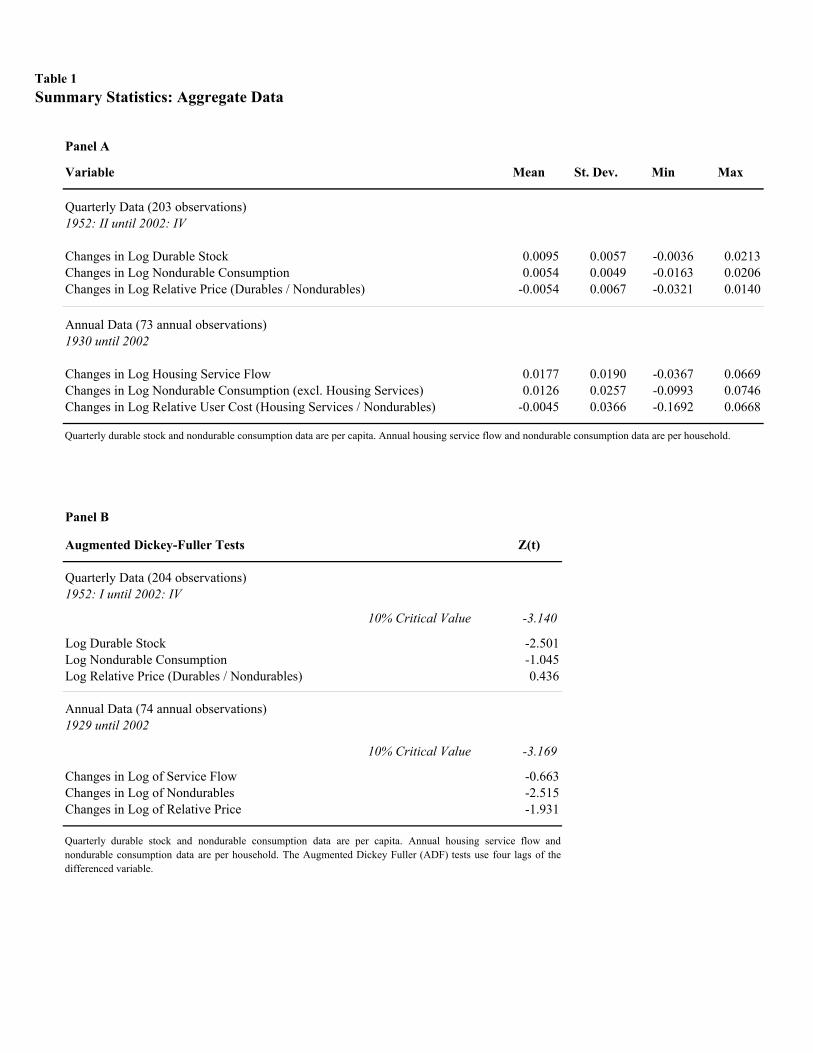
Table 1Summary Statistics: Aggregate Data

Panel A

Variable Mean St. Dev. Min Max

Quarterly Data (203 observations)1952: II until 2002: IV

Changes in Log Durable Stock 0.0095 0.0057 -0.0036 0.0213Changes in Log Nondurable Consumption 0.0054 0.0049 -0.0163 0.0206Changes in Log Relative Price (Durables / Nondurables) -0.0054 0.0067 -0.0321 0.0140

Annual Data (73 annual observations)1930 until 2002

Changes in Log Housing Service Flow 0.0177 0.0190 -0.0367 0.0669Changes in Log Nondurable Consumption (excl. Housing Services) 0.0126 0.0257 -0.0993 0.0746Changes in Log Relative User Cost (Housing Services / Nondurables) -0.0045 0.0366 -0.1692 0.0668

Panel B

Augmented Dickey-Fuller Tests Z(t)

Quarterly Data (204 observations)1952: I until 2002: IV

10% Critical Value -3.140

Log Durable Stock -2.501Log Nondurable Consumption -1.045Log Relative Price (Durables / Nondurables) 0.436

Annual Data (74 annual observations)1929 until 2002

10% Critical Value -3.169

Changes in Log of Service Flow -0.663Changes in Log of Nondurables -2.515Changes in Log of Relative Price -1.931

Quarterly durable stock and nondurable consumption data are per capita. Annual housing service flow and nondurable consumption data are per household.

Quarterly durable stock and nondurable consumption data are per capita. Annual housing service flow andnondurable consumption data are per household. The Augmented Dickey Fuller (ADF) tests use four lags of thedifferenced variable.

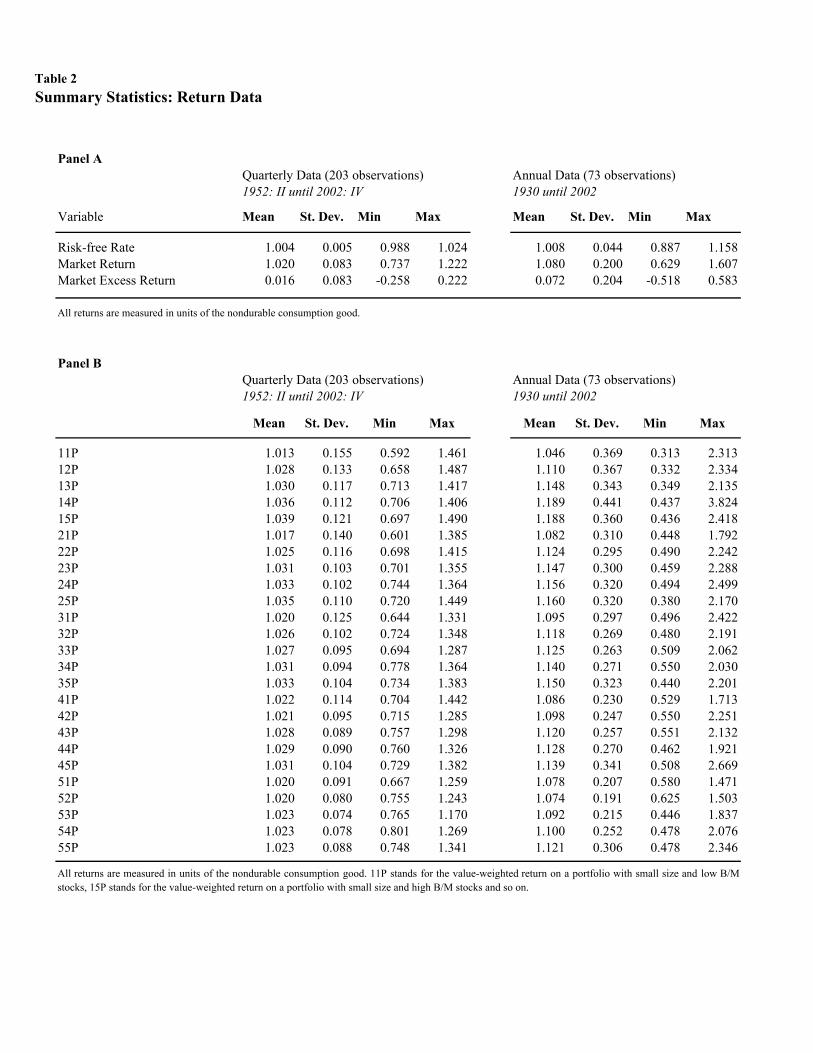
Table 2Summary Statistics: Return Data

Panel AQuarterly Data (203 observations) Annual Data (73 observations)1952: II until 2002: IV 1930 until 2002

Variable Mean St. Dev. Min Max Mean St. Dev. Min Max

Risk-free Rate 1.004 0.005 0.988 1.024 1.008 0.044 0.887 1.158Market Return 1.020 0.083 0.737 1.222 1.080 0.200 0.629 1.607Market Excess Return 0.016 0.083 -0.258 0.222 0.072 0.204 -0.518 0.583

Panel BQuarterly Data (203 observations) Annual Data (73 observations)1952: II until 2002: IV 1930 until 2002

Mean St. Dev. Min Max Mean St. Dev. Min Max

11P 1.013 0.155 0.592 1.461 1.046 0.369 0.313 2.31312P 1.028 0.133 0.658 1.487 1.110 0.367 0.332 2.33413P 1.030 0.117 0.713 1.417 1.148 0.343 0.349 2.13514P 1.036 0.112 0.706 1.406 1.189 0.441 0.437 3.82415P 1.039 0.121 0.697 1.490 1.188 0.360 0.436 2.41821P 1.017 0.140 0.601 1.385 1.082 0.310 0.448 1.79222P 1.025 0.116 0.698 1.415 1.124 0.295 0.490 2.24223P 1.031 0.103 0.701 1.355 1.147 0.300 0.459 2.28824P 1.033 0.102 0.744 1.364 1.156 0.320 0.494 2.49925P 1.035 0.110 0.720 1.449 1.160 0.320 0.380 2.17031P 1.020 0.125 0.644 1.331 1.095 0.297 0.496 2.42232P 1.026 0.102 0.724 1.348 1.118 0.269 0.480 2.19133P 1.027 0.095 0.694 1.287 1.125 0.263 0.509 2.06234P 1.031 0.094 0.778 1.364 1.140 0.271 0.550 2.03035P 1.033 0.104 0.734 1.383 1.150 0.323 0.440 2.20141P 1.022 0.114 0.704 1.442 1.086 0.230 0.529 1.71342P 1.021 0.095 0.715 1.285 1.098 0.247 0.550 2.25143P 1.028 0.089 0.757 1.298 1.120 0.257 0.551 2.13244P 1.029 0.090 0.760 1.326 1.128 0.270 0.462 1.92145P 1.031 0.104 0.729 1.382 1.139 0.341 0.508 2.66951P 1.020 0.091 0.667 1.259 1.078 0.207 0.580 1.47152P 1.020 0.080 0.755 1.243 1.074 0.191 0.625 1.50353P 1.023 0.074 0.765 1.170 1.092 0.215 0.446 1.83754P 1.023 0.078 0.801 1.269 1.100 0.252 0.478 2.07655P 1.023 0.088 0.748 1.341 1.121 0.306 0.478 2.346

All returns are measured in units of the nondurable consumption good. 11P stands for the value-weighted return on a portfolio with small size and low B/Mstocks, 15P stands for the value-weighted return on a portfolio with small size and high B/M stocks and so on.

All returns are measured in units of the nondurable consumption good.

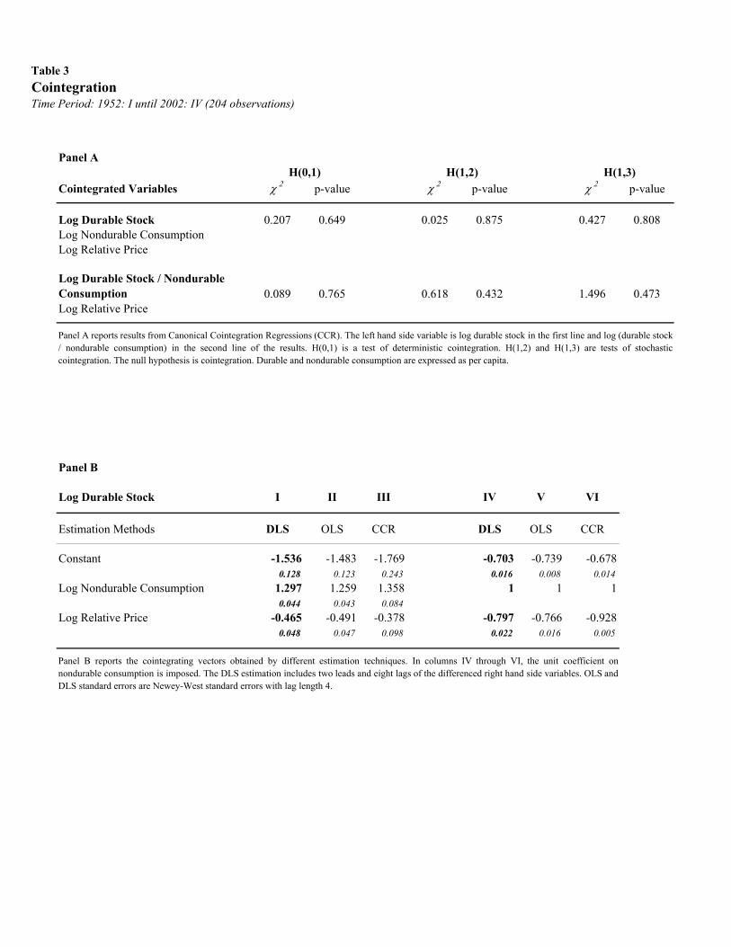
Table 3Cointegration Time Period: 1952: I until 2002: IV (204 observations)

Panel A

Cointegrated Variables χ 2 p-value χ 2 p-value χ 2 p-value

Log Durable Stock 0.207 0.649 0.025 0.875 0.427 0.808Log Nondurable ConsumptionLog Relative Price

Log Durable Stock / Nondurable Consumption 0.089 0.765 0.618 0.432 1.496 0.473Log Relative Price

Panel B

Log Durable Stock I II III IV V VI

Estimation Methods DLS OLS CCR DLS OLS CCR

Constant -1.536 -1.483 -1.769 -0.703 -0.739 -0.6780.128 0.123 0.243 0.016 0.008 0.014

Log Nondurable Consumption 1.297 1.259 1.358 1 1 10.044 0.043 0.084

Log Relative Price -0.465 -0.491 -0.378 -0.797 -0.766 -0.9280.048 0.047 0.098 0.022 0.016 0.005

Panel B reports the cointegrating vectors obtained by different estimation techniques. In columns IV through VI, the unit coefficient onnondurable consumption is imposed. The DLS estimation includes two leads and eight lags of the differenced right hand side variables. OLS andDLS standard errors are Newey-West standard errors with lag length 4.

H(0,1) H(1,3)H(1,2)

Panel A reports results from Canonical Cointegration Regressions (CCR). The left hand side variable is log durable stock in the first line and log (durable stock/ nondurable consumption) in the second line of the results. H(0,1) is a test of deterministic cointegration. H(1,2) and H(1,3) are tests of stochasticcointegration. The null hypothesis is cointegration. Durable and nondurable consumption are expressed as per capita.

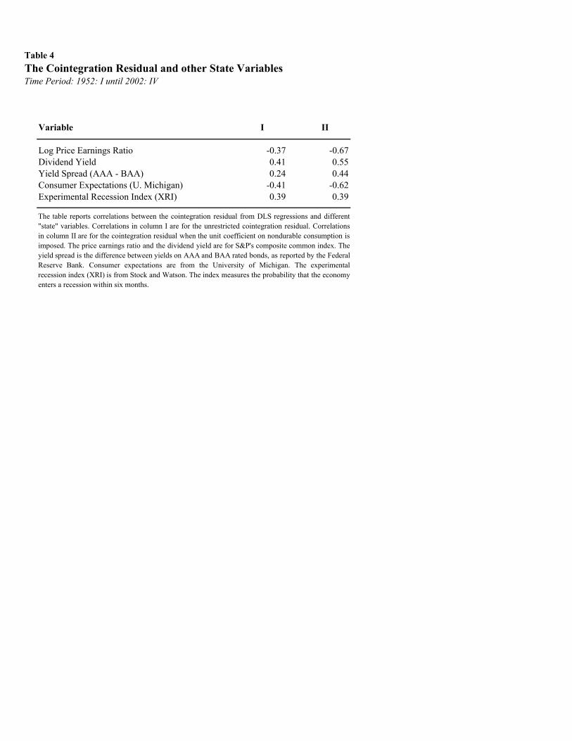
Table 4The Cointegration Residual and other State VariablesTime Period: 1952: I until 2002: IV

Variable I II

Log Price Earnings Ratio -0.37 -0.67Dividend Yield 0.41 0.55Yield Spread (AAA - BAA) 0.24 0.44Consumer Expectations (U. Michigan) -0.41 -0.62Experimental Recession Index (XRI) 0.39 0.39

The table reports correlations between the cointegration residual from DLS regressions and different"state" variables. Correlations in column I are for the unrestricted cointegration residual. Correlationsin column II are for the cointegration residual when the unit coefficient on nondurable consumption isimposed. The price earnings ratio and the dividend yield are for S&P's composite common index. Theyield spread is the difference between yields on AAA and BAA rated bonds, as reported by the FederalReserve Bank. Consumer expectations are from the University of Michigan. The experimentalrecession index (XRI) is from Stock and Watson. The index measures the probability that the economyenters a recession within six months.

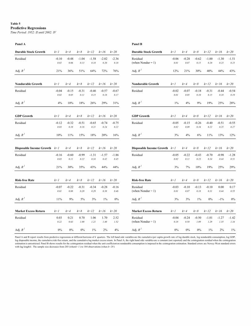
Table 5Predictive RegressionsTime Period: 1952: II until 2002: IV

Panel A Panel B

Durable Stock Growth k=1 k=4 k=8 k=12 k=16 k=20 Durable Stock Growth k=1 k=4 k=8 k=12 k=16 k=20

Residual -0.10 -0.48 -1.04 -1.58 -2.02 -2.36 Residual -0.06 -0.28 -0.62 -1.00 -1.30 -1.510.02 0.06 0.13 0.18 0.20 0.18 (when Nondur = 1) 0.01 0.07 0.15 0.20 0.23 0.25

Adj. R 2 21% 36% 51% 64% 72% 76% Adj. R 2 12% 21% 30% 40% 44% 43%

Nondurable Growth k=1 k=4 k=8 k=12 k=16 k=20 Nondurable Growth k=1 k=4 k=8 k=12 k=16 k=20

Residual -0.04 -0.15 -0.31 -0.46 -0.57 -0.67 Residual -0.02 -0.07 -0.18 -0.31 -0.44 -0.540.02 0.05 0.11 0.15 0.18 0.17 0.01 0.05 0.10 0.15 0.18 0.19

Adj. R 2 4% 10% 18% 26% 29% 31% Adj. R 2 1% 4% 9% 19% 25% 28%

GDP Growth k=1 k=4 k=8 k=12 k=16 k=20 GDP Growth k=1 k=4 k=8 k=12 k=16 k=20

Residual -0.12 -0.32 -0.51 -0.65 -0.74 -0.75 Residual -0.05 -0.15 -0.26 -0.40 -0.51 -0.550.03 0.10 0.16 0.21 0.24 0.22 0.02 0.09 0.16 0.22 0.25 0.27

Adj. R 2 10% 11% 15% 18% 20% 16% Adj. R 2 3% 4% 6% 11% 13% 12%

Disposable Income Growth k=1 k=4 k=8 k=12 k=16 k=20 Disposable Income Growth k=1 k=4 k=8 k=12 k=16 k=20

Residual -0.16 -0.60 -0.99 -1.31 -1.57 -1.86 Residual -0.05 -0.22 -0.43 -0.70 -0.98 -1.280.03 0.11 0.22 0.34 0.42 0.45 0.02 0.11 0.23 0.34 0.44 0.51

Adj. R 2 21% 30% 35% 43% 44% 44% Adj. R 2 3% 7% 10% 19% 25% 29%

Risk-free Rate k=1 k=4 k=8 k=12 k=16 k=20 Risk-free Rate k=1 k=4 k=8 k=12 k=16 k=20

Residual -0.07 -0.22 -0.31 -0.34 -0.28 -0.16 Residual -0.03 -0.10 -0.13 -0.10 0.00 0.170.01 0.08 0.20 0.29 0.38 0.46 (when Nondur = 1) 0.01 0.07 0.18 0.31 0.44 0.55

Adj. R 2 11% 9% 5% 3% 1% 0% Adj. R 2 3% 3% 1% 0% -1% 0%

Market Excess Return k=1 k=4 k=8 k=12 k=16 k=20 Market Excess Return k=1 k=4 k=8 k=12 k=16 k=20

Residual 0.03 0.21 0.70 1.06 1.70 2.52 Residual -0.04 -0.24 -0.50 -1.01 -1.27 -1.420.22 0.63 1.00 1.21 1.40 1.52 (when Nondur = 1) 0.18 0.58 1.09 1.29 1.35 1.34

Adj. R 2 0% 0% 0% 1% 2% 4% Adj. R 2 0% 0% 0% 1% 2% 1%

Panel A and B report results from predictive regressions at different horizons of k quarters. The left hand side variables are the cumulative per capita growth rate of log durable stock, log nondurable consumption, log GDP,log disposable income, the cumulative risk-free return, and the cumulative log market excess return. In Panel A, the right hand side variables are a constant (not reported) and the cointegration residual when the cointegrationestimation is unrestricted. Panel B shows results for the cointegration residual when the unit coefficient on nondurable consumption is imposed in the cointegration estimation. Standard errors are Newey-West standard errorswith lag length k . The sample size decreases from 203 (when k=1 ) to 184 observations (when k=20 )

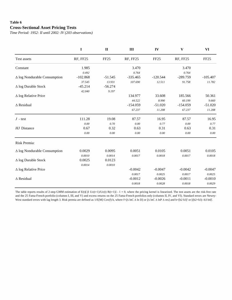
Table 6 Cross-Sectional Asset Pricing TestsTime Period: 1952: II until 2002: IV (203 observations)

I II III IV V VI

Test assets RF, FF25 FF25 RF, FF25 FF25 RF, FF25 FF25

Constant 1.985 3.470 3.4700.492 0.764 0.764

Δ log Nondurable Consumption -102.868 -51.545 -335.465 -120.544 -289.759 -105.40737.545 13.931 107.690 12.511 91.758 11.782

Δ log Durable Stock -45.214 -56.27442.040 9.197

Δ log Relative Price 134.977 33.608 185.566 50.36144.522 8.990 60.199 9.660

Δ Residual -154.059 -51.020 -154.059 -51.02067.237 11.208 67.237 11.208

J - test 111.28 19.08 87.57 16.95 87.57 16.950.00 0.70 0.00 0.77 0.00 0.77

HJ Distance 0.67 0.32 0.63 0.31 0.63 0.310.00 0.00 0.00 0.00 0.00 0.00

Risk Premia:

Δ log Nondurable Consumption 0.0029 0.0095 0.0051 0.0105 0.0051 0.01050.0010 0.0014 0.0017 0.0018 0.0017 0.0018

Δ log Durable Stock 0.0025 0.01230.0014 0.0010

Δ log Relative Price -0.0042 -0.0047 -0.0042 -0.00470.0017 0.0025 0.0017 0.0025

Δ Residual -0.0012 -0.0026 -0.0011 -0.00100.0018 0.0028 0.0018 0.0029

The table reports results of 2-step GMM estimation of E(t)[ β Uc(t+1)/Uc(t) R(t+1)] - 1 = 0, where the pricing kernel is linearized. The test assets are the risk-free rateand the 25 Fama-French portfolio (columns I, III, and V) and excess returns on the 25 Fama-French portfolios only (columns II, IV, and VI). Standard errors are Newey-West standard errors with lag length 3. Risk premia are defined as 1/E[M] Cov(f) b, where f=[Δ lnC Δ ln D] or [Δ lnC Δ lnP Δ res] and b=[b2 b3]' or [(b2+b3) -b3 b4]'.

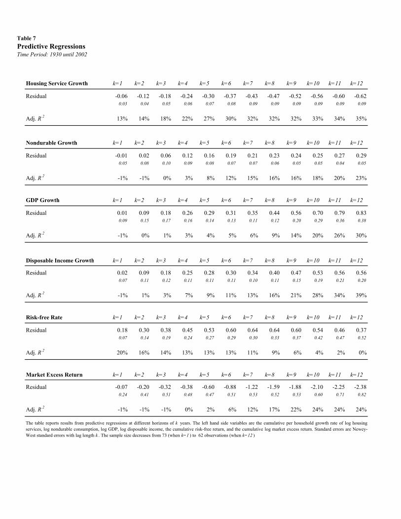
Table 7Predictive RegressionsTime Period: 1930 until 2002

Housing Service Growth k=1 k=2 k=3 k=4 k=5 k=6 k=7 k=8 k=9 k=10 k=11 k=12

Residual -0.06 -0.12 -0.18 -0.24 -0.30 -0.37 -0.43 -0.47 -0.52 -0.56 -0.60 -0.620.03 0.04 0.05 0.06 0.07 0.08 0.09 0.09 0.09 0.09 0.09 0.09

Adj. R 2 13% 14% 18% 22% 27% 30% 32% 32% 32% 33% 34% 35%

Nondurable Growth k=1 k=2 k=3 k=4 k=5 k=6 k=7 k=8 k=9 k=10 k=11 k=12

Residual -0.01 0.02 0.06 0.12 0.16 0.19 0.21 0.23 0.24 0.25 0.27 0.290.05 0.08 0.10 0.09 0.08 0.07 0.07 0.06 0.05 0.05 0.04 0.05

Adj. R 2 -1% -1% 0% 3% 8% 12% 15% 16% 16% 18% 20% 23%

GDP Growth k=1 k=2 k=3 k=4 k=5 k=6 k=7 k=8 k=9 k=10 k=11 k=12

Residual 0.01 0.09 0.18 0.26 0.29 0.31 0.35 0.44 0.56 0.70 0.79 0.830.09 0.15 0.17 0.16 0.14 0.13 0.11 0.12 0.20 0.29 0.36 0.38

Adj. R 2 -1% 0% 1% 3% 4% 5% 6% 9% 14% 20% 26% 30%

Disposable Income Growth k=1 k=2 k=3 k=4 k=5 k=6 k=7 k=8 k=9 k=10 k=11 k=12

Residual 0.02 0.09 0.18 0.25 0.28 0.30 0.34 0.40 0.47 0.53 0.56 0.560.07 0.11 0.12 0.11 0.11 0.11 0.10 0.11 0.15 0.19 0.21 0.20

Adj. R 2 -1% 1% 3% 7% 9% 11% 13% 16% 21% 28% 34% 39%

Risk-free Rate k=1 k=2 k=3 k=4 k=5 k=6 k=7 k=8 k=9 k=10 k=11 k=12

Residual 0.18 0.30 0.38 0.45 0.53 0.60 0.64 0.64 0.60 0.54 0.46 0.370.07 0.14 0.19 0.24 0.27 0.29 0.30 0.33 0.37 0.42 0.47 0.52

Adj. R 2 20% 16% 14% 13% 13% 13% 11% 9% 6% 4% 2% 0%

Market Excess Return k=1 k=2 k=3 k=4 k=5 k=6 k=7 k=8 k=9 k=10 k=11 k=12

Residual -0.07 -0.20 -0.32 -0.38 -0.60 -0.88 -1.22 -1.59 -1.88 -2.10 -2.25 -2.380.24 0.41 0.51 0.48 0.47 0.51 0.53 0.52 0.53 0.60 0.71 0.82

Adj. R 2 -1% -1% -1% 0% 2% 6% 12% 17% 22% 24% 24% 24%

The table reports results from predictive regressions at different horizons of k years. The left hand side variables are the cumulative per household growth rate of log housingservices, log nondurable consumption, log GDP, log disposable income, the cumulative risk-free return, and the cumulative log market excess return. Standard errors are Newey-West standard errors with lag length k . The sample size decreases from 73 (when k=1 ) to 62 observations (when k=12 )

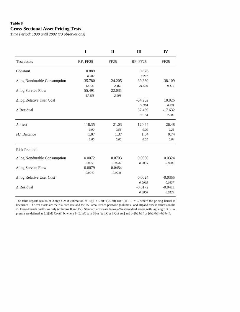
Table 8Cross-Sectional Asset Pricing TestsTime Period: 1930 until 2002 (73 observations)

I II III IV

Test assets RF, FF25 FF25 RF, FF25 FF25

Constant 0.889 0.8760.282 0.291

Δ log Nondurable Consumption -35.780 -24.205 39.380 -38.10912.733 2.465 21.569 9.113

Δ log Service Flow 55.491 -22.03117.858 2.998

Δ log Relative User Cost -34.252 18.82614.364 6.831

Δ Residual 57.439 -17.63218.164 7.885

J - test 118.35 21.03 120.44 26.480.00 0.58 0.00 0.23

HJ Distance 1.07 1.37 1.04 0.740.00 0.00 0.01 0.04

Risk Premia:

Δ log Nondurable Consumption 0.0072 0.0703 0.0080 0.03240.0055 0.0047 0.0055 0.0080

Δ log Service Flow -0.0079 0.04540.0042 0.0031

Δ log Relative User Cost 0.0024 -0.03550.0065 0.0137

Δ Residual -0.0172 -0.04110.0068 0.0124

The table reports results of 2-step GMM estimation of E(t)[ b Uc(t+1)/Uc(t) R(t+1)] - 1 = 0, where the pricing kernel islinearized. The test assets are the risk-free rate and the 25 Fama-French portfolio (columns I and III) and excess returns on the25 Fama-French portfolios only (columns II and IV). Standard errors are Newey-West standard errors with lag length 3. Riskpremia are defined as 1/E[M] Cov(f) b, where f=[Δ lnC Δ ln S] or [Δ lnC Δ lnQ Δ res] and b=[b2 b3]' or [(b2+b3) -b3 b4]'.

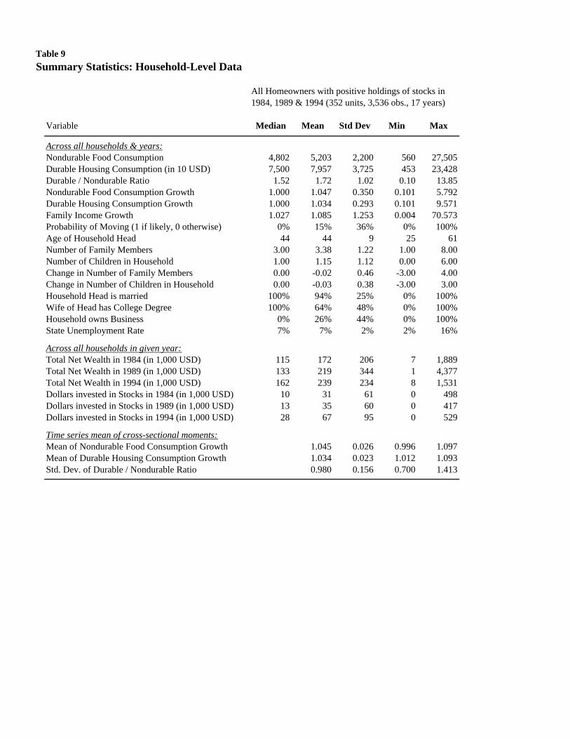
Table 9Summary Statistics: Household-Level Data

All Homeowners with positive holdings of stocks in 1984, 1989 & 1994 (352 units, 3,536 obs., 17 years)

Variable Median Mean Std Dev Min Max

Across all households & years:Nondurable Food Consumption 4,802 5,203 2,200 560 27,505Durable Housing Consumption (in 10 USD) 7,500 7,957 3,725 453 23,428Durable / Nondurable Ratio 1.52 1.72 1.02 0.10 13.85Nondurable Food Consumption Growth 1.000 1.047 0.350 0.101 5.792Durable Housing Consumption Growth 1.000 1.034 0.293 0.101 9.571Family Income Growth 1.027 1.085 1.253 0.004 70.573Probability of Moving (1 if likely, 0 otherwise) 0% 15% 36% 0% 100%Age of Household Head 44 44 9 25 61Number of Family Members 3.00 3.38 1.22 1.00 8.00Number of Children in Household 1.00 1.15 1.12 0.00 6.00Change in Number of Family Members 0.00 -0.02 0.46 -3.00 4.00Change in Number of Children in Household 0.00 -0.03 0.38 -3.00 3.00Household Head is married 100% 94% 25% 0% 100%Wife of Head has College Degree 100% 64% 48% 0% 100%Household owns Business 0% 26% 44% 0% 100%State Unemployment Rate 7% 7% 2% 2% 16%

Across all households in given year:Total Net Wealth in 1984 (in 1,000 USD) 115 172 206 7 1,889Total Net Wealth in 1989 (in 1,000 USD) 133 219 344 1 4,377Total Net Wealth in 1994 (in 1,000 USD) 162 239 234 8 1,531Dollars invested in Stocks in 1984 (in 1,000 USD) 10 31 61 0 498Dollars invested in Stocks in 1989 (in 1,000 USD) 13 35 60 0 417Dollars invested in Stocks in 1994 (in 1,000 USD) 28 67 95 0 529

Time series mean of cross-sectional moments:Mean of Nondurable Food Consumption Growth 1.045 0.026 0.996 1.097Mean of Durable Housing Consumption Growth 1.034 0.023 1.012 1.093Std. Dev. of Durable / Nondurable Ratio 0.980 0.156 0.700 1.413

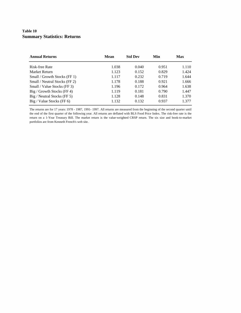
Table 10Summary Statistics: Returns

Annual Returns Mean Std Dev Min Max

Risk-free Rate 1.038 0.040 0.951 1.110Market Return 1.123 0.152 0.829 1.424Small / Growth Stocks (FF 1) 1.117 0.232 0.719 1.644Small / Neutral Stocks (FF 2) 1.178 0.188 0.921 1.666Small / Value Stocks (FF 3) 1.196 0.172 0.964 1.638Big / Growth Stocks (FF 4) 1.119 0.181 0.790 1.447Big / Neutral Stocks (FF 5) 1.128 0.148 0.831 1.370Big / Value Stocks (FF 6) 1.132 0.132 0.937 1.377

The returns are for 17 years: 1978 - 1987, 1991- 1997. All returns are measured from the beginning of the second quarter untilthe end of the first quarter of the following year. All returns are deflated with BLS Food Price Index. The risk-free rate is thereturn on a 1-Year Treasury Bill. The market return is the value-weighted CRSP return. The six size and book-to-marketportfolios are from Kenneth French's web site.

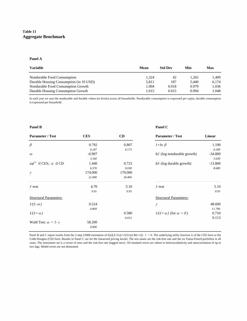
Table 11Aggregate Benchmark

Panel A

Variable Mean Std Dev Min Max

Nondurable Food Consumption 1,324 42 1,265 1,409Durable Housing Consumption (in 10 USD) 5,811 187 5,440 6,174Nondurable Food Consumption Growth 1.004 0.018 0.979 1.036Durable Housing Consumption Growth 1.015 0.015 0.994 1.048

Panel B Panel C

Parameter / Test CES CD Parameter / Test Linear

β 0.792 0.807 1+ln β 1.1900.187 0.173 0.189

ω -0.907 b2 (log nondurable growth) -34.8003.160 3.630

αφ ω if CES; α if CD 1.440 0.723 b3 (log durable growth) -13.8006.570 0.038 8.680

γ 174.000 179.00021.000 18.400

J -test 4.70 5.10 J -test 5.100.91 0.93 0.93

Structural Parameters: Structural Parameters:

1/(1-ω ) 0.524 γ 48.6000.869 11.700

1/(1+α ) 0.580 1/(1+α ) (for ω = 0 ) 0.7100.013 0.113

Wald Test: ω = 1- γ 58.2000.000

In each year we sum the nondurable and durable values (in levels) across all households. Nondurable consumption is expressed per capita, durable consumptionis expressed per household.

Panel B and C report results from the 2-step GMM estimation of E(t)[ β Uc(t+1)/Uc(t) R(t+1)] - 1 = 0. The underlying utility function is of the CES form or theCobb-Douglas (CD) form. Results in Panel C are for the linearized pricing kernel. The test assets are the risk-free rate and the six Fama-French portfolios in allcases. The instrument set is a vector of ones and the risk-free rate (lagged once). All standard errors are robust to heteroscedasticity and autocorrelation of up totwo lags. Model errors are not demeaned.

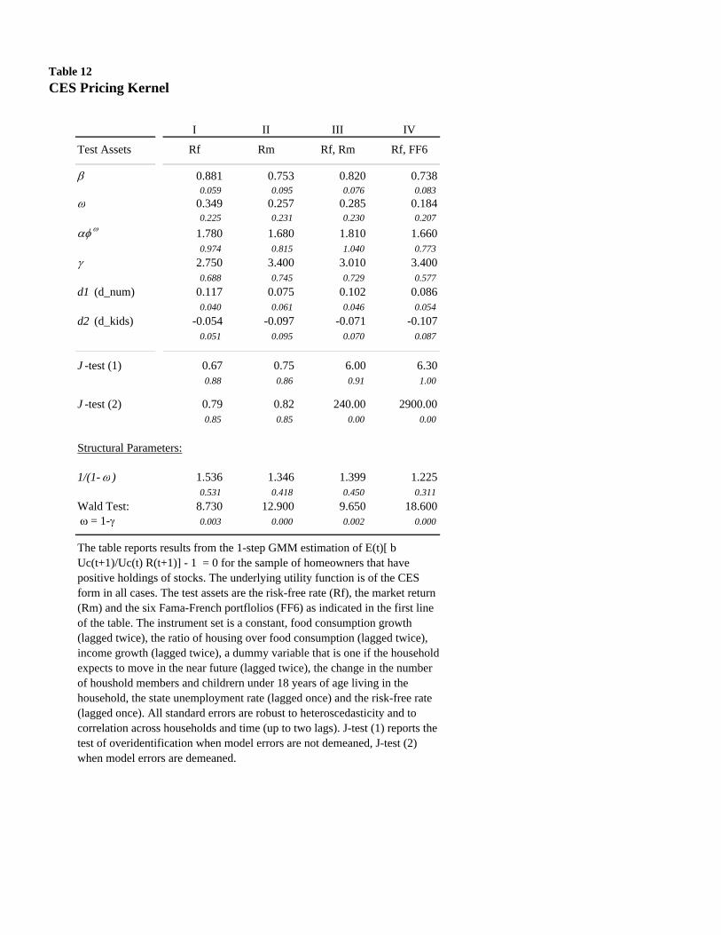
Table 12CES Pricing Kernel

I II III IV

Test Assets Rf Rm Rf, Rm Rf, FF6

β 0.881 0.753 0.820 0.7380.059 0.095 0.076 0.083

ω 0.349 0.257 0.285 0.1840.225 0.231 0.230 0.207

αφ ω 1.780 1.680 1.810 1.6600.974 0.815 1.040 0.773

γ 2.750 3.400 3.010 3.4000.688 0.745 0.729 0.577

d1 (d_num) 0.117 0.075 0.102 0.0860.040 0.061 0.046 0.054

d2 (d_kids) -0.054 -0.097 -0.071 -0.1070.051 0.095 0.070 0.087

J -test (1) 0.67 0.75 6.00 6.300.88 0.86 0.91 1.00

J -test (2) 0.79 0.82 240.00 2900.000.85 0.85 0.00 0.00

Structural Parameters:

1/(1-ω ) 1.536 1.346 1.399 1.2250.531 0.418 0.450 0.311

Wald Test: 8.730 12.900 9.650 18.600 ω = 1-γ 0.003 0.000 0.002 0.000

The table reports results from the 1-step GMM estimation of E(t)[ b Uc(t+1)/Uc(t) R(t+1)] - 1 = 0 for the sample of homeowners that have positive holdings of stocks. The underlying utility function is of the CES form in all cases. The test assets are the risk-free rate (Rf), the market return (Rm) and the six Fama-French portflolios (FF6) as indicated in the first line of the table. The instrument set is a constant, food consumption growth (lagged twice), the ratio of housing over food consumption (lagged twice), income growth (lagged twice), a dummy variable that is one if the household expects to move in the near future (lagged twice), the change in the number of houshold members and childrern under 18 years of age living in the household, the state unemployment rate (lagged once) and the risk-free rate (lagged once). All standard errors are robust to heteroscedasticity and to correlation across households and time (up to two lags). J-test (1) reports the test of overidentification when model errors are not demeaned, J-test (2) when model errors are demeaned.

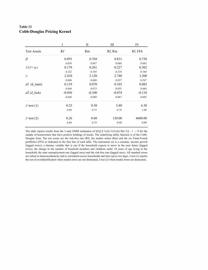
Table 13Cobb-Douglas Pricing Kernel

I II III IV

Test Assets Rf Rm Rf, Rm Rf, FF6

β 0.893 0.769 0.831 0.7500.050 0.087 0.068 0.083

1/(1+α ) 0.179 0.261 0.227 0.3020.232 0.195 0.218 0.168

γ 2.410 3.120 2.740 3.2000.606 0.680 0.657 0.567

d1 (d_num) 0.119 0.070 0.103 0.0850.046 0.073 0.055 0.068

d2 (d_kids) -0.056 -0.100 -0.074 -0.1100.048 0.089 0.067 0.083

J -test (1) 0.25 0.58 5.80 6.300.88 0.75 0.76 1.00

J -test (2) 0.26 0.60 120.00 4600.000.88 0.74 0.00 0.00

The table reports results from the 1-step GMM estimation of E(t)[ β Uc(t+1)/Uc(t) R(t+1)] - 1 = 0 for thesample of homeowners that have positive holdings of stocks. The underlying utility function is of the Cobb-Douglas form. The test assets are the risk-free rate (Rf), the market return (Rm) and the six Fama-Frenchportflolios (FF6) as indicated in the first line of each table. The instrument set is a constant, income growth(lagged twice), a dummy variable that is one if the household expects to move in the near future (laggedtwice), the change in the number of houshold members and childrern under 18 years of age living in thehousehold, the state unemployment rate (lagged once) and the risk-free rate (lagged once). All standard errorsare robust to heteroscedasticity and to correlation across households and time (up to two lags). J-test (1) reports the test of overidentification when model errors are not demeaned, J-test (2) when model errors are demeaned.

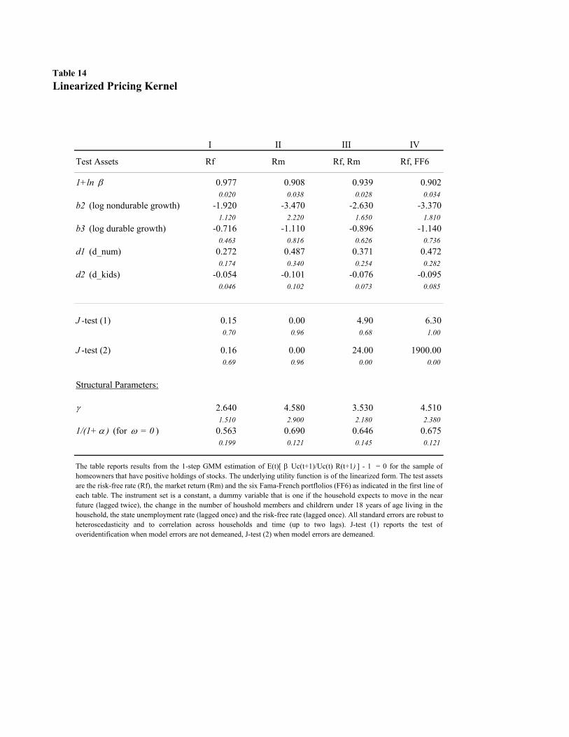
Table 14Linearized Pricing Kernel

I II III IV

Test Assets Rf Rm Rf, Rm Rf, FF6

1+ln β 0.977 0.908 0.939 0.9020.020 0.038 0.028 0.034

b2 (log nondurable growth) -1.920 -3.470 -2.630 -3.3701.120 2.220 1.650 1.810

b3 (log durable growth) -0.716 -1.110 -0.896 -1.1400.463 0.816 0.626 0.736

d1 (d_num) 0.272 0.487 0.371 0.4720.174 0.340 0.254 0.282

d2 (d_kids) -0.054 -0.101 -0.076 -0.0950.046 0.102 0.073 0.085

J -test (1) 0.15 0.00 4.90 6.300.70 0.96 0.68 1.00

J -test (2) 0.16 0.00 24.00 1900.000.69 0.96 0.00 0.00

Structural Parameters:

γ 2.640 4.580 3.530 4.5101.510 2.900 2.180 2.380

1/(1+α ) (for ω = 0 ) 0.563 0.690 0.646 0.6750.199 0.121 0.145 0.121

The table reports results from the 1-step GMM estimation of E(t)[ β Uc(t+1)/Uc(t) R(t+1) ] - 1 = 0 for the sample ofhomeowners that have positive holdings of stocks. The underlying utility function is of the linearized form. The test assetsare the risk-free rate (Rf), the market return (Rm) and the six Fama-French portflolios (FF6) as indicated in the first line ofeach table. The instrument set is a constant, a dummy variable that is one if the household expects to move in the nearfuture (lagged twice), the change in the number of houshold members and childrern under 18 years of age living in thehousehold, the state unemployment rate (lagged once) and the risk-free rate (lagged once). All standard errors are robust toheteroscedasticity and to correlation across households and time (up to two lags). J-test (1) reports the test ofoveridentification when model errors are not demeaned, J-test (2) when model errors are demeaned.

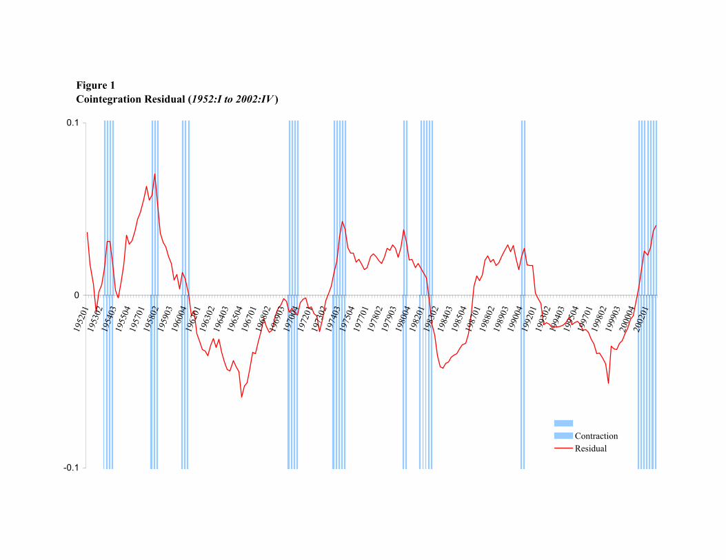
Figure 1 Cointegration Residual (1952:I to 2002:IV )

-0.1

0

0.1

195201

195302

195403

195504

195701

195802

195903

196004

196201

196302

196403

196504

196701

196802

196903

197004

197201

197302

197403

197504

197701

197802

197903

198004

198201

198302

198403

198504

198701

198802

198903

199004

199201

199302

199403

199504

199701

199802

199903

200004

200201

ContractionResidual