Using Data-Driven Domain Randomization to Transfer Robust ControlPolicies to Mobile Robots

Matthew Sheckells1, Gowtham Garimella1, Subhransu Mishra1, and Marin Kobilarov1

Abstract— This work develops a technique for using robotmotion trajectories to create a high quality stochastic dy-namics model that is then leveraged in simulation to traincontrol policies with associated performance guarantees. Wedemonstrate the idea by collecting dynamics data from a 1/5scale agile ground vehicle, fitting a stochastic dynamics model,and training a policy in simulation to drive around an ovaltrack at up to 7 m/s while avoiding obstacles. We show thatthe control policy can be transferred back to the real vehiclewith little loss in predicted performance. We compare this toan approach that uses a simple analytic car model to traina policy in simulation and show that using a model withstochasticity learned from data leads to higher performance interms of trajectory tracking accuracy and collision probability.Furthermore, we show that simulation-derived performanceguarantees transfer to the actual vehicle when executing a policyoptimized using a stochastic dynamics model fit to vehicle data.

I. INTRODUCTION

Training control policies for a robotic system in simulationis attractive since data can be generated quickly and thesafety of the robot is not a concern. However, policies trainedin simulation often do not perform as well when transferredto the real world since the simulator may not completelymatch reality. Recent research suggests that domain random-ization is a promising approach to generating policies that arerobust to modelling errors in the simulator [1], [2], [3], [4],[5]. This technique injects noise into the model parametersor dynamics of the simulated system in order to make thegenerated control policy reliable under a variety of condi-tions. Many procedures, however, choose the uncertainty ofthe simulator in an ad-hoc, hand-tuned manner, often withgreat results [2], [3].

In this work, we propose to learn the uncertainty of thesimulator in a data-driven fashion. We first fit a stochasticdynamics model to data generated from the real system.Then, we use this model to train a control policy usingthe stochastic dynamics. We train the policy using PROPS,a reinforcement learning algorithm that searches in policyspace and which uses the training data to generate a sta-tistical performance guarantee for future executions of thepolicy [6]. We show that when the policy is transferred tothe real robot that the performance guarantees computed insimulation, such as not exceeding a given probability ofcollision, still hold. An important consequence of this is that

1M. Sheckells, G. Garimella, S. Mishra, and M. Kobi-larov are with the Department of Computer Science andthe Department of Mechanical Engineering, Johns HopkinsUniversity, 3400 N Charles Str, Baltimore, MD 21218, USAmsheckells|ggarime1|smishra9|marin@jhu.edu

Fig. 1. The JHU all-terrain mobile robot used for navigation experiments.

we can approximately quantify and improve the expectedperformance and safety of a policy in simulation beforeexecuting it on the actual physical system. We demonstratethis approach by computing an obstacle avoiding trajectorytracking control policy for an agile Unmanned GroundVehicle (UGV) travelling up to 7 m/s. We show that thisapproach outperforms a relatively simple procedure whichtrains a policy in simulation using a simple analytic model.

A. Related Work

This work is closely related to recent research in usingdomain randomization in reinforcement learning as well asolder developments in nonlinear system identification andmodel-based policy search.

1) Domain Randomization: Using domain randomizationto make control policies robust to the transfer from simu-lation to reality, also known as “sim-to-real”, is a relativelynew avenue of research that has seen a lot of activity over thelast two years. Tobin et al. first used domain randomizationin a rendering engine to train an object detector completelyin simulation and then use it in the real world to performrobotic grasping [1]. Researchers at OpenAI similarly trainedan object pose estimation model in simulation using arandomized renderer while also using reinforcement learningto optimize a control strategy for in-hand manipulation in arandomized simulation. They were able to transfer both thepose estimator and control strategy to a real robotic handwith little performance degradation [2]. Other work trainedcontrol policies in simulation with randomized dynamics andsuccessfully deployed the policies on real robots for pushingobjects [4] and quadruped control [3], Sadeghi et al. traineda visual servoing policy in simulation while randomizing

properties such as camera viewpoint and lighting conditions,showing that the transferred policy generalized to unseenobjects in the real world [5].

2) Stochastic Dynamics Modelling: Neural networks area powerful tool for modelling nonlinear functions, so re-searchers have used them to model nonlinear system dy-namics [7], [8], [9] and stochastic dynamics [10] for the pasttwo decades. A different approach is to use Gaussian Process(GP) regression [11] or Bayesian neural networks [12], [13]to model the dynamics and covariance as a continuousfunction of the state and control input.

3) Model-based Policy Search: This work falls in therealm of model-based policy search since we fit a modelof the system using data from the vehicle and leverage thatfor stochastic policy optimization. There are several relatedworks: PILCO learns a stochastic dynamics model usinga GP and explicitly incorporates uncertainty into planningand control while using approximate inference to evaluatethe policy and an analytic policy gradient to make policyupdates [14]. Kupcsik et al. leverage a model of the dynamicsfor contextual policy learning, adapting a low level policyto the situation at hand [15]. Guided policy search fits aseries of linear-Gaussian models to local system dynamics,while using a Gaussian Mixture Model to capture a roughglobal estimate of the dynamics. These models are usedto optimize local policies which are then used as targetdistributions for fitting a global policy [16]. More recentwork used Bayesian neural networks to model a stochasticnonlinear system and leveraged the model for stochasticpolicy optimization [17]. Rajeswaran et al. developed theEPOpt algorithm which uses adversarial training and anensemble of simulated source domains to train a policythat is robust to different target domains and unmodelleddisturbances. Furthermore, EPOpt can leverage data fromthe target domain and use Bayesian methods to make thesimulated domain a better approximation of the target [18].The proposed approach is similar to related work in that itfinds a maximum likelihood estimate of the target system andthen uses it for policy optimization in simulation. The keydifference here is that we show empirically that performanceguarantees generated by the PROPS policy search algorithmtransfer to the real system when using a learned stochasticmodel.

II. DATA-DRIVEN DOMAIN RANDOMIZATION

Policy transfer from simulation to a real robot often leadsto suboptimal or even unsafe results if the policy is trainedin a single, deterministic environment. This is because smalldifferences between the simulated and real environment canlead to drastic differences in policy behavior. Recent researchhas shown that randomizing some aspects of the environmentrobustifies the policy and leads to better policy transfer.This technique is called domain randomization. Here, weintroduce a procedure for modelling the uncertainty in thereal environment in order to inject uncertainty into thesimulation. Previous techniques use an ad-hoc procedureto pick which parameters of the simulation to randomize.

This usually leads to a tuning procedure in which there isa trade-off between policy robustness and how conservativethe policy is, where more noise leads to a more robust yetmore conservative policy. In contrast to this, we attempt tolearn the dynamics distribution from robot-generated data sothat the policy is not overly conservative. Next, we describethe model and how we use it for generating random systemtrajectories.

A. Stochastic Dynamics Model

The state of the dynamic system is denoted by x ∈ Rnwith control inputs u ∈ Rm. We assume that the dynamicstake the form of a stochastic ODE

x = f(x, u) + g(x, u)w,

where w(t) is a random variable taking values in R` sampledfrom a standard Gaussian N (0, I`), uncorrelated in time. Thefunctions f and g are the mean and the Cholesky form ofthe covariance of the dynamics, respectively. More formally:

E[x(t)] = f(x(t), u(t)),

E[x(t)x(τ)T ] = g(x(t), u(t))g(x(t), u(t))>δ(t− τ),where δ(t − τ) is the Dirac delta for given times t and τ .While ` can be chosen high enough to capture the noisecomplexity, we set ` = n for the rest of this work as it workswell in practice without making the model too complex. Thedynamics can be approximated by some parameterized modelfθ and gγ . Next, we describe the loss function for fitting sucha model to dynamics data.

B. Model Loss Function

Given trajectory data from a real system, we can findfunctions fθ and gγ which maximize the likelihood of thedata and therefore provide a good probabilistic model of thesystem.

Assume that we have M samples of the dynamics X ={x1. . . . , xM}, U = {u1, . . . , uM}, X = {x1. . . . , xM}. Tosimplify notation, we denote fi , fθ(xi, ui) and gi ,gγ(xi, ui). The likelihood of the data is given by the jointprobability density

p(X|θ, γ,X,U) =

M∏i=1

e−12 (xi−fi)

>g−1>i g−1

i (xi−fi)√(2π)n|gig>i |

.

As is typical, we can instead maximize the simpler loglikelihood

ln p(X|θ, γ,X,U) =

M∑i=1

− 1

2(xi − fi)>g−1

>

i g−1i (xi − fi)

− 1

2ln |gig>i | −

n

2ln 2π.

Since g is lower triangular, the last two terms above can besimplified to −∑j ln gijj − n

2 ln 2π. Furthermore, g−1i (xi−fi) can be solved efficiently using forward substitution sincegi is lower triangular. Thus, we can fit a probabilistic modelof the dynamics by minimizing the loss

L(θ, γ) =M∑i=1

1

2(xi − fi)>g−1

>

i g−1i (xi − fi) +∑j

ln gijj .

Fig. 2. Neural networks used for modelling the system dynamics

C. Model Architecture

In this work, we choose fθ and gγ to be simple neuralnetworks. Both consist of an input layer, several fully-connected hidden layers with ReLU activation functions,and an output layer. The fθ network simply outputs an n-dimensional vector. The gγ network outputs n(n + 1)/2numbers that are re-shaped into a lower triangular matrix.The diagonal of the matrix is constrained to a positivenumber by exponentiating the diagonal output from gγ . Wethen add a small regularizing constant to the diagonal toensure invertibility of the matrix. We whiten the data beforepassing it to the input layer to normalize the data andavoid saturating activation functions. Each hidden layers usesbatch normalization also to avoid activation saturation. Thearchitecture is illustrated in Figure 2.

D. Sampling Trajectories from Stochastic Model

Starting from an initial state x0, we can generate a randomtrajectory sample using the stochastic model with an Eulerintegration scheme

xi+1 = xi + ˜x dt,

where dt is the simulation time step and ˜x is sampled fromN (fθ(xi, ui), gγ(xi, ui)gγ(xi, ui)

>). Thus, we can use thelearned stochastic model to randomize the environment whileperforming stochastic policy optimization.

III. STOCHASTIC POLICY OPTIMIZATION

With a good probabilistic model of the dynamics in hand,the goal of policy search is to find an optimal policy for themodel. Also of primary importance is providing a formalguarantee on the future performance of the system under thepolicy. In this section, we review a previously developed pol-icy search method that directly minimizes a bound on futureperformance, called PAC Robust Policy Search (PROPS) [6],with PAC meaning ”probably-approximately-correct”.

A common way to define policy search in policy parameterspace is through the optimization

ν∗ = argminν

Eτ,ξ∼p(·|ν)[J(τ)],

where J is a cost function encoding the desired behavior, ξis a vector of decision variables defining the control policy,

τ is the system response governed by the density p(·|ξ), andν parameterizes a surrogate distribution over the decisionvariables. The surrogate stochastic model induces a jointdensity p(τ, ξ|ν) = p(τ |ξ)π(ξ|ν) which contains the naturalstochasticity of the system p(τ |ξ) and artificial control-exploration stochasticity π(ξ|ν) due to the surrogate model.

PROPS works within the framework of Iterative StochasticPolicy Optimization (ISPO). The goal of ISPO is to generatean optimal control policy which minimizes the cost functionJ (ν) , E τ,ξ∼p(·|ν) [J(τ)]. We perform the search directlyin the parameter space of the policy and learn a distributionover the policy parameters π(·|ν). ISPO iteratively buildsa surrogate stochastic model π(ξ|ν) from which a policy ξcan be sampled. The goal is to then minimize the expectedcost J (ν) iteratively until convergence. This usually cor-responds to π(ξ|ν) shrinking to a tight peak around ξ∗ oraround several peaks if the distribution is multi-modal. Thegeneral framework for solving the problem is described inAlgorithm 1.

Algorithm 1 Iterative Stochastic Policy Optimization (ISPO)1: Initialize hyper-distribution ν0, i← 02: while Bound on expected cost greater than threshold do3: for j = 1, . . . ,M do4: Sample trajectory (ξj , τj) ∼ p(·|νi)5: Compute a new policy νi+1 using observed costs{J(τ1), . . . , J(τM )}, set i = i+ 1

A key step in ISPO is computing the new policy basedon the observed costs of previously executed policies. Thespecific implementation of the update step (Step 5) corre-sponds to different policy search algorithms such as Reward-weighted Regression (RwR) [19] or Relative Entropy PolicySearch (REPS) [20]. This work uses a recently introducedalgorithm called PAC Robust Policy Search (PROPS) forupdating the policy based on minimizing an upper confidencebound on its expected future cost. PROPS performs anoptimization of the form

minν,αJα(ν) + αd(ν, ν0) + φ(α,N, δ), (1)

where Jα is a robust empirical estimate of J , d(·, ·) denotesa distance between policy distributions, N is the number ofsamples, and φ is a concentration-of-measure term whichreflects the discrepancy between the empirical cost Jα andthe true mean cost J . The expression in (1) (denoted J +)is in fact a high-confidence bound on the expected cost, i.e.with probability 1 − δ it hold that J ≤ J +. PROPS isexplained in more detail in previous work [6].

IV. TRAINING OBSTACLE AVOIDANCE POLICY FOR ANAGILE MOBILE ROBOT

Using the procedure outlined in §II, we learn a stochasticdynamic model of a 1/5 scale off-road UGV and use itto train a control policy in simulation using the algorithmdescribed in §III. Furthermore, we train another controlpolicy on a simple kinematic car model using the same

0.0 1.8 3.7 5.5 7.0

Velocity (m/s)

-0.5

-0.2

0.0

0.3

0.5

Ste

eri

ng a

ngle

(ra

d)

Log Position Dynamics Covariance

-4.5

-3.0

-1.5

0.0

Fig. 3. Log position dynamics covariance (computed as log (σ2px

+ σ2py

))histogram over steering angle and velocity for the learned stochasticdynamics. The model learns that p is noisier at higher steering angles andvelocities. Here, the orientation input to the covariance model is θ = 0, butwe see similar results for all θ ∈ [−π, π]. Furthermore, to generate thishistogram we set vc = v, δc = δ.

policy search algorithm and compare the performance ofeach policy when evaluated on the real vehicle. The goalof each policy is to track an oval trajectory at a speed of7 m/s while avoiding randomly generated obstacles in thepath of the vehicle. Figure 4 illustrates the task.

A. Robot

Our UGV is a heavily modified 1/5 scale Redcat RacingRampage XB-E equipped with an onboard Gigabyte BRIXcomputer with an i7 processor. A LORD Microstrain 3DM-GX4-25 IMU measures inertial data while a u-blox C94-M8PRTK GPS computes global position. A hall effect sensorencoder measures the rotation rate of the drive shaft, which isconverted to the body velocity of the vehicle after calibration.

B. Stochastic Model

We collected about 30 minutes of dynamics data, includingposition, orientation, wheel velocity, steering angle, andsteering and velocity commands, while manually driving thecar on an astroturf field and took care to make sure thedata distribution evenly spanned the state-action space of thevehicle expected for the task. We built a stochastic dynamicsmodel using the technique described in §II, using 3 hiddenlayers of 64 units for both the f and g models. Figure 2illustrates the model, where the model inputs include the carorientation θ, body-x velocity v, steering angle δ, velocitycommand vc, and commanded steering angle δc. The modeloutputs x, with x = (p, θ, v, δ), where p = (px, py) ∈ R2 isthe position of the vehicle.

The learned mean dynamics of the car behaved similarlyto a simple kinematic car model at lower velocities, whilethe learned covariance model indicated higher noise in p athigher velocities and sharper steering angles as illustrated inFigure 3.

C. Control Policy

Using the model discussed in the previous section, weoptimize a control policy for the off-road vehicle in sim-ulation using PROPS. We use a policy based on feedback

controllers for achieving desired lateral offset, speed, andobstacle avoidance, with relatively few learnable parameters.Next, we discuss the representation of the car that we use forthe policy and then explain the details of the policy itself.

1) Curvilinear Car Dynamics: During motion planning, itis useful to express the state of an autonomous vehicle withrespect to some curvilinear coordinate system. For example,the reference curvature of the coordinate system can followthe center line of a road or path. We define the state of thevehicle as xcurv = (s, er, eθ, v, a, δ) ∈ R6, where s is thearc length along the reference path, er is the lateral offsetfrom the path, eθ is the angular offset from the path tangentat s, and v is the forward body-velocity, and a is the forwardbody-acceleration. The control inputs to the system consistof the jerk u1 ∈ R and steering angle rate u2 ∈ R. Typicalbicycle dynamics expressed using path coordinates are givenas

sereθva

δ

=

v cos eθ1−κ(s)erv sin eθ

v(tan δL − κ(s)s

)au1u2

, (2)

where κ(s) is the curvature of the path at s and L is thelength of the vehicle [21].

2) Controller Design: While there exists previous workwhich can perform obstacle avoidance while guiding thesystem to a static goal (e.g. [22], [23], [24]), to the author’sknowledge no such control design methodology exists tosimultaneously track a trajectory and avoid obstacles whileproviding convergence guarantees.

Here, we design a Lyapunov stable controller that achievesa desired track offset and velocity in a de-coupled manner.A higher level planner commands a track offset to the lateralcontroller that is computed to avoid any detected obstacles.

Lateral controller: The lateral controller guides thevehicle to the center of the track lane, i.e. er = 0. We derivesuch a control law using backstepping on the lateral offset.We start with the Lyapunov candidate V0 = 1

2krpe2r +

12 e

2r ,

which has the time derivativeV0 = er[krper + er]

= er

[krper + u1 sin eθ + v cos eθ

(θ − v κ(s) cos eθ

1− κ(s)er

)]with θ , v tan δ

L and krp > 0. Setting θ to the desired value

θd , vκ(s) cos eθ1− κ(s)er

+1

v cos eθ(−krper − a sin eθ − krd er)

with krd > 0 makes V0 ≤ 0 and renders the system stable,but we cannot directly set θ to θd. Thus, we create a secondstorage function V1 which drives the error zθ , θ − θd tozero

V1 = V0 +1

2z2θ .

Fig. 4. The robot using an optimized control policy to follow a 22 m × 14 m oval track at 6.5 m/s while avoiding virtual obstacles.

Noting that V0 = er[v cos eθ(θ − θd)]− krd e2r , we have

V1 = zθ[erv cos eθ + zθ]− krd e2r= zθ

[erv cos eθ +

a tan δ

L+v sec2 δ

Lδ − θd

]− krd e2r.

Setting

u2 = δ =L cos2 δ

v

[−a tan δ

L+ θd − erv cos eθ − kzθzθ

]makes V1 ≤ 0, thereby stabilizing the system. Thus, δ gives acontrol law for tracking a reference line and has three tunableparameters krp , krd , kzθ .

Speed Control: The speed control law is a simplePD controller on the forward-jerk u1 of the vehicle u1 =kvp(vd − v) − kvda to achieve a desired speed vd. Thedesired speed is set to the goal speed vgoal while the vehicleis driving straight; however, it is often important for thevehicle to slow down while turning to avoid obstacles. So, weintroduce a tunable lateral acceleration constraint alatmax,which limits vd to be smaller at larger steering angles, i.e.vd ≤ vmax(δ) ,

√alatmaxL/| tan δ|. If vgoal < vmax, we

set vd = vgoal.Obstacle Avoidance: A high level control strategy

chooses the desired track offset for the vehicle based onthe position of detected obstacles. If an obstacle is detectedwithin some radius of the vehicle, denoted kdet, then thedesired track offset is shifted by a distance kshift awayfrom the obstacle in the direction that the vehicle is pointingrelative to the obstacle. So, if the robot is pointing to the leftof the obstacle, then the desired track offset is shifted to theleft. If the track itself is already far enough away from thedetected obstacle, then no shift occurs. Both kdet and kshiftare tunable parameters in the navigation system.

Thus, the whole navigation policy has 8 tunable param-eters: lateral gains krp , krd , kzθ , velocity control parame-ters kvp , kvd , alatmax, and obstacle avoidance parameterskdet, kshift. These compose the vector ξ ∈ R8 (see Sec. III).

D. Policy Optimization

Navigation Cost: The policy search cost function thatwe attempt to minimize takes the form

J(τ)=

tf∑t=0

[Ra2t+Qrer2t+Qv(vt/vgoal−1)2 + |vt|O(dt)]dt,

where R,Qr, Qv > 0 are tuning weights, dt is the time step,and O(d) is a cost that encourages obstacle avoidance andis defined as

O(d) =

O(olow) + Clow(olow − d)2, d < olow

Chigh(ohigh − d)2, olow < d < ohigh

0, otherwise,

where d is the distance from the car to the closest obstaclewith distance measured from the edge of the car to the edgeof the obstacle. The variables ohigh and olow are distancethresholds that determine when the car incurs a small penaltyor a large penalty for being close to the obstacle, respectively.

For our experiments we set vgoal = 6.5m/s, tf = 7s, dt =0.02s, R = 10−3, Qr = 0.25, Qv = 4, Clow = 800, Chigh =80, olow = 0.5m, and ohigh = 1.0m.

Stochastic Policies: The surrogate policy p(·|ν) is aGaussian with a diagonal covariance matrix. We initializethe surrogate policy to have a standard deviation of 2 in alldimensions.

Environment: The robot attempts to follow a 22 m ×14 m oval track at a goal velocity of 6.5 m/s. At the start ofeach episode, an obstacle is randomly generated 8m in frontof the vehicle with a track offset uniformly distributed in therange [−4m, 4m] and a radius uniformly distributed in therange [0.3m, 1.0m]. An episode terminates either when therobot has hit an obstacle or when tf seconds have elapsed.When the episode terminates, the obstacle is cleared anda new obstacle is generated at the beginning of the nextepisode. The robot state at the end of one episode is thesame as its initial state at the beginning of the next episode,i.e. the robot remains in motion from one episode to the next.

Policy Search: We train each policy for 260 iterationsusing PROPS, collecting 50 episodes (i.e. trajectory roll-outs) in each iteration and using a sliding window of 20batches for each policy update. For the PROPS algorithm,we set the bound confidence 1 − δ = .95 indicating thatthe computed performance bound should hold with 95%probability. PROPS is not sensitive to this user-selectedparameter and has no other tunable parameters.

E. Results and Discussion

Figures 5 and 6 show the convergence of the navigationpolicy parameters and trajectory costs over time for the

2.5

5.0

kv p

4

6

kv d

2

4

kr p

2.5

5.0

kr d

10.0

12.5

kz θ

2.5

5.0

kdet

0 200

0.0

2.5

ksh

ift

0 200

2.5

5.0alatm

ax

Policy v.s. Iterations

0 50 100 150 200 250Iterations

10

20

30

40

50

Cost v.s. Iterations

J

J +

Fig. 5. Convergence of navigation policy (left) and cost (right) for policyoptimized using a stochastic model of the car learned from real-world data.

2.5

5.0

kv p

2.5

5.0kv d

2.55.0

kr p

2.5

5.0

kr d

8

10

12

kz θ

2.5

5.0

kdet

0 200

0

5

ksh

ift

0 200

2.5

5.0

alatm

ax

Policy v.s. Iterations

0 50 100 150 200 250Iterations

0

10

20

30

40

50

Cost v.s. Iterations

J

J +

Fig. 6. Convergence of navigation policy (left) and cost (right) for policyoptimized using a simple kinematic car model.

learned stochastic model and simple car model, respectively.The policy trained on the simple model learns to trackthe reference much more aggressively with a larger krpand smaller krd . It also computes a much larger obstacleavoidance distance kshift and smaller detection radius kdetcompared to the policy trained on the stochastic model.

Table I compares the average absolute track offset |er|and average velocity tracking error |v − vgoal| of the policytrained on the stochastic model and the policy trained on thesimple model when executed on the real vehicle. The policytrained on the stochastic model outperforms the one trainedon the simple model in terms of following the oval trackand achieving the goal velocity of 6.5 m/s. To visualize theperformance qualitatively, Figure 8 shows a representativetrajectory from each policy. Note that each policy exhibitssome degree of error in following the track due to the factthat the vehicle must move away from the path to avoidobstacles. Furthermore, slowing down to satisfy the learnedlateral acceleration constraint leads to some velocity trackingerror. The policy trained on dynamics closer to real vehicle isable to find optimal parameters that minimize these trackingerror metrics while still safely avoiding obstacles.

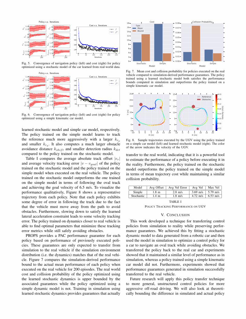
PROPS provides a PAC performance guarantee for eachpolicy based on performance of previously executed poli-cies. These guarantees are only expected to transfer fromsimulation to the real vehicle if the simulation environmentdistribution (i.e. the dynamics) matches that of the real vehi-cle. Figure 7 compares the simulation-derived performancebound to the actual mean performance of each policy whenexecuted on the real vehicle for 200 episodes. The real worldcost and collision probability of the policy optimized usingthe learned stochastic dynamics is upper bounded by theassociated guarantees while the policy optimized using asimple dynamic model is not. Training in simulation usinglearned stochastic dynamics provides guarantees that actually

Stochastic Simple

Model

0

2

4

6

8

10

12

14

16

18Cost

Type

Mean

Bound

Stochastic Simple

Model

0.00

0.01

0.02

0.03

0.04

0.05

0.06

0.07

0.08Collision Probability

Fig. 7. Mean cost and collision probability for policies executed on the realvehicle compared to simulation-derived performance guarantees. The policytrained using a learned stochastic model both satisfies the performancebounds computed in simulation and outperforms the policy trained on asimple kinematic car model.

-10 -5 0 5 10 15 20

X (m)

-5

0

5

10

15

20

25

Y (

m)

-10 -5 0 5 10 15 20

X (m)

-5

0

5

10

15

20

25

Reference

Obstacles

3.2

3.6

4.0

4.4

4.8

5.2

5.6

6.0

Velo

cit

y (

m/s

)

Fig. 8. Sample trajectories executed by the UGV using the policy trainedon a simple car model (left) and learned stochastic model (right). The colorof the arrow indicates the velocity of the UGV.

transfer to the real world, indicating that it is a powerful toolto estimate the performance of a policy before executing it inthe reality. Furthermore, the policy trained on the stochasticmodel outperforms the policy trained on the simple modelin terms of mean trajectory cost while maintaining a similarcollision probability.

Model Avg Offset Avg Vel Error Avg Vel Max VelSimple 1.8 m 2.8 m/s 3.69 m/s 5.79 m/s

Stochastic 1.4 m 1.8 m/s 4.72 m/s 6.53 m/s

TABLE IPOLICY TRACKING PERFORMANCE ON UGV

V. CONCLUSION

This work developed a technique for transferring controlpolicies from simulation to reality while preserving perfor-mance guarantees. We achieved this by fitting a stochasticdynamic model to data generated from a robotic car and thenused the model in simulation to optimize a control policy fora car to navigate an oval track while avoiding obstacles. Wetransferred the policy back to the real car and experimentsshowed that it maintained a similar level of performance as insimulation, whereas a policy trained using a simple kinematiccar model did not. Furthermore, experiments showed thatperformance guarantees generated in simulation successfullytransferred to the real vehicle.

Future research will apply this policy transfer techniqueto more general, unstructured control policies for moreaggressive off-road driving. We will also look at theoreti-cally bounding the difference in simulated and actual policy

performance based on the discrepancy between the learnedmodel and the dynamics training data.

REFERENCES

[1] J. Tobin, R. Fong, A. Ray, J. Schneider, W. Zaremba, and P. Abbeel,“Domain randomization for transferring deep neural networks fromsimulation to the real world,” in IEEE/RSJ International Conferenceon Intelligent Robots and Systems (IROS), pp. 23–30, IEEE, 2017.

[2] OpenAI, “Learning dexterous in-hand manipulation,” 2018.[3] J. Tan, T. Zhang, E. Coumans, A. Iscen, Y. Bai, D. Hafner, S. Bo-

hez, and V. Vanhoucke, “Sim-to-real: Learning agile locomotion forquadruped robots,” arXiv preprint arXiv:1804.10332, 2018.

[4] X. B. Peng, M. Andrychowicz, W. Zaremba, and P. Abbeel, “Sim-to-real transfer of robotic control with dynamics randomization,” arXivpreprint arXiv:1710.06537, 2017.

[5] F. Sadeghi, A. Toshev, E. Jang, and S. Levine, “Sim2real viewpointinvariant visual servoing by recurrent control,” in Proceedings ofthe IEEE Conference on Computer Vision and Pattern Recognition,pp. 4691–4699, 2018.

[6] M. Sheckells, G. Garimella, and M. Kobilarov, “Robust policy searchwith applications to safe vehicle navigation,” in IEEE InternationalConference on Robotics and Automation (ICRA), pp. 2343–2349,IEEE, 2017.

[7] K. S. Narendra and K. Parthasarathy, “Identification and control ofdynamical systems using neural networks,” IEEE Transactions onneural networks, vol. 1, no. 1, pp. 4–27, 1990.

[8] S. Chen, S. Billings, and P. Grant, “Non-linear system identificationusing neural networks,” International journal of control, vol. 51, no. 6,pp. 1191–1214, 1990.

[9] A. Draeger, S. Engell, and H. Ranke, “Model predictive control usingneural networks,” IEEE Control systems, vol. 15, no. 5, pp. 61–66,1995.

[10] S. E. Vt and Y. C. Shin, “Radial basis function neural networkfor approximation and estimation of nonlinear stochastic dynamicsystems,” IEEE Transactions on Neural Networks, vol. 5, no. 4,pp. 594–603, 1994.

[11] C. K. Williams and C. E. Rasmussen, “Gaussian processes for regres-sion,” in Advances in neural information processing systems, pp. 514–520, 1996.

[12] C. M. Bishop, “Bayesian neural networks,” Journal of the BrazilianComputer Society, vol. 4, no. 1, 1997.

[13] R. M. Neal, “Bayesian training of backpropagation networks by thehybrid monte carlo method,” tech. rep., Citeseer, 1992.

[14] M. Deisenroth and C. E. Rasmussen, “Pilco: A model-based anddata-efficient approach to policy search,” in Proceedings of the 28thInternational Conference on machine learning (ICML-11), pp. 465–472, 2011.

[15] A. G. Kupcsik, M. P. Deisenroth, J. Peters, G. Neumann, et al., “Data-efficient generalization of robot skills with contextual policy search,”in Proceedings of the 27th AAAI Conference on Artificial Intelligence,AAAI 2013, pp. 1401–1407, 2013.

[16] S. Levine and P. Abbeel, “Learning neural network policies withguided policy search under unknown dynamics,” in Advances in NeuralInformation Processing Systems, pp. 1071–1079, 2014.

[17] S. Depeweg, J. M. Hernandez-Lobato, F. Doshi-Velez, and S. Udluft,“Learning and policy search in stochastic dynamical systems withbayesian neural networks,” arXiv preprint arXiv:1605.07127, 2016.

[18] A. Rajeswaran, S. Ghotra, B. Ravindran, and S. Levine, “Epopt:Learning robust neural network policies using model ensembles,”arXiv preprint arXiv:1610.01283, 2016.

[19] J. Peters and S. Schaal, “Reinforcement learning by reward-weightedregression for operational space control,” in Proceedings of the 24thinternational conference on Machine learning, pp. 745–750, ACM,2007.

[20] J. Peters, K. Mulling, and Y. Altun, “Relative entropy policy search.,”in AAAI, pp. 1607–1612, Atlanta, 2010.

[21] A. De Luca, G. Oriolo, and C. Samson, “Feedback control of anonholonomic car-like robot,” in Robot motion planning and control,pp. 171–253, Springer, 1998.

[22] G. Garimella, M. Sheckells, and M. Kobilarov, “A stabilizing gyro-scopic obstacle avoidance controller for underactuated systems,” inIEEE 55th Conference on Decision and Control (CDC), pp. 5010–5016, IEEE, 2016.

[23] M. T. Wolf and J. W. Burdick, “Artificial potential functions forhighway driving with collision avoidance,” in IEEE InternationalConference on Robotics and Automation (ICRA), pp. 3731–3736,IEEE, 2008.

[24] O. Brock and O. Khatib, “High-speed navigation using the globaldynamic window approach,” in IEEE International Conference onRobotics and Automation (ICRA), vol. 1, pp. 341–346, IEEE, 1999.