a frequency domain quantitative technique for robust control system design

A Frequency Domain Quantitative Technique for Robust Control System Design

José Luis Guzmán1, José Carlos Moreno2, Manuel Berenguel3, FranciscoRodríguez4, Julián Sánchez-Hermosilla5

1,2,3,4Departamento de Lenguajes y Computación;5Departamento de Ingeniería Rural, University of Almería

Spain

1. Introduction

Most control techniques require the use of a plant model during the design phase inorder to tune the controller parameters. The mathematical models are an approximation ofreal systems and contain imperfections by several reasons: use of low-order descriptions,unmodelled dynamics, obtaining linear models for a specific operating point (working withpoor performance outside of this working point), etc. Therefore, control techniques that workwithout taking into account these modelling errors, use a fixed-structure model and knownparameters (nominal model ) supposing that the model exactly represents the real process,and the imperfections will be removed by means of feedback. However, there exist othercontrol methods called robust control techniques which use these imperfections implicityduring the design phase. In the robust control field such imperfections are called uncertainties,and instead of working only with one model (nominal model), a family of models is usedforming the nominal model + uncertainties. The uncertainties can be classified in parametricor structured and non-parametric or non-structured. The first ones allow representing theuncertainties into the model coefficients (e.g. the value of a pole placed between maximumand minimum limits). The second ones represent uncertainties as unmodelled dynamics (e.g.differences in the orders of the model and the real system) (Morari and Zafiriou, 1989).The robust control technique which considers more exactly the uncertainties is theQuantitative Feedback Theory (QFT). It is a methodology to design robust controllers basedon frequency domain, and was developed by Prof. Isaac Horowitz (Horowitz, 1982; Horowitzand Sidi, 1972; Horowitz, 1993). This technique allows designing robust controllers whichfulfil some minimum quantitative specifications considering the presence of uncertainty inthe plant model and the existence of perturbations. With this theory, Horowitz showed thatthe final aim of any control design must be to obtain an open-loop transfer function withthe suitable bandwidth (cost of feedback) in order to sensitize the plant and reduce theperturbations. The Nichols plane is used to achieve a desired robust design over the specifiedregion of plant uncertainty where the aim is to design a compensator C(s) and a prefilter F(s)(if it is necessary) (see Figure 1), so that performance and stability specifications are achievedfor the family of plants.

17

www.intechopen.com

This chapter presents for SISO (Single Input Single Output) LTI (Linear Time Invariant)systems, a detailed description of this robust control technique and two real experienceswhere QFT has successfully applied at the University of Almería (Spain). It starts witha QFT description from a theoretical point of view, afterwards section 3. 1 is devoted topresent two well-known software tools for QFT design, and after that two real applicationsin agricultural spraying tasks and solar energy are presented. Finally, the chapter ends withsome conclusions.

2. Synthesis of SISO LTI uncertain feedback control systems using QFT

QFT is a methodology to design robust controllers based on frequency domain (Horowitz,1993; Yaniv, 1999). This technique allows designing robust controllers which fulfil somequantitative specifications. The Nichols plane is the key tool for this technique and is used toachieve a robust design over the specified region of plant uncertainty. The aim is to designa compensator C(s) and a prefilter F(s) (if it is necessary), as shown in Figure 1, so thatperformance and stability specifications are achieved for the family of plants ℘(s) describinga plant P(s). Here, the notation a is used to represent the Laplace transform for a time domainsignal a(t).

Fig. 1. Two degrees of freedom feedback system.

The QFT technique uses the information of the plant uncertainty in a quantitative way,imposing robust tracking, robust stability, and robust attenuation specifications (amongothers). The 2DoF compensator {F, C}, from now onwards the s argument will be omittedwhen necessary for clarity, must be designed in such a way that the plant behaviour variationsdue to the uncertainties are inside of some specific tolerance margins in closed-loop. Here, thefamily ℘(s) is represented by the following equation

℘(s) ={

P(s) = k∏

ni=1(s + zi) ∏

mz=1(s2 + 2ξzω0z + ω2

0z)

sN ∏ar=1(s + pr) ∏

bt=1(s2 + 2ξtω0t + ω2

0t): (1)

k ∈ [kmin, kmax], zi ∈ [zi,min, zi,max], pr ∈ [pr,min, pr,max],

ξz ∈ [ξz,min, ξz,max], ω0z ∈ [ω0z,min, ω0z,max],

ξt ∈ [ξt,min, ξt,max], ω0t ∈ [ω0t,min, ω0t,max],

n + m < a + b + N}

A typical QFT design involves the following steps:

392 Robust Control, Theory and Applications

www.intechopen.com

1. Problem specification. The plant model with uncertainty is identified, and a set ofworking frequencies is selected based on the system bandwidth, Ω ={ω1, ω2, ..., ωk}.The specifications (stability, tracking, input disturbances, output disturbances, noise, andcontrol effort) for each frequency are defined, and the nominal plant P0 is selected.

2. Templates. The quantitative information of the uncertainties is represented by a set ofpoints on the Nichols plane. This set of points is called template and it defines a graphicalrepresentation of the uncertainty at each design frequency ω. An example is shown inFigure 2, where templates of a second-order system given by P(s) = k/s(s + a), withk ∈ [1, 10] and a ∈ [1, 10] are displayed for the following set of frequencies Ω ={0.5, 1, 2, 4, 8, 15, 30, 60, 90, 120, 180} rad/s.

3. Bounds. The specifications settled at the first step are translated, for each frequency ω inΩ set, into prohibited zones on the Nichols plane for the loop transfer function L0(jω) =C(jω)P0(jω). These zones are defined by limits that are known as bounds. There exist somany bounds for each frequency as specifications are considered. So, all these bounds foreach frequency are grouped showing an unique prohibited boundary. Figure 3 shows anexample for stability and tracking specifications.

Fig. 2. QFT Template example.

4. Loop shaping. This phase consists in designing the C controller in such a way that thenominal loop transfer function L0(jω) = C(jω)P0(jω) fulfils the bounds calculated in theprevious phase. Figure 3 shows the design of L0 where the bounds are fulfilled at eachdesign frequency.

5. Prefilter. The prefilter F is designed so that the closed-loop transfer function from referenceto output follows the robust tracking specifications, that is, the closed-loop systemvariations must be inside of a desired tolerance range, as Figure 4 shows.

393A Frequency Domain Quantitative Technique for Robust Control System Design

www.intechopen.com

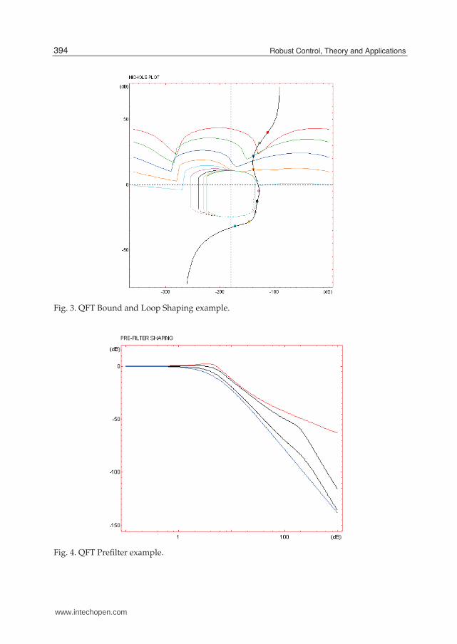
Fig. 3. QFT Bound and Loop Shaping example.

Fig. 4. QFT Prefilter example.


www.intechopen.com

6. Validation. This step is devoted to verify that the closed-loop control system fulfils, forthe whole family of plants, and for all frequencies in the bandwith of the system, all thespecifications given in the first step. Otherwise, new frequencies are added to the set Ω, sothat the design is repeated until such specifications are reached.

The closed-loop specifications for system in Figure 1 are typically defined in time domainand/or in the frequency domain. The time domain specifications define the desired outputsfor determined inputs, and the frequency domain specifications define in terms of frequencythe desired characteristics for the system output for those inputs.In the following, these types of specifications are described and the specifications translationproblem from time domain to frequency domain is considered.

2.1 Time domain specifications

Typically, the closed-loop specifications for system in Figure 1 are defined in terms of thesystem inputs and outputs. Both of them must be delimited, so that the system operates in apredetermined region. For example:

1. In a regulation problem, the aim is to achieve a plant output close to zero (or nearby adetermined operation point). For this case, the time domain specifications could defineallowed operation regions as shown in Figures 5a and 5b, supposing that the aim is toachieve a plant output close to zero.

2. In a reference tracking problem, the plant output must follow the reference input withdetermined time domain characteristics. In Figure 5c a typical specified region is shown,in which the system output must stay. The unit step response is a very commoncharacterization, due to it combines a fast signal (an infinite change in velocity at t = 0+)with a slow signal (it remains in a constant value after transitory).

The classical specifications such as rise time, settling time and maximum overshoot, are specialcases of examples in Figure 5. All these cases can be also defined in frequency domain.

2.2 Frequency domain specifications

The closed-loop specifications for system in Figure 1 are typically defined in terms ofinequalities on the closed-loop transfer functions for the system, as shown in Equations (2)-(7).

1. Disturbance rejection at the plant output:∣

∣

∣

∣

c

do

∣

∣

∣

∣

=

∣

∣

∣

∣

11 + P(jω)C(jω)

∣

∣

∣

∣

≤ δpo(ω) ∀ω > 0, ∀P ∈ ℘ (2)

2. Disturbance rejection at the plant input:∣

∣

∣

∣

c

di

∣

∣

∣

∣

=

∣

∣

∣

∣

P(jω)

1 + P(jω)C(jω)

∣

∣

∣

∣

≤ δpi(ω) ∀ω > 0, ∀P ∈ ℘ (3)

3. Stability:∣

∣

∣

∣

c

rF

∣

∣

∣

∣

=

∣

∣

∣

∣

P(jω)C(jω)

1 + P(jω)C(jω)

∣

∣

∣

∣

≤ λ ∀ω > 0, ∀P ∈ ℘ (4)

4. References Tracking:

Bl(ω) ≤∣

∣

∣

∣

c

r

∣

∣

∣

∣

=

∣

∣

∣

∣

F(jω)P(jω)C(jω)

1 + P(jω)C(jω)

∣

∣

∣

∣

≤ Bu(ω) ∀ω > 0, ∀P ∈ ℘ (5)


www.intechopen.com

0 0.5 1 1.5 2 2.5 3 3.5 4 4.5 5−1

−0.8

−0.6

−0.4

−0.2

0

0.2

0.4

0.6

0.8

1

time (s)

c Allowed operation region

(a) Regulation problem

0 0.5 1 1.5 2 2.5 3 3.5 4 4.5 5−1

−0.8

−0.6

−0.4

−0.2

0

0.2

0.4

0.6

0.8

1

time (s)

c Allowed operation region

(b) Regulation problem for other initial conditions

0 0.5 1 1.5 2 2.5 3 3.5 4 4.5 50

0.2

0.4

0.6

0.8

1

time (s)

c

Allowed operation region

(c) Tracking problem

Fig. 5. Specifications examples in time domain.


www.intechopen.com

5. Noise rejection:∣

∣

∣

∣

c

n

∣

∣

∣

∣

=

∣

∣

∣

∣

P(jω)C(jω)

1 + P(jω)C(jω)

∣

∣

∣

∣

≤ δn(ω) ∀ω > 0, ∀P ∈ ℘ (6)

6. Control effort:∣

∣

∣

∣

u

n

∣

∣

∣

∣

=

∣

∣

∣

∣

C(jω)

1 + P(jω)C(jω)

∣

∣

∣

∣

≤ δce(ω) ∀ω > 0, ∀P ∈ ℘ (7)

For specifications in Eq. (2), (3) and (5), arbitrarily small specifications can be achieveddesigning C so that |C(jω)| → ∞ (due to the appearance of the M-circle in the Nichols plot).So, with an arbitrarily small deviation from the steady state, due to the disturbance, and witha sensibility close to zero, the control system is more independent of the plant uncertainty.Obviously, in order to achieve an increase in |C(jω)| is necessary to increase the crossoverfrequency1 for the system. So, to achieve arbitrarily small specifications implies to increasethe bandwidth2 of the system. Note that the control effort specification is defined, in thiscontext, from the sensor noise n to the control signal u. In order to define this specificationfrom the reference, only the closed-loop transfer function from the n signal to u signal mustbe multiplied by F precompensator. However, in QFT, it is not defined in this form because ofF must be used with other purposes.On the other hand, to increase the value of |C(jω)| implies a problem in the case of thecontrol effort specification and in the case of the sensor noise rejection, since, as was previouslyindicated, the bandwidth of the system is increased (so the sensor noise will affect the systemperformance a lot). A compromise must be achieved among the different specifications.The stability specification is related to the relative stability margins: phase and gain margins.Hence, supposing that λ is the stability specification in Eq. (4), the phase margin is equal to2 · arcsin(0.5λ) degrees, and the gain margin is equal to 20log10(1 + 1/λ) dB.The output disturbance rejection specification limits the distance from the open-loop transferfunction L(jω) to the point (−1, 0) in Nyquist plane, and it sets an upper limit on theamplification of the disturbances at the plan output. So, this type of specification is alsoadequated for relative stability.

2.3 Translation of quantitative specifications from time to frequency domain

As was previously indicated, QFT is a frequency domain design technique, so, when thespecifications are given in the time domain (typically in terms of the unit step response), itis necessary to translate them to frequency domain. One way to do it is to assume a model forthe transfer function Tcr, closed-loop transfer function from reference r to the output c, and tofind values for its parameters so that the defined time domain limits over the system outputare satisfied.

2.3.1 A first-order model

Lets consider the simplest case, a first-order model given by Tcr(s) = K/(s + a), so that whenr(t) is an unit step the system output is given by c(t) = (K/a)(1 − e−at). Then, in order toreach c(t) = r(t) for a time t large enough, K should be K = a.

1 The crossover frequency for a system is defined as the frequency in rad/s such that the magnitude ofthe open-loop transfer function L(jω) = P(jω)C(jω) is equal to zero decibels (dB).

2 The bandwith of a system is defined as the value of the frequency ωb in rad/s such that|Tcr(jωb)/Tcr(0)|dB= -3 dB, where Tcr is the closed-loop transfer function from the reference r to theoutput c.


www.intechopen.com

For a first-order model τc = 1/a = 1/ωb is the time constant (represents the time it takes thesystem step response to reach 63.2% of its final value). In general, the greater the bandwith is,the faster the system output will be.One important difficulty for a first-order model considered is that the first derivative for theoutput (in time infinitesimaly after zero, t = 0+) is c = K, when it would be desirable to be 0.So, problems appear at the neighborhood of time t = 0. In Figure 6 typical specified time limits(from Eq. (5) Bl and Bu are the magnitudes of the frequency response for these time domainlimits) and the system output are shown when a first-order model is used. As observed,problems appear at the neighborhood of time t = 0. On the other hand the first-order modeldoes not allow any overshoot, so from the specified time limits the first order model wouldbe very conservative. Hence, a more complex model must be used for the closed-loop transferfunction Tcr.

0 1 2 3 4 5 6 7 8 9 100

0.2

0.4

0.6

0.8

1

1.2

1.4

1.6

time (s)

Limits

c=2

Fig. 6. Inadequate first-order model.

2.3.2 A second-order model

In this case, two free parameters are available (assuming unit static gain): the damping factorξ and the natural frequency ωn (rad/s). The model is given by

T(s) =ω2

n

s2 + 2ξωns + ω2n

(8)

The unit step response, depending on the value of ξ, is given by


www.intechopen.com

c(t) =

⎧

⎪

⎪

⎨

⎪

⎪

⎩

1 − e−ξωnt(cos(ωn

√

1 − ξ2t) + ξωn

ωn

√1−ξ2

sin(ωn

√

1 − ξ2t)) if ξ < 1

1 − e−ξωnt(cosh(ωn

√

ξ2 − 1t) + ξωn

ωn

√ξ2−1

sinh(ωn

√

1 − ξ2t)) if ξ > 1

1 − e−ξωnt(1 + ωnt) if ξ = 1

In practice, the step response for a system usually has more terms, but normally it containsa dominant second-order component with ξ < 1. The second-order model is very popular incontrol system design in spite of its simplicity, because of it is applicable to a large number ofsystems. The most important time domain indexes for a second-order model are: overshoot,settling time, rise time, damping factor and natural frequency. In frequency domain, its mostimportant indexes are: resonance peak (related with the damping factor and the overshoot),resonance frequency (related with the natural frequency), and the bandwidth (related withthe rise time). The resonance peak is defined as max

ω |Tcr(jω)| � Mp. The resonance frequencyωp is defined as the frequency at which |Tcr(jωp)| = Mp. One way to control the overshootis setting an upper limit over Mp. For example, if this limit is fixed on 3 dB, and the practicalTcr(jω) for ω in the frequency range of interest is ruled by a pair of complex conjugated poles,then this constrain assures an overshoot lower than 27%.In (Horowitz, 1993) tables with these relations are proposed, where, based on the experience ofProfessor Horowitz, makes to set a second-order model to be located inside the allowed zonedefined by the possible specifications. As Horowitz suggested in his book, if the magnitude ofthe closed-loop transfer function Tcr is located between frequency domain limits Bu(ω) andBl(ω) in Eq. (5), then the time domain response is located between the corresponding timedomain specifications, or at most it would be satisfied them in a very approximated way.

2.3.3 A third-order model with a zero

A third-order model with a unit static gain is given by

T(s) =μω3

n

(s2 + 2ξωns + ω2n)(s + μωn)

(9)

For values of μ less than 5, a similar behaviour as if the pole is not added to the second-ordermodel is obtained . So, the model in Eq. (8) would must be used.If a zero is added to Eq. (9), it results

T(s) =(1 + s/λξωn)μω3

n

(s2 + 2ξωns + ω2n)(s + μωn)

(10)

The unit responses obtained in this case are shown in Figure 7 for different values of λ.As shown in Figure 7, this model implies an improvement with respect to that in Eq. (8),because of it is possible to reduce the rise time without increasing the overshoot. Obviously, ifωn > 1, then the response is ωn times faster than the case with ωn = 1 (slower for ωn < 1). In(Horowitz, 1993), several tables are proposed relating parameters in Eq. (10) with time domainparameters as overshoot, rise time and settling time.


www.intechopen.com

0 1 2 3 4 5 6 7 8 9 100

0.2

0.4

0.6

0.8

1

1.2

1.4

1.6

ωn·time

λ=1

λ=0.3

λ=0.5

λ=0.7

Fig. 7. Third-order model with a zero for μ = 5 and ξ = 1.

There exist other techniques to translate specifications from time domain to frequencydomain, such as model-based techniques, where based on the structures of the plant andthe controller, a set of allowed responses is defined. Another technique is that presented in(Krishnan and Cruickshanks, 1977), where the time domain specifications are formulated as∫ t

0 |c(τ) − m(τ)|2dτ ≤∫ t

0 v2(τ)dτ, with m(t) and v(t) specified time domain functions, andwhere it is established that the energy of the signal, difference between the system output andthe specification m(t), must be enclosed by the energy of the signal v(t), for each instant t, andwith a translation to the frequency domain given by the inequality |c(jω)− m(jω)| ≤ |v(jω)|.In (Pritchard and Wigdorowitz, 1996) and (Pritchard and Wigdorowitz, 1997), the relationtime-frequency is studied when uncertainty is included in the system, so that it is possibleto know the time domain limits for the system response from frequency response of a setof closed-loop transfer functions from reference to the output. This technique may be usedto solve the time-frequency translation problem. However, the results obtained in translationfrom frequency to time and from time to frequency are very conservative.

2.4 Controller design

Now, the procedure previously introduced is explained more in detail. The aim is to designthe 2DoF controller {F, G} in Figure 1, so that a subset of specifications introduced in section2.2is satisfied, and the stability of the closed-loop system for all plant P in ℘ is assured.The specifications in section 2. 2are translated in circles on Nyquist plane defining allowedzones for the function L(jω) = P(jω)C(jω). The allowed zone is the outside of the circle forspecifications in Eq. (2)-(6), and the inside one for the specification in Eq. (7). Combining theallowed zones for each function L corresponding to each plant P in ℘, a set of restrictions forcontroller C for each frequency ω is obtained. The limits of these zones represented in Nichols


www.intechopen.com

plane are called bounds or boundaries. These constrains in frequency domain can be formulatedover controller C or over function L0 = P0C, for any plant P0 in ℘ (so-called nominal plant).In order to explain the detailed design process, the following example, from (Horowitz, 1993),is used. Lets suppose the plant in Figure 1 given by

℘ ={

P(s) =k

s(s + a)with k ∈ [1, 20] and a ∈ [1, 5]

}

(11)

corresponding to a range of motors and loads, where the equation modeling the motordynamic is Jc + Bc = Ku, with k = K/J and a = B/J in Eq. (11). Lets suppose the trackingspecifications given by

Bl(ω) ≤ |Tcr(jω)|dB =

∣

∣

∣

∣

F(jω)P(jω)C(jω)

1 + P(jω)C(jω)

∣

∣

∣

∣

dB

≤ Bu(ω) ∀P ∈ ℘ ∀ω > 0 (12)

shown in Figure 8. In Figure 9, the difference δ(ω) = Bu(ω) − Bl(ω) is shown for eachfrequency ω. It is easy to see that in order to satisfy the specifications in Eq. (12), the followinginequality must be satisfied

∆|Tcr(jω)|dB = maxP∈℘

∣

∣

∣

∣

P(jω)C(jω)

1 + P(jω)C(jω)

∣

∣

∣

∣

dB

− minP∈℘

∣

∣

∣

∣

P(jω)C(jω)

1 + P(jω)C(jω)

∣

∣

∣

∣

dB

≤

≤ δ(ω) = Bu(ω)− Bl(ω) ∀P ∈ ℘ ∀ω > 0(13)

10−1

100

101

102

−100

−80

−60

−40

−20

0

20

Frequency (rad/s)

|·| −

dB

Original

Bu(ω)

Bl(ω)

Bu(ω) enlarged

Bl(ω) enlarged

Fig. 8. Tracking specifications (variations over a nominal).


www.intechopen.com

10−1

100

101

102

0

10

20

30

40

50

60

Frequency (rad/s)

Dif.

− d

B

Original

Enlarged

Fig. 9. Specifications on the magnitude variations for the tracking problem.

Making L = PC large enough, for each plant P in ℘, and for a frequency ω, it is possibleto achieve an arbitrarily small specification δ(ω). However, this is not possible in practice,since the system bandwidth must be limited in order to minimize the influence of the sensornoise at the plant input. When C has been designed to satisfy the specifications in Eq. (13), thesecond degree of freedom, F, is used to locate those variations inside magnitude limits Bl(ω)and Bu(ω).In order to design the first degree of freedom, C, it is necessary to define a set of constrains onC or on L0 in the frequency domain, what guarantee that if C (respectively L0) satisfies thoserestrictions then the specifications are satisfied too. As commented above, these constrains arecalled bounds or boundaries in QFT, and in order to compute them it is necessary to take intoaccount:

(i) A set of specifications in frequency domain, that in the case of tracking problem, are givenby Eq. (13), and that in other cases (disturbance rejection, control effort, sensor noise,...) aresimilar as shown in section 2.2.

(ii) An object (representation) modeling the plant uncertainty in frequency domain, so-calledtemplate.

The following sections explain more in detail the meaning of the templates and the bounds.

Computation of basic graphical elements to deal with uncertainties: templates

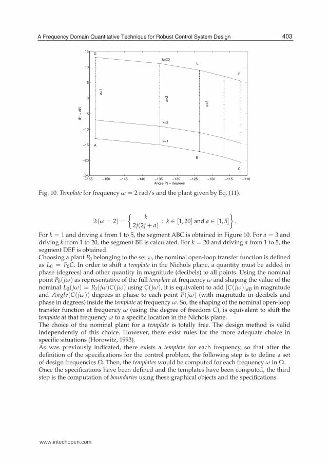
If there is no uncertainty in plant, the set ℘ would contain only one transfer function, P, andfor a frequency, ω, P(jω) would be a point in the Nichols plane. Due to the uncertainty, a setof points, for each frequency, appears in the Nichols plane. One point for each plant P in ℘.These sets are called templates. For example, Figure 10 shows the template for ω = 2 rad/s,corresponding to the set:


www.intechopen.com

−155 −150 −145 −140 −135 −130 −125 −120 −115 −110−25

−20

−15

−10

−5

0

5

10

15

Angle(P) − degrees

|P| −

dB

k=20

k=1

k=2

a=

1

a=

2

a=

3

A

B

C

D

E

F

Fig. 10. Template for frequency ω = 2 rad/s and the plant given by Eq. (11).

ℑ(ω = 2) =

{

k

2j(2j + a): k ∈ [1, 20] and a ∈ [1, 5]

}

.

For k = 1 and driving a from 1 to 5, the segment ABC is obtained in Figure 10. For a = 3 anddriving k from 1 to 20, the segment BE is calculated. For k = 20 and driving a from 1 to 5, thesegment DEF is obtained.Choosing a plant P0 belonging to the set ℘, the nominal open-loop transfer function is definedas L0 = P0C. In order to shift a template in the Nichols plane, a quantity must be added inphase (degrees) and other quantity in magnitude (decibels) to all points. Using the nominalpoint P0(jω) as representative of the full template at frequency ω and shaping the value of thenominal L0(jω) = P0(jω)C(jω) using C(jω), it is equivalent to add |C(jω)|dB in magnitudeand Angle(C(jω)) degrees in phase to each point P(jω) (with magnitude in decibels andphase in degrees) inside the template at frequency ω. So, the shaping of the nominal open-looptransfer function at frequency ω (using the degree of freedom C), is equivalent to shift thetemplate at that frequency ω to a specific location in the Nichols plane.The choice of the nominal plant for a template is totally free. The design method is validindependently of this choice. However, there exist rules for the more adequate choice inspecific situations (Horowitz, 1993).As was previously indicated, there exists a template for each frequency, so that after thedefinition of the specifications for the control problem, the following step is to define a setof design frequencies Ω. Then, the templates would be computed for each frequency ω in Ω.Once the specifications have been defined and the templates have been computed, the thirdstep is the computation of boundaries using these graphical objects and the specifications.


www.intechopen.com

Derivation of boundaries from templates and specifications

Now, zones on Nichols plane are defined for each frequency ω in Ω, so that if the nominal ofthe template shifted by C(jω) is located inside that zone, then the specifications are satisfied.For each specification in section 2. 2and for each frequency ω in Ω, using the template andthe corresponding specification, the boundary must be computed. Details about the differenttypes of bounds and the most important algorithms to compute them can be found in (Morenoet al., 2006). In general, a boundary at frequency ω defines a limit of a zone on Nichols planeso that if the nominal L0(jω) of the shifted template is located inside that zone, then somespecifications are satisfied. So, the most single appearance of a boundary defines a thresholdvalue in magnitude for each phase φ in the Nichols plane, so that if Angle(L0(jω)) = φ, then|L0(jω)|dB must be located above (or below depending on the type of specification used tocompute the boundary) that threshold value.It is important to note that sometimes redefinition of the specifications is necessary. Forexample, for system in Eq. (11), for ω ≥ 10 rad/s the templates have similar dimensions, andthe specifications from Eq. (13) in Figure 9 are identical. Then, the boundaries for ω ≥ 10 rad/swill be almost identical. The function L0(jω) must be above the boundaries for all frequencies,including ω ≥ 10 rad/s, but this is unviable due to it must be satisfied that L0(jω) → 0when ω → ∞. Therefore, it is necessary to open the tracking specifications for high frequency(where furthermore the uncertainty is greater), such as it is shown in Figure 8. On the otherhand, it must be also taken into account that for a large enough frequency ω, the specification

δ(ω) in Eq. (13) must be greater or equal than maxP∈℘ |P(jω)|dB− min

P∈℘ |P(jω)|dB such that, fora small value of L0(jω) for these frequencies, the specifications are also satisfied. The effectof this enlargement for the specifcations is negligible when the modifications are introducedat a frequency large enough. These effects are notable in the response at the neighborhood oft = 0.Considering the tracking bounds as negligible from a specific frequency (in the sense thatthe specification is large enough), it implies that the stability boundaries are the dominantones at these frequencies. As was mentioned above, since the templates are almost identical athigh frequencies and the stability specification λ is independent of the frequency, the stabilitybounds are also identical and only one of them can be used as representative of the rest. InQFT, this boundary is usually called high frequency bound, and it is denoted by Bh.Notice that the use of a discrete set of design frequencies Ω does not imply any problem.The variation of the specifications and the variation of the appearance of the templates from afrequency ω− to a frequency ω+, with ω− < ω < ω+, is smooth. Anyway, the methodologylet us discern the specific cases in which the number of elements of Ω is insufficient, and letus iterate in the design process to incorporate the boundaries for those new frequencies, thenreshaping again the compensator {F, C}.

Design of the nominal open-loop transfer function fulfilling the boundaries

In this stage, the function L0(jω) must be shaped fulfilling all the boundaries for each frequency.Furthermore, It must assure that the transfer function 1 + L(s) has no zeros in the right halfplane for any plant P in ℘. So, initially L0 = P0 (C = 1) and poles and zeros are added to thisfunction (poles and zeros of the controller C) in order to satisfy all of these restrictions on theNichols plane. In this stage, only using the function L0, it is possible to assure the fulfillment ofthe specifications for all of the elements in the set ℘ when L0(jω) is located inside the allowedzones defined by the boundary at frequency ω (computed from the corresponding template atthat frequency, and from the specifications).


www.intechopen.com

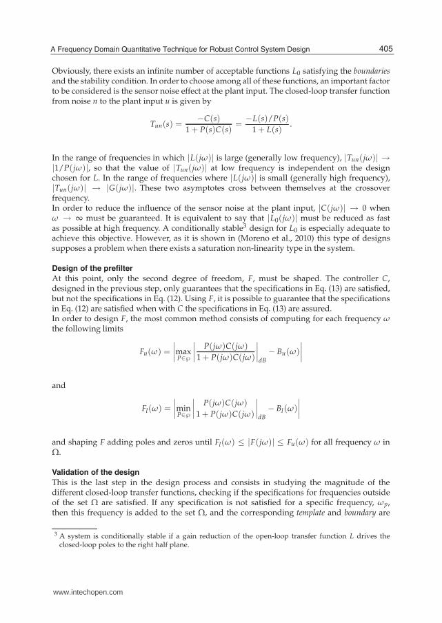
Obviously, there exists an infinite number of acceptable functions L0 satisfying the boundariesand the stability condition. In order to choose among all of these functions, an important factorto be considered is the sensor noise effect at the plant input. The closed-loop transfer functionfrom noise n to the plant input u is given by

Tun(s) =−C(s)

1 + P(s)C(s)=

−L(s)/P(s)

1 + L(s).

In the range of frequencies in which |L(jω)| is large (generally low frequency), |Tun(jω)| →|1/P(jω)|, so that the value of |Tun(jω)| at low frequency is independent on the designchosen for L. In the range of frequencies where |L(jω)| is small (generally high frequency),|Tun(jω)| → |G(jω)|. These two asymptotes cross between themselves at the crossoverfrequency.In order to reduce the influence of the sensor noise at the plant input, |C(jω)| → 0 whenω → ∞ must be guaranteed. It is equivalent to say that |L0(jω)| must be reduced as fastas possible at high frequency. A conditionally stable3 design for L0 is especially adequate toachieve this objective. However, as it is shown in (Moreno et al., 2010) this type of designssupposes a problem when there exists a saturation non-linearity type in the system.

Design of the prefilter

At this point, only the second degree of freedom, F, must be shaped. The controller C,designed in the previous step, only guarantees that the specifications in Eq. (13) are satisfied,but not the specifications in Eq. (12). Using F, it is possible to guarantee that the specificationsin Eq. (12) are satisfied when with C the specifications in Eq. (13) are assured.In order to design F, the most common method consists of computing for each frequency ωthe following limits

Fu(ω) =

∣

∣

∣

∣

maxP∈℘

∣

∣

∣

∣

P(jω)C(jω)

1 + P(jω)C(jω)

∣

∣

∣

∣

dB

− Bu(ω)

∣

∣

∣

∣

and

Fl(ω) =

∣

∣

∣

∣

minP∈℘

∣

∣

∣

∣

P(jω)C(jω)

1 + P(jω)C(jω)

∣

∣

∣

∣

dB

− Bl(ω)

∣

∣

∣

∣

and shaping F adding poles and zeros until Fl(ω) ≤ |F(jω)| ≤ Fu(ω) for all frequency ω inΩ.

Validation of the design

This is the last step in the design process and consists in studying the magnitude of thedifferent closed-loop transfer functions, checking if the specifications for frequencies outsideof the set Ω are satisfied. If any specification is not satisfied for a specific frequency, ωp,then this frequency is added to the set Ω, and the corresponding template and boundary are

3 A system is conditionally stable if a gain reduction of the open-loop transfer function L drives theclosed-loop poles to the right half plane.


www.intechopen.com

computed for that frequency ωp. Then, the function L0 is reshaped, so that the new restrictionis satisfied. Afterwards, the precompensator F is reshaped, and finally the new design isvalidated. So, an iterative procedure is followed until the validation result is satisfactory.

3. Computer-based tools for QFT

As it has been described in the previous section, the QFT framework evolves severalstages, where a continuous re-design process must be followed. Furthermore, there are somesteps requiring the use of algorithms to calculate the corresponding parameters. Therefore,computer-based tools as support for the QFT methodology are highly valuable to help inthe design procedure. This section briefly describes the most well-known tools available inthe literature, The Matlab QFT Toolbox (Borghesani et al., 2003) and SISO-QFTIT (Díaz et al.,2005a),(Díaz et al., 2005b).

3.1 Matlab QFT toolbox

The QFT Frequency Domain Control Design Toolbox is a commercial collection of Matlabfunctions for designing robust feedback systems using QFT, supported by the companyTerasoft, Inc (Borghesani et al., 2003). The QFT Toolbox includes a convenient GUI thatfacilitates classical loop shaping of controllers to meet design requirements in the face ofplant uncertainty and disturbances. The interactive GUI for shaping controllers providesa point-click interface for loop shaping using classical frequency domain concepts. Thetoolbox also includes powerful bound computation routines which help in the conversion ofclosed-loop specifications into boundaries on the open-loop transfer function (Borghesani et al.,2003).The toolbox is used as a combination of Matlab functions and graphical interfaces to performa complete QFT design. The best way to do that is to create a Matlab script including all therequired calls to the corresponding functions. The following lines briefly describe the mainsteps and functions to use, where an example presented in (Borghesani et al., 2003) is followedfor a better understanding (a more detailed description can be found in (Borghesani et al.,2003)).The example to follow is described by:

℘ ={

P(s) =k

(s + a)(s + b): k = [1, 2, 5, 8, 10], a = [1, 3, 5], b = [20, 25, 30]

}

. (14)

Once the process and the associated uncertainties are defined, the different steps, explainedin section 2., to design the robust control scheme using the QFT toolbox are described in thefollowing:

• Template computation. First, the transfer function models representing the processuncertainty must be written. The following code calculates a matrix of 40 plant elementswhich is stored in the variable P and represents the system defined by Eq. (14).

» c = 1; k = 10; b = 20;» for a = linspace(1,5,10),» P(1,1,c) = tf(k,[1,a+b,a*b]); c = c + 1;» end» k = 1; b = 30;» for a = linspace(1,5,10),


www.intechopen.com

» P(1,1,c) = tf(k,[1,a+b,a*b]); c = c + 1;» end» b = 30; a = 5;» for k = linspace(1,10,10),» P(1,1,c) = tf(k, [1,a+b,a*b]); c = c + 1;» end» b = 20; a = 1;» for k = linspace(1,10,10),» P(1,1,c) = tf(k, [1,a+b,a*b]); c = c + 1;» end

Then, the nominal element is selected:» nompt=21;

and the frequency array is set:» w = [0.1, 5, 10, 100];

Finally, the templates are calculated and visualized using the plottmpl function (see(Borghesani et al., 2003) for a detailed explanation):

» plottmpl(w,P,nompt);obtaining the templates shown in Figure 11.

Fig. 11. Matlab QFT Toolbox. Templates for example in Eq. (14)

• Specifications. In this step, the system specifications must be defined according to Eq. (2)-(7).Once the specifications are determined, the corresponding bounds on the Nichols plane arecomputed. The following source code shows the use of specifications in Eq. (2)-(4) for thisexample.A stability specification of λ = 1.2 in Eq. (4) corresponding to a gain margin (GM) ≥ 5.3dB and a phase margin (PM) = 49.25 degrees is given:

» Ws1 = 1.2;Then, the stability bounds are computed using the function sisobnds (see (Borghesani et al.,2003) for a detailed explanation) and its value is stored in the variable bdb1:


www.intechopen.com

» bdb1 = sisobnds(1,w,Ws1,P,0,nompt);Lets now consider the specifications for output and input disturbance rejection cases, fromEq. (2)-(3). For the case of the output disturbance specification, the performance weight forthe bandwidth [0,10] is defined as

» Ws2 = tf(0.02*[1,64,748,2400],[1,14.4,169]);and the bounds are computed in the following way

» bdb2 = sisobnds(2,w(1:3),Ws2,P,0,nompt);For the input disturbance case, the specification is defined as constant for

» Ws3 = 0.01;calculating the bounds as

» bdb3 = sisobnds(3,w(1:3),Ws3,P,0,nompt);also for the bandwidth [0,10].Once the specifications are defined and the corresponding bounds are calculated. For eachfrequency they can be combined using the following functions:

» bdb = grpbnds(bdb1,bdb2,bdb3); // Making a global structure» ubdb = sectbnds(bdb); // Combining bounds

The resulting bounds which will be used for the loop-shaping stage are shown in Figure 12.This figure is obtained using the plotbnds function:

» plotbnds(ubdb);

Fig. 12. Matlab QFT Toolbox. Boundaries for example (14)

• Loop-shaping. After obtaining the stability and performance bounds, the next step consists indesigning (loop shaping) the controller. The QFT toolbox includes a graphical interactiveGUI, l pshape, which helps to perform this task in an straightforward way. Before usingthis function, it is necessary to define the frequency array for loop shaping, the nominalplant, and the initial controller transfer function. Therefore, these variables must be setpreviously, where for this example are given by:

» wl = logspace(-2,3,100); // frequency array for loop shaping» C0 = tf(1,1); // Initial Controller


www.intechopen.com

» L0=P(1,1,nompt)*C0; // Nominal open-loop transfer functionHaving defined these variables, the graphical interface is opened using the following line:

» lpshape(wl,ubdb,L0,C0);obtaining the window shown in Figure 13. As shown from this figure, the GUI allows tomodify the control transfer functions adding, modifying, and removing poles and zeros.This task can be done from the options available at the right area of the windows ordragging interactively on the loop L0(s) = P0(s)C(s) represented by the black line onthe Nichols plane.For this example, the final controller is given by (Borghesani et al., 2003)

C(s) =379( s

42 + 1)s2

2472 + s247 + 1

(15)

Fig. 13. Matlab QFT Toolbox. Loop shaping for example in Eq. (14)

• Pre-filter design. When the control design requires tracking of reference signals, althoughthis is not the case for this example, a pre-filter F(s) must be used in addition tothe controller C(s) such as discussed in section 2.. The prefilter can be also designedinteractively using a graphical interface similar to that described for the loop shaping stage.To run this option, the p f shape function must be used (see (Borghesani et al., 2003) for moredetails).

• Validation. The control system validation can be done testing the resulting robust controllerfor all uncertain plants defined by Eq. (14) and checking that the different specificationsare fulfilled for all of them. This task can be performed directly programming in Matlab orusing the chksiso function from the QFT toolbox.

3.2 An interactive tool based in Sysquake: SISO-QFTIT

SISO-QFTIT is a free software interactive tool for robust control design using the QFTmethodology (Díaz et al., 2005a;b). The main advantages of SISO-QFTIT compared to otherexisting tools are its easiness of use and its interactive nature. In the tool described in theprevious section, a combination between code and graphical interfaces must be used, where


www.intechopen.com

some interactive features are also provided for the loop shaping and filter design stages.However, with SISO-QFTIT all the stages are available from an interactive point of view.As commented above, the tool has been implemented in Sysquake, a Matlab-like languagewith fast execution and excellent facilities for interactive graphics (Piguet, 2004). Windows,Mac, and Linux operating systems are supported. Since this tool is completely interactive, oneconsideration that must be kept in mind is that the tool’s main feature -interactivity- cannotbe easily illustrated in a written text. Thus, the reader is cordially invited to experience theinteractive features of the tool.The users mainly should operate with only mouse operations on different elements in thewindow of the application or text insertion in dialog boxes. The actions that they carry out arereflected instantly in all the graphics in the screen. In this way the users take aware visuallyof the effects that produce their actions on the design that they are carrying out. This tool isspecially conceived as much as for beginner users that want to learn the QFT methodology, asfor expert users (Díaz et al., 2005b).The user can work with SISO-QFTIT in two different but not excluding ways (Díaz et al.,2005b):

• Interactive mode. In this work form, the user selects an element in the window and dragsit to take it to a certain value, their actions on this element are reflected simultaneously onall the present figures in the window of the tool.

• Dialogue mode. In this work form, the user should simply go selecting entrances of theSettings menu and correctly fill the blanks of dialog boxes.

Such as commented in the manual of this interactive software tool, its main interactiveadvantages and options are the following (Díaz et al., 2005b):

• Variations that take place in the templates when modifying the uncertainty of the differentelements of the plant or in the value of the template calculation frequency.

• Individual or combined variation on the bounds as a result of the configuration ofspecifications, i.e., by adding zeros and poles to the different specifications.

• The movement of the controller zeros and poles over the complex plane and themodification of its symbolic transfer function when the open loop transfer function ismodified in the Nichols plane.

• The change of shape of the open loop transfer function in the Nichols plane and thevariation of the expression of the controller transfer function when any movement,addition or suppression of its zeros or poles in the complex plane.

• The changes that take place in the time domain representation of the manipulated andcontrolled variables due to the modification of the nominal values of the different elementsof the plant.

• The changes that take place in the time domain representation of the manipulated andcontrolled variables due to the introduction of a step perturbation at the input of the plant.The magnitude and the occurrence instant of the perturbation is configured by the user bymeans of the mouse.

Such as pointed out above, the interactive capabilities of the tool cannot be shown in awritten text. However, some screenshots for the example used with the Matlab QFT toolboxare provided. Figure 14a shows the resulting templates for the process defined by Eq. (14).


www.intechopen.com

Notice that with this tool, the frequencies, the process uncertainties and the nominal plantcan be interactively modified. The stability bounds are shown in Figure 14b. The radiobuttonsavailable at the top-right side of the tool allow to choose the desired specification. Once thespecification is selected, the rest of the screen is changed to include the specification valuesin an interactive way. Figure 15a displays the loop shaping stage with the combination ofthe different bounds (same result than in Figure 13). The figure also shows the resulting loopshaping for controller (15). Then, the validation screen is shown in Figure 15b, where it ispossible to check interactively if the robust control design satisfies the specifications for alluncertain cases. Although for this example it is not necessary to design the pre-filter for thetracking specifications, this tool also provides a screen where it is possible to perform this task(see an example in Figure 16).

(a) QFT Templates (b) Stability bounds

Fig. 14. SISO-QFTIT. Templates and bounds for the example described in Eq. (14)

(a) Loop shaping (b) Validation

Fig. 15. SISO-QFTIT. Loop shaping and validation for the example described in Eq. (14)

4. Practical applications

This section presents two industrial projects where the QFT technique has been successfullyused. The first one is focused on the pressure control of a mobile robot which was design


www.intechopen.com

Fig. 16. SISO-QFTIT. Prefilter stage

for spraying tasks in greenhouses (Guzmán et al., 2008). The second one deals with thetemperature control of a solar collector field (Cirre et al., 2010).

4.1 In agricultural and robotics context: Fitorobot

During the last six years, the Automatic Control, Robotics and Electronics research groupand the Agricultural Engineering Department, both from the University of Almería (Spain),have been working in a project aimed at designing, implementation, and testing a multi-useautonomous vehicle with safe, efficient, and economic operation which moves through thecrop lines of a greenhouse and which performs tasks that are tedious and/or hazardous forpeople. This robot has been called Fitorobot. The first version of this vehicle has been equippedfor spraying activities, but other configurations have also been designed, such as: a liftingplatform to reach high zones to perform tasks (staking, cleaning leaves, harvesting, manualpollination, etc.), and a forklift to transport and raise heavy materials (Sánchez-Gimeno et al.,2006). This mobile robot was designed and built following the paradigm of Mechatronics suchas described in (Sánchez-Hermosilla. et al., 2010).The first objective of the project consisted of developing a prototype to enable the sprayingof a certain volume of chemical products per hectare while controlling the different variablesthat affect the spraying system (pressure, flow, and travel speed). The pressure is selected andthe control signal keeps the spraying conditions constant (mainly droplet size). The referencevalue of the pressure is calculated based on the mobile robot speed and the volume of pesticideto apply, where the pressure working range is between 5 and 15 bar.There are some circumstances where it is impossible to maintain a constant velocity dueto the irregularities of the soil, different slopes of the ground, and the turning movementsbetween the crop lines. Thus, for work at a variable velocity (Guzmán et al., 2008), it isnecessary to spray using a variable-pressure system based on the vehicle velocity, which isthe proposal adopted and implemented in this work. This system presents some advantages,such as the higher quality of the process, because the product sprayed over each plant isoptimal. Furthermore, this system saves chemical products because an optimal quantity issprayed, reducing the environmental impact and pollution as the volume sprayed to the air isminimized.The robot prototype (Figure 17) consists of an autonomous mobile platform with a rubbertracked system and differential guidance mechanism (to achieve a more homogeneous


www.intechopen.com

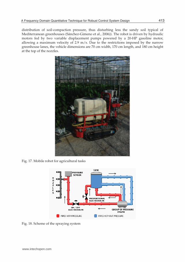
distribution of soil-compaction pressure, thus disturbing less the sandy soil typical ofMediterranean greenhouses (Sánchez-Gimeno et al., 2006)). The robot is driven by hydraulicmotors fed by two variable displacement pumps powered by a 20-HP gasoline motor,allowing a maximum velocity of 2.9 m/s. Due to the restrictions imposed by the narrowgreenhouse lanes, the vehicle dimensions are 70 cm width, 170 cm length, and 180 cm heightat the top of the nozzles.

Fig. 17. Mobile robot for agricultural tasks

Fig. 18. Scheme of the spraying system


www.intechopen.com

The spraying system carried out by the mobile robot is composed with a 300 l tank used tostore the chemical products, a vertical boom sprayer with 10 nozzles, an on/off electrovalveto activate the spraying, a proportional electrovalve to regulate the output pressure, adouble-membrane pump with pressure accumulator providing a maximum flow of 30 l/minand a maximum pressure of 30 bar, and a pressure sensor to close the control loop as shownin Figure 18.In this case, the control problem was focused on regulating the output pressure of thespraying system mounted on the mobile robot despite changes in the vehicle velocity andthe nonlinearities of the process.For an adequate control system design, it was necessary to model the plant by obtaining itsassociated parameters. Several open-loop step-based tests were performed varying the valveaperture around a particular operating point. The results showed that the system dynamicscan be approximated by a first-order system with delay. Thus, it can be modelled using thefollowing transfer function

P(s) =k

τs + 1e−trs (16)

where k is the static gain, tr is the delay time, and τ is the time constant.Then, several experiments in open loop were performed to design the dynamic model ofthe spraying system using different amplitude opening steps (5% and 10%) over the sameoperating points (see Figure 19a). The analysis of the results showed that the output-pressurebehavior changes when different valve-amplitude steps are produced around the sameworking point, and also when the same valve opening steps are produced at several operatingpoints, confirming the uncertainty and nonlinear characteristics of the system.

(a) Time domain

−100

−80

−60

−40

−20

0

Ma

gn

itu

de

(d

B)

10−2

10−1

100

101

102

103

−180

−90

0

90

180

Ph

ase

(d

eg

)

(b) Frequency domain

Fig. 19. System uncertainties from the time and frequency domains

After analyzing the results (see Figure 19a), the system was modelled as a first-orderdynamical system with uncertain parameters, where the reaction curve method has beenused at the different operating points. Therefore, the resulting uncertain model is given bythe following transfer function (see Figure 19b):

℘ ={

P(s) =k

τs + 1: k ∈ [−0.572,−0.150], τ ∈ [0.4, 1]

}

(17)


www.intechopen.com

where the gain, k, is given in bar/% aperture and the constant time, τ , in seconds.Once the system was characterized, the robust control design using QFT was performedconsidering specifications on stability and tracking.First, the specifications for each frequency were defined, and the nominal plant P0 wasselected. The set of frequencies and the nominal plant were set to Ω = {0.1, 1, 2, 10} rad/sand P0 = −0.3

0.7s+1 , respectively. The stability specification was set to λ = 1.2 correspondingto a GM ≥ 5.3 dB and a PM = 49.25, and for the tracking specifications the maximum andminimum values for the magnitude have been described by the following transfer functions(frequency response for tracking specifications are shown in Figure 19b in dashed lines)

Bl(s) =10

s + 10, Bu(s) =

12.25s2 + 8.75s + 12.25

(18)

Figure 20a shows the different templates of the plant for the set of frequencies determinedabove.

(a) QFT Templates (b) Loopshaping stage

Fig. 20. Templates and feedback controller design by QFT

The specifications are translated to the boundaries on the Nichols plane for the loop-transferfunction L(jω) = C(jω)P(jω). Figure 20b shows the different bounds for stability and trackingspecifications set previously.Then, the loop shaping stage was performed in such a way that the nominal loop-transferfunction L0(jω) = C(jω)P0(jω) was adjusted to make the templates fulfil the boundscalculated in the previous phase. Figure 20b shows the design of L0 where the bounds arefulfilled at each design frequency. This figure shows the optimal controller using QFT tolie on the boundaries at each frequency design. However, a simpler controller fulfilling thespecifications was preferred for practical reasons. The resulting controller was the following:

C(s) =27.25(s + 1)

s(19)

To conclude the design process, the prefilter F is determined so that the closed-loop transferfunction matches the robust tracking specifications, that is, the closed-loop system variationsmust be inside of a desired tolerance range:

F(s) =1

0.1786s + 1(20)


www.intechopen.com

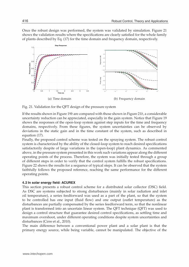
Once the robust design was performed, the system was validated by simulation. Figure 21shows the validation results where the specifications are clearly satisfied for the whole familyof plants described by Eq. (17) for the time domain and frequency domain, respectively.

0 0.5 1 1.5 2 2.5 3 3.50

0.2

0.4

0.6

0.8

1

1.2

Time (s)

Pre

ssu

re (

bar)

Step Response

(a) Time domain

−100

−80

−60

−40

−20

0

Magnitude (

dB

)

10−2

10−1

100

101

102

103

−180

−135

−90

−45

0

Phase (

deg)

(b) Frequency domain

Fig. 21. Validation for the QFT design of the pressure system

If the results shown in Figure 19b are compared with those shown in Figure 21b, a considerableuncertainty reduction can be appreciated, especially in the gain system. Notice that Figure 19shows the responses of the open-loop system against step inputs for the time and frequencydomains, respectively. From these figures, the system uncertainties can be observed bydeviations in the static gain and in the time constant of the system, such as described inequation (17).Finally, the proposed control scheme was tested on the spraying system. The robust controlsystem is characterized by the ability of the closed-loop system to reach desired specificationssatisfactorily despite of large variations in the (open-loop) plant dynamics. As commentedabove, in the pressure system presented in this work such variations appear along the differentoperating points of the process. Therefore, the system was initially tested through a groupof different steps in order to verify that the control system fulfills the robust specifications.Figure 22 shows the results for a sequence of typical steps. It can be observed that the systemfaithfully follows the proposed reference, reaching the same performance for the differentoperating points.

4.2 In solar energy field: ACUREX

This section presents a robust control scheme for a distributed solar collector (DSC) field.As DSC are systems subjected to strong disturbances (mainly in solar radiation and inletoil temperature), a series feedforward was used as a part of the plant, so that the systemto be controlled has one input (fluid flow) and one output (outlet temperature) as thedisturbances are partially compensated by the series feedforward term, so that the nonlinearplant is transformed into an uncertain linear system. The QFT technique (QFT) was used todesign a control structure that guarantee desired control specifications, as settling time andmaximum overshoot, under different operating conditions despite system uncertainties anddisturbances (Cirre et al., 2010).The main difference between a conventional power plant and a solar plant is that theprimary energy source, while being variable, cannot be manipulated. The objective of the


www.intechopen.com

50 100 150 200 250

6

8

10

12

14

Time (s)

Pre

su

re (

ba

r)

Set−point

Pressure

50 100 150 200 250

40

45

50

55

60

65

Time (s)

Co

ntr

ol

sig

na

l (%

)

Fig. 22. Experimental tests for the spraying system

control system in a distributed solar collector field (DCS) is to maintain the outlet oiltemperature of the loop at a desired level in spite of disturbances such as changes in thesolar irradiance level (caused by clouds), mirror reflectivity, or inlet oil temperature. Themeans available for achieving this is via the adjustment of the fluid flow and the daily solarpower cycle characteristics are such that the oil flow has to change substantially duringoperation. This leads to significant variations in the dynamic characteristics of the field, whichcause difficulties in obtaining adequate performance over the operating range with a fixedparameter controller (Camacho et al., 1997; 2007a;b). For that reason, this section summarizesa work developed by the authors where a robust PID controller is designed to control theoutlet oil temperature of a DSC loop using the QFT technique.In this work, the ACUREX thermosolar plant was used, which is located at the PlataformaSolar de Almería (PSA), a research centre of the Spanish Centro de Investigaciones EnergéticasMedioambientales y Tecnológicas (CIEMAT), in Almería, Spain. The plant is schematicallycomposed of a distributed collector field, a recirculation pump, a storage tank and athree-way valve, as shown in Figures 23 and 24. The distributed collector field consists of 480east-west-aligned single-axis-tracking parabolic trough collectors, with a total mirror aperturearea of 2672 m2, arranged in 20 rows forming 10 parallel loops (see Figure 23). The parabolicmirrors in each collector concentrate the solar irradiation on an absorber tube through whichSantotherm 55 heat transfer oil is flowing. For the collector to concentrate sunlight on its focus,the direct solar radiation must be perpendicular to the mirror plane. Therefore, a sun-tracking


www.intechopen.com

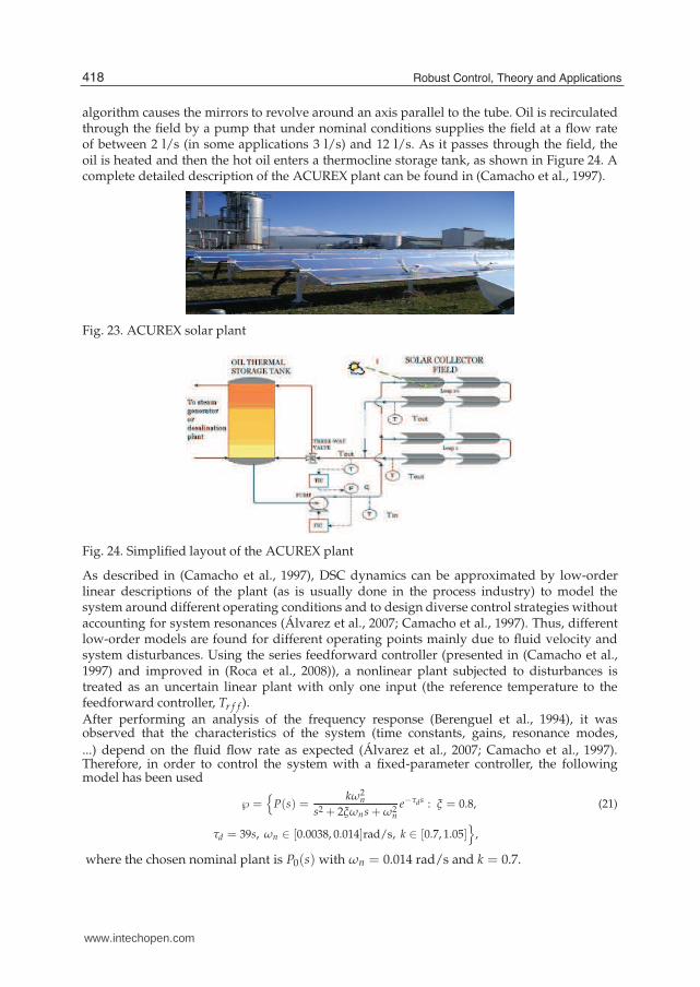
algorithm causes the mirrors to revolve around an axis parallel to the tube. Oil is recirculatedthrough the field by a pump that under nominal conditions supplies the field at a flow rateof between 2 l/s (in some applications 3 l/s) and 12 l/s. As it passes through the field, theoil is heated and then the hot oil enters a thermocline storage tank, as shown in Figure 24. Acomplete detailed description of the ACUREX plant can be found in (Camacho et al., 1997).

Fig. 23. ACUREX solar plant

Fig. 24. Simplified layout of the ACUREX plant

As described in (Camacho et al., 1997), DSC dynamics can be approximated by low-orderlinear descriptions of the plant (as is usually done in the process industry) to model thesystem around different operating conditions and to design diverse control strategies withoutaccounting for system resonances (Álvarez et al., 2007; Camacho et al., 1997). Thus, differentlow-order models are found for different operating points mainly due to fluid velocity andsystem disturbances. Using the series feedforward controller (presented in (Camacho et al.,1997) and improved in (Roca et al., 2008)), a nonlinear plant subjected to disturbances istreated as an uncertain linear plant with only one input (the reference temperature to thefeedforward controller, Tr f f ).After performing an analysis of the frequency response (Berenguel et al., 1994), it wasobserved that the characteristics of the system (time constants, gains, resonance modes,...) depend on the fluid flow rate as expected (Álvarez et al., 2007; Camacho et al., 1997).Therefore, in order to control the system with a fixed-parameter controller, the followingmodel has been used

℘ ={

P(s) =kω2

n

s2 + 2ξωns + ω2n

e−τds : ξ = 0.8, (21)

τd = 39s, ωn ∈ [0.0038, 0.014]rad/s, k ∈ [0.7, 1.05]}

,

where the chosen nominal plant is P0(s) with ωn = 0.014 rad/s and k = 0.7.


www.intechopen.com

Thus, once the uncertain model has been obtained, the specifications were determined on timedomain and translated into the frequency domain for the QFT design. In this case, the trackingand stability specifications were established (Horowitz, 1993). For tracking specificationsonly is necessary to impose the minimum and maximum values for the magnitude of theclosed-loop transfer function from the reference input to the output in all frequencies. Withrespect to the stability specification, the desired gain (GM) and phase (PM) margins are set.The tracking specifications were required to fulfill a settling time between 5 and 35 minutesand an overshoot less than 30% after 10-20oC setpoint changes for all operating conditions(realistic specifications, see (Camacho et al., 2007a;b)).For stability specification, λ = 3.77 in Eq. (4) is selected in order to guarantee at least a phasemargin of 35 degrees for all operating conditions.To design the compensator C(s), the tracking specifications in Eq. (13), shown in Table 1 foreach frequency in the set of design frequencies Ω, are used

Table 1. Tracking specifications for the C compensator design

ω (rad/s) 0.0006 0.001 0.003 0.01δ(ω) 0.55 1.50 9.01 19.25

The resulting compensator C(s), synthesized in order to achieve the stability specificationsand the tracking specifications previously indicated, is the following PID-type controller

C(s) = 0.75(

1 +1

180s+ 40s

)

(22)

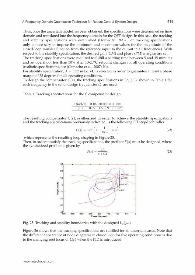
which represents the resulting loop shaping in Figure 25.Then, in order to satisfy the tracking specifications, the prefilter F(s) must be designed, wherethe synthesized prefilter is given by

F(s) =0.1

s + 0.1(23)

Fig. 25. Tracking and stability boundaries with the designed L0(jω)

Figure 26 shows that the tracking specifications are fulfilled for all uncertain cases. Note thatthe different appearance of Bode diagrams in closed loop for five operating conditions is dueto the changing root locus of L(s) when the PID is introduced.


www.intechopen.com

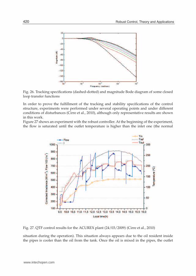
Fig. 26. Tracking specifications (dashed-dotted) and magnitude Bode diagram of some closedloop transfer functions

In order to prove the fulfillment of the tracking and stability specifications of the controlstructure, experiments were performed under several operating points and under differentconditions of disturbances (Cirre et al., 2010), although only representative results are shownin this work.Figure 27 shows an experiment with the robust controller. At the beginning of the experiment,the flow is saturated until the outlet temperature is higher than the inlet one (the normal

Fig. 27. QTF control results for the ACUREX plant (24/03/2009) (Cirre et al., 2010)

situation during the operation). This situation always appears due to the oil resident insidethe pipes is cooler than the oil from the tank. Once the oil is mixed in the pipes, the outlet


www.intechopen.com

temperature reaches a higher temperature than the inlet one. During the start up, steps in thereference temperature are made until reaching the nominal operating point. The overshootat the end of this phase is 18 oC approximately, and thus the specifications are fulfilled.Analyzing the time responses, a settling time between 11 and 15 minutes is observed at thedifferent operating points. Therefore, both time specifications, overshoot and settling time areproperly fulfilled. Disturbances in the inlet temperature (from the beginning until t = 12.0 h),due to the temperature variation of the stratified oil inside the tank, are observed during thisexperiment and correctly rejected by the feedforward action (Cirre et al., 2010).

5. Conclusions

This chapter has introduced the Quantitative Feedback Theory as a robust controltechnique based on the frequency domain. QFT is a powerful tool which allows to designrobust controllers considering the plant uncertainty, disturbances, noise and the desiredspecifications. It is very versatile tool and has been used in multiple control problemsincluding linear (Horowitz, 1963), non-linear (Moreno et al., 2010), (Moreno et al., 2003),(Moreno, 2003), MIMO (Horowitz, 1979) and non-minimum phase (Horowitz and Sidi, 1978).After describing the theoretical aspects, the most well-known software tools to work with QFThave been described using simple examples. Then, results from two experimental applicationswere presented, where QFT were successfully used to compensate for the uncertainties in theprocesses.

6.References

J.D. Álvarez, L. Yebra, and M. Berenguel. Repetitive control of tubular heat exchangers. Journalof Process Control, 17:689–701, 2007.

M. Berenguel, E.F. Camacho, and F.R. Rubio. Simulation software package for the acurex field.Technical report, Dep. Ingeniería de Sistemas y Automática, University of Seville(Spain), 1994. www.esi2.us.es/ rubio/libro2.html.

C. Borghesani, Y. Chait, and O. Yaniv. The QFT Frequency Domain Control Design Toolbox.Terasoft, Inc., http://www.terasoft.com/qft/QFTManual.pdf, 2003.

E.F. Camacho, M. Berenguel, and F.R. Rubio. Advanced Control of Solar Plants (1st edn). Springer,London, 1997.

E.F. Camacho, F.R. Rubio, M. Berenguel, and L. Valenzuela. A survey on control schemes fordistributed solar collector fields. part i: modeling and basic control approaches. SolarEnergy, 81:1240–1251, 2007a.

E.F. Camacho, F.R. Rubio, M. Berenguel, and L. Valenzuela. A survey on control schemes fordistributed solar collector fields. part ii: advances control approaches. Solar Energy,81:1252–1272, 2007b.

M.C. Cirre, J.C. Moreno, M. Berenguel, and J.L. Guzmán. Robust control of solar plants withdistributed collectors. In IFAC International Symposium on Dynamics and Control ofProcess Systems, DYCOPS, Leuven, Belgium, 2010.

J. M. Díaz, S. Dormido, and J. Aranda. Interactive computer-aided control design usingquantitative feedback theory: The problem of vertical movement stabilization on ahigh-speed ferry. International Journal of Control, 78:813–825, 2005a.

J. M. Díaz, S. Dormido, and J. Aranda. SISO-QFTIT. An interactive software toolfor the design of robust controllers using the QFT methodology. UNED,http://ctb.dia.uned.es/asig/qftit/, 2005b.


www.intechopen.com

J.L. Guzmán, Rodríguez F., Sánchez-Hermosilla J., and M. Berenguel. Robust pressure controlin a mobile robot for spraying tasks. Transactions of the ASABE, 51(2):715–727, 2008.

I. Horowitz. Synthesis of Feedback Systems. Academic Press, New York, 1963.I. Horowitz. Quantitative feedback theory. IEEE Proc., 129 (D-6):215–226, 1982.I. Horowitz and M. Sidi. Synthesis of feedback systems with large plant ignorance for

prescribed time-domain tolerances. International Journal of Control, 16 (2):287–309,1972.

I. M. Horowitz. Quantitative Feedback Design Theory (QFT). QFT Publications, Boulder,Colorado, 1993.

I.M. Horowitz. Quantitative synthesis of uncertain multiple input-output feedback systems.International Journal of Control, 30:81–106, 1979.

I.M. Horowitz and M. Sidi. Optimum synthesis of non-minimum phase systems with plantuncertainty. International Journal of Control, 27(3):361–386, 1978.

K. R. Krishnan and A. Cruickshanks. Frequency domain design of feedback systems forspecified insensitivity of time-domain response to parameter variations. InternationalJournal of Control, 25 (4):609–620, 1977.

M. Morari and E. Zafiriou. Robust Process Control. Prentice Hall, 1989.J. C. Moreno. Robust control techniques for systems with input constrains, (in Spanish, Control

Robusto de Sistemas con Restricciones a la Entrada). PhD thesis, University of Murcia,Spain (Universidad de Murcia, España), 2003.

J. C. Moreno, A. Baños, and M. Berenguel. A synthesis theory for uncertain linear systemswith saturation. In Proceedings of the 4th IFAC Symposium on Robust Control Design,Milan, Italy, 2003.

J. C. Moreno, A. Baños, and M. Berenguel. Improvements on the computation of boundariesin qft. International Journal of Robust and Nonlinear Control, 16(12):575–597, May 2006.

J. C. Moreno, A. Baños, and M. Berenguel. A qft framework for anti-windup control systemsdesign. Journal of Dynamic Systems, Measurement and Control, 132(021012):15 pages,2010.

Y. Piguet. Sysquake 3 User Manual. Calerga Sàrl, Lausanne, Switzerland, 2004.C. J. Pritchard and B. Wigdorowitz. Mapping frequency response bounds to the time domain.

International Journal of Control, 64 (2):335–343, 1996.C. J. Pritchard and B. Wigdorowitz. Improved method of determining time-domain transient

performance bounds from frequency response uncertainty regions. InternationalJournal of Control, 66 (2):311–327, 1997.

L. Roca, M. Berenguel, L.J. Yebra, and D. Alarcón. Solar field control for desalination plants.Solar Energy, 82:772–786, 2008.

A. Sánchez-Gimeno, Sánchez-Hermosilla J., Rodríguez F., M. Berenguel, and J.L. Guzmán.Self-propelled vehicle for agricultural tasks in greenhouses. In World Congress -Agricultural Engineering for a better world, Bonn, Germany, 2006.

J. Sánchez-Hermosilla, Rodríguez F., González R., J.L. Guzmán, and M. Berenguel. Amechatronic description of an autonomous mobile robot for agricultural tasks ingreenhouses. In Alejandra Barrera, editor, Mobile Robots Navigation, pages 583–608.In-Tech, 2010. ISBN 978-953-307-076-6.

O. Yaniv, Quantitative Feedback Design of Linear and Nonlinear Control Systems. KluwerAcademic Publishers, 1999.


www.intechopen.com

Robust Control, Theory and ApplicationsEdited by Prof. Andrzej Bartoszewicz

ISBN 978-953-307-229-6Hard cover, 678 pagesPublisher InTechPublished online 11, April, 2011Published in print edition April, 2011

InTech EuropeUniversity Campus STeP Ri Slavka Krautzeka 83/A 51000 Rijeka, Croatia Phone: +385 (51) 770 447 Fax: +385 (51) 686 166www.intechopen.com

InTech ChinaUnit 405, Office Block, Hotel Equatorial Shanghai No.65, Yan An Road (West), Shanghai, 200040, China

Phone: +86-21-62489820 Fax: +86-21-62489821

The main objective of this monograph is to present a broad range of well worked out, recent theoretical andapplication studies in the field of robust control system analysis and design. The contributions presented hereinclude but are not limited to robust PID, H-infinity, sliding mode, fault tolerant, fuzzy and QFT based controlsystems. They advance the current progress in the field, and motivate and encourage new ideas and solutionsin the robust control area.

How to referenceIn order to correctly reference this scholarly work, feel free to copy and paste the following:

Jose Luis Guzma n, Jose Carlos Moreno, Manuel Berenguel, Francisco Rodriguez and Julia n Sa nchez-Hermosilla (2011). A Frequency Domain Quantitative Technique for Robust Control System Design, RobustControl, Theory and Applications, Prof. Andrzej Bartoszewicz (Ed.), ISBN: 978-953-307-229-6, InTech,Available from: http://www.intechopen.com/books/robust-control-theory-and-applications/a-frequency-domain-quantitative-technique-for-robust-control-system-design

a frequency domain quantitative technique for robust control system design

Documents