Psychonomic Bulletin & Review1994. 1 (4). 476-490

Using confidence intervalsin within-subject designs

GEOFFREY R. LOFTUSUniversity ojWashington, Seattle, Washington

and

MICHAEL E. J. MASSONUniversity ojVictoria, Victoria, British Columbia, Canada

Weargue that to best comprehend many data sets, plotting judiciously selected sample statisticswith associated confidence intervals can usefully supplement, or even replace, standard hypothesis­testing procedures. Wenote that most social science statistics textbooks limit discussion of confi­dence intervals to their use in between-subject designs. Our central purpose in this article is to de­scribe how to compute an analogous confidence interval that can be used in within-subject designs.This confidence interval rests on the reasoning that because between-subject variance typicallyplays no role in statistical analyses of within-subject designs, it can legitimately be ignored; hence,an appropriate confidence interval can be based on the standard within-subject error term-that is,on the variability due to the subject x condition interaction. Computation of such a confidence in­terval is simple and is embodied in Equation 2 on p. 482 of this article. This confidence interval hastwo useful properties. First, it is based on the same error term as is the corresponding analysis ofvariance, and hence leads to comparable conclusions. Second, it is related by a known factor (y'2)to a confidence interval of the difference between sample means; accordingly, it can be used to inferthe faith one can put in some pattern of sample means as a reflection ofthe underlyingpattern of pop­ulation means. These two properties correspond to analogous properties of the more widely used be­tween-subject confidence interval.

Most data analysis within experimental psychologyconsists of statistical analysis, most of which revolvesin one way or another around the question, What is thecorrespondence between a set of observed samplemeans and the associated set of population means thatthe sample means are estimating?' If this correspon­dence were known, then most standard statistical analy­ses would be unnecessary. Imagine, for example, anideal experiment which incorporated such a vastamount of statistical power that all population meanscould be assumed to be essentially equal to the corre­sponding observed sample means. With such an exper­iment, it would make little sense to carry out a standardtest of some null hypothesis, because the test's outcomewould be apparent from inspection of the samplemeans. Data analysis could accordingly be confined tothe scientifically useful processes of parsimoniouslycharacterizing the observed pattern of sample meansand/or determining the implications of the observed

The writing of this manuscript was supported by NIMH GrantMH4I637 to G. R. Loftus and Canadian NSERC Grant OGP00079 I0to M. E. 1. Masson. We thank Jim Colton, Steve Edgell, Rich Gonza­lez, David Lane, Jeff Miller, Rich Schweickert, Saul Sternberg, GeorgeWolford, and two anonymous reviewers for very useful comments onearlier drafts of the manuscript. Correspondence may be addressed toG. R. Loftus, Department of Psychology, University of Washington,Seattle, WA 98195 (e-mail: gloftus@u.washington.edu).

pattern for whatever question the experiment was ad­dressing to begin with.

With a real, as opposed to an ideal experiment, popu­lation means are typically not known but are only esti­mated, which is why we do do statistical analyses. Thus,some determination of how much faith can be put in theobserved pattern of sample means must form a prelimi­nary step to be carried out prior to evaluating what theobserved pattern might imply for the question at hand.

This preliminary step can take one of several forms.In the social sciences, the overwhelmingly dominantform is that of hypothesis testing: one formulates a nullhypothesis, typically that some set of population meansare all equal to one another, and, on the basis of the pat­tern of sample means along with some appropriate errorvariance, decides either to reject or to not reject the nullhypothesis. In this article, we echo suggestions (e.g.,Tukey, 1974, 1977; Wainer & Thissen, 1993) that graph­ical procedures-particularly construction of confidenceintervals-can be carried out as a supplement to, or evenas a replacement for, standard hypothesis-testing proce­dures. Before doing so, however, we briefly consider theorigins of procedures now in common use.

Historical Roots

The hypothesis-testing procedures that now dominatedata analysis techniques in the behavioral sciences haveevolvedas somethingof an expedientcompromisebetween

Copyright 1994 Psychonomic Society, Inc. 476

CONFIDENCE INTERVALS IN WITHIN-SUBJECT DESIGN 477

a number of ideologically conflicting approaches to draw­ing conclusions from statistical data (see Gigerenzeret al., 1989, for a thorough discussion of this assertion).

Bayesian TechniquesOne ofthese approaches, which turned out not to have

a strong influence on the techniques that are widely usedin behavioral sciences today, is based on ideas developedby Bayes (1763; see Berger & Berry, 1988, and Winkler,1993, for clear introductions to Bayesian statistical analy­sis; see Box & Tiao, 1973, and Lewis, 1993, for exten­sive treatments of the Bayesian approach to analysis ofvariance). In the Bayesian approach, the goal is to esti­mate the probability that a hypothesis is true and/or todetermine some population parameter's distributiongiven the obtained data.

Computing this probability or probability distributionrequires specification of an analogous probability orprobability distribution prior to data collection (the priorprobability) and, in experimental designs, specificationof the maximal effect that the independent variable canhave on changing these prior probabilities. An importantfeature ofthe Bayesian approach is that interpretation ofdata depends crucially on the specification of such priorprobabilities. When there is no clear basis for such spec­ification, data interpretation will vary across researcherswho hold different views about what ought to be theprior probabilities.

Null Hypotheses and Significance TestingAn alternative to the Bayesian approach was devel­

oped by Fisher (1925, 1935, 1955), who proposed thatdata evaluation is a process of inductive inference in whicha scientist attempts to reason from particular data todraw a general inference regarding a specified null hy­pothesis. In this view, statistical evaluation of data isused to determine how likely an observed result is underthe assumption that the null hypothesis is true. Note thatthis view of data evaluation is opposite to that of theBayesian approach, in which an observed result influ­ences the probability that a hypothesis is true. In Fisher'sapproach, results with low probability of occurrence aredeemed statistically significant and taken as evidenceagainst the hypothesis in question. This concept isknown to any modern student of statistical applicationsin the behavioral sciences.

Less familiar, however, is Fisher's emphasis on signif­icance testing as a formulation of belief regarding a sin­gle hypothesis, and, in keeping with the grounding ofthis approach in inductive reasoning, the importance ofboth replications and replication failures in determiningthe true frequency with which a particular kind of ex­periment has produced significant results. Fisher wascritical of the Bayesian approach, however, particularlybecause of problems associated with establishing priorprobabilities for hypotheses. When no information aboutprior probabilities is available, there is no single acceptedmethod for assigning probabilities. Therefore, differentresearchers would be free to use different approaches to

establishing prior probabilities, a form of subjectivitythat Fisher found particularly irksome. Moreover, Fisheremphasized the point that a significance test does notallow one to assign a probability to a hypothesis, butonly to determine the likelihood of obtaining a resultunder the assumption that the hypothesis is valid. One'sdegree of belief in the hypothesis might then be modi­fied by the probability of the result, but the probabilityvalue itself was not to be taken as a measure of the de­gree of belief in the hypothesis.

Competing HypothesesIn contrast to Fisher's emphasis on inductive reason­

ing, a third approach to statistical inference was devel­oped by Neyman and Pearson (1928, 1933; Neyman,1957). They were primarily concerned with inductivebehavior. For Neyman and Pearson, the purpose of sta­tistical theory was to provide a rule specifying the cir­cumstances under which one should reject or provision­ally accept some hypothesis. They shared Fisher'scriticisms of the Bayesian approach, but went one stepfurther. In their view, even degree of belief in a hypoth­esis did not enter into the picture. In a major departurefrom Fisher's approach, Neyman and Pearson introducedthe concept of two competing hypotheses, one of whichis assumed to be true. In addition to establishing a pro­cedure based on two hypotheses, they also developedthe concept of two kinds ofdecision error: rejection of atrue hypothesis (Type I error) and acceptance of a falsehypothesis (Type II error). In the Neyman-Pearson ap­proach, both hypotheses are stated with equal precisionso that both types oferror can be computed. The relativeimportance of the hypotheses, along with the relativecosts of the two types oferror are used to set the respec­tive error probabilities. The desired Type I error proba­bility is achieved by an appropriate choice of the rejec­tion criterion, while the desired Type II error probabilityis controlled by varying sample size. In this view, Type Iand Type II error rates will vary across situations ac­cording to the seriousness of each error type within theparticular situation.

Neyman and Pearson's hypothesis-testing approachdiffers from Fisher's approach in several ways. First, itrequires consideration of two, rather than just one, pre­cise hypotheses. This modification enables computationof power estimates, something that was eschewed byFisher, who argued that there was no scientific basis forprecise knowledge of the alternative hypothesis. In Fish­er's view, power could generally not be computed, al­though he recognized the importance of sensitivity ofstatistical tests (Fisher, 1947). Second, Neyman and Pear­son provided a prescription for behavior-that is, for adecision about whether to reject a hypothesis. Fisher, onthe other hand, emphasized the use of significance test­ing to measure the degree of discordance between ob­served data and the null hypothesis. The significancetest was intended to influence the scientist's belief in thehypothesis, not simply to provide the basis for a binarydecision (the latter, a stance that Neyman and Pearson

478 LOFTUS AND MASSON

critically viewed as "quasi-Bayesian"; see Gigerenzeret al., 1989, p. 103).

The issues raised in the Fisherversus Neyman-Pearsondebate have not been settled, and are still discussed inthe statistical literature (e.g., Camilli, 1990; Lehmann,1993). Nevertheless, there has been what Gigerenzeret al. (1989) referred to as a "silent solution" within thebehavioral sciences. This solution has evolved from sta­tistical textbooks written for behavioral scientists andconsists of a combination of ideas drawn from Fisherand from Neyman and Pearson. For example, drawing onNeyman and Pearson, researchers are admonished tospecify the significance level of their test prior to col­lecting data. But little if anything is said about why aparticular significance level is chosen and few texts dis­cuss consideration of the costs of Type I and Type IIerror in establishing the significance level. Followingthe practice established by Fisher, however, researchersare taught to draw no conclusions from a statistical testthat is not significant. Moreover, concepts from the twoviewpoints have been mixed together in ways that con­tradict the intentions of the originators. For instance, incurrent applications, probabilities associated with Type Iand Type II errors are not used only for reaching a binarydecision about a hypothesis, as advocated by Neymanand Pearson, but often are also treated as measures ofdegree ofbelief, as per Fisher's approach. This tendencyhas on many occasions led researchers to state the moststringent possible level of significance (e.g., p < .01)when reporting significant results, apparently with theintent of convincing the skeptical reader.

Perhaps the most disconcerting consequence of thehypothesis-testing approach as it is now practiced in be­havioral science is that it often is a mechanistic enter­prise that is ill-suited for the complex and multidimen­sional nature of most social science data sets. BothFisher and Neyman-Pearson (as well as the Bayesians)clearly realized this, in that they considered judgment tobe a crucial component in drawing inferences from sta­tistical procedures. Similarly, judgment is called for inother solutions to the debate between the Fisher and theNeyman-Pearson schools of thought, as in the sugges­tion to apply different approaches to the same set ofdata(e.g., Box, 1986).

Graphical ProceduresTraditionally, as we have suggested, the primary data­

analysis emphasis in the social sciences has been on con­firmation: the investigator considers a small number ofhypotheses and attempts to confirm or disconfirm them.Over the past 20 years, however, a consensus has been(slowly) growing that exploratory, primarily graphical,techniques are at least as useful as confirmatory tech­niques in the endeavor to maximally understand and usethe information inherent in a data set (see Tufte, 1983,1990, for superb examples of graphical techniques, andWainer& Thissen, 1993, for an up-to-datereviewofthem).

A landmark event in this shifting emphasis was pub­lication (and dissemination of prepublication drafts) of

John Tukey's (1977) book, Exploratory Data Analysis,which heralded at least an "official" toleration (ifnot ac­tually a widespread use) of exploratory and graphicaltechniques. Tukey's principal message is perhaps bestsummarized by a remark that previewed the tone of hisbook: "The picturing ofdata allows us to be sensitive notonly to the multiple hypotheses that we hold, but to themany more we have not yet thought of, regard as un­likely or think impossible" (Tukey, 1974, p. 526). It is inthis spirit that we focus on a particular facet of graphi­cal techniques, that of confidence intervals.

Confidence Intervals

We have noted that, whether framed in a hypothesis­testing context or in some other context, a fundamentalstatistical question is, How well does the observed pat­tern ofsample means represent the underlying pattern ofpopulation means? Elsewhere, one of us has argued thatconstruction of confidence intervals, which directly ad­dresses this question, can profitably supplement (or evenreplace) the more common hypothesis-testing proce­dures (Loftus, 1991, 1993a, 1993b, 1993c;see also Bakan,1966; Cohen, 1990). These authors offer many reasonsin support of this assertion. Twoof the main ones are asfollows: First, hypothesis testing is primarily designed toobliquely address a restricted, convoluted, and usuallyuninteresting question-Is it not true that some set ofpopulation means are all equal to one another?-whereasconfidence intervals are designed to directly address asimpler and more general question-What are the pop­ulation means? Estimation of population means, in turn,facilitates evaluation of whatever theory-driven alterna­tive hypothesis is under consideration.

A second argument in favor of using confidence in­tervals (and against sole reliance on hypothesis testing)is that it is a rare experiment in which any.null hypothe­sis could plausibly be true. That is, it is rare that a set ofpopulation means corresponding to different treatmentscould all be identically equal to one another. Therefore,it usually makes little sense to test the validity of such anull hypothesis; a finding ofstatistical significance typ­ically implies only that the experiment has enough sta­tistical power to detect the population mean differencesthat one can assume a priori must exist.?

We assert that, at the very least, plotting a set of sam­ple means along with their confidence intervals can pro­vide an initial, rough-and-ready, intuitive assessment of(1) the best estimate of the underlying pattern of popu­lation means, and (2) the degree to which the observedpattern of sample means should be taken seriously as areflection ofthe underlying pattern ofpopulation means,that is, the degree of statistical power (an aspect of sta­tistical analysis that is usually ignored in social scienceresearch).

Consider, for example, the hypothetical data shown inFigure lA, which depicts memory performance follow­ing varying retention intervals for picture and word stim­uli. Although Figure lA provides the best estimate ofthepattern of underlying population means, there is no in-

CONFIDENCE INTERVALS IN WITHIN-SUBJECT DESIGN 479

Consider a hypothetical experiment designed to mea­sure effects of study time in a free-recall paradigm. Inthis hypothetical experiment, to-be-recalled 20-wordlists are presented at a rate of I, 2, or 5 sec per word. Ofinterest is the relation between study time and number ofrecalled list words.

here is to fill this gap, that is, to describe a rationale anda procedure for computing confidence intervals in within­subject designs. Our reasoning is an extension of thatprovided by a small number of introductory statisticstextbooks, generally around page 400 (e.g., Loftus &Loftus, 1988, pp. 411-429; Anderson & Mcl.ean, 1974,pp. 407-412). It goes as follows:

A standard confidence interval in a between-subjectdesign has two useful properties. First, the confidence in­terval's size is determined by the same quantity thatserves as the error term in the analysis of variance(ANOVA);thus, the confidence interval and the ANOVA,based as they are on the same information, lead to com­parable conclusions. Second, anX% confidence intervalaround a sample mean and an X% confidence intervalaround the difference between two sample means are re­lated by a factor of y2.3 This forms the basis of our as­sertion that confidence in patterns ofmeans (ofwhich thedifference between two means is a basic unit) can bejudged on the basis ofconfidence intervals plotted aroundthe individual sample means. The within-subject confi­dence interval that we will describe has these same twokey properties.

In the text that follows, we present the various argu­ments at an informal, intuitive level. The appendixes to thisarticle provide the associated mathematical underpinnings.

A HYPOIHETICAL EXPERIMENT

Between-Subject Data

Suppose first that the experiment is run as a between­subject design in which N = 30 subjects are randomlyassigned to three groups of n = 10 subjects per group.Each group then participates in one of the three study­time conditions, and each subject's number of recalledwords is recorded. The data are presented in Table I andFigure 2A. Both figure and table show the mean num­ber of words recalled by each subject (shown as smalldashes in Figure 2A) as well as the means over subjects(shown as closed circles connected by the solid line).

Table I and Figure 2A elicit the intuition that the study­time effect would not be significant in a standardANOVA: there is too much variability over the subjectswithin each condition (reflected by the spread of indi­vidual-subject points around each condition mean andquantified as MSw) compared with the rather meagervariability across conditions (reflected by the differ­ences among the three means and quantified as MSd.Sure enough, as shown in the ANOVA table at the lowerright of Figure 2A, the study-time effect is not statisti­cally significant [F(2,27) < I].

155 10Retention Interval (days)

5 10 15Retention Interval (days)

0.8(A)

I--<>-plcturesICD 0.6o -o-Wor<Is

Cas 0--<>---

E 0.4...0't: 0.2CDa,

0.00

0.8(B)

CD 0.6oc

t:tasE 0.4...0't: 0.2CDc,

0.00

0.8(C)

CD 0.6"casE 0.4...0't:

0.2CDn,

0.00

dication as to how seriously this best estimate should betaken-that is, there is no indication oferror variance. InFigures IB and IC, 95% confidence intervals providethis missing information (indicating that the observedpattern should be taken very seriously in the case of Fig­ure IB, which depicts something close to the ideal ex­periment described above, but not seriously at all in thecase of Figure IC, which would clearly signal the needfor additional statistical power in order to make any con­clusions at all from the data). Furthermore, a glance ateither Figure IB or Figure IC would allow a quick as­sessment of how the ensuing hypothesis-testing proce­dures would be likely to turn out. Given the Figure 18data pattern, for instance, there would be little need forfurther statistical analyses.

Among the reactions to the advocacy of routinelypublishing confidence intervals along with samplemeans has been the observation (typically in the form ofpersonal communication to the authors) that most text­book descriptions of confidence intervals are restrictedto between-subject designs; hence many investigatorsare left in the dark about how to compute analogous con­fidence intervals in within-subject designs. Our purpose

5 10 15Retention Interval (days)

Figure 1. Hypothetical data without confidence intervals (panel A)and with confidence intervals (panels B and C).

480 LOFTUS AND MASSON

Table 1A Between-Subject Design: Number ofWords Recalled (out of 20)

for Each of 10 Subjects in Each ofThree Conditions

Exposure Duration Per Word

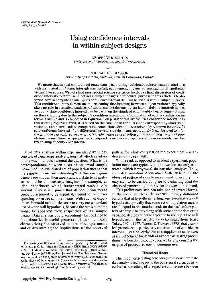
the population means increase with longer studytimes. In short, isolating the values of the individualpopulation means is generally interesting only insofaras it reveals something about the pattern that theyform.

6234 5Study Time per Word (sec)

(B) Between-Subjects CI: ±3.85

(A) Between Subjects Data

;..----: -

ANOVA

Source df SS MS F

Conditions 2 52.26 26.13 0.74

Within 27 953.60 35.32

Total 29 1005.86

30.,-----:---:---------::-,---------.,

o

30

25j~ 20Q)

II: 15E~ 10

'0 5Qj

~ 0:JZ

Within-Subject Data

Let us now suppose that the numbers from Table 1came not from a between-subject design, but from awithin-subject design. Suppose, that is, that the experi­ment included a total of n = 10 subjects, each of whomparticipated in all three study-time conditions. Table 2reproduces the Table 1 data from each of the three con­ditions, showing in addition the mean for each subject(row mean) along with the grand mean, M = 12.73(Table 2, bottom right). Figure 3 shows these data ingraphical form: the individual subject curves (thin lines)are shown along with the curve for the condition means(heavy line). Note that the condition means, based asthey are on the same numbers as they were in Table 1 andFigure 2, do not change.

(1)

138

142520174

171212

M 3 = 14.2

10 136 8

11 1422 2316 1815 17

1 112 159 \28 9

M, = 11.0 M 2 = 13.0

Note-MJ

= Mean ofConditionj

Between-Subject Confidence IntervalsFigure 2B shows the 95% confidence interval around

the three condition means. This confidence interval isbased on the pooled estimate ofthe within-condition vari­ance, that is, on MS w. It is therefore based on dfw= 27, andis computed by the usual formula,

JMSw ..CI =~ ± -n- [cntenon t(27)],

which, as indicated on the figure, is ±3.85 in this example.Figure 2B provides much the same information as

does the ANOVA shown in Figure 2A. In particular, aglance at Figure 2B indicates the same conclusionreached via the ANOVA: given our knowledge about thevalues of the three condition population means, we can'texclude the possibility that they are all equal. More gen­erally, the confidence intervals indicate that any possibleordering ofthe three population means is well within therealm of possibility. Note that the intimate correspon­dence between the ANOVA and the confidence intervalcomes about because their computations involve thecommon error term, MS w'

Figure 2. An example ofa between-subject design. Panel A: Meanssurrounded by individual data points. Panel B: Confidence intervalsaround the three data points.

Individual Population Means Versus PatternsofPopulation Means

A confidence interval, by definition, provides in­formation about the value of some specific populationmean; for example, the confidence interval aroundthe left-hand mean of Figure 2B provides informationabout the population mean corresponding to the l-seccondition. However, in psychological experiments, itis rare (although, as we discuss in a later section, notunknown) for one to be genuinely interested in infer­ring the specific value of a population mean. Moretypically, one is interested in inferring the patternformed by a set of population means. In the presentexample, the primary interest is not so much in theabsolute values of the three population means, butrather in how they are related to one another. A hy­pothesis that might be of interest, for example, is that

'C 25~iii 20~II: 15f1)

'E~ 10

'0 5

~E 0:JZ

o

t-i--1

2 3 4 5StUdy Time per Word (sec)

6

CONFIDENCE INTERVALS IN WITHIN-SUBJECT DESIGN 481

Exposure Duration Per Word

ure 2B (i.e., ±3.85). That is, if we wish to provide infor­mation about, say, the value of the I-sec-condition pop­ulation mean, we must construct the confidence intervalthat includes the same intersubject variability that con­stituted the error variance in the between-subject design.

Intuitively, this seems wrong. An immediately obvi­ous difficulty is that such a confidence interval wouldyield a conclusion different from that yielded by thewithin-subject ANOVA. We argued earlier that the Fig­ure 2B confidence interval shows graphically that wecould not make any strong inferences about the orderingof the three condition means (e.g., we could not rejectthe null hypothesis of no differences). In the between­subject example, this conclusion was entirely in accordwith the nonsignificant F yielded by the between-sub­ject ANOVA. In the within-subject counterpart, how­ever, such a conclusion would be entirely at odds withthe highly significant F yielded by the within-subjectANOVA. This conflict is no quirk; it occurs because theintersubject variance, which is irrelevant in the within­subject ANOVA, partially determines (and in this exam­ple would almost completely determine) the size of theconfidence interval. More generally, because the ANOVAand the confidence interval are based on different errorterms, they provide different (and seemingly conflicting)information.

A Within-Subject Confidence IntervalTo escape this conundrum, one can reason as follows.

Given the irrelevance of intersubject variance in awithin-subject design, it can legitimately be ignored forpurposes of statistical analysis. In Table 3 we have elim­inated intersubject variance without changing anythingelse. In Table 3, each of the three scores for a given sub­ject has been normalized by subtracting from the origi­nal (Table 2) score a subject-deviation score consistingof that subject's mean, M, (rightmost column ofTable 2)minus the grand mean, M = 12.73 (Table 2, bottom right).Thus, each subject's pattern of scores over the three con­ditions remains unchanged, and in addition the threecondition means remain unchanged. But, as is evident inTable 3, rightmost column, each subject has the samenormalized mean, equal to 12.73, the grand mean.

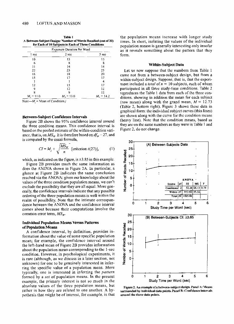
Figure 4 shows the data from Table 3; it is the Figure 3data minus the subject variability. As shown in Appen­dix A(3), there are now only two sources ofvariability inthe data: the condition variance is, as usual, reflected bythe differences among the three condition means, whilethe remaining variance-the interaction variance-is re­flected by the variability of points around each of thethree means.

Figure 5A shows the Figure 4 data redrawn with theindividual-subject curves removed, leaving only themean curve and the individual data points. It is evidentthat there is an intimate correspondence between Fig­ure 5A and Figure 2A. In both cases, the condition meansare shown surrounded by the individual data points, andin both cases the variability of the individual pointsaround the condition means represents the error vari-

6

Within-Subjects

Interaction 18 11.07 0.61

Total 29 1005.86

.......­.--' ...-._.-~----~---_..- --......

• 0-"'-

................................... ,_ ...._... ~ ----_._._-=.~.=-~-=-=;== .. =-.---

~~~~;:~=~~~~-- ANOVA

Source de ss MS F..•.........._- Conditions 2 52.27 26.13 42.51

Subjects 9 942.53 104.73

o

30~--------------~

"C 25Q)

'iij 20~a: 15lIJ'E~ 10

'0 5Qj.cE 0::JZ

Table 2A Within-Subject Design: Number RecaUed (out of20)

for 10 SUbjects in Each of Three Conditions

Subject 1 sec 2 sec 5 sec M,

I 10 13 13 12.002 6 8 8 7.333 11 14 14 13.004 22 23 25 23.335 16 18 20 18.006 15 17 17 16.337 1 1 4 2.008 12 15 17 14.679 9 12 12 11.00

10 8 9 12 9.67

MJ

M1 = 11.0 M 2 = 13.0 M 3 = 14.2 M = 12.73

Note-s-Each row corresponds to 1 subject. At; = mean of Condition};M, = mean of Subject i).

Error Variance and the Notion of"Consistency"The Figure 3 data pattern should suffice to convince

the reader that an effect of study time can be reasonablyinferred (specifically, a monotonically increasing rela­tion between study time and performance). This is be­cause each of the 10 subj ects shows a small but consis­tent study-time effect. Statistically, this consistency isreflected in the small mean square due to interaction(MSsxc = 0.61) in the ANOVA table at the bottom rightof Figure 3. And, indeed, the F for the study-time con­ditions, now computed as MSc/MSsxc is highly signifi­cant [F(2,18) = 42.51).

Constructing a Confidence IntervalSuppose that we wished to construct a confidence in­

terval based on these within-subject data. As shown inAppendix A(2), a bona fide confidence interval-one de­signed to provide information about values of individualpopulation means-would be exactly that shown in Fig-

2 3 4 5Study Time per Word (sec)

Figure 3. An example of a within-subject design. Means (connectedby the heavy solid line) are shown with individual subject curves(other lines).

482 LOFTUS AND MASSON

Subject Variability Removed30-r-----------------,

'C 25Q)

~ 20

/£(Jl 15'E~ 10

'0 5.!E 0::::lZ

val, in the sense that it does not provide information aboutthe value ofsome relevant population mean. Wehave alsonoted that in either a between- or a within-subject design,a bona fide confidence interval-one truly designed toprovide information about a population mean's value­must be based on intersubject variance as well as interac­tion variance. However,this Figure 5B confidence intervalhas an important property that justifies its use in a typicalwithin-subject design. This property has to do with infer­ring patterns ofpopulation means across conditions.

Earlier, we argued that a psychologist is typically in­terested not in the specific values of relevant populationmeans but in the pattern ofpopulation means across con­ditions. In the present hypothetical study, for example, itmight, as noted, be of interest to confirm a hypothesisthat the three-condition-population means form a mo­notonically increasing sequence.

In a within-subject design, as in a between-subject de­sign, an ANOVA is designed to address the question:Are there any differences among the population means?The within-subject confidence interval addresses thesame question. In its simplest form, the question boilsdown to: Are two sample means significantly different?In a between-subject design, there is a precise correspon­dence between the results of an ANOVA and the resultsof using confidence intervals:As shown in AppendixA(1),two sample means, M, and Mk , are significantly differentgiven a particular a if and only if

1~-Mkl>V2xCI,

where CI is the [100 (1.0 - a)]% confidence interval.As demonstrated in Appendix A(3), the within-subjectconfidence interval also has the property that it is relatedby a factor of V2 to the confidence interval around thedifference between two means.

In summary, a between-subject and a within-subjectconfidence interval function similarly in two ways. First,they both provide information that is consistent with that

ance used to test for the condition effect in the ANOVA.Intuitively, therefore, it is sensible to compute from theFigure 5A data something very much like the between­subject confidence interval that was computed from theFigure 2A data (cf. Figure 2B). Because the variabilityin Figure 5A is entirely interaction variance, the appro­priate formula is, as shown in Appendix A(3),

CI=~ ± J M:xc [criterion t(18)],

which, in this example, is ±0.52. More generally,

CI=~±JM:xc [criteriont(d.fsxd]. (2)

Thus, Equation 2 embodies a within-subject confidenceinterval. Note that there are two differences betweenEquations I and 2. First, the "error variance" in Equa­tion 2 is the interaction mean squares rather than thewithin mean squares. Second, the criterion t in Equa­tion 2 is based on d.fsxc rather than dfw.

Figure 5B shows the resulting confidence intervalsaround the three condition means. It is abundantly clearthat the information conveyed by Figure 5B mirrors theresult ofthe ANOVA, clearly implying differences amongthe population means. (To illustrate this clarity a fortiori,the small plot embedded in Figure 5B shows the samedata with the ordinate appropriately rescaled.) We em­phasize that this confidence interval and the associatedANOVA now provide concordant information becausethey are based on the same error term (MSsxd- just asin a between-subject design, the ANOVA and a confi­dence interval provide concordant information becausethey are both based on the same error term, MS w'

Subject I sec 2 sec 5 sec Mj = M

I 10.73 13.73 13.73 12.732 11.40 13.40 13.40 12.733 10.73 13.73 13.73 12.734 11.40 12.40 14.40 12.735 10.73 12.73 14.73 12.736 11.40 13.40 13.40 12.737 11.73 11.73 14.73 12.738 10.07 13.07 15.07 12.739 10.73 13.73 13.73 12.73

10 11.07 12.07 15.Q7 12.73

MJ

M, = 11.0 M1 = 13.0 M) = 14.2 M = 12.73

Note-Each subject's deviation score from the grand mean has beensubtracted from each subject's score. Condition means (M) do notchange from the Table 2 data.

Exposure Duration Per Word

Table 3Within-Subject Design: Data Nonnalized

to Remove Subject Variablity

INFERENCES ABOUT PATTERNSOF POPULATION MEANS o 1 2 3 4 5

StUdy Time per Word (sec)6

As we have noted, the "confidence interval" gener­ated by Equation 2 is not a bona fide confidence inter-

Figure 4. Subject variability has been removed from the Figure 2data using the procedure described in the text.

CONFIDENCE INTERVALS IN WITHIN-SUBJECT DESIGN 483

ADDITIONAL ISSUES

Figure 5. Construction of a within-subject confidence interval.Panel A: The only remaining variance is interaction variance.Panel B: A confidence interval constructed on the basis of the data inPanel A. Note the analogy between this figure and Figure 1.

The foregoing constitutes the major thrust of our re­marks. In this section, we address a number of other is­sues involving the use ofconfidence intervals in generaland within-subject confidence intervals in particular.

provided by the ANOVA, and second, they both providea clear, direct picture of the (presumably important) un­derlying pattern of population means. In addition, theyboth provide a clear, direct picture of relevant statisticalpower in that the smaller the confidence interval, thegreater the power.

In repeated measures ANOVAs applied to cases inwhich there are more than two conditions, the computedF ratio is, strictly speaking, correct only under the assump­tion ofsphericity. A strict form of sphericity (called com­pound symmetry) requires that population variances forall conditions be equal (homogeneity of variance) andthat the correlations between each pair of conditions beequal (homogeneity of covariance). If the sphericity as­sumption is violated (and it is arguable that this typicallyis the case; see, e.g., O'Brien & Kaiser, 1985), two prob­lems arise. First, the F ratio for the test of the conditionseffect tends to be inflated (Box, 1954). Corrections forthis problem have been developed in which the degreesof freedom used to test the obtained F ratio are adjustedaccording to the seriousness of the departure fromsphericity (Greenhouse & Geisser, 1959; Huynh &Feldt, 1976).

Second, violation of the sphericity assumption com­promises the use of the omnibus error term (and its as­sociated degrees of freedom) when testing planned orother types of contrasts. The omnibus error term is theaverage of the error terms associated with all possible1 df contrasts that could be performed with the set ofconditions that were tested. When sphericity is violated,these specific error terms may vary widely, so the om­nibus error term is not necessarily a valid estimate ofthe error term for a particular contrast (O'Brien &Kaiser, 1985).

One solution to the problem ofviolation ofthe spheric­ity assumption is to conduct a multivariate analysis ofvariance (MANOVA) in place of a univariate analysis ofvariance, an approach that some advocate as a generalsolution (e.g., O'Brien & Kaiser, 1985).The MANOVAtestavoids the problem of sphericity because it does not usepooled error terms. Instead, MANOVA is a multivariatetest of a set of orthogonal, 1 dfcontrasts, with each con­trast treated as a separate variable (not pooled as inANOVA).

The use ofMANOVAin place ofANOVA for repeatedmeasures designs is not, however, universally recom­mended. For example, Hertzog and Rovine (1985) rec­ommend estimating violations ofsphericity using the mea­sure e as an aid in deciding whether to use MANOVA inplace of ANOVA (e.g., Huynh & Feldt, 1970). Huynhand Feldt point out that such violations do not substan­tially influence the Type I error rate associated with uni­variate F tests unless e is less than about 0.75. For val­ues of e between 0.90 and 0.75, Hertzog and Rovinerecommend using the F tests with adjusted degrees offreedom, and only for values of e below 0.75 do theysuggest using MANOVA.

More important for our purposes is that the sphericityassumption problem arises only when considering om­nibus tests. As soon as one considers specific, 1 dfcon­trasts, as is often done after MANOVA is applied, thesphericity assumption is no longer in effect. Thus, a vi­able solution is to use the appropriate specific error termfor each contrast (e.g., Boik, 1981) and avoid thesphericity assumption altogether.

6

6

2 3 4 5Study Time per Word (sec)

2 3 4 5Study Time per Word (sec)

(A) Interaction Variance Around Means

(B) Within Subjects CI: ±0.52

-i

~ j 15

.:g14II:

~ 13

~ 12

Jlli 10

Study~m. ~rWool (~)

30.,....-----------------,

25'tJQ)

'iii 20~a: 15

~ ~~ 10

'0 5

~E 0:::JZ

o

25

o

'tJ 20~

~ 15Q)

a:~ 10

~ 5'0

~ 0E:::JZ

Assumptions

In our discussions thus far, we have made the usual as­sumptions (see Appendix A for a description of them).In this section, we discuss several issues regarding ef­fects of, and suggested procedures to be used in theevent of, assumption violations.

484 LOFTUS AND MASSON

The problems that result from violation of sphericityhave implications for the implementation of confidenceintervals as graphic aids and as alternatives to hypothe­sis testing. The computation of the confidence intervalas shown in Equation 2 uses the omnibus error term andis the interval that would be plotted with each mean, asin Figure 5. Given that a crucial function served by theplotted confidence interval is to provide an impressionof the pattern of differences among means, we must besensitive to the possibility that violation of sphericitycauses an underestimate of the interval's size.

To counteract the underestimation stemming from in­appropriately high degrees of freedom, one could use theGreenhouse-Geisser or Huynh-Feldt procedure (as com­puted by such ANOVA packages as BMDP) to adjust thedegrees of freedom used in establishing the criteriont value.

It is important to note that although the confidence in­terval computed by applying the adjustment to degreesoffreedom may be used to provide a general sense ofthepattern ofmeans, more specific questions about pairs ofmeans should be handled differently. If the omnibuserror term is not appropriate for use in contrasts whensphericity is violated, then the confidence interval plot­ted with each mean should be based on a specific errorterm. The choice of the error term to use will depend onthe contrast that is of interest. For example, in Figure 5it might be important to contrast the first and second du­ration conditions and the second and third conditions.The confidence interval plotted with the means of thefirst and second conditions would be based on the errorterm for contrasting 'those two conditions. The confi­dence interval plotted with the mean for the third condi­tion would be based on the error term for the contrast be­tween the second and third conditions. For ease ofcomparison, one might plot both intervals, side by Side,around the mean for the second condition. The choice ofwhich interval(s) to plot will depend on the primarymessage that the graph is intended to convey. Below, weprovide a specific example of plotting multiply derivedconfidence intervals to illustrate different characteris­tics of the data.

Another means of treating violation of the homo­geneity of variance assumption is to compute separateconfidence intervals for the separate condition means. Ina between-subject design, this is a simple procedure: oneestimates the population variance for each group.j (MSwjbased on nj - I dj, where nj is the number o~ obser~a­

tions in Group j), and then computes the confidence m­terval for that group as

JMSwCI = __1 X [criterion u», - I)].} n

j

An analogous procedure for a within-subject design isdescribed in Appendix B. The general idea underlyingthis procedure is that one allows the subject X conditioninteraction variance to differ from condition to condi­tion; the confidence interval for Condition j is then basedprimarily on the interaction variance from Conditionj.

The equation for computing the best estimate of thisCondition j interaction variance ("estimator/') is,

estimatorj = (J~ 1)(MS~ - MSJXC}

Here, MSsxc is the overall mean square due to interac­tion, and

~ 2 ~ 2 2MSfv = £..(yij-M) z.», -Tjln

J n-I n-I

(where T is the Group j total and again n is the numberofsubjedts). Thus, MS~ is the "mean square within" ob­tained from ConditionJof the normalized (Y~) scores(e.g., in this article's example, a mean square within agiven column ofTable 3). Having computed the estima­tor, the Group j confidence interval is computed as

estimator.C~ = } X criterion t(n - I). (3)

n

Mean Differences

Above, we discussed the relationship between confi­dence intervals around sample means and around thedifference between two sample means. Because this re­lation is the same (involving a factor ofy2) for both thebetween- and the within-subject confidence intervals,one could convey the same information in a plot by sim­ply including a single confidence interval appropriatefor the difference between two sample means.

Which type ofconfidence interval is preferable is partlya matter of taste, but also a matter of the questions beingaddressed in the experiment. Our examples in this arti­cle involved parametric experiments in which an entirepattern ofmeans was at issue. In our hypothetical experi­ments, one might ask, for instance, whether the relationbetween study time and performance is monotonic, orperhaps whether it conforms to some more specific under­lying mathematical function, such as an exponential ap­proach to an asymptote. In other experiments, morequalitative questions are addressed (e.g., What are therelations among conditions involving a positive, neutral,or negative prime?). Here, the focus would be on specificcomparisons between sample means, and a confidenceinterval of mean differences might be more useful.

Multifactor Designs

The logic that we have presented here is based on asimple design in which there is only a single factor thatis manipulated within subjects. In many experiments,however, there are two or more factors. In such cases, allfactors may be manipulated within subjects or some fac­tors may be within subjects while others are betweensubjects.

Multifactor Within-Subject DesignsConsider a design in which there are two fixed fac­

tors, A and B, with J and K levels per factor, combinedwith n subjects. In such a design, there are three error

CONFIDENCE INTERVALS IN WITHIN-SUBJECT DESIGN 485

(4)

terms, corresponding to the interactions of subjects withfactors A, B, and the A X B interaction. Roughly speak­ing, one of two basic results can occur in this design: ei­ther the three error terms are all approximately equal orthey differ substantially from one another.

As discussed in any standard design text (e.g., Winer,1971), when the error terms are all roughly equal, theycan be pooled by dividing the sum of the three sums ofsquares by the sum of the three degrees of freedom(which amounts to treating the design as if it were a sin­gle-factor design with JK conditions). A single confi­dence interval can then be computed using Equation 2,

JMSS X AB ..CI = M± .[en tenon t(dls x AB)]'} n

where S X AB refers to the interaction of subjects withthe combined JK conditions formed by combining fac­tors A and B [based on (n - I) (JK - I) degrees of free­dom]. This confidence interval is appropriate for com­paring any two means (or any pattern ofmeans) with oneanother.

As discussed above, the use ofthe omnibus error termdepends on meeting the sphericity assumption. Whenthis assumption is untenable (as indicated, for example,by a low value of £ computed in conjunction with theGreenhouse-Geisser or Huynh-Feldt procedure for cor­rected degrees of freedom or by substantially differenterror terms for main effects and interactions involvingthe repeated measures factors), different mean differ­ences are distributed with different variances, as shownin Appendix A(4). For instance, the standard error ap­propriate for assessing (~k - ~r) may be differentfrom that appropriate for assessing (Mj k - Mqk ) or(~k - M qr ) · In such cases, one should adopt the strategyof plotting confidence intervals that can be used to as­sess patterns of means or contrasts that are of greatestinterest. One might even plot more than one confidenceinterval for some means, or construct more than one plotfor the data. Finally, one could treat the design as a one­way design with "conditions" actually encompassing allJ X K cells; one could then drop the homogeneity-of­variance assumption and compute an individual confi­dence interval for each condition, as discussed in theAssumptions section above (see Equation 3). Here theinteraction term would be MSSXAB described as part ofEquation 4.

Mixed DesignsOther designs involve one or more factors manipu­

lated within subjects in conjunction with one or morefactors manipulated between subjects. Here, matters arefurther complicated, as evaluation of the between-sub­ject effect is almost always based on an error term thatis different from that of the evaluation of the within-sub­ject or the interaction effects. Here again, one could, atbest, construct different confidence intervals, dependingon which mean differences are to be emphasized.

Data Reduction in Multifactor DesignsAn alternative to treating multi factor data as simply a

collection of (say) J X K means is to assume a modelthat implies some form of preliminary data reduction.Such data reduction can functionally reduce the numberof factors in the design (e.g., could reduce a two-fixed­factor design to a one-fixed-factor design).

An example. To illustrate, suppose that one were in­terested in slope differences between various types ofstimulus materials (e.g., digits, letters, words) in a Stern­berg (1966) memory-scanning task. One might design acompletely within-subject experiment in which J levelsof set size were factorially combined with K levels ofstimulus type and n subjects. If it were assumed that thefunction relating reaction time to set size was funda­mentally linear, one could compute a slope for each sub­ject, thereby functionally reducing the design to a one­factor (stimulus type), within-subject design in which"slope" was the dependent measure. Confidence inter­vals around mean slopes for each stimulus-type levelcould be constructed in the manner that we have de­scribed. Alternatively, if stimulus type were varied be­tween subjects, computing a slope for each subject wouldallow one to treat the design as a one-way, between­subject design (again with "slope" as the dependentmeasure), and standard between-subject confidence in­tervals could be computed.

Contrasts. The slope ofan assumed linear function is,of course, a special case of a one-degree-of-freedomcontrast by which a single dependent variable can becomputed from a J-level factor as

y = LjWj~'

where the M j are the means of the j levels and the wj(constrained such that LjWj = 0) are the weights corre­sponding to the contrast. Thus, the above examples canbe generalized to any case in which the effect of somefactor can be reasonably well specified.

The case ofa J X 2 design. One particular fairly com­mon situation bears special mention. When the crucialaspect of a multifactor design is the interaction betweentwo factors, and one of the factors has only two levels,the data can be reduced to a set of J difference scores.These difference scores can be plotted along with theconfidence interval computed from the error term for anANOVA of the difference scores. A plot of this kind ad­dresses whether the differences between means are dif­ferent, and provides an immediate sense of (1) whetheran interaction is present, and (2) the pattern of the inter­action. Such a plot can accompany the usual plot show­ing all condition means.

To illustrate the flexibility of this approach, considera semantic priming experiment in which subjects nametarget words that are preceded by either a semanticallyrelated or unrelated prime word. Prime relatedness isfactorially combined within subjects with the prime­target stimulus onset asynchrony (SOA), which, suppose,is 50, 100, 200, or 400 msec. Hypothetical response-

486 LOFTUS AND MASSON

Table 4Data (Reaction Times) from 6 Subjects in a Hypothetical Priming Experiment

50-msec SOA 100-msec SOA 200-msec SOA 400-msec SOA

Subject R U D R U D R U D R U D

I 450 462 12 460 482 22 460 497 37 480 507 272 510 492 -18 515 530 15 520 534 14 504 550 463 492 508 16 512 522 10 503 553 50 520 539 194 524 532 8 530 543 I3 517 546 29 503 553 505 420 409 -II 424 452 28 431 468 37 446 472 266 540 550 10 538 528 -10 552 575 23 562 598 36

lWj 489 492 3 497 510 13 497 529 32 503 537 34

Note-Four values of SOA are combined with two priming conditions (columns labeled R = primed; columns labeled U= unprimed); columns labeled D represent unprimed minus primed difference scores at each SOA level.

latency data from 6 subjects are shown in Table 4. Themean latency for each of the eight conditions is plottedin Figure 6A. Confidence intervals in Figure 6A arebased on the comparison between related and unrelated

560(A) ......Aelated Prime

~ 550 ........Unrelated Prime

III

S 540Ql

.§ 530I-

.§ 520'0III 510a:~ 500Ql

::E490

4800 100 200 300 400

SOA (ms)Q 50Q)III

(B)SQ) 40ol:~Q) 30

/v=i5iii 20Ei=l:

~ 10ltIQ)

a: 0l:ltIQ)

::E ·100 100 200 300 400

SOA (msec)

Figure 6. IDustration of multiple ways of plotting to demonstratedifferent aspects of the data. Panel A: Mean reaction time (RT) as afunction ofthe eight conditions. Confidence intervals at each stimu­lus onset asynchrony (SOA) levelis based on the 5-dferror term fromthe one-way, two-level (primed vs, unprimed) analysis of variance(ANOVA) done at that SOA level. Panel B: Mean (primed ­unprimed) RT difference. Confidence intervals are based on theS X Cerrorterm from the ANOVAofRT differences.

prime conditions within a particular SOA (i.e., on the5-df error terms stemming from individual two-levelone-way ANOYAs performed at each SOA level). Thisplot thus illuminates the degree to which priming effectsare reliable at the different SOAs.

Suppose that a further avenue of investigation re­volves around the degree to which priming effects differin magnitude across the SOAs. In ANOYA terms, thequestion would be: Is there a reliable interaction be­tween prime type and SOA? A standard 4 X 2 within­subject ANOYA applied to these data shows that the in­teraction is significant [F(3, 15) = 7.08, MSsxc =95.39]. The nature of the interaction can be displayed byplotting mean difference scores (which, for individualsubjects, are obtained by subtracting the latency in therelated prime condition from the latency in the unrelatedprime condition) as a function of SOA. These differencescores (representing priming effects) are included inTable 4, and the mean difference scores are plotted inFigure 6B. The confidence intervals in Figure 6B arebased on the MSsxc term for a one-factor repeated mea­sures ANOYA of the difference scores (MSsxc =190.78). (Note that, as with any difference score, theerror term in this ANOYA is twice the magnitude of thecorresponding error terms in the full, two-factorANOYA that generated the F ratio for the interaction.)The bottom panel of Figure 6 indicates that, indeed, re­liably different priming effects occurred at differentSOAs (consistent with the significant interaction ob­tained in the two-factor ANOYA), and also reflects therange of patterns that this interaction could assume.

Knowledge of Absolute Population Means

Central to our reasoning up to now is that knowledgeof absolute population means is not critical to the ques­tion being addressed. Although this is usually true, it isnot, of course, always true. For instance, one might becarrying out a memory experiment in which one was in­terested in whether performance in some condition dif­fered from a 50% chance level. In this case, the within­subject confidence interval that we have describedwould be inappropriate. If one were to use a confidenceinterval in this situation, it would be necessary to use theconfidence interval that included the between-subjectvariation that we removed in our examples.

CONFIDENCE INTERVALS IN WITHIN-SUBJECT DESIGN 487

Meta-Analysis

One advantage ofreporting the results ofANOVA andtables of means and standard deviations is that it makestasks associated with meta-analysis easier and more pre­cise. In cases in which an author relies on graphical de­pictions ofdata using confidence intervals, as describedhere, it would be helpful to include in the Results sectiona statement of the effect size associated with each maineffect, interaction, or other contrast of interest in the de­sign. This information is not typically included even inarticles that apply standard hypothesis testing tech­niques with ANOVA. All researchers would benefit ifboth the hypothesis testing method and the graphical ap­proach advocated here were supplemented by estimatesof effect size.

CONCLUSIONS:DATAANALYSIS AS ART, NOT ALGORITHM

In this article, we have tried to accomplish a specificgoal: to describe an appropriate and useful confidenceinterval to be used in within-subject designs that servesthe same functions as does a confidence interval in a be­tween-subject design. Although we have attempted tocover a variety of "ifs, ands, and buts" in our sugges­tions, we obviously cannot cover all of them. We wouldlike to conclude by underscoring our belief that each ex­periment constitutes its own data-analysis challenge inwhich (1) specific (often multiple) hypotheses are to beevaluated, (2) standard assumptions may (or may not) beviolated to varying degrees, and (3) certain sources ofvariance or covariance are more important than others.Given this uniqueness, it is almost self-evident that noone set of algorithmic rules can appropriately cover allpossible situations.

REFERENCES

ANDERSON, v., & McLEAN, R. A. (1974). Design ofexperiments: A re­alistic approach. New York: Marcel Dekkar.

BAKAN, D. (1966). The test of significance in psychological research.Psychological Bulletin, 66,423-437.

BAYES, 1. (1763). An essay towards solving a problem in the doctrine ofchances. Philosophical Transactionsofthe Royal Society, 53, 370-418.

BERGER, J. 0., & BERRY, D. A. (1988). Statistical analysis and the il­lusion of objectivity. American Scientist, 76, 159-165.

BOIK, R. J. (1981). A priori tests in repeated measures designs: Effectsof nonsphericity. Psychometrika, 46, 241-255.

Box, G. E. 1'.(1954). Some theorems on quadratic forms applied in thestudy of analysis of variance problems: II. Effect of inequality ofvariance and of correlation between errors in the two-way classifi­cation. Annals ofMathematical Statistics, 25, 484-498.

Box, G. E. P. (1986). An apology for ecumenism in statistics. In G. E. 1'..Box, 1. Leonard, & C.-F. Wu (Eds.), Scientific inference, dataanalysis, and robustness (pp. 51-84). New York: Academic Press.

Box, G. E. 1'.., & TIAO, G. C. (1973). Bayesian inference in statisticalanalysis. Reading, MA: Addison-Wesley.

CAMILLI, G. (1990). The test ofhomogeneity for 2 X 2 contingency ta­bles: A review of and some personal opinions on the controversy.Psychological Bulletin, 108, 135-145.

COHEN, J. (1990). Things I have learned (so far). American Psycholo­gist, 45, 1304-1312.

FISHER, R. A. (1925). Statistical methods for research workers. Edin­burgh: Oliver & Boyd.

FISHER, R. A. (1935). The logic of inductive inference. Journal oftheRoyal Statistical Society, 98, 39-54.

FISHER, R. A. (1947). The design of experiments. New York: HafnerPress.

FISHER, R. A. (1955). Statistical methods and scientific induction.Journal ofthe Royal Statistical Society, Series B, 17,69-78.

GIGERENZER, G., SWIJTlNK, Z., PORTER, T., DASTON, L., BEATTY, J" &KRUGER, L. (1989). The empire ofchance. Cambridge: CambridgeUniversity Press.

GREENHOUSE, S. W., & GEISSER, S. (1959). On methods in the analy­sis of profile data. Psychometrika, 24, 95-1 12.

HAYS, W.(1973). Statistics for the social sciences (2nd ed.). New York:Holt.

HERTZOG, C., & ROVINE, M. (1985). Repeated-measures analysis ofvariance in developmental research: Selected issues. Child Devel­opment, 56, 787-809.

HUYNH, H., & FELDT, L. S. (1970). Conditions under which mean squareratios in repeated measures designs have exact F distributions. Jour­nal ofthe American Statistical Association, 65, 1582-1589.

HUYNH, H., & FELDT, L. S. (1976). Estimation of the Box correctionfor degrees of freedom from sample data in the randomized blockand split plot designs. Journal ofEducational Statistics, 1, 69-82.

LEHMANN, E. L. (1993). The Fisher, Neyman-Pearson theories of test­ing hypotheses: One theory or two? Journal ofthe American Statis­tical Association, 88,1242-1249.

LEWIS, C. (1993). Bayesian methods for the analysis of variance. InG. Kerens & C. Lewis (Eds.), A handbookfor data analysis in thebehavioral sciences: Statistical issues (pp. 233-258). Hillsdale, NJ:Erlbaum.

LOFTUS, G. R. (1991). On the tyranny of hypothesis testing in the so­cial sciences. Contemporary Psychology, 36,102-105.

LOFTUS, G. R. (I 993a). Editorial Comment. Memory & Cognition, 21,1-3.

LOFTUS, G. R. (1993b, November). On the overreliance ofsignificancetesting in the social sciences. Paper presented at the annual meetingof the Psychonomic Society, Washington, DC.

LOFTUS, G. R. (I 993c). Visual data representation and hypothesis test­ing in the microcomputer age. Behavior Research Methods, Instru­mentation, & Computers, 25, 250-256.

LOFTUS, G. R., & LOFTUS, E. F. (1988). Essence ofstatistics (2nd ed.).New York: Random House.

NEYMAN, J. (1957). "Inductive behavior" as a basic concept of phil os­ophy of science. Review ofthe International Statistical Institute, 25,7-22.

NEYMAN, J., & PEARSON, E. S. (1928). On the use and interpretation ofcertain test criteria for purposes of statistical inference. Biometrika,20A, 175-240, 263-294.

NEYMAN, J., & PEARSON, E. S. (1933). On the problem of the most ef­ficient tests of statistical hypotheses. Philosophical Transactions ofthe Royal Society ofLondon, Series A, 231, 289-337.

O'BRIEN, R. G., & KAISER, M. K. (1985). MANOVA method for ana­lyzing repeated measures designs: An extensive primer. Psycholog­ical Bulletin, 97, 316-333.

STERNBERG, S. (1966). High-speed scanning in human memory. Sci­ence, 153, 652-654.

TuFTE, E. R. (1983). The visual display ofquantitative information.Cheshire, CT: Graphics Press.

TuFTE,E. R. (1990). Envisioning information. Cheshire, CT: GraphicsPress.

TuKEY, J. W. (1974). The future of data analysis. Annals of Mathe­matical Statistics, 33, 1-67.

TuKEY, J. W. (1977). Exploratory data analysis. Reading, MA: Addison­Wesley.

WAINER, H., & THISSEN, D. (1993). Graphical data analysis. InG. Kerens & C. Lewis (Eds.), A handbookfor data analysis in thebehavioral sciences: Statistical issues (pp. 391-458). Hillsdale, NJ:Erlbaum.

WINER, B. J. (1971). Statistical principles in experimental design(2nd ed.). New York: McGraw-Hill.

WINKLER, R. L. (1993). Bayesian statistics: An overview. In G. Kerens& C. Lewis (Eds.), A handbook for data analysis in the behavioralsciences: Statistical issues (pp, 201-232). Hillsdale, NJ: Erlbaum.

488 LOFTUS AND MASSON

where criterion t(dfw) is two-tailed at the 1OO( 1.0 - x)% level, or

~ .MSEj_k = V2 X ----;;--n- = V 2 X SEj .

(A3)

n

1M . -Mk I} > criterion t( dfw),

!2xMS w~

As above, Yij is the score obtained by Subject i in Condition},f.J. is the population mean, and aj is an effect of the Condition}treatment. Again, 'Yi is an effect due to Subject i (note that Iinow has only a single subscript, i, since each subject partici­pates in all conditions). Again, gij is the interaction effect ofSubject i's being in Condition). We make the same assump­tions about Ii and the gij as we did in the preceding section.

The mean of Condition}, Mj , has an expectation of

E(M;) = E[(l/n)LiCU + aj + Ii + gi)]

= E[f.J. + a j + I/nL;(1i + gi)]

= f.J. + a j + I/nLiE(Y;) + I/nLiE(gi)

or, because E( Y;)= E(gi) = 0 for all},

E(M;) = f.J. + aj = f.J.j' (M)

where f.J.j is the population mean given condition).

Therefore, the standard error of the mean and the standarderror of the difference between two means are related by yz.A corollary of this conclusion is that two means, M; and M k ,

are significantly different by a two-tailed t test at some signif­icance level, x, if and only if,

2. Within-8ubject DesignsNow consider a standard one-factor, within-subject design

in which n subjects from the population are assumed to be ran­domly sampled but each subject participates in all J condi­tions. Each subject thus contributes one observation to eachcondition. The linear model underlying the ANOVA is

IM-Mkl JMSwJ yz > -n- criterion t(dfw) = C/,

where C/ at the right of the equation refers to the 100(1.0­x)% confidence interval. Thus, as asserted in the text, M; andM; differ significantly at the x level when

1M; - Mkl > yz X C/.

embodied in Equation A2 and the assumptions that we havearticulated.

l , The expectation of Mj, the mean of Condition}, is f.J.i'where f.J.J' the population mean given Condition), is equal tof.J.+ aj'

2. An unbiased estimate of the error variance, ai, is pro­vided by MS wbased onJ(n - 1) df The condition means, Mj ,

are distributed over samples of size n with variance Q}ln. Thus,the standard error of Mj , SEJ' computed as yMSwln, is deter­mined by the same quantity (MS w) that constitutes the errorterm in the ANOVA.

3. The standard error of the difference between any twomeans, M; and Mk , is computed by

(A2)

NarES

I. For expositional simplicity, we will use sample means in our ar­guments, realizing that analogous argumentscould be made about anysample statistic.

2. Some caveats should be noted in conjunction with these asser­tions. First, on occasion, a plausible null hypothesis does exist (e.g.,that performanceis at chance in a parapsychological experiment).Sec­ond, in a two-tailed z- or r-test situation, rejection of some null hy­pothesis can establish the directionality of some effect. (Note, how­ever, that even this latter situation rests on a logic by which one teststhe validity of some usually implausiblenull hypothesis.)

3. Becauseweare interested in comparingwithin-and between-sub­ject designs, we restrict ourselves to between-subject situations inwhich equal numbers of subjects are assigned to all J conditions. Wealso assume homogeneity of variance, which implies that confidenceintervals around all sample means are determined by a common,poolederror term. In a later section,we consider the case in which thisassumption is dropped.

As is demonstrated in any standard statistics textbook (e.g.,Hays, 1973, chap. 12-13), the following is true given the model

APPENDIX A

We begin by considering a between-subject design, and pro­viding the logic underlying the computation of the usual stan­dard error of the mean. We then articulate the assumptions ofthe within-subject standard error, and demonstrate its relationto its between-subject counterpart. Our primary goal is to showthat the within-subject standard error plays the same role asdoes the standard, between-subject standard error in twosenses: its size is determined by the error term used in theANOVA; and it is related by a factor of yz to the standarderror of the difference between two means. Appendix sectionsare numbered for ease of reference in the text.

1. Between-Subject DesignsConsider a standard one-factor, between-subject design in

which subjects from some population are assumed to be ran­domly sampled and randomly assigned to one ofJ conditions.Each subject thus contributes one observation to one condition.All observations are independent of one another. Because weare primarily concerned with comparing between- with within­subject designs, we lose little generality by assuming that thereare equal numbers, n, of subjects in each of the J conditions.The fixed-effects linear model underlying the ANOVA is,

Yij = u + aj + Yij + gij' (AI)

Here, Yij is the score obtained by Subject i in Condition}, f.J. isthe grand population mean, aj is an effect of the Condition}treatment (Ljaj = 0), Yij is an effect due to Subject ij, and gijis an interaction effect of Subject ij's being in Condition). Weinclude both lij and gij for completeness although they cannot,of course, be separated in a between-subject design. We as­sume that the 'Yij are normally distributed over subjects in thepopulation with means ofzero and variances of a~. We assumethat the gij are likewise normally distributed over subjects inthe population with means of zero and variances of a~ for allJ conditions. We assume that for each condition,}, the lij andthe gij are independent and that the gij are independent of oneanother over conditions. Notationally, we let lij + gij = eii'which, given our assumptions so far, means that we can define"error variance," o], to be a~ + ai and that Equation 1 can berewritten as

CONFIDENCE INTERVALS IN WITHIN-SUBJECT DESIGN 489

The expectation of (Yij - M)2 is

E(Yij - My = E[(,uj + Yi + s., -lInLi(,uj + Yi + gi)P,

which reduces to

E(Yij - ~)2 = (a; + ai)[(n - l)/n]. (AS)

Thus, the variability of the Yij scores around ~ includes vari­ance both from subjects (Yi) and from interaction ss.,»

The variance of the ~s around,uj is

E(~ - ,uY = E[lInLi(,uj + Yi + gij - ,u)]2

= E[lInLi(Ji + gi)J2

= E[LiYr/n + Lg2/n], '1

= (a; + aD/no (A6)

That is, over random samples of subjects, the variability of the~s includes both subject and interaction variability. An unbi­ased estimate of(a; + ai)/n is obtained by (MSs + MSsxc)/n.Therefore,thebona fide standarderrorof~ isV(MSs + MSsxc)/n.

3. Removal oflntersubject VarianceWe now consider our proposed correction to each score de­

signed to remove subject variance (that resulted in the trans­formation from Table 2 to Table 3 in the text). This correctionconsisted of subtracting from each of Subject i's scores anamount equal to Subject i's over-condition mean, Mi , minusthe grand mean, M. Thus, the equation for the transformed de­pendent variable, y~, is

Y~ = ,u + a j + Ji + gij - M, + M. (A7)

It can easily be demonstrated that the transformed mean ofCondition), M;, equals the untransformed mean, M; A com­parison of Equations 3 and 7 indicates that M; and Mj differ bymean over the n subjects of (M - M i ) , or

M; - Mj = IInLi(M - M,) = M - IInLjl/JLiYij

= M - Un ) (JnM) = 0,

which means that Mj = M;. Therefore, by Equation 4, we con­clude that the expectation ofM;= Mj , the mean of Condition),is ,uj, the population mean given Condition).

Next, we consider the within-condition variance of the Y~

scores. The variance of the (Y~ - M) scores is

E(y~ - My = E(Yij - M, + M - ~)2

= E[,u + aj + Yi + gij

- (~)L/,u + aj + Yi + gi)

+ Un)LjLi(,u + aj + Yi + gi)

- (~)Li(,u + aj + Yi + giY'

which can be reduced to

E(y~ - ~)2 = a;[(n - l)/n].

Thus, the within-cell variance of the yij scores includes onlythe interaction component. Moreover, the only additional vari­ance of the Yij scores is variance due to conditions.

We have asserted in the text that the variance of the yijscores within each condition plays a role analogous to that ofthe variance of the individual subject scores within each con­dition of a between-subject design. More precisely, we con­sider a "sum of squares within" over the Yij scores, which canbe computed as

SS:V = LjL;(yij - ~)2 = LjLi(Y~ + M, - M - ~)2,

which reduces to

SS:V = LjLiYi] - JLiM? - nLj~2 + JnM2,

which is equal to sum of squares due to the subject X condi­tion interaction. This means that the variance of the yij scoreswithin each condition are distributed with a variance that canbe estimated by MSsxc, whose expectation is err Therefore,the standard error is computed by

SE = JMSsxcj n'

As in the between-subject case, accordingly, the size of thestandard error is determined by the same quantity (MSsxd thatconstitutes the error term in the ANOVA.

Now consider the difference between two sample means

(Mj - Mk) = (~ )Li (,uj + Yi + gi) - lInLi (,uk + Yi + Kk)

= ( ~)Li (,uj - ,uk+ s.,- gik)

= (,uj - ,uk) + (~ )Li(gij - s.,: (A8)

The gij and gik are assumed to be distributed independently,with means of zero; thus, the expectation of~ - M; is u, ­,uk'By the homogeneity of variance assumption, the gij andgikare distributed identically in Conditions) and k, with variancea;. The M, - M, are therefore distributed with a varianceequal to 2a;Jn, which, in turn, is estimated by 2MSsxc/n. Thisimplies that the standard deviation of the difference betweenany two means,~ and Mk , is

SE = J2 X MSsxc = 2 X SEj-k j'n

Therefore, the standard error is related to the standard error ofthe difference between two means by 2, just as it is in abetween-subject case.

4. MuItifactor DesignsConsider a J X K design in which each of n subjects partic­

ipates in each JK level. The model describing this situation is

Yij=,u + aj + f3k+ a~k + X + gijk + agij + bgik + abgijk' (A9)

Here, YiP,u, and aj are as in Equation A3, while a~k is an ef­fect due to the A X B interaction. The subject-by-cell interac­tion term gijkacts like gij in Equation A3, but has an extra sub­script to refer to all JK cells. The agij, the interaction ofsubjects with factor A sums to zero over the J levels ofA, andis identical at each level k for each subject, i. Likewise, thebgik, the interaction of subjects with factor B, sums to zeroover all K levels of B, and is identical at each level) for eachsubject, i. Finally, the abg ijk, the interaction of subjects withthe A X B interaction sum to zero both over all J levels of fac-

490 LOFTUS AND MASSON

or

[ai/n - I)(J - 2)] + [oi(n - I)]

J

(BI)

-2ag+--.J-2

Because the first factor in this Equation is MS~J'

E[MSrv (_J)] = 0'2. + u; .j l J -2 s, J-2

[a2(n - 1)(1- 2)] + [o2(n - I)]I _ 2 = gj g

E(~j Mj ) J

which means that the expectation of the mean square withinGroup j, MS~j' is

rL;( YiJ- M j )2]_ 2 (J-2] U;

E -a -- +-n-I s, J J '

Thus, the expectation ofthe sum of squares within the Y:j scoresof Groupj is

Across different rows within a column:

tor A for each level k and across all K levels of factor B for eachlevel}.

There are three mean squares involving subject interactions:the A X S, B X S, and A X B X S interactions, which are theANOYA error terms for the effects of A, B, and A X B. Asshown in any standard design text (e.g., Winer, 1971, chap. 7),the expected mean squares of each of these interactions(MS'XA' MSsxB,and MSsxAxB)contain both a a; and a a~ com­ponent along with another vanance component correspondingto the specific effect (a~, affi, etc.). If, using standard proce­dures, one can infer that aJg= a1;g = aJbg = 0, then, for makinginferences about the effects of A, B, or A X B, there remainsonly a single source of error, ai, which is estimated by thepooled variances due to A X S, B X S, and A X B X S.

We have been emphasizing that confidence intervals-bothstandard confidence intervals and the within-subject confi­dence intervals-are appropriate for assessing patterns ofmeans or, most basically, differences between means. Giventhe model in Equation A9, the standard error of the differencebetween two means depends on which two means are beingcompared. In particular, for comparisons,

Across different columns within a row:

E(SE}k_jr) =It can be shown that the expectation of the overall mean

square due to interaction MSsxc is u;. Therefore,

Across different rows and columns: i MSsxc )=ui .l J-2 J-2

(B2)

The standard errors appropriate for any arbitrary mean differ­ence will, accordingly, be equal only when aJg= a1;g = O.

APPENDIXB

In our previous considerations, we have made a homogeneity­of-variance assumption for the gij (interaction components).That is, we have assumed that a; is identical for each of the jconditions. We now drop this assumption, and assume that thevariance of the gij is aj. Denote the mean variance of the J ais(over the J conditions) as aj. J

Consider Group}. The variance ofthe gij for that group, ai,is estimated as follows. First, the expectation ofthe variance 6fthe normalized scores, Y~ is

E(Y:j - ~)2 = E(J.1 + aj + Y; + gij - M; + M)2,

which (after not inconsiderable algebra) reduces to

Substituting the left side ofEquation B2 for the rightmost termof Equation B I, and rearranging terms, the estimator of ail is

E[C~2J(MSW; - MS;xc )]=u~;, (B3)

as indicated in the text.There is one potential problem with the Equation B3 esti­

mator: Because it is the difference of two estimated variances,it can turn out to be negative. In such an instance, two possiblesolutions are (I) to use the overall estimator or (2) to averageestimates from multiple groups which, for some a priori rea­son, can be considered to have equal variances.

(Manuscript received December 6, 1993;revision accepted for publication July 29,1994.)