CONFIDENCE INTERVALS FOR IMPULSE RESPONSES FROM

VAR MODELS: A COMPARISON OF ASYMPTOTIC THEORY

AND SIMULATION APPROACHES

William Griffiths

and

Helmut L~tkepohl

No. 42 - March 1990

ISSN

ISBN

0157-0188

0 85834 870 5

Department of EconometricsUniversity of New EnglandARMIDALE NSW 2351

CONFIDENCE INTERVALS FOR IMPULSE RESPONSES FROM VARMODELS:

A COMPARISON OF ASYMPTOTIC THEORY AND SIMULATION APPROACHES

William Griffiths~

University of New England, Armidale, Australia.

and

Helmut LOtkepohl~

Christian-Albrechts-Universit~t, Kiel, West Germany

ABSTRACT

Impulse responses are standard too]s ~n applied work for analysing the

interrelationships between the variables of vector autoregressive (VAR)

models. Asymptotic theory or simulation and bootstrapping methods are usually

used for measuring the estimation variability of estimated impulse responses.

In this study the small sample properties of these different approaches are

compared in a Monte Carlo investigation. The results indicate that, in terms

of their actual level, confidence intervals based on asymptotic theory are at

least as good as confidence intervals obtained with simulation and

bootstrapping methods, even in situations where the asymptotic theory is used

incorrectly.

~ The authors would like to thank Wenfang Zhang for his efficient andenthusiastic research assistance. LNtkepohl acknowledges support from aUniversity Visiting Research Fellowship.

Address for correspondence: William E. Griffiths,EconometrJ.cs Department,University of New England,Armidale. N.S.W. 2351.Australia.

i. Introduction

In a seminal paper Sims (1980) criticized conventional macroeconometric

modelling procedures and proposed an alternative strategy based on vector

autoregressive (VAR) models. Since that time the VAR approach has been widely

used in applied work. Important information provided by a VAR model is the

set of impulse response coefficients. Usually it is difficult, if not

impossible, to directly interpret the coefficients of an estimated VAR model.

Thus, impulse responses are often computed in order to study the

interrelationships within the variables of a system.

The impulse responses represent the reactions of the system to exogenous

shocks. They are functions of the VAR parameters and are estimated

accordingly. Different approaches have been used to measure the sampling

variability of the resulting estimators. One possibility is to employ

standard asymptotic theory and use the asymptotic distribution to compute

standard errors, t-ratios or confidence intervals for the impulse responses.

Alternatively, bootstrap and simulation methods have been used for that

purpose. Yet, little seems to be known ~bout the relative merits of these

different procedures. Some results on this question are provided in this

paper. Confidence intervals for the impulse responses, based on asymptotic

theory and on different simulation and bootstrap type procedures, are compared

on the basis of their finite sample accuracy.

The plan of the paper is as follows. In the next section the general

framework is laid out and the different methods for obtaining confidence

intervals for the impulse responses are described. In Section 3 the details

of the Monte Carlo experiment are given; the results are discussed in

Section 4, followed by conclusions in Section 5.

2. The General Framework

2.1 VAR Processes and Impulse Responses

Suppose a set of K variables Yt = (Ylt ..... YKt)’ is generated by a

VAR(p) process of the form

Yt- ~ = AI(Yt-I - ~) + "’" + Ap(Yt-P- R) + ut’ (2.1)

where ~ = (~I ..... ~K)’ is the (K × I) mean vector of the process, the Ai

are (K × K) coefficient matrices and ut = (Ult ..... UKt)’ is zero meanK-dimenslonal white noise with nonsingular covariance matrix Zu = E(utu[).

Alternative forms of impulse responses have been considered in VAR

analyses. Some authors prefer the responses of the system to forecast errors

whereas others consider the responses to orthogonalised or uncorrelated

residuals. The former may be obtained recursively from

~’i = [¢k~,i]k,£ = @i(AI’’’’’Ap) = j=1~i_jZ A~,o i = 1,2,...,(2.2)

where @0 = IK, Aj = 0 for j > p and ¢k£,i is the k~-th element of ~.,l

represents the response of variable k to a one unit forecast error or

and

residual in variable 6, i periods ago, providing no other shocks contaminate

the system (e g. LNtkepohl (1990)). The notation ~.(A1 ....A ) is used to¯ ’ 1 ’p

indicate that the impulse responses are functions of the VAR coefficients.

The responses to orthogonalised res|duals may be obtained as

®i = [8k~,i]k,~ = @i(Al ..... Ap, Eu) = ~iP, i = 0, I,...,(2.3)

where P is a lower triangular matrix with positive diagonal elements

satisfying PP’ = Z .u

In other words, P is determined by a Choleski

decomposition of Zu. The k~-th element of ®.~, 8k£, i’ is interpreted as the

response of variable k to an impulse in variable ~ one residual standard

deviation in magnitude, i periods ago. The � and 8 impulse responses are the

quantities of interest in the following.

2.2 Estimation of the VAR Coefficients and Impulse Responses

Suppose a sample of size T, Yl ..... YT’ and p presample values are

available for estimating the VAR(p) process (2.1). The sample mean

Ty = E Yt/T is often used as an estimator for the mean vector ~ and the

t=lare usually estimated by multivariate leastcoefficients ~ = [A1 ..... Ap]

squares (LS) or by Yule-Walker estimation, and sometimes Bayesian restrictions

are imposed. We use the LS estimator for ~ based on mean adjusted data,

A = YX’(XX’) ,(2.4)

where

y = [yl-~ ..... yT-~] and X = [X0 ..... XT_I] with Xt =

(KxT) (Kp:<T)

(Kpxl)

If the process is Gaussian with ut ~ N(O, Zu) this is the maximum

likelihood (ML) estimator conditional on the presample values. In small

samples it differs slightly from the Yule-Walker estimator. Our estimator for

E isU ^

m = (Y - ~XI(Y - AX)’/T.(2.5)

and O of theUsing these estimators in (2.2) and (2.3) gives estimators ~i i

impulse responses.

For a stationary Gaussian process the estimators are consistent and

asymptotically normally distributed,

’vec(~--A) ] d > N [0’

vech (~u-Zu)]

E 0

(2.6)

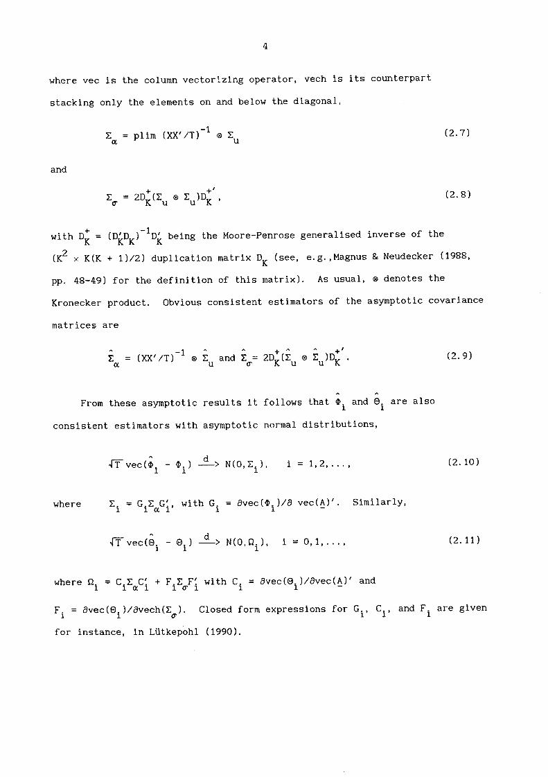
4

where vec is the column vectorizing operator, vech is its counterpart

stacking only the elements on and below the diagonal,

Z = plim (XX’/T)-I- ® Z (2.7)u

and

+Zo" = 2DK(Zu ® Zu)DK , (2.8)

being+ (DKDK)-ID~ the Moore-Penrose generalised inverse of thewith DK =

(K2 × K(K + 1)/2) duplication matrix DK (see, e.g.,Magnus & Neudecker (1988,

pp. 48-49) for the definition of this matrix). As usual, ® denotes the

Kronecker product. Obvious consistent estimators of the asymptotic covariance

matrices are

^ ^ ^ + ^ ^ +I

Z = (XX’/T)-1 ® Z and Z~=

2DK(Zu ® Z )DK .

~ U U(2.9)

^

From these asymptotic results it follows that ~. and ®. are also1 1

consistent estimators with asymptotic normal distributions,

4-~-vec(~i _ ~i) d> N(O,Zi), i = 1,z ..... (2.10)

where Z = GiZaG~ ¢i "i , with Gi = Ovec( )/0 vec(A)’_ Similarly,

--^IT vec(8. - 8.) d > N(O ~i) i : 0, I ....1 1 ’ ’ ’(2.11)

where ~. = C.Z C: + F.Z F’. with C. = 8vec(8.)/Ovec(A)’ and1 1 (X 1 1 (Y 1 1 1 -

Fi = Ovec(Si)/Ovech(Z¢). Closed form expressions for Gi, Ci, and F.1 are given

for instance, in Lfitkepohl (1990).

Consistent estimators of the covariance matrices are obtained by

replacing all unknown quantities with the estimators described in the

foregoing¯ These estimators may be used in the usual way to obtain "t-ratios"

and confidence intervals for the individual coefficients. It should be noted,

however, that Zi and ~’i may be singular with zero elements on the diagonal.

For instance, if Yt is actually a VAR(O) white noise process and a VAR(1)

process is fitted, Zi = 0 for i = 2,3 ..... In such a case the corresponding

parameter estimators converge to their actual values more rapidly than at the

usual 4-~--rate and the usual "t-ratios" wl]l in general not have an asymptotic

standard normal distribution. Under these circumstances the actual confidence

level of confidence intervals from (2.10) and (2¯11) may be different from the

assumed level.

The asymptotic results given here hold for stationary processes. In

their general form they also remain valid for cointegrated processes (see Park

and Phillips (1989)) The covariance matrix Z will be different from (2.7)¯ ~

in this case. However, the estimator given in (2.9) remains a consistent

estimator for Z . Hence, from a practical point of view we may proceed as in

the stationary case,

An alternative asymptotic theory exists that can be used if the VAR order

is unknown and potentially infinite. That theory proceeds on the assumption

that the order of the process fitted to the data goes to infinity with the

sample size (e.g., LGtkepohl, (1988)). As a result of the Monte Carlo setup

used in the present study such an assumption is not reasonable here and is

therefore not given further consideration.

2.3 Simulation Approaches

As alternatives to the use of asymptotic theory for the construction of

impulse-response confidence intervals, simulation and bootstrapping procedures

6

are often used. The motivation for using such procedures is the belief that,

in finite samples that are not large, they will provide a more accurate

assessment of estimator reliability. Also, although the general asymptotic

theory is valid for nonnormal processes, its performance many deteriorate if

the process distribution is markedly different from the normal. Moreover, the

asymptotic distribution of the orthogonal (8) impulse responses depends on the

process distribution because Z~, the asymptotic covariance matrix of the^

depends on that distribution. If the process distribution iselements of Zu,

unknown and nonnormal and one proceeds under an incorrect assumption that the

process is normal and thus uses the incorrect asymptotic distribution of the 8

impulse-responses, we might expect bootstrap methods that are based on the

empirical distribution of the residuals to have an advantage.

To use simulation or bootstrapping methods we proceed with the following

steps.

Step I: Given a sample of size T plus p presample values compute the LS/ML

estimators A and Z

Step 2: Generate N sets of residuals U(n) = [ul(n),...,uT(n)], n = 1 ..... N,

and, based on these residuals, generate new samples

^

Yt(n) = y + _A + ut(n), t = 1 ..... T.

Step 3: For each generated sample determine ~(n) and LS estimators ~(n),_^

^

Zu(n) and the corresponding impulse response estimates ~i(n) and ®i(n).

Step 4: From the resulting empirical distributions of the impulse responses

a) determine the empirical standard deviations and set up confidence

intervals with quantiles from a normal distribution table; or

7

b) determine the empirical quantiles and use them to set up confidence

intervals.

In Step 2 we use two different ways to generate residuals. The first

possibility is to draw the ut(n) from a multivariate N(0, ~u) distribution

whereas the second possibility is to draw randomly, with replacement, from the^ ^ ^ ^

LS residuals U = [uI .... ,uT] = Y - AX._ In the following the latter approach

will be referred to as bootstrapping and the former is called simulation with

normal residuals.

In total we have described five different methods to set up confidence

intervals for individual impulse response coefficients. We will number them

as follows:

I - based on asymptotic theory,

2 - based on standard errors obtained from simulation with normal

residuals,

3 - based on empirical quantiles obtained from simulation with normal

residuals,

4 - based on standard errors obtained from bootstrapping,

5 - based on empirical quantiles obtained from bootstrapping.

3. The Monte Carlo Setup

The finite sample accuracies of the five confidence interval methods were

evaluated within the framework of a Monte Carlo study. In a study of this

type the number of alternative setups is enormous. Choices have to be made

concerning the dimension and order of the VAR process, the settings for ~, AI,

A2 .... A and Zu, the error distribution, whether the order of the VAR process’ p

is assumed known or estimated, the sample size T, the number of simulations

(N) for the simulation techniques, and the number of replications.

Furthermore, the computational task is immense in a Monte Carlo experiment

8

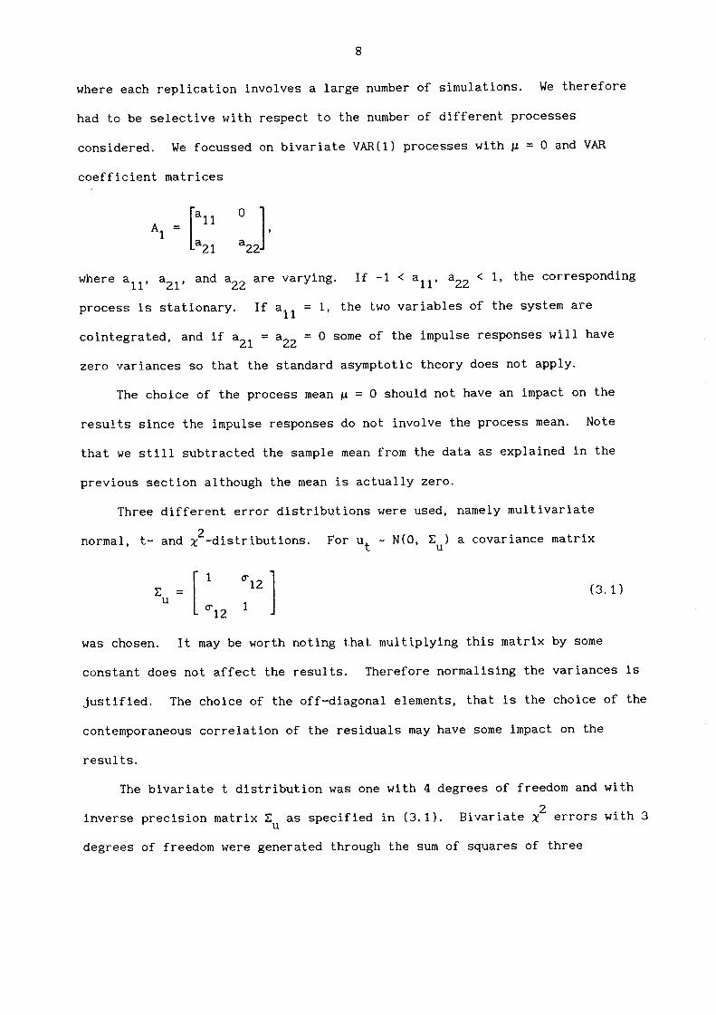
where each replication involves a large number of simulations. We therefore

had to be selective with respect to the number of different processes

considered. We focussed on bivariate VAR(i) processes with ~ = 0 and VAR

coefficient matrices

Iall 0 ]

A1 =,

[a21 a22

where all, a21, and a22 are varying. If -1 < a11, a22 < 1, the corresponding

process is stationary. If all = 1, the two variables of the system are

cofntegrated, and if a21 = a22 = 0 some of the impulse responses will have

zero variances so that the standard asymptotic theory does not apply.

The choice of the process mean g = 0 should not have an impact on the

results since the impulse responses do not involve the process mean. Note

that we still subtracted the sample mean from the data as explained in the

previous section although the mean is actually zero.

Three different error distributions were used, namely multivariate

normal, t- and ~2-distributions.

1 ~12 ]~u = 1

~12

For ut N N(0, Zu) a covariance matrix

was chosen. It may be worth noting that multiplying this matrix by some

(3.1)

contemporaneous correlation of the residuals may have some impact on the

results.

The bivariate t distribution was one with 4 degrees of freedom and with

inverse precision matrix ~ as specified in (3.1).u

2Bivariate 5~ errors with 3

degrees of freedom were generated through the sum of squares of three

justified. The choice of the off-diagonal elements, that is the choice of the

constant does not affect the results. Therefore normalising the variances is

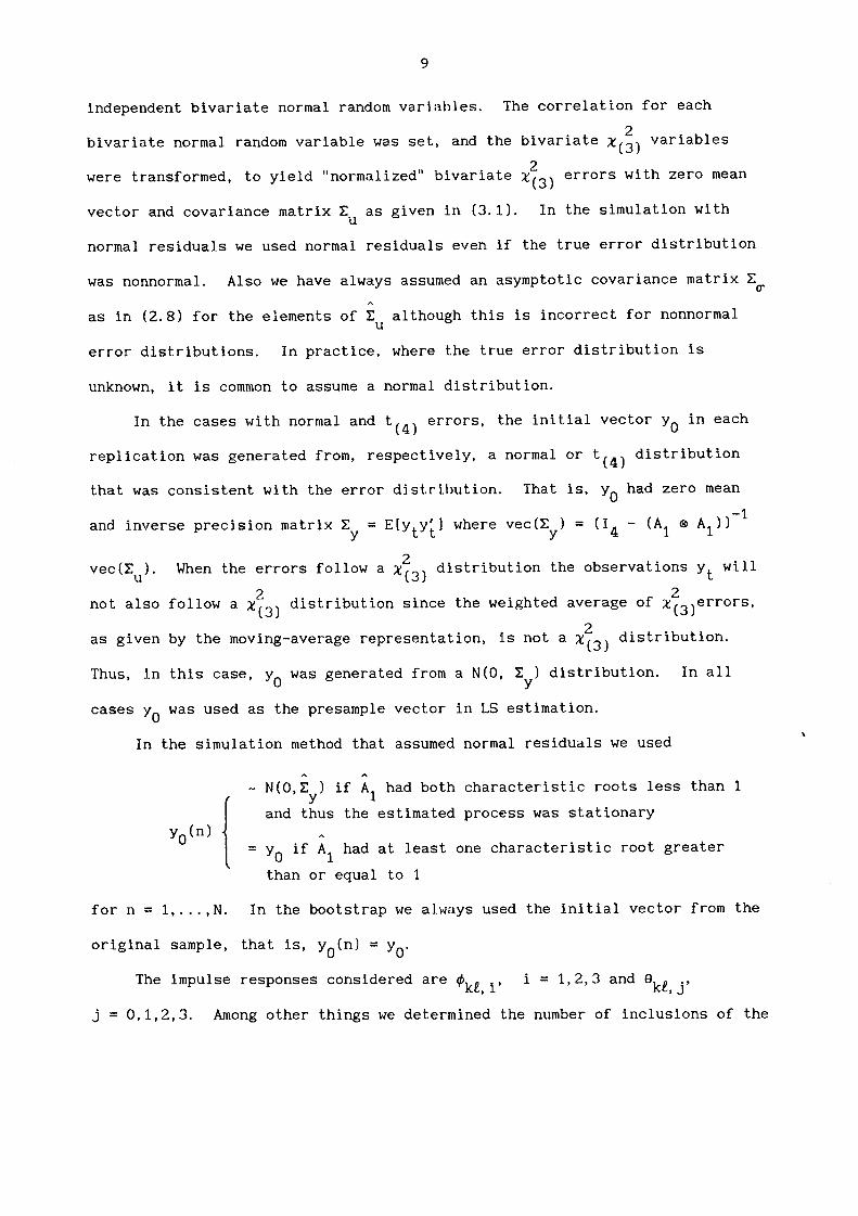
independent bivariate normal random var|,;~b]es. The correlation for each

2bivariate normal random variable was set, and the bivariate X(3) variables

2were transformed, to yield "normalized" bivariate ~(3) errors with zero mean

vector and covariance matrix Z as given in (3.1).U

In the simulation with

normal residuals we used normal residuals even if the true error distribution

was nonnormal. Also we have always assumed an asymptotic covariance matrix

as in (2.8) for the elements of Z although this is incorrect for nonnormalu

error distributions. In practice, where the true error distribution is

unknown, it is common to assume a normal distribution.

In the cases with normal and t(4) errors, the initial vector YO in each

replication was generated from, respectively, a normal or t(4) distribution

that was consistent with the error d~str[bution. That is, YO had zero mean

and inverse precision matrix Zy = E[yty[] where veC(Zy) = (I4 - (A1 ® AI))-I

vec(Zu) When the errors follow a X2¯(3) distribution the observations Yt will

2 2not also follow a X(3) distribution since the weighted average of ~(3)errors,

2as given by the moving-average representation, is not a ~(3) distribution.

Thus, in this case YO was generated from a N(O, Z ) distribution.y

cases YO was used as the presample vector in LS estimation.

In all

In the simulation method that assumed normal residuals we used

YO(n)

^

N(O,Zy) if A1 had both characteristic roots less than 1

and thus the estimated process was stationary^

= YO if A1 had at least one characteristic root greater

than or equal to 1

for n = 1 ..... N. In the bootstrap we always used the initial vector from the

original sample, that is, YO(n) = YO"

The impulse responses considered are Ck~,i’ i = 1,2,3 and eke, j,

j = 0,1,2,3. Among other things we determined the number of inclusions of the

I0

true impulse response coefficients in 90% and 95% confidence intervals

estimated by the 5 methods listed in the previous section.

Two sample sizes were considered, T = 50 and T = I00. The results for

T = 50 are based on a different set of random numbers than those for T = I00.

In each replication the number of boots|.r’ap and simulation runs is N = i00.

Since preliminary experiments with N = 200 did not lead to much change in the

results, the smaller N was settled upon. The number of replications for

each set of parameter values is R = 200. Finally, the programs used to

perform the computations were written in SHAZAM.

4. The Results

Qualitatively similar results were obtained for 90% and 95% confidence

intervals. Therefore we will concentrate on 95% intervals as they seem to be

the more common ones used in practice. We will discuss the dependence of

the results on the parameter values, the error distribution and the sample

size.

We will begin with a discussion of the results for the � impulse

responses. For these we have set ¢12 = 0.3. Preliminary simulations with

other Z matrices did not yield results that prompted further investigation.u

A small correlation coefficient was felt to be a common occurrence in applied

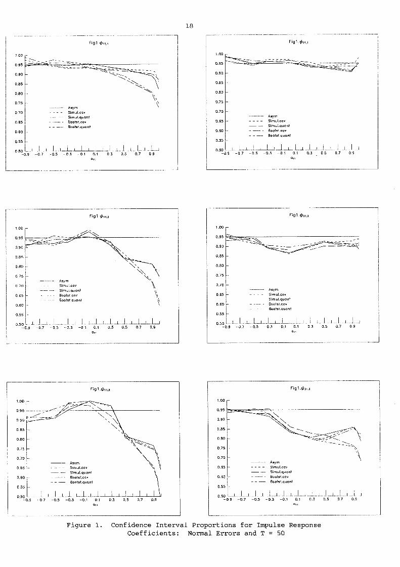
work with real data. In Figure I the proportions of inclusions of $ll,i and

in estimated 95% confidence intervals are plotted for normal errors,¢21,isample size T = 50, a21 = a22 = 0.5, and different values of all. A

nonstationary, cointegrated process is included as a boundary case for

all = I. The asymptotic variances of all impulse response coefficients are

nonzero so that the standard asymptotic theory remains valid. From the figure

it can be seen that for lag 1 (where ¢11,1 = all and ¢21,1 = a21) all methods

perform about equally well. An exception is the confidence intervals for

II

¢II, i for values of all that approach I; under these circumstances the two

empirical quantile methods are considerably worse than the other methods and

fall well below what could be attributed to sampling variability. In a Monte

Carlo experiment with 200 replications the standard error for the proportion

estimates is 0.015, so, roughly speaking, proportion estimates that llew

between 0.92 and 0.98 can be considered reasonable (or attributable to sample

variability). For higher lags the actual confidence level differs even more

from the intended theoretical level of 95Z, and for all methods and for a

larger part of the parameter space. It is interesting to note that the

direction of the deviation from the intended level is the same for all methods

and there is no clearly superior or clearly inferior method over the whole

parameter space, although for the cointegrated process, and for large positive

all, the quantile methods 3 and 5 perform markedly poorer than the other

methods.

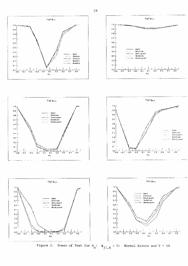
In Figure 2 we have depicted the proportions of inclusions of zero in

estimated confidence intervals for ~ll, i and ~21, i" Often one will be

interested in whether there is an effect at all from an impulse in one

variable. As a crude test one might check whether zero falls within the

confidence intervals for the response coefficients. Thus, in Figure 2 the

power of such a test for an individual coefficient is depicted. For lag I the

power of all methods is quite similar. For lag 2 a slight superiority of the

quantile methods becomes visible for all values close to zero. For lag 3 this

superiority is quite strong, and extends to negative values of all when

testing ~II,3"

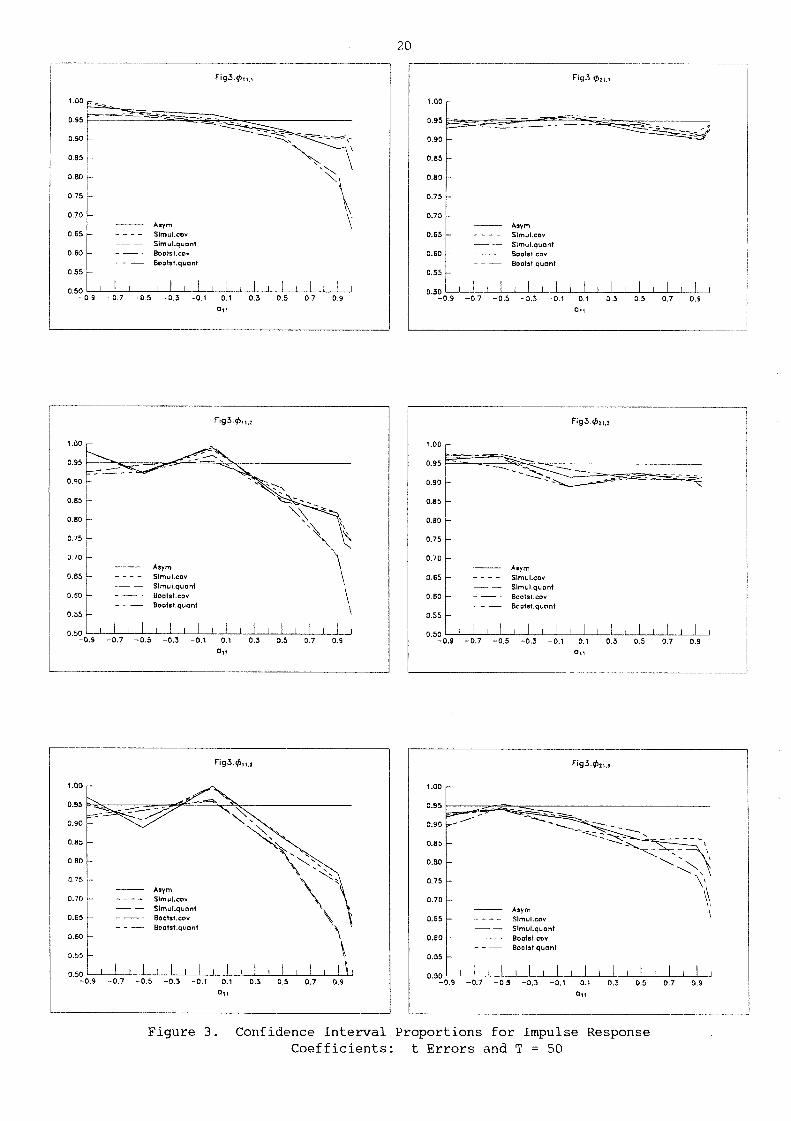
Figure 3 corresponds exactly to Figure 1 except that the error

distribution of the underlying processes is a bivariate t rather than a

normal. For nonnormal errors one might expect an advantage from bootstrapping

12

methods, while the simulation methods a~’e actually performed on false

assumptions. This, however, is not reflected in the results which are largely

similar to those from the normal error case. The same turned out to be true

2for the ~(3) errors. We will therefore not report the results here.

Increasing the sample size from T = 50 to T = I00 did not cllhange the

situation drastically. In particular the general patterns in Figures 1 - 3

did not change much although the estimated confidence levels were overall

closer to the intended level of 95Z and the powers increased where they had

not been i before. It is interesting, however, that the relative power

advantage of the quantile methods 3 and 5 for values of all close to zero was

maintained. To conserve space we do not give the results in detail here.

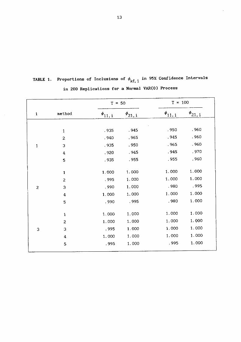
We have also considered processes wl.th A1 = 0 for which some asymptotic

variances are zero. Of course, these processes are actually VAR(0) or white

noise processes. In practice this information is often not available and we

fitted VAR(1) processes to the generated data. In this situation it can be^

shown that the asymptotic variances of Okg, i are zero for i = 2,3 .... Thus,

for these impulse responses the standard asymptotic approach may give

misleading results because the estimators converge to the true values of zero

more rapidly than at the usual 4-~--rate. In Table 1 we give some estimated

confidence levels based on normal residuals. They clearly show that for lags

2 and 3 the intended level of 95Z understates the nominal level markedly.

Surprisingly, however, the simulation and bootstrapping methods are biased in

the same direction as the asymptotic theol’y. In other words, they also

provide confidence intervals with more than 95Z probability content. The

situation does not improve significantly for T = i00.

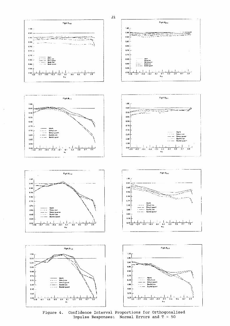
Let us now turn to the results for orthogonalised impulse responses. In

Figure 4 the proportions of inclusions of 811,i and 821,i in estimated 95Z

13

TABLE 1. Proportions of Inclusions of Ck~,i in 95% Confidence Intervals

in 200 Replications for a Normal VAR(0) Process

T = 50 T = I00

method �ii,i ¢21,i �11, i ¢21, i

2

3

1 .935 .945 .950 .960

2 .940 .965 .945 .960

3 .935 .950 .965 .960

4 .920 .945 .945 .970

5 .935 .955 .955 .960

1 1.000 1.000 1.000 1.000

2 .995 1.000 1.000 1.000

3 .990 1.000 .980 .995

4 1.000 1.000 1.000 1.000

5 .990 .995 .980 1.000

I

2

3

4

5

1.000 1.000 1.000 1.000

1.000 1.000 1.000 1.000

.995 1,000 1.000 1.000

1.000 1.000 1.000 1.000

.995 1.000 .995 1.000

i4

confidence intervals are displayed for Gaussian (normal) VAR(1) processes with

~13 = 0.3, a12 = a22 = 0.5, varying all values and sample size T = 50. Thus,

Figure 4 corresponds to Figure 1 which relates to the ¢ impulse responses.

The overall conclusions emerging from Figure 4 are similar to those from

Figure I. Specifically, all methods tend to be biased in the same direction.

That is, the proportions of inclusions of the true parameter value in 95Z

confidence intervals tend to be lower than 95Z for all the methods or they

tend to be larger than 95Z for all the methods, depending on the value of all

and the lag i of the impulse responses. None of the methods is superior over

the whole range of all values, and the quantile methods tends to be inferior

for large positive values of all and the cointegrated case.

Although we do not give the results here in detail in order to conserve

space, we note that the quantile methods 3 and 5 had power advantages for

higher lags (i = 2,3) and small values of all, as for the ~ impulse responses.

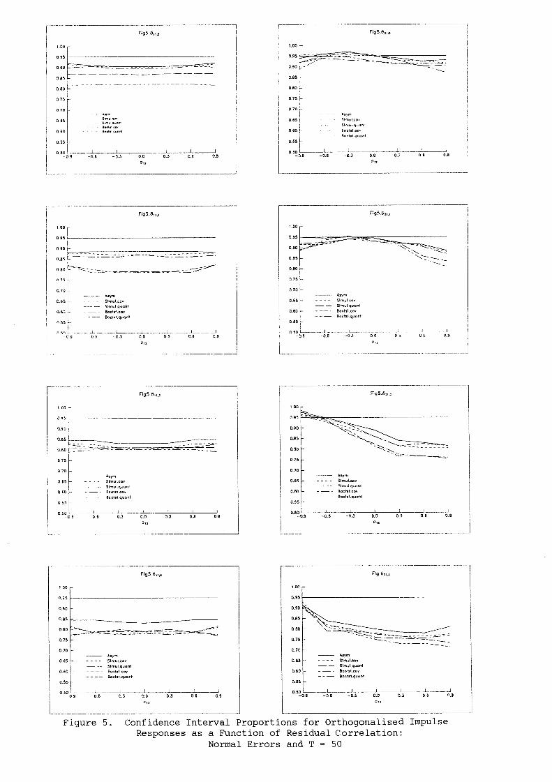
In Figure 5 similar results for varying values of the residual

correlation ff12 are given for T = 50 and all = a21 = a22 = 0.5. Again

asimilar picture emerges as in Figure 4. With the exceptions of 821,2

the results are fairly insensitive to the residual correlation.821,3

the five methods does particularly well in matching the true and intended

confidence intervals of 95Z when there is a high positive residual

correlation.

and

None of

In some cases the quantile methods are markedly inferior to the

other methods.

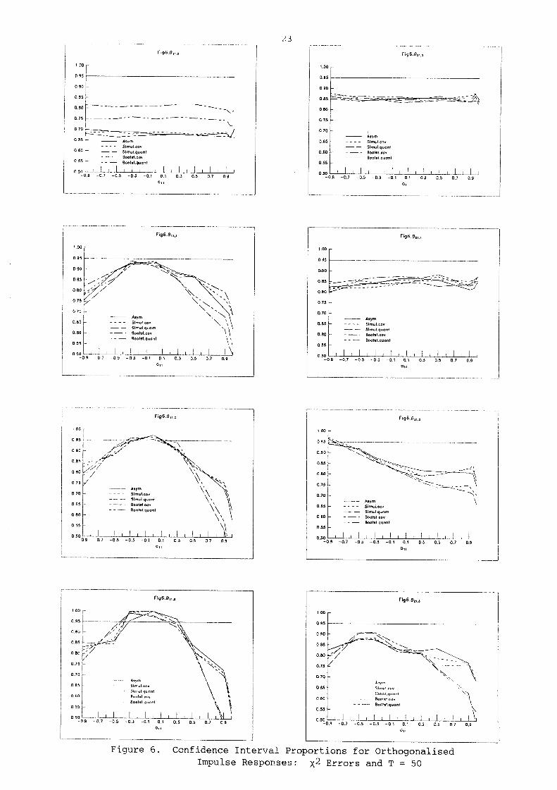
As pointed out in Section 3, the asymptotic distribution of the 8 impulse

responses depends critically on the true distribution of the process.

Therefore one would expect the quantile bootstrap method 5 to be superior for

nonnormal error distributions since it is the only one that does not

incorporate any assumption regarding the process distribution. Some results

2 errors are depicted in Figure 6. Surprisingly the bootstrap methodsfor ~(3)

are not generally superior to the asymptotic theory and the simulation methods

that are based on normal residuals. The performance of all the methods is not

satisfactory for this case and they are all biased in the same direction.

5. Conclusions

Since the Monte Carlo setup is necessarily limited some caution is

required in drawing general conclusions from the results. There are, however,

some observations that we can make. It is obvious that none of the methods is

generally superior in terms of confidence level and power. Since all

simulation methods are relatively expenslve in terms of computer time it may

be advisable to use the computationally efficient confidence bounds obtained

on the basis of asymptotic theory, at least as a first check. In our

Monte Carlo investigation their size was biased in the same direction as

that of the other methods. In other words, when the asymptotic confidence

intervals had a higher or lower level than the intended one the other methods

had the same tendency. The power of the asymptotic methods may be lower,

though, at higher lags and for small parameter values than that of the

quantile methods. In other words, if the asymptotic confidence bounds

indicate significant responses to an impulse in one variable, we can be

reasonably sure that something is really going on in the system. If no

significant impulse responses are found In this way a check with the quantile

simulation methods may be advisable.

The poor performance of all methods for some parameter values is a

concern especially as it does not go away quickly when the sample size

increases. This lends support to those who doubt that precise quantitative

16

statements regarding the impulse responses can be made if unrestricted VAR

models are being fitted.

Further research is required to confirm whether the foregoing results are

of general validity in practical application of the VAR methodology. In

particular it would be of interest to see whether the results depend on the

dimension and order of the process. Also, in practice, the order of the data

generation process is normally unknown. Therefore it is usually chosen

according to some method or criterion. The impact of such strategies on the

properties of the estimated impulse responses would also be of interest.

Furthermore, investigating the effect of imposing parameter constraints either

exact or of a Bayesian variety would be desirable. All these issues are left

for future research.

17

References

L~tkepohl, H. (1988), "Asymptotic Distribution of the Moving Average

Coefficients of an Estimated Vector Autoregressive Process", Econometric

Theory, 4, 77-85.

L~tkepohl, H. (1990), "Asymptotic Distributions of Impulse Response Functions

and Forecast Error Variance Decompositions of Vector Autoregresslve

Models", Review of Economics and S[~li:i.stics, forthcoming.

Magnus, J.R. and H. Neudecker (i988), Matrix Differential Calculus with

Applications in Statistics and Econometrics, Chichester: John Wiley.

Park, J.Y. and P.C.B. Phillips (1989), "Statistical Inference in Regressions

with Integrated Processes: Part 2", Econometric Theory, 5, 95-131.

Sims, C.A. (1980), "Macroeconomics and Reality", Econometrica, 48, i-48.

&95

3.80

0,70 Simul.cov

0.60

0.55 ~

18

Fig1 ,li6~tJ

t

0.90 10.85 l

o.8o ~-

0.75

0.70 FAsym

0.65 .... Slmul.¢ovSlmuLquant

Boo|st.qu(Int0.55 ~

Fig1 45zi.2

51mul.covSlmul.quonfBoutst.covBootst.quan!

0 85

0.80

0.70 Asym

- 0.9 - 0.7 --0,5 -0,3 -0,1 O.t 03 0.5 0,7 0,9

Figl-~zLs

"I .00

0.95

0.90

D.85

0.80

0.75

0.70

0.65

0.50

0.55

ARmSlmul.covSlmul.quont

Bootst.qucint

-0.9 -0.7 -0,5 -0,3 -0,1 0.1 0,3 0,5 0,7 0,9

Figure i. Confidence Interval Proportions for Impulse ResponseCoefficients: Normal Errors and T = 50

o o __±__LL~_.~_.L_.L__Lll I i I I I I I I I I

19

0.9 !

0.8

0.7

0.6

0.2

0.!

Fig2.~H.t Fig2 q%:mz

0.9 -0.7 -0.5 -0,3 -0,1 O.t 0,3 0.5 0.7

Figure 2. Power of Test for H :o

2O

0.85

0.80

0.75

0.70

0.55

1

0.90 I

0.85

0.80

o.7s 1

0.70

0.65 SlmuLcovSimul.quont

0.60 I Bootst,cov- - -- Bootst.quant

0.ss ~

-0.9 -0.7 -0.5 -0.3 -0. I 0.1 0.3 0.5 0.7 0.9

AsymSlmul,cov \

0.55

Fig 3.~)z,.z

1.00 ~

0.95 !

0.90 ~

0.85 L

0.60 F

0.70 tAsym

0.55 ~" Slmul.cov

0.60 lSlmul.quontBool~t,cov

0.55 t - - -- Bootst.quont

Fig3.¢,j

-0,9 -0.7 -0,5 -0,3 -0,1 0.1 0,5 0,5 0,7 0,9

Fig3.¢zt.~

1.00 I--

0.95 !

0.85 ~\

0.80

0.75

0.70

Asym \O+6~ I SlmuLcov

$1muLquant0.60

Bootst.quan|0,55 --

Figure 3. Confidence Interval Proportions for Impulse ResponseCoefficients: t Errors and T = 50

2t

-0~ -0.7 -0.5 -0.3 -0.I 0.1 0.3 0.5 0 7 0.9

Figure 4. Confidence Interval Proportions for OrthogonalisedImpulse Responses: Normal Errors and T = 50

’°°I

.... S~mul.quant

Figure 5. Confidence Interval Proportions for Orthogonalised ImpulseResponses as a Function of Residual Correlation:

Normal Errors and T = 50

23

o~oI

Figure 6. Confidence Interval Proportions for OrthogonalisedImpulse Responses: X2 Errors and T = 50

WORKING PAPERS IN ECONOMETRICS AND APPLIED STATISTICS

The Prior Likelihood and Best Linear Unbiased Prediction in StochasticCoefficient Linear Models. Lung-Fei Lee and William E. Griffiths,No. 1 - March 1979.

Stability Cbnditions in the Use of Fixed Requirement Approach to ManpowerPlanning Mod~ls. lloward E. Doran and Rozany R. Deen, No. 2 - March1979.

A Note on A Bayesian Estimator in an Autocorrelated Error Model.William Griffiths and Dan Dao, No. 3 - April 1979.

On R2-Statistics for the General Linear Model w~th Nonsoalar Covar~[anaeMatrix. G.E. Battese and W.E. Griffiths, No. 4 - April 1979.

Const~ation of Cost-Of-LiuzU~g Index Numbers - A Un{~f~Zed Approaoh.D.S. Prasada Rao, No. 5 - April 1979.

Omission of the Weighted First Observation in an Autocorrelated RegressionModel: A Discussion of Loss of Efficiency. Howard E. Doran, No. 6 -June 1979.

Estimation of Household Expenditure Functions: An Application of a Classof Heteroscedastic Regression Models. George E. Battese andBruce P. Bonyhady, No. 7 - September 1979.

The Demand for S~an Timber: An Application of the Piewert Cost Function.Howard E. Doran and David F. Williams, No. 8 - September 1979.

A New System of Log-Change Index Numbers for Multilateral Comparisons.D.S. Prasada Rao, No. 9 - October 1980.

A Comparison of Purchasing Power Parity Between the Pound Sterling andthe Australian Dollar - 1979. W.F. Shepherd and D.S. Prasada Rao,No. i0 - October 1980.

Using Time-Series and Cross-Section Data to Estimate a Production Functionwith Positive and Negative Marginal Risks. W.E. Griffiths andJ.R. Anderson, No. ii - December 1980.

A Lack-Of-Fit Test in the Presence of Heteroscedasticity. Howard E. Doranand Jan Kmenta, No. 12 - April 1981.

On the Relative Efficiency of Estimators Which Include the InitialObservations in the Estimation of Seemingly Unrelated Regressionswith First Order Autoregressive Disturbances. H.E. Doran andW.E. Griffiths, No. 13 - June 1981.

An Analysis of the Linkages Between the Consumer Price Index and theAverage Minimum Weekly Wage Rate. Pauline Beesley, No. 14 - July 1981.

An Error Components Model for Prediction of County Crop Areas Using Surveyand Satellite Data. George E. Battese and Wayne A. Fuller, No. 15 -February 1982.

N~!.working or Transhipment? Optimisation AlternatT~ds ~or rZcvz{: l,c~’~z{,~’,~Dea[,~i.ons. 11.I. Tort and P.A. Cassidy, No. 16 - February 1985.

Modcll~. II.E. l)o~an, No. 17 - February ]985.

A Purther Considenation of Causal Relationships B~tween Wage:, and

J.W.B. Guise and P.A.A. Beesley, No. ~8 - February 1985.

W.E. Griffiths and K. Surekha, No. 19 - August 1985.

A Walras{an Exchange Equilibrium Interpretation of the Geary-Kh~nis]n~e~v~at~ona~ Pr{ce8. D.S. Prasada Rao, No. 20 - October .1985.

~’:n Us~[ng {)unbin’s h-Test to Valid~te the Partia~-Adjustme,~t Mode~..H.E. Doran, No. 21 - November 1985.

A~ {nv(:st~gation b~to the ~gnaZ l Sample Propert ~es of Cou~u,iance Mat~,ixand Pre-Test Estimatons for the P~obit Mode{.. William ~. Gr~ffiths,R. Carter Hi_ll and Peter J. Pope, No. 22 - November 1985.

At~s~ra~[an Z)(z[~p~.l ]~dz~sZ, p~.4. T.J. Coelli and G.E. Batt:(,so., No. 24 -February |98¢~.

l,eu~./ t’nod~,t:~:on Function,s Using Agg~,egat~im:~. l)al.a. George E. Batteseand Sohail d. Malik, No. 25 - April 1986.

Estimation of Etast~cit(es of Substitution for CES P~’oduatiwn FunctionsUsing Aggregative Data on Selected Manufacturing Industnies in Pakistan.George E. Battese and Sohail J. Malik, No.26 - April 1986.

Estimation of Elasticities of Substitution ]br CES and VES P~’oductionFunctions Using Fi~n-Leuel Data for Food-Processing _bzdustries inPakistan. George E. Battese and Sohail J. Malik, No.27 - May 1986.

On the Prediot~’~on of Techni(;al Effioienaies, <;h)en the Sp{’.<;ifioat:ion.~ of aGeneratized Fnontie~, P~’oduction Function and lhnel Data ok~ {;ample l;’i~,ma.George E. Battese, No.28 - June 1986.

A General Equi~ib~,iz~m App~,oach to the Const~otion of MuLt~/at~’aZ IndexNumbers. D.S. Prasada Rao and J. Sa]azar-Carri]lo, No.29 - August1986.

Further Results on J-nte~,uaT~ E:~timation in an AR(1) Em,o~, Mode7.W.E. Griffiths and P.A. Beesley, No.30 -August 1987.

Bayesian Eoonometnics and How to Get Rid of Tho~e ~’ong Signs.Griffiths, No.31 - November 1987.

H.E. Doran,

William E.

3o

Confidence Inte~,uals for the Expected Auerage Marginal Prod~cl;s ofCobb-Douglas Faotons With Applioat~ons of A’~tz~mat~n~ S;z~dow F~,z’~.~esand Testing for Rf~k Auensf, on. Chris M. Aka~uz, e, N~. 3,t -Septe~er, 1988.

Estimation of Frontier Production Functions and the Effiaiencies ofIndian Far~s Using Panel Data from ICRI$AT’s Village Level Studies.G.E. Battese, T.J. Coelli and T.C. Colby, No. 33 - January, 1989.

Estimation of Frontlet~ Production Functions: A Guide to the ComputerProgram, FRONTIER. ’fire J. Coelli, No. 34 - February, 1989.

An Introduction to Austral[,a~ Economy-Wtde ModeZ{,ing. colin p. Hargreaves,No. 35 - February, i[989.

Testing and E~timating l,owation Vectors Under llet~roske~bt~rtiw~ty.William Griffiths and George Judge, No. 36 - February, 1989.

The Management of lrrigat[~on Water During Drwught. Chris M. Alaouze,

No. 37 - April, 1989.

inverse of the Distribution Function of a Strictly Fosit~[ve RandomVariable with Applications to Water Allocation Problems.Chris M. Alaouze, No. 38 - July, 1989.

A Mixed Integer Linear Progra.~ning Eualuation of Salinity and WaterloggingControl Options in the Murray-Darling Basin of Australia.Chris M. Alaouze and Campbell R. Fitzpatrick, No. 39 - August, 1989.

Estimation o~" Risk Effects with Seemingly Unrelated Regressions andPanel Data. Guang H. Wan, William E. Griffiths and Jock R. Anderson,No. 40- September, 1989.

The Optimality of Capactty Sharing in Stochastic Dyn~,ic Progr~nmingProblems of Shared Reservoir Operation. Chris M. Alaouze, No. 41 -November, 1989.

Confidence Internals for impulse Responses f~,om VAR Mode{~:~: A Comparisonof Asymptotic ’l’heo~’y and Simulation Approaches. william G,:iffiths andHelmut L~tkepohl, No. 42 - March 1990.